A Distinguished Vacuum State for a Quantum Field in a Curved Spacetime: Formalism, Features, and Cosmology

Abstract

We define a distinguished “ground state” or “vacuum” for a free scalar quantum field in a globally hyperbolic region of an arbitrarily curved spacetime. Our prescription is motivated by the recent construction Johnston ; RDS of a quantum field theory on a background causal set using only knowledge of the retarded Green’s function. We generalize that construction to continuum spacetimes and find that it yields a distinguished vacuum or ground state for a non-interacting, massive or massless scalar field. This state is defined for all compact regions and for many noncompact ones. In a static spacetime we find that our vacuum coincides with the usual ground state. We determine it also for a radiation-filled, spatially homogeneous and isotropic cosmos, and show that the super-horizon correlations are approximately the same as those of a thermal state. Finally, we illustrate the inherent non-locality of our prescription with the example of a spacetime which sandwiches a region with curvature in-between flat initial and final regions.

1 Introduction

The framework known as “quantum field theory in curved spacetime” concerns the interaction of quantum fields with gravity, but only in an asymmetrical sense. Non-gravitational, “matter” fields are treated in accord with quantum principles while their gravitational “back reaction” is either ignored entirely or described by a semiclassical form of the Einstein equations. Although not a fundamental theory of nature, this framework has provided us with profound insights into an eventual theory of quantum gravity. Important examples include Hawking radiation by black holes Hawking , the Unruh effect bisognano ; Unruh , and the generation of Gaussian-distributed random perturbations in the theory of cosmic inflation Mukhanov . In all these examples a choice of vacuum — or at least a reasonable reference state of the field — is of crucial importance. It therefore seems unsatisfactory that as it stands, quantum field theory lacks a general notion of “vacuum” which extends very far beyond flat spacetime.

Formulations of quantum field theory in Minkowski spacetime do provide a distinguished vacuum, but it rests heavily on a particle interpretation of the field that is closely tied to the properties of the Fourier transform and the availability of plane waves. More abstract treatments tend to trace the uniqueness of the vacuum to Poincare-invariance, but that is tied even more closely to flat space. It is thus unclear how one might extend the notion of vacuum beyond the case of spacetimes with a high degree of symmetry. (Moreover, even a large symmetry-group does not always yield a unique vacuum without further input. In de-Sitter for example, one has the one complex-parameter family of “$\alpha$-vacua” Allen , all of which are invariant under the full de-Sitter group. To single one value of $\alpha$ out from the rest, one needs to impose the further condition that the two-point function take the so-called Hadamard form.)

One might even question whether a quantum field theory is well-defined at all before a vacuum is specified. What is probably the best studied mathematical framework for quantum field theory in flat space, that of the Wightman axioms, incorporates assertions about the vacuum among its basic assumptions, and it relies on them in proving such central results as the PCT and spin-statistics theorems. It is therefore noteworthy that the so-called algebraic approach to quantum field theory has been able to proceed a great distance without relying on a notion of vacuum, or indeed any unique representation of the quantum fields at all. In place of a Poincaré-invariant vacuum, it has been proposed to rely on a distinguished class of states, the so-called Hadamard states (which are well-suited to renormalization of the stress-tensor by “point-splitting”), supplemented by an assumption about a short-distance asymptotic expansion for products of quantum fields, namely the operator product expansion or “OPE” (see for example Wald , Wald2 and references therein). If such a “purely algebraic” approach were to establish itself more generally, it might diminish the interest in distinguished “vacua” for curved spacetimes. Conversely, if a reasonable definition of a preferred vacuum state could be obtained it might remove some of the motivation for a purely algebraic formulation of quantum field theory.

Let us remark also that histories-based formulations of quantum mechanics tend to fuse the concept of state with that of equation of motion. This shows up clearly in formulations that start from the “quantum measure” DJS ; RDS2 ; RDS3 or “decoherence functional” Hartle , neither of which can be defined without furnishing a suitable set of “initial conditions”. In this sense, one has no dynamical law at all before a distinguished “initial state” is specified.

At a less formal level, the ability to think in terms of particles offers an obvious benefit to one’s intuition. And, especially in relation to cosmology, great interest attaches to the question whether certain sorts of states can be regarded as “natural” to certain regions of spacetime, a question we return to briefly in section 5.2. These, then, are two more reasons why the availability of a distinguished vacuum could be welcome, whether or not it is logically necessary to quantum field theory as such.

Moreover, what is logically necessary can change drastically if one passes from the spacetime continuum to some more fundamental structure, especially if that structure is discrete. As we will review later, the entire quantization process — as usually conceived — boils down to selecting an appropriate subspace of the solution space of the Klein-Gordon equation. But that way of organizing the problem seems to break down in the case of a causal set. There, the notion of “approximate solution” seems to be the best that is available, and one therefore requires a different starting point.

In Johnston , such a starting point was found in (the discrete analog of) the retarded Green function. On that basis a complete counterpart of the quantum field theory of a free scalar field was built up, and a unique “vacuum state” was derived. Herein, we generalize that derivation to quantum fields on continuum spacetimes, showing thereby that there is a sensible way to uniquely define a vacuum state for a scalar field in any globally hyperbolic spacetime or region of spacetime. More precisely, we consider the case of a free scalar field in a globally hyperbolic spacetime or region of spacetime, and in that context we put forward a definition of distinguished vacuum state that applies to all compact regions and to a large class of noncompact regions.

It is thus possible to carry the concept of vacuum far beyond the confines of Minkowski space by means of definitions we expose in detail below. Although, for all of the reasons indicated above, this possibility is of interest in itself, one naturally wants to know to what extent, and in what sense, our proposal is “the right one”? To that question, only a sufficient number of particular instances of our vacuum would seem to be germane. The examples of Minkowski spacetime and of globally static spacetimes furnish important evidence, but they contain little that is new physically. To judge the ultimate fruitfulness of our prescription, one should, for example, test it against the behavior of the “matter fields” that one actually encounters in the early universe. In Section 5 we make a start on this kind of test, beginning with the case of a spatially homegeneous and isotropic cosmology.

2 Background

In this section, we briefly review the quantization, along traditional lines, of a free scalar field on a curved spacetime. We will be a bit careful with the mathematical technicalities because it will benefit us later. Consider a free, real-valued scalar field $\phi$ on a globally hyperbolic spacetime ($M$, $g_{\mu\nu}$) satisfying the Klein-Gordon equation with mass-parameter $m\geq 0$:

$$\nabla^{\mu}\nabla_{\mu}\phi(x)+m^{2}\phi(x)=0\ ,$$ (1)

where $\nabla_{\mu}$ is the covariant derivative operator on $M$.  The condition of global hyperbolicity ensures that (1) has a well posed initial-value formulation (see theorem 29 in Appendix B).

Let us review some mathematical structures that are important for both the classical and quantal theories of a free field. Consider a foliation of $M$ by spacelike Cauchy surfaces $\Sigma_{t}$, labeled by a time parameter $t$. Let S be the space of all real $\textrm{C}^{\infty}$ solutions of (1) which induce initial data of compact support on some (and therefore on every) $\Sigma_{t}$. (This restriction on the solutions is just for convenience, so that various mathematical structures are well-defined.) The retarded and advanced Green’s functions $G_{R,A}(x,y)$ associated with (1) satisfy

$$(\nabla^{\mu}\nabla_{\mu}+m^{2})G_{R,A}(x,y)=-\frac{\delta^{4}(x-y)}{\sqrt{-g}},$$ (2)

where $g$ is the determinant of the metric-tensor. By definition $G_{R}(x,y)=0$ unless $x\succ{y}$ (meaning $x$ is inside or on the future lightcone of $y$), and $G_{A}(x,y)=0$ unless $x\prec y$.

The so-called Pauli-Jordan function is defined as

$$\Delta(x,y)\equiv G_{R}(x,y)-G_{A}(x,y)=G_{R}(x,y)-G_{R}(y,x)\ .\$$ (3)

From it we define an integral operator $\Delta$:

$$(\Delta f)(x)\equiv\int_{M}\Delta(x,y)f(y)\,\mathrm{d}V_{y},$$ (4)

where $dV_{y}=\sqrt{-g(y)}d^{4}y$ is the metric volume element on $M$, and we take the domain of $\Delta$ to be the space $\textrm{C}_{0}^{\infty}(M)$ of all smooth functions of compact support on $M$. Since $\Delta f$ is the difference between two solutions of the inhomogeneous Klein-Gordon equation with the same source $f$, it satisfies the homogeneous Klein-Gordon equation (1):

$$(\Box+m^{2})\Delta=0\ ,$$ (5)

where $\Box=\nabla_{\mu}\nabla^{\mu}$. Moreover, since $f$ has compact support, $\Delta f$ induces smooth initial data of compact support on all Cauchy surfaces, making $\Delta$ a map from $\textrm{C}_{0}^{\infty}(M)$ to S. The operator $\Delta$ (or more generally the corresponding quadratic form) will be of crucial importance to us. A symplectic structure $\Omega:\textbf{S}\times\textbf{S}\rightarrow\mathbb{R}$ can be defined on S:

$$\Omega(\phi_{1},\phi_{2})\equiv\int_{\Sigma_{t}}\left[\phi_{1}\nabla_{\mu}\phi_{2}-\phi_{2}\nabla_{\mu}\phi_{1}\right]dS^{\mu}\ ,$$ (6)

where $dS_{\mu}=n_{\mu}\sqrt{-h}\,\mathrm{d}^{3}x$ with $n^{a}$ the unit normal to $\Sigma_{t}$, and $h$ the determinant of the induced metric on $\Sigma_{t}$. The righthand side of (6) is well defined because it is independent of $t$ for all solutions in S.

To pass to the quantum theory, one introduces operator-valued distributions $\widehat{\phi}(x)$ that satisfy the Klein-Gordon equation, and the canonical commutation relations (CCR)

$$[\widehat{\phi}(f),\widehat{\phi}(g)]=i\Omega(\Delta f,\Delta g)=i\int_{M}f(x)\Delta(x,y)g(y)\,\mathrm{d}V_{x}\,\mathrm{d}V_{y}\ ,$$ (7)

for all $f,g\in\textrm{C}_{0}^{\infty}(M)$, where $\widehat{\phi}(f)=\int_{M}\widehat{\phi}(x)f(x)dV_{x}$. The second equality follows from theorem 30 (see Appendix B). Equation (7) is typically expressed as

$$[\widehat{\phi}(x),\widehat{\phi}(y)]=i\Delta(x,y).$$ (8)

To obtain operators in Hilbert space, one requires further a $*$-representation of these relations. One typically works with irreducible, Fock representations constructed as follows:

• Complexify the Klein-Gordon solution space to get $\textbf{S}_{\mathbb{C}}=\{\phi_{1}+i\phi_{2}|\phi_{1},\phi_{2}\in\textbf{S}\}$.

• Define a map $(\,,\,)_{KG}:\textbf{S}_{\mathbb{C}}\times\textbf{S}_{\mathbb{C}}\to\mathbb{C}$ by $(\phi_{1},\phi_{2})_{KG}=i\Omega(\overline{\phi}_{1},\phi_{2})$, where the bar denotes complex conjugation. This map enjoys all the properties of a Hermitian inner product except that it’s not positive definite.

• Choose any subspace $\mathcal{H}\subset\textbf{S}_{\mathbb{C}}$ with the following properties:

  • The inner product $(,)_{KG}$ is positive definite on $\mathcal{H}$, thus making $\mathcal{H}$ into a (pre-)Hilbert space over $\mathbb{C}$.

  • $\textbf{S}_{\mathbb{C}}$ is equal to the span of $\mathcal{H}$ and its complex conjugate space $\overline{\mathcal{H}}$.

  • For all $\phi^{+}\in\mathcal{H}$ and $\phi^{-}\in\overline{\mathcal{H}}$, we have $(\phi^{+},\phi^{-})_{KG}=0$.

The Hilbert space is then taken to be the symmetric Fock space associated with $\mathcal{H}$, the field operators being defined as

$$\widehat{\phi}(x)=\sum_{i}\psi_{i}(x)\widehat{a}_{i}+\overline{\psi}_{i}(x)\widehat{a}^{\dagger}_{i},$$ (9)

where $\{\psi_{i}(x)\}$ is any orthonormal basis of (the Cauchy-completed) $\mathcal{H}$ with respect to the inner product $(,)_{KG}$, and where $\{\widehat{a}_{i}\}$ are the annihilation operators associated with $\{\psi_{i}\}$, satisfying the usual commutation relations, $[\widehat{a}_{i},\widehat{a}_{j}]=0$, $[\widehat{a}_{i},\widehat{a}^{\dagger}_{j}]=\delta_{ij}$. To show that (9) satisfies the CCR, write $\widehat{\phi}(f)=\sum_{i}\big{(}\int_{M}\psi_{i}f\big{)}\widehat{a}_{i}+\big{(}\int_{M}\overline{\psi}_{i}f\big{)}\widehat{a}^{\dagger}_{i}=-i\sum_{i}(\overline{\Delta f},\psi_{i})_{KG}\widehat{a}_{i}+(\overline{\Delta f},\overline{\psi}_{i})_{KG}\widehat{a}^{\dagger}_{i}$, where in the last equality we have used Theorem 30. Then

$$[\widehat{\phi}(f),\widehat{\phi}(g)] = -\sum_{i}(\overline{\Delta f},\psi_{i})_{KG}(\overline{\Delta g},\overline{\psi}_{i})_{KG}-(\overline{\Delta f},\overline{\psi}_{i})_{KG}(\overline{\Delta g},\psi_{i})_{KG}$$ (10)

$$= (\overline{\Delta f}|\sum_{i}|\psi_{i})_{KG}(\psi_{i}|-|\overline{\psi}_{i})_{KG}(\overline{\psi}_{i}||\Delta g)$$

$$= (\overline{\Delta f},\Delta g)_{KG}=i\Omega(\Delta f,\Delta g),$$

where we have used the fact that $\sum_{i}|\psi_{i})_{KG}(\psi_{i}|-|\overline{\psi}_{i})_{KG}(\overline{\psi}_{i}|$ is the identity operator on $\textbf{S}_{\mathbb{C}}$ (because $\{\psi_{i}\}$’s satisfy $(\psi_{i},\psi_{j})_{KG}=\delta_{ij}$, $(\psi_{i},\overline{\psi}_{j})_{KG}=0$, and $(\overline{\psi}_{i},\overline{\psi}_{j})_{KG}=-\delta_{ij}$). Finally, the vacuum is defined as the state annihilated by all $\widehat{a}_{i}$: $\widehat{a}_{i}\,|0\!>\,=0$.

The trouble, of course, is that the subspace $\mathcal{H}\subset\textbf{S}_{\mathbb{C}}$ is not unique. Even if we limit ourselves to Fock representations, there are many ways to choose $\mathcal{H}$, and with each one comes a different set of operators $\widehat{a}_{i}$ and a different vacuum.

3 The S-J Vacuum

The kernel $i\Delta(x,y)$ defined by (3) has two basic properties:

• Antisymmetric — because $G_{A}(x,y)=G_{R}(y,x),$

• Hermitian — i.e. $\overline{i\Delta(y,x)}=i\Delta(x,y)$.

Let $L^{2}(M)$ denote the Hilbert space of all square-integrable functions on $M$ with the usual inner product

$$<\phi,\psi>\;=\int_{M}\overline{\phi}(x)\psi(x)\,\mathrm{d}V_{x}\ .$$ (11)

Then, the integral operator $i\Delta$ associated with $i\Delta(x,y)$ [defined in (4)] will be Hermitian on a subspace of $L^{2}(M)$: $<\phi,i\Delta\psi>\,=\,<i\Delta\phi,\psi>$ for all $\phi$ and $\psi$ in the domain of $i\Delta$. Strictly speaking, $i\Delta$ is in general only a densely defined quadratic form in $L^{2}(M)$, but in introducing our prescription of a vacuum, let us at first set aside the functional-analytical subtleties associated with the domain of $i\Delta$ and assume it to be a self-adjoint operator on $L^{2}(M)$, so that $i\Delta(x,y)$ can be “diagonalized” in the sense of the spectral theorem. We can now state our prescription for a distinguished state, which we call the S-J vacuum after the authors of Johnston ; RDS .

Assuming that $i\Delta$ is selfadjoint, a vacuum state $|SJ\!\!>$ can be defined covariantly via $<\!SJ|\;\widehat{\phi}(x)\,\widehat{\phi}(y)\,|SJ\!>\,=Pos(i\Delta(x,y))$, where $Pos(i\Delta(x,y))$ is the positive spectral projection of $i\Delta$ provided by the spectral theorem.

Informally speaking, this just means the following: $(i)$ construct $\Delta(x,y)$ by anti-symmetrizing the retarded Green’s function, which is uniquely determined from the Klein-Gordon equation in any globally hyperbolic spacetime (see theorem 29 in Appendix B), $(ii)$ diagonalize $i\Delta(x,y)$ in the $L^{2}$ norm, $(iii)$ take its ‘positive part’ to be the two-point function. The spectral theorem gives precise mathematical sense to this prescription so long as $i\Delta$ is self-adjoint.

Of course a two-point function is not yet a full characterization of a state, but it becomes so if we take the state to be “gaussian” by appropriately expressing the $n$-point functions in terms of the two-point function (i.e. by means of the Wick rule). It then will follow, given (9) and (12) below, that the Gel’fand-Naimark-Segal (GNS) representation associated with $|SJ\rangle$ will be a Fock representations with $|SJ\rangle$ playing the role of vacuum.

Let us consider first the special case where $i\Delta(x,y)\in L^{2}(M\times M)$, as is the case in a bounded globally hyperbolic region of 1+1 dimensional Minkowski space, for instance. Then $i\Delta$ becomes a so-called Hilbert-Schmidt integral operator and the following version of the spectral theorem applies RS : there exists an orthonormal basis $\{T_{k}\}_{k=1}^{\infty}$ of $L^{2}(M)$ consisting of eigenfunctions of $i\Delta$ which satisfy $i\Delta T_{k}=\lambda_{k}T_{k}$ with $\lambda_{k}\in\mathbb{R}$. Using this theorem and the fact that $\Delta(x,y)$ itself is real, we deduce $i\Delta\overline{T}_{k}=-\lambda_{k}\overline{T}_{k}$, which in turn makes it possible to split $i\Delta(x,y)$ into a positive and a negative part:

$$i\Delta(x,y)=\sum_{k=1}^{\infty}\lambda_{k}\big{\{}T_{k}(x)\overline{T}_{k}(y)-\overline{T}_{k}(x)T_{k}(y)\big{\}}$$

(taking $\lambda_{k}>0$ now). In this case, our prescription can be expressed as

$$W(x,y)\equiv<SJ|\widehat{\phi}(x)\widehat{\phi}(y)|SJ>=\sum_{k=1}^{\infty}\lambda_{k}T_{k}(x)\overline{T}_{k}(y)\ .$$ (12)

This is equivalent to introducing field operators $\widehat{\phi}(x)=\sum_{k}\sqrt{\lambda_{k}}\big{\{}T_{k}(x)\widehat{a}_{k}+\overline{T}_{k}(x)\widehat{a}_{k}^{\dagger}\big{\}}$, because $(i)$ eigenfunctions of $i\Delta$ with $\lambda\not=0$ necessarily satisfy the Klein-Gordon equation and $(ii)$ the commutation relations are trivially satisfied. The S-J vacuum is then the state in Fock space that is annihilated by all $\widehat{a}_{k}$.

Now let us turn to 3+1 dimensions, where $i\Delta$ is no longer Hilbert-Schmidt. Nonetheless, $i\Delta(x,y)$ is still a distribution and, at least within Minkowski space, it defines a self-adjoint operator if $M$ is bounded (see section A.1 of Appendix A). Thanks to the spectral theorem, our prescription then retains a precise mathematical sense, and it is not too far-fetched to assume that this continues to hold for curved spacetimes, because curvature should not change the singularity structure of $i\Delta(x,y)$ too drastically.

Although selfadjointness might seem to be merely a technical issue, it highlights the fact that the S-J vacuum depends on a choice of (globally hyperbolic) spacetime region. Indeed, as we have just seen, our prescription is not guaranteed to be well defined unless one chooses a region that is bounded, both spatially and temporally. Thus arise two questions: To what extent does our prescription depend on boundary condtions, and to what extent does it remain well-defined in unbounded spacetimes?

In answering the first question, one must distinguish between spatial boundaries (also referred to as timelike boundaries) and temporal ones. Spatial boundaries are familiar to us from putting fields in a box, Casimir effect, etc; and they seem unproblematic. When they are present the S-J vacuum will be sensitive to one’s choice of boundary conditions, because the retarded and advanced Green functions be depend on them. But this is as it should be since the physics genuinely depends on the boundary conditions. We will also consider below regions which are unbounded spatially, but no special difficulties will arise from that feature.

The case of a temporal boundary (spacelike or null) is less familiar. The first thing to notice is that boundary conditions are neither needed nor possible in this case, since the region is (by assumption) globally hyperbolic. Mathematically, this very satisfactory feature stems from the fact that $\Delta$ is not a differential operator but an integral one. Nevertheless, one must bear in mind that the “ground state” one ends up with, does depend on the region with which one begins. In itself, this dependence on the region merely expresses the nonlocal character of our definition. One might for example be interested in which “vacuum” would be appropriate to an early stage of expansion of the cosmos, and one would not want in that case to apply our definition to the full spacetime, including its whole future development. However, one might also want to apply the definition to unbounded spacetimes like Minkowski space, and in such cases one needs to worry about dependence on an eventual infrared cutoff. If the metric is static, for instance, why should time play any role in what the vacuum state looks like?

In dealing with such instances, it is always possible to work first in a truncated spacetime, and later send the temporal boundary to infinity. In section A.2 of Appendix A, we apply this method to the simple harmonic oscillator and show that it succeeds in the sense that the resulting S-J vacuum is the minimum energy state of the Hamiltonian. As we will later demonstrate, this continues to be true for all static spacetimes. Another example of such a calculation can be found in Yasaman , where the spectrum of $i\Delta$ is computed in a 1+1 dimensional causal-diamond, and it is found that (up to the usual infrared ambiguities that affect massless scalars in 2d) the resulting two-point function has the correct (i.e. Minkowski) limiting behaviour as the boundaries of the diamond tend to infinity. However, there are also cases where taking a temporal cutoff to infinity is an ill-defined procedure. In deSitter , it is shown that the so-called Poincaré patch of de Sitter space provides an example of such a case. (We suspect that this kind of ambiguity can be understood intuitively as the failure of $i\Delta$ to admit a selfadjoint extension which is unique. However we don’t know how to pose such a question properly, because $\Delta$ is densely defined only as a quadratic form on $L^{2}(M)$, not as an operator from $L^{2}(M)$ to itself.)

Diagonalizing $i\Delta$ lies at the heart of our prescription, at least in practice. In this section, we will attempt to frame this problem as generally as possible. In subsequent sections, we will deal with more concrete examples. Let $\{u_{k}(x)\}$ be a basis for the Klein-Gordon solution space. Expanding the field operator in terms of these modes as $\widehat{\phi}(x)=\sum_{k}u_{k}(x)\widehat{a}_{k}+\overline{u}_{k}(x)\widehat{a}_{k}^{\dagger}$ and computing the commutator yields, as we have seen,

$$[\widehat{\phi}(x),\widehat{\phi}(y)]=\sum_{k}u_{k}(x)\overline{u}_{k}(y)-u_{k}(y)\overline{u}_{k}(x).$$ (13)

It then follows from the CCR (8) that the integral-kernel $i\Delta(x,x^{\prime})$ takes the form,

$$i\Delta(x,y)=\sum_{k}u_{k}(x)\overline{u}_{k}(y)-\overline{u}_{k}(x)u_{k}(y).$$ (14)

Of course the choice of the $u_{k}(x)$ in this expansion is not unique. Another set of modefunctions $g_{k}(x)=\sum_{n}\alpha_{kn}u_{n}(x)+\beta_{kn}\bar{u}_{n}(x)$ will give the same commutator, so long as the following normalization conditions are met: $\sum_{k}\alpha_{ik}\bar{\alpha}_{jk}-\beta_{ik}\bar{\beta}_{jk}=\delta_{ij}$ and $\sum_{k}\alpha_{ik}\beta_{jk}-\beta_{ik}\alpha_{jk}=0$, this being nothing but a Bogoliubov transformation.

By means of such a transformation, we can find orthonormal eigenfunctions $T_{n}(x)$ of $i\Delta$ (with corresponding eigenvalues $\lambda_{n}$) starting from any convenient basis $\{u_{k}(x)\}$ of the Klein-Gordon solution space. Requiring $T_{n}(x)$’s to be eigenfunctions of $i\Delta$ and using (14):

$$i\Delta\,T_{n}(x)=\lambda_{n}T_{n}(x)=\sum_{k}\langle u_{k},T_{n}\rangle u_{k}(x)-\langle\bar{u}_{k},T_{n}\rangle\bar{u}_{k}(x)\ .$$ (15)

For notational simplicity, let $\alpha_{nk}\equiv\frac{<u_{k},T_{n}>}{\lambda_{n}}$ and $\beta_{nk}\equiv-\frac{<\bar{u}_{k},T_{n}>}{\lambda_{n}}$ so that $T_{n}(x)=\sum_{k}\alpha_{nk}u_{k}(x)+\beta_{nk}\bar{u}_{k}(x)$. These coefficients then satisfy:

$$\alpha_{nk} = \frac{1}{\lambda_{n}}\sum_{m}\alpha_{nm}\langle u_{k},u_{m}\rangle+\beta_{nm}\langle u_{k},\bar{u}_{m}\rangle$$ (16)

$$\beta_{nk} = \frac{-1}{\lambda_{n}}\sum_{m}\alpha_{nm}\langle\bar{u}_{k},u_{m}\rangle+\beta_{nm}\langle\bar{u}_{k},\bar{u}_{m}\rangle.$$ (17)

Requiring these eigenfunctions to be orthonormal ($\forall$ $n,m$) yields

$$\langle T_{n},\bar{T}_{m}\rangle=0 \Longleftrightarrow \sum_{k}\alpha_{nk}\beta_{mk}-\alpha_{mk}\beta_{nk}=0$$ (18)

$$\langle T_{n},T_{m}\rangle=\delta_{nm} \Longleftrightarrow \sum_{k}\bar{\alpha}_{nk}\alpha_{mk}-\bar{\beta}_{nk}\beta_{mk}=\frac{\delta_{nm}}{\lambda_{m}}.$$ (19)

Then, diagonalizing $i\Delta$ boils down to finding $\alpha_{nk}$ and $\beta_{nk}$ by solving these four equations. (We have not addressed the issue of convergence in the sums appearing above. In fact, if it turned out that the $\{T_{n}(x)\}$ and $\{u_{n}(x)\}$ induce unitarily inequivalent representations of CCR, the above sums would not converge.)

It is not obvious how this can be done generically. To proceed, let us simplify this calculation by assuming that there are modefunctions $\{u_{k}(x)\}$ that satisfy

$$\langle u_{k},u_{m}\rangle = \langle u_{k},u_{k}\rangle\delta_{km}$$ (20)

$$\langle u_{k},\bar{u}_{m}\rangle = \langle u_{k},\bar{u}_{-k}\rangle\delta_{k,-m}.$$ (21)

The notation used here is as follows: for every $u_{n}\in\{u_{k}\}$, there is one (and only one) member of the complex conjugate set $\bar{u}_{-n}\in\{\bar{u}_{k}\}$, for which $\langle u_{n},\bar{u}_{-n}\rangle$ can be non-zero. Also, we denote the complex conjugate of $\bar{u}_{-n}$ by $u_{-n}$.

Our assumption is motivated by spacetimes for which these modefunctions are plane waves. Under this assumption, $\alpha_{nk}$ and $\beta_{nk}$ can be found:

$$\alpha_{nk} = \left[\frac{\lambda_{-n}+\langle u_{n},u_{n}\rangle}{\lambda_{n}(\lambda_{n}+\lambda_{-n})}\right]^{\frac{1}{2}}\delta_{nk}$$ (22)

$$\beta_{nk} = -\left[\frac{\langle u_{n},u_{n}\rangle-\lambda_{n}}{\lambda_{n}(\lambda_{n}+\lambda_{-n})}\right]^{\frac{1}{2}}e^{-i\text{Arg}(<u_{n},\bar{u}_{-n}>)}\delta_{n,-k},$$ (23)

where $\lambda_{n}$ is given by

$$2\lambda_{n}=\langle u_{n},u_{n}\rangle-\langle u_{-n},u_{-n}\rangle+\Big{[}\big{(}\langle u_{n},u_{n}\rangle+\langle u_{-n},u_{-n}\rangle\big{)}^{2}-4|\langle u_{n},\bar{u}_{-n}\rangle|^{2}\Big{]}^{\frac{1}{2}}.$$ (24)

By direct substitution, it can be verified that these indeed solve (16), (17), (18) and (19). Finally, the vacuum state modefunctions as picked by our prescription $\mathcal{U}_{n}^{SJ}(x)\equiv\sqrt{\lambda_{n}}T_{n}(x)$ take the form

$$\sqrt{2}\mathcal{U}_{n}^{SJ}(x) = \left[1+\frac{1}{\sqrt{1-\frac{4|<u_{n},\bar{u}_{-n}>|^{2}}{\left(<u_{n},u_{n}>+<u_{-n},u_{-n}>\right)^{2}}}}\right]^{\frac{1}{2}}u_{n}(x)$$ (25)

$$- \left[-1+\frac{1}{\sqrt{1-\frac{4|<u_{n},\bar{u}_{-n}>|^{2}}{\left(<u_{n},u_{n}>+<u_{-n},u_{-n}>\right)^{2}}}}\right]^{\frac{1}{2}}e^{-i\text{Arg}(<u_{n},\bar{u}_{-n}>)}\bar{u}_{-n}(x).$$

Looking closely at (25), we see that our prescription picks out a particular basis of the Klein-Gordan solution space that satisfies (20), (21), and

$$\frac{|<u_{n},\bar{u}_{-n}>|}{<u_{n},u_{n}>+<u_{-n},u_{-n}>}=0.$$ (26)

In a bounded region of spacetime where all inner products are finite, (26) implies that $<u_{n},\bar{u}_{-n}>=0$. That this is a unique choice can be shown on more general grounds (see section A.4 of Appendix A). Even in an unbounded spacetime, where the inner-products might diverge, we may deem (26) to be satisfied so long as the denominator diverges more strongly than the numerator. This is very similar to the case of the simple harmonic oscillator (see section A.2 of Appendix A). However, it might be the case that $\frac{2|<u_{n},\bar{u}_{-n}>|}{<u_{n},u_{n}>+<u_{-n},u_{-n}>}\to 1$ as the limit is taken to infinity. In such a case, the prescription (25) fails.

4 Consistency with Known Vacua: Static Spacetimes

In static spacetimes, i.e. spacetimes that admit an everywhere time-like and hypersurface-orthogonal Killing vector $k^{\mu}$, a natural choice of vacuum modefunctions exists, namely the solutions of the Klein-Gordon equation which are purely positive frequency with respect to the Killing time. (The corresponding vacuum state minimizes the Hamiltonian). For a massive scalar field $\psi(x)$ in a static spacetime the Klein-Gordon equation reads

$$\left(\frac{\partial^{2}}{\partial t^{2}}+K\right)\psi(x)=0,$$ (27)

where $K=\frac{1}{g^{00}(\vec{x})}\Big{\{}\frac{1}{\sqrt{-g(\vec{x})}}\partial_{i}\big{[}g^{ij}(\vec{x})\sqrt{-g(\vec{x})}\partial_{j}\big{]}+m^{2}\Big{\}}$ is a purely spatial differential operator. Let $L^{2}(\Sigma)$ denote the Hilbert space of all $L^{2}$ functions on the spatial domain $\Sigma$ with inner product

$$<f,g>_{S}=\int_{\Sigma}\bar{f}(\vec{x})g(\vec{x})\frac{\sqrt{-h}}{|k|}\,\mathrm{d}^{3}\vec{x},$$ (28)

where $|k|=\sqrt{k_{\mu}k^{\mu}}=\sqrt{g_{00}}$, and $h$ is the determinant of the induced metric on $\Sigma$. Let us assume that $K$ is a self-adjoint and strictly positive operator on $L^{2}(\Sigma)$ so that it has a well-defined positive spectrum: $(Ku_{k})(\vec{x})=\omega(k)^{2}u_{k}(\vec{x})$. Then, it is always possible to find complex solutions of the Klein-Gordon equation of the form $\psi_{k}(x)=\frac{e^{-i\omega(k)t}}{\sqrt{2\omega(k)}}u_{k}(\vec{x})$ ($\omega>0$) that satisfy

$$L_{k}\psi_{k}=k^{\mu}\nabla_{\mu}\psi_{k}=-i\omega\psi_{k},$$ (29)

where $L_{k}\psi_{n}$ denotes the Lie derivative of $\psi_{n}$ along the Killing vector $k^{\mu}$. Moreover, in static spacetimes, we can choose $n^{\mu}=\frac{k^{\mu}}{|k|}$ as the unit normal to $\Sigma$. It then follows that $\{\psi_{k}(x)\}$ form an orthonormal basis of the Klein-Gordon solution space so long as $<u_{k},u_{k^{\prime}}>_{S}=\delta_{kk^{\prime}}$:

$$(\psi_{k},\psi_{k^{\prime}})_{KG} = \frac{\omega(k)+\omega(k^{\prime})}{\sqrt{2\omega(k)}\sqrt{2\omega(k^{\prime})}}e^{it(\omega(k)-\omega(k^{\prime}))}<u_{k},u_{k^{\prime}}>_{S}=\delta_{kk^{\prime}}$$ (30)

$$(\bar{\psi}_{k},\psi_{k^{\prime}})_{KG} = \frac{\omega(k^{\prime})-\omega(k)}{\sqrt{2\omega(k)}\sqrt{2\omega(k^{\prime})}}e^{-it(\omega(k)+\omega(k^{\prime}))}<\bar{u}_{k},u_{k^{\prime}}>_{S}=0.$$ (31)

Let us now turn to the S-J prescription. It can be verified that

$$<\psi_{k},\psi_{k^{\prime}}> = <\sqrt{\frac{\pi g_{00}}{\omega(k)}}u_{k},\sqrt{\frac{\pi g_{00}}{\omega(k^{\prime})}}u_{k^{\prime}}>_{S}\delta(\omega(k)-\omega(k^{\prime}))$$ (32)

$$<\psi_{k},\bar{\psi}_{k^{\prime}}> = <\sqrt{\frac{\pi g_{00}}{\omega(k)}}u_{k},\sqrt{\frac{\pi g_{00}}{\omega(k^{\prime})}}\bar{u}_{k^{\prime}}>_{S}\delta(\omega(k)+\omega(k^{\prime}))=0,$$ (33)

where we have taken $t\in(-\infty,\infty)$. This implies that $i\Delta$ does not mix the positive and negative frequency modefunctions, which immediately follows from (14):

$$(i\Delta\psi_{k})(x)=\sum_{k^{\prime}}<\psi_{k^{\prime}},\psi_{k}>\psi_{k^{\prime}}(x).$$ (34)

This equation can be viewed as a matrix $\overline{<\psi_{k},\psi_{k^{\prime}}>}$ multiplying a vector $\psi_{k^{\prime}}(x)$, where $\overline{<\psi_{k},\psi_{k^{\prime}}>}$ is Hermitian and can be diagonalized. As a result, it is always possible to find eigenfunctions of $i\Delta$ as linear combinations of purely positive frequency modes, which in turn implies that the S-J vacuum state is the same as the vacuum state defined by $\{\psi_{k}\}$’s. We have overlooked some potential technical difficulties in this argument. For instance, it might be the case that the inner products $<\sqrt{g_{00}}u_{k},\sqrt{g_{00}}u_{k^{\prime}}>_{S}$ are infinite because the spatial domain is not compact. However, because in this case the eigenfunctions of $i\Delta$ are only linear combinations of purely positive frequency modes, the resulting two-point function will not depend on the regularization scheme, as it ought to be equal to $<SJ|\widehat{\phi}(x)\widehat{\phi}(y)|SJ>=\sum_{k}\psi_{k}(x)\bar{\psi}_{k}(y)$.

Consider, for example, the 1+1 dimensional Rindler wedge:

$$ds^{2}=e^{2a\xi}(d\eta^{2}-d\xi^{2}),$$ (35)

where $-\infty<\eta,\xi<\infty$. With $m=0$, the normalized positive frequency modes with respect to the Killing vector $\partial_{\eta}$ are

$$\psi_{k}=\frac{1}{\sqrt{4\pi|k|}}e^{-i|k|\eta+ik\xi}.$$ (36)

These modefunctions form an orthonormal basis of the Klein-Gordon solution space: $(\psi_{k},\psi_{k^{\prime}})_{KG}=\delta(k-k^{\prime})$ and $(\psi_{k},\bar{\psi}_{k^{\prime}})_{KG}=0$. Moreover,

$$<\psi_{k},\psi_{k^{\prime}}> = \frac{\delta(|k|-|k^{\prime}|)}{\sqrt{4|k||k^{\prime}|}}\int_{-\Lambda}^{\Lambda}e^{i\xi(k^{\prime}-k)}e^{2a\xi}\,\mathrm{d}\xi$$ (37)

$$<\bar{\psi}_{k},\psi_{k^{\prime}}> = \frac{\delta(|k|+|k^{\prime}|)}{\sqrt{4|k||k^{\prime}|}}\int_{-\Lambda}^{\Lambda}e^{i\xi(k^{\prime}+k)}e^{2a\xi}\,\mathrm{d}\xi=0,$$ (38)

where we have regulated the spatial integrals with a cut-off $\Lambda$. In this case, all inner products vanish except for $<\psi_{k},\psi_{k}>$ and $<\psi_{k},\psi_{-k}>$ and it follows from (14) that $(i\Delta\psi_{k})(x)=<\psi_{k},\psi_{k}>\psi_{k}(x)+<\psi_{-k},\psi_{k}>\psi_{-k}(x)$. Then, it can be verified that orthonormal eigenfunctions $T_{k}(x)$ of $i\Delta$ (with eigenvalue $\lambda_{k}$) take the form

$$T_{k}(x)=\frac{1}{\sqrt{2\lambda_{k}}}\Big{(}\psi_{k}(x)+e^{i\text{Arg}<\psi_{-k},\psi_{k}>}\psi_{-k}(x)\Big{)}$$ (39)

where

$$\lambda_{k}=\frac{1}{<\psi_{k},\psi_{k}>+|<\psi_{-k},\psi_{k}>|}.$$ (40)

Therefore, the S-J vacuum modefunctions are

$$\mathcal{U}_{n}^{SJ}(x)\equiv\sqrt{\lambda_{n}}T_{n}(x)=\frac{1}{\sqrt{2}}\Big{(}\psi_{k}(x)+e^{i\text{Arg}<\psi_{-k},\psi_{k}>}\psi_{-k}(x)\Big{)}.$$ (41)

In this expression, $\text{Arg}<\psi_{-k},\psi_{k}>$ depends on the cut-off $\Lambda$ used to regulate the spatial integrals. However, as previously argued, this makes no difference because the two-point function is independent of $\Lambda$.

It is worth noting that the foregoing analysis does not apply to stationary spacetimes that are not static, including cases where the Killing vector under consideration is not everhwhere timelike. It would be particularly interesting to investigate the S-J vacuum in the spacetime of a rotating star with an ergo-region.

5 Application to Non-stationary Spacetimes

Quantum field theory on time-dependent backgrounds is of particular importance because the universe we live in is not static. The choice of vacuum in such cases is not at all trivial. For example, in a Friedmann-Lemaître-Robertson-Walker (FLRW) spacetime, one choice of instantaneous vacuum is obtained by minimizing the Hamiltonian at the given instant in time. This might seem like a natural generalization from static spacetimes, but as is well-known by now, it suffers from severe physical problems like infinite particle production Fulling . In this section, we will work out the S-J vacuum state in a spatially-flat FLRW spacetime for some specific cases. (In DHP , a prescription was introduced for singling out a Hadamard state in the case of a spatially-flat FLRW universe with a scale factor that is either exponential or a power-law at early times. We defer a comparison between the SJ state and that introduced in DHP to future work.) The metric reads

$$ds^{2}=a(\eta)^{2}[d\eta^{2}-d\vec{x}^{2}],$$ (42)

where $a(\eta)$ and $\eta$ are the scale factor and conformal time, respectively. A basis $\{u_{k}\}$ for the Klein-Gordon solution space may be constructed as

$$u_{k}(x)=\frac{e^{i\vec{k}\cdot\vec{x}}}{\sqrt{(2\pi)^{3}}}\frac{g_{k}(\eta)}{a(\eta)}$$ (43)

where $k$ is the comoving Fourier wavenumber and $g_{k}(\eta)$ satisfies

$$\left(\partial_{\eta}^{2}+k^{2}+m^{2}a^{2}-\frac{a^{{}^{\prime\prime}}}{a}\right)g_{k}(\eta)=0$$ (44)

$$g_{k}(\eta)\partial_{\eta}\bar{g}_{k}(\eta)-\bar{g}_{k}(\eta)\partial_{\eta}g_{k}(\eta)=i.$$ (45)

Satisfying (44) is eqivalent to satisfying the Klein-Gordan equation, while the normalization of the Wronskian in (45) is equivalent to $(u_{k},u_{k^{\prime}})_{KG}=\delta^{3}(\vec{k}-\vec{k^{\prime}})$. We have also $(u_{k},\bar{u}_{k^{\prime}})_{KG}=0$. Moreover,

$$<u_{k},u_{k^{\prime}}> = <g_{k},g_{k}>_{\eta}\delta^{3}(\vec{k}-\vec{k^{\prime}})$$ (46)

$$<u_{k},\bar{u}_{k^{\prime}}> = <g_{k},\bar{g}_{k}>_{\eta}\delta^{3}(\vec{k}+\vec{k^{\prime}}),$$ (47)

where $<,>_{\eta}$ is defined by

$$<f(\eta),g(\eta)>_{\eta}\equiv\int_{0}^{\Lambda}\bar{f}(\eta)g(\eta)a^{2}(\eta)\,\mathrm{d}\eta.$$ (48)

As usual, we have regulated the integral with a cutoff $\Lambda$, which will be taken to infinity after the eigenfunctions of $i\Delta$ are found. We can now use (25) to compute the spectrum of $i\Delta$:

$$\mathcal{U}_{k}^{SJ}(x)=\frac{e^{i\vec{k}\cdot\vec{x}}}{\sqrt{2(2\pi)^{3}}a(\eta)}\left\{\sqrt{1+\frac{1}{\sqrt{1-\frac{|<g_{k},\bar{g}_{k}>_{\eta}|^{2}}{<g_{k},g_{k}>_{\eta}^{2}}}}}g_{k}(\eta)-\sqrt{-1+\frac{1}{\sqrt{1-\frac{|<g_{k},\bar{g}_{k}>_{\eta}|^{2}}{<g_{k},g_{k}>_{\eta}^{2}}}}}e^{i\text{Arg}<\bar{g}_{k},g_{k}>}\bar{g}_{k}(\eta)\right\}.$$ (49)

5.1 Massless field in the radiation era

In the radiation era $a\propto\eta$. When $m=0$, $g_{k}(\eta)=\frac{1}{\sqrt{2k}}e^{-ik\eta}$ satisfies both (44) and (45), and we have also

$$\frac{|<g_{k},\bar{g}_{k}>_{\eta}|}{<g_{k},g_{k}>_{\eta}}=\lim_{\Lambda\to\infty}\frac{|\int_{0}^{\Lambda}e^{2ik\eta}\eta^{2}\,\mathrm{d}\eta|}{\int_{0}^{\Lambda}\eta^{2}\,\mathrm{d}\eta}=0.$$ (50)

Putting this back in (49), our prescription picks out the modefunctions:

$$\mathcal{U}_{k}^{SJ}(x)=\frac{1}{\sqrt{(2\pi)^{3}2k}a(\eta)}e^{-i(k\eta-\vec{k}\cdot\vec{x})}.$$ (51)

These are the so-called adiabatic-vacuum modefunctions (for which an exact expression exists in the case of a massless scalar field in a radiation dominated cosmos) BD .

5.2 Massive field in the radiation era

For a massive free scalar field in the radiation era, (44) can still be solved analytically. Let $z=i\tilde{m}\eta^{2}$, where $\tilde{m}=\alpha m$ and $\alpha$ is a constant defined through $a(\eta)=\alpha\eta$. Furthermore, define a function $F$ by $g_{k}(\eta)\equiv\frac{F(i\tilde{m}\eta^{2})}{\sqrt{\eta}}$. With these definitions, (44) becomes

$$\frac{\partial^{2}F}{\partial z^{2}}+\big{(}-\frac{1}{4}-\frac{ik^{2}}{4\tilde{m}z}+\frac{3}{16z^{2}}\big{)}F=0.$$ (52)

This equation has two independent solutions $W_{\lambda,\mu}(z)$ and $W_{-\lambda,\mu}(-z)$ (called Whittaker functions) with $\lambda=\frac{-ik^{2}}{4\tilde{m}}$ and $\mu=\frac{1}{4}$ (see e.g. Olver ). In our case, these two functions are complex conjugates of one another. Using the properties of Whittaker functions, it can be shown that $g_{k}$ satisfies the Wronskian condition (45) with the normalization:

$$g_{k}(\eta)=\frac{e^{\frac{-\pi k^{2}}{8\tilde{m}}}}{\sqrt{2m}a(\eta)^{1/2}}W_{\lambda,\mu}(i\tilde{m}\eta^{2}).$$ (53)

As we will soon show, $|g_{k}(\eta)|$ is constant for small $\eta$, which means all inner products are finite in this region. Divergences arise for large $\eta$, though. In this regime, $W_{\lambda,\mu}(z)\longrightarrow e^{-\frac{1}{2}z}z^{\lambda}$ and plugging this into (53) we find:

$$g_{k}(\eta)\longrightarrow\frac{1}{\sqrt{2m}a(\eta)^{1/2}}e^{-\frac{i}{2}[\tilde{m}\eta^{2}+\frac{k^{2}}{2\tilde{m}}\ln(\tilde{m}\eta^{2})]}.$$ (54)

Just as before, it can be checked that $\lim_{\Lambda\to\infty}\frac{|<g_{k},\bar{g}_{k}>_{\eta}|}{<g_{k},g_{k}>_{\eta}}=0$, whence our prescription picks out the modefunctions

$$\mathcal{U}_{k}^{SJ}(x)=\frac{e^{i\vec{k}\cdot\vec{x}}e^{\frac{-\pi k^{2}}{8\tilde{m}}}}{\sqrt{2m(2\pi)^{3}}a(\eta)^{3/2}}W_{\frac{-ik^{2}}{4\tilde{m}},\frac{1}{4}}(i\tilde{m}\eta^{2}).$$ (55)

The corresponding two-point function is:

$$\langle SJ|\widehat{\phi}(x)\widehat{\phi}(x^{\prime})|SJ\rangle=\int\frac{\,\mathrm{d}^{3}\vec{k}}{(2\pi)^{3}}\frac{e^{i\vec{k}\cdot(\vec{x}-\vec{x}^{\prime})-\frac{\pi k^{2}}{4\tilde{m}}}}{2ma(\eta)^{3/2}a(\eta^{\prime})^{3/2}}W_{\frac{-ik^{2}}{4\tilde{m}},\frac{1}{4}}(i\tilde{m}\eta^{2})W_{\frac{ik^{2}}{4\tilde{m}},\frac{1}{4}}(-i\tilde{m}\eta^{\prime 2})\ .$$ (56)

It is reasonable to ask whether this vacuum state could potentially have observable effects. One way of approaching this problem is to calculate the response rate of a comoving detector, such as the Unruh-Dewitt detector, when the field is in the S-J vacuum state. Even more ambitiously, one could (in principle) derive the S-J vacuum for a general scale-factor $a(\eta)$ (with reasonable boundary conditions), and study its back-reaction on the underlying geometry via the renormalized stress-energy-momentum tensor. These computations are fairly cumbersome and we defer a detailed treatment to future studies.

In order to gain some intuition, however, we will compute $\langle SJ|\widehat{\rho}|SJ\rangle\equiv\langle SJ|\widehat{T}^{0}_{\phantom{0}0}|SJ\rangle=a^{-2}\langle SJ|\widehat{T}_{00}|SJ\rangle$, where the expectation value of the (un-renormalized) energy momentum tensor $\widehat{T}_{\mu\nu}$ takes the form BD :

$$\langle SJ|\widehat{T}_{\mu\nu}|SJ\rangle = \int\,\mathrm{d}^{3}\vec{k}T_{\mu\nu}\left(\mathcal{U}_{k}^{SJ},\bar{\mathcal{U}}_{k}^{SJ}\right),$$ (57)

$$T_{\mu\nu}(\phi,\psi) \equiv \nabla_{\mu}\phi\nabla_{\nu}\psi-\frac{1}{2}g_{\mu\nu}\left[\nabla^{\alpha}\phi\nabla_{\alpha}\psi-m^{2}\phi\psi\right].$$ (58)

It can be checked that

$$T_{00}\left(\mathcal{U}_{k}^{SJ},\bar{\mathcal{U}}_{k}^{SJ}\right) = \frac{1}{2}\left[\left|\partial_{\eta}\mathcal{U}_{k}^{SJ}\right|^{2}+\left|\vec{\nabla}\mathcal{U}_{k}^{SJ}\right|^{2}+m^{2}a^{2}\left|\mathcal{U}_{k}^{SJ}\right|^{2}\right]$$ (59)

$$= \frac{1}{(2\pi)^{3}2a^{2}}\left[\left|g_{k}^{\prime}-\frac{a^{\prime}}{a}g_{k}\right|^{2}+(k^{2}+m^{2}a^{2})|g_{k}|^{2}\right],$$ (60)

where ^′ denotes differentiation with respect to $\eta$. Using the expression for $g_{k}(\eta)$ given by (53), it follows that

$$\langle SJ|\widehat{\rho}|SJ\rangle=\int\frac{\,\mathrm{d}^{3}\vec{p}}{(2\pi)^{3}}\sqrt{p^{2}+m^{2}}(n_{SJ}+\frac{1}{2}),$$ (61)

where

$$n_{SJ}=\frac{1}{4}\frac{e^{-i\pi\lambda}}{\sqrt{\frac{p^{2}}{m^{2}}+1}}\left\{\left(\frac{p^{2}}{m^{2}}+1\right)\left|W_{\lambda,\mu}(z)\right|^{2}-\frac{1}{z^{2}}\left|2z\frac{dW_{\lambda,\mu}(z)}{dz}-\frac{3}{2}W_{\lambda,\mu}(z)\right|^{2}\right\}-\frac{1}{2}.$$ (62)

The variables used above are defined as follows:

$$\vec{p}=\frac{\vec{k}}{a},\qquad H=\frac{a^{\prime}}{a^{2}}=\frac{1}{\alpha\eta^{2}},\qquad z=i\tilde{m}\eta^{2}=i\frac{m}{H},\qquad\lambda=\frac{-ik^{2}}{4\tilde{m}}=\frac{-ip^{2}}{4mH}.$$ (63)

As before $\mu=\frac{1}{4}$, and $p=|\vec{p}|$. In particular, $H$ is the Hubble parameter and $\vec{p}$ is the physical momentum of the Fourier mode with comoving wavenumber $\vec{k}$.

For a thermal bath of relativistic bosons at temperature $T$, the energy density takes the form $\rho=\int\frac{\,\mathrm{d}^{3}\vec{p}}{(2\pi)^{3}}\,E\,n_{BE}$, where $E=\sqrt{p^{2}+m^{2}}$ and $n_{BE}=\frac{1}{e^{E/T}-1}$ is the Bose-Einstein distribution. This relation can be inverted to get $T=\frac{E}{\ln\left(1+\frac{1}{n_{BE}}\right)}$. In order to see how “close to thermal” our state is, we similarly define the “effective temperature” of a mode as

$$T_{SJ}(p)=\frac{\sqrt{p^{2}+m^{2}}}{\ln\left(1+\frac{1}{n_{SJ}}\right)}\ .$$ (64)

The more constant $T_{SJ}$ is as a function of $p$, the closer the distribution $n_{SJ}$ is to being thermal. Here we define $n_{SJ}$ to include only excitations above the state $|GS\rangle$ that minimizes the Hamiltonian at a particular instant of time, and for which $\langle GS|\widehat{\rho}|GS\rangle=\int\frac{\,\mathrm{d}^{3}\vec{p}}{(2\pi)^{3}}\frac{1}{2}\sqrt{p^{2}+m^{2}}$. Then $\langle SJ|\widehat{\rho}|SJ\rangle-\langle GS|\widehat{\rho}|GS\rangle=\int\frac{\,\mathrm{d}^{3}\vec{p}}{(2\pi)^{3}}\sqrt{p^{2}+m^{2}}\,n_{SJ}$.

Figure 1 shows the behaviour of $T_{SJ}$ for different ratios of $\frac{m}{H}$ and $\frac{p}{m}$.

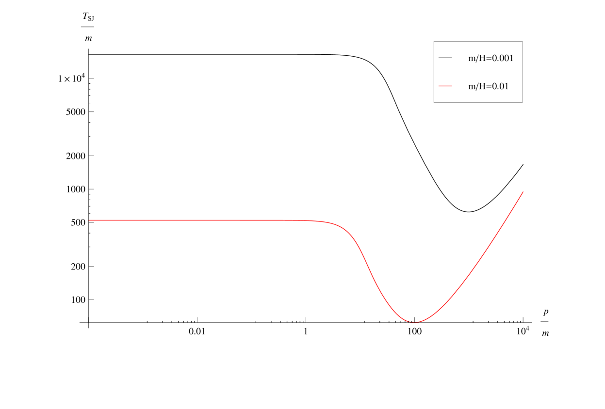
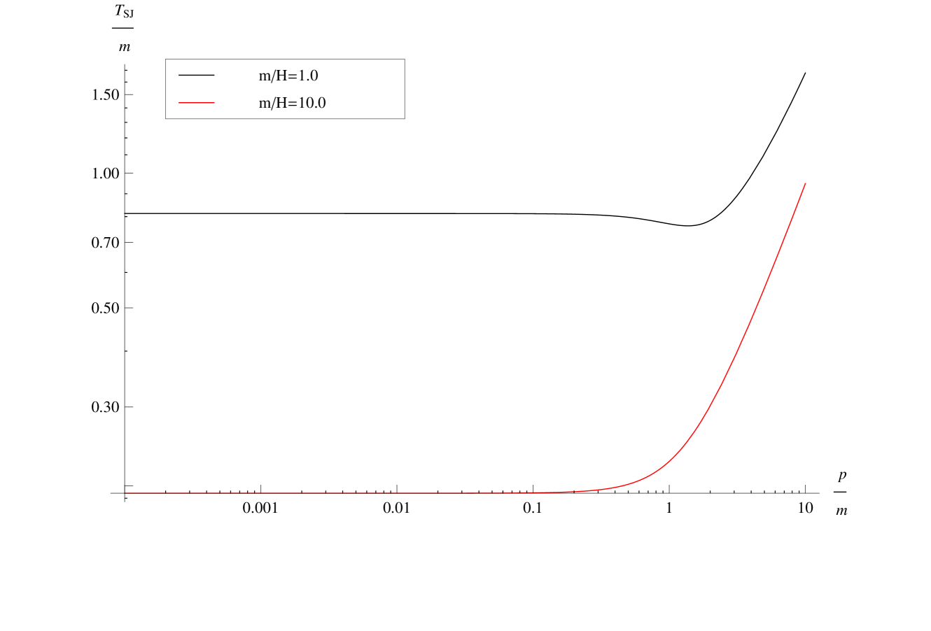
Figure 1: Behaviour of $T_{SJ}$ for different ratios of $\frac{m}{H}$ and $\frac{p}{H}$.

It is evident that the long wavelength modes are in fact at a constant effective temperature. For example, in the regime where $m\ll H$ and $p\ll\sqrt{mH}$, the Whittaker function has a simple asymptotic expansion

$$W_{\lambda,\frac{1}{4}}(z)\longrightarrow\frac{\sqrt{\pi}}{\Gamma(\frac{3}{4}-\lambda)}z^{\frac{1}{4}}-\frac{2\sqrt{\pi}}{\Gamma(\frac{1}{4}-\lambda)}z^{3/2}+\mathcal{O}(z^{5/4}),$$ (65)

using which it can be shown that

$$T_{SJ}(p)\sim\frac{\pi}{4\left|\Gamma(3/4)\right|^{2}}\frac{H^{3/2}}{\sqrt{m}}.$$ (66)

This result suggests that there are correlations on super-horizon scales. It is noteworthy that these correlations have appeared without the help of any previous epoch of accelerated expansion. Potentially, they could therefore open up a new perspective on the question of primordial fluctuations and on the related puzzle sometimes called “horizon problem”.

6 Causality and the S-J Vacuum

Like other vacuua, the S-J vacuum is defined globally, and it depends on both the causal past and future of the spacetime. Consider for example a spacetime which is first static, then expands for a short time, then goes back to being static again. In light of the inherent time-reversal symmetry of the conditions defining our vacuum-state, it is clear that this state can agree neither with the early-time vacuum (the state of minimum energy at that time), nor with the late-time vacuum. Rather, it must strike some sort of “compromise” between them.

In the present section we will illustrate this behavior with a simple example, but before doing so, we would like to dwell for a bit on the question of whether one should interpret this type of dependence on the future as a failure of causality. By construction, our definition of the vacuum depends on the full spacetime geometry. That it thereby fails to be what John Bell called “locally causal” is no surprise because, as is well understood by now, any reasonable quantum state must incorporate nonlocal correlations and entanglement. Certainly the Minkowski vacuum does so. But does this type of nonlocality also imply genuine acausality?

The prior question that begs for an answer here is what is meant by acausality in the context of quantum field theory, considering also that quantum field theory must ultimately find its place within a theory of full quantum gravity. If we remain within the “operationalist” framework of external agents, “measurements” and state-vector collapse, then causality (in the sense of relativistic causality) reduces to the impossibility of superluminal signalling. In this sense, there is no question of acausality as long as the twin conditions of spacelike commutativity and hyperbolicity of the field equations are respected, which by construction they are in the field theory we are working with in this paper. On the other hand, if we try to adopt a more “objective” framework which dispenses with external agents, then we seem to be left without any clear definition of relativistic causality at all. That is, we lack an intrinsic criterion which could decide whether or not physical influences are propagating outside the light cone or “into the past”. But without such a criterion, the meaning of relativistic causality in general is called into question.

A further observation also seems relevant here, even if it does not turn out to be decisive. Namely, the assumption we have made of a fixed, non-dynamical spacetime is already “anticausal” in a certain sense. In a full quantum gravity theory the future geometry must evolve together with, and in mutual dependence on the future matter-field. Hence, any attempt to specify the geometry in advance amounts to imposing a future boundary condition on the combined system of metric plus scalar field. Given this, it would not be surprising if a correct semiclassical treatment of the scalar were also to involve some degree of “dependence on the future”.

The specific model we will consider is a 1+1 dimensional FLRW universe with metric $ds^{2}=C(\eta)(d\eta^{2}-dx^{2})$, where $C(\eta)=A+B\tanh(\rho\eta)$. In the infinite past $C(\eta)\to A-B$ and in the infinite future $C(\eta)\to A+B$. It is known that there are normalized modes $u_{k}^{in}(\eta,x)$ that behave like positive frequency Minkowski-space modes in the remote past ($\eta,t\to-\infty$):

$$u_{k}^{in}(\eta,x) = \frac{1}{\sqrt{4\pi\omega^{in}_{k}}}e^{ikx-i\omega^{+}_{k}\eta-(i\omega^{-}_{k}/\rho)\ln[2\cosh(\rho\eta)]}$$ (67)

$$\times {}_{2}F_{1}(1+(i\omega^{-}_{k}/\rho),i\omega^{-}_{k}/\rho;1-(i\omega^{in}_{k}/\rho);\frac{1}{2}(1+\tanh(\rho\eta)))$$

$$\stackrel{{\scriptstyle\eta\to-\infty}}{{\longrightarrow}} \frac{1}{\sqrt{4\pi\omega^{in}_{k}}}e^{ikx-i\omega^{in}_{k}\eta},$$

where ${}_{2}F_{1}$ is the ordinary hypergeometric function and

$$\omega^{in}_{k} = [k^{2}+m^{2}(A-B)]^{1/2}$$

$$\omega^{out}_{k} = [k^{2}+m^{2}(A+B)]^{1/2}$$

$$\omega^{\pm}_{k} = \frac{1}{2}(\omega^{out}_{k}\pm\omega^{in}_{k}).$$ (68)

Similarly, there are normalized modes $u_{k}^{out}(\eta,x)$ that behave like the positive frequency Minkowski-space modes in the remote future: ($\eta,t\to\infty$)

$$u_{k}^{out}(\eta,x) = \frac{1}{\sqrt{4\pi\omega^{out}_{k}}}e^{ikx-i\omega^{+}_{k}\eta-(i\omega^{-}_{k}/\rho)\ln[2\cosh(\rho\eta)]}$$ (69)

$$\times {}_{2}F_{1}(1+(i\omega^{-}_{k}/\rho),i\omega^{-}_{k}/\rho;1+(i\omega^{out}_{k}/\rho);\frac{1}{2}(1-\tanh(\rho\eta)))$$

$$\stackrel{{\scriptstyle\eta\to\infty}}{{\longrightarrow}} \frac{1}{\sqrt{4\pi\omega^{out}_{k}}}e^{ikx-i\omega^{out}_{k}\eta}.$$

The in and out modes are related to eachother by the following Bogolubov transformation

$$u_{k}^{in}(\eta,x)=\alpha_{k}u_{k}^{out}(\eta,x)+\beta_{k}\bar{u}_{-k}^{out},$$ (70)

where

$$\alpha_{k} = (\frac{\omega^{out}_{k}}{\omega^{in}_{k}})^{1/2}\frac{\Gamma(1-(i\omega^{in}_{k}/\rho))\Gamma(-(i\omega^{out}_{k}/\rho))}{\Gamma(1-(i\omega^{+}_{k}/\rho))\Gamma(-i\omega^{+}_{k}/\rho)}$$ (71)

$$\beta_{k} = (\frac{\omega^{out}_{k}}{\omega^{in}_{k}})^{1/2}\frac{\Gamma(1-(i\omega^{in}_{k}/\rho))\Gamma(-(i\omega^{out}_{k}/\rho))}{\Gamma(1+(i\omega^{-}_{k}/\rho))\Gamma(i\omega^{-}_{k}/\rho)}.$$ (72)

The modes $u^{in}_{k}$ and $u^{out}_{k}$ define vacuum states at early and late times, respectively. If the system is at first ($\eta\to-\infty$) in the in-vacuum state, i.e. the no particle state, it will have $|\beta_{k}|^{2}$ particles of momentum $k$ with respect to the out-vacuum after the expansion ($\eta\to\infty$). The S-J vacuum has a different nature, simply because the vacuum state in the $\eta\to-\infty$ region depends on what happens in the infinite future (and vice-versa). We can find the S-J vacuum by substituting the modefunctions $u_{k}^{in}(\eta,x)$ in formula (25). Defining $g_{k}(\eta)$ through $u_{k}^{in}(\eta,x)=\frac{e^{ikx}}{\sqrt{2\pi}}g_{k}(\eta)$, it can be easily verified that

$$<u_{k}^{in},u_{k^{\prime}}^{in}> = \delta(k-k^{\prime})\int_{-\Lambda}^{\Lambda}\bar{g}_{k}(\eta)g_{k^{\prime}}(\eta)C(\eta)\,\mathrm{d}\eta$$ (73)

$$<\bar{u}_{k}^{in},u_{k^{\prime}}^{in}> = \delta(k+k^{\prime})\int_{-\Lambda}^{\Lambda}g_{k}(\eta)g_{k^{\prime}}(\eta)C(\eta)\,\mathrm{d}\eta,$$ (74)

where as usual, we have regulated the integrals with a cutoff $\Lambda$. The asymptotic behaviour of $g_{k}(\eta)$ is given by

$$g_{k}(\eta) \stackrel{{\scriptstyle\eta\to-\infty}}{{\longrightarrow}} \frac{1}{\sqrt{2\omega^{in}_{k}}}e^{-i\omega^{in}_{k}\eta}$$ (75)

$$g_{k}(\eta) \stackrel{{\scriptstyle\eta\to\infty}}{{\longrightarrow}} \frac{1}{\sqrt{2\omega^{out}_{k}}}(\alpha_{k}e^{-i\omega^{out}_{k}\eta}+\beta_{k}e^{i\omega^{out}_{k}\eta}).$$ (76)

Using these expressions, it can be checked that

$$\lim_{\Lambda\to\infty}\frac{<\bar{u}_{-k}^{in},u_{k}^{in}>}{<u_{k}^{in},u_{k}^{in}>}\longrightarrow\frac{2\alpha_{k}\beta_{k}}{|\alpha_{k}|^{2}+|\beta_{k}|^{2}+\frac{\omega_{out}}{\omega_{in}}\frac{A-B}{A+B}}\equiv\gamma_{k},$$ (77)

from which the S-J vacuum can be computed using (25):

$$u^{SJ}_{k}(\eta,x) = \mu_{k}u^{in}_{k}(\eta,x)+\xi_{k}\bar{u}^{in}_{-k}(\eta,x)$$ (78)

$$\mu_{k} = \frac{1}{\sqrt{2}}\left[1+\frac{1}{\sqrt{1-|\gamma_{k}|^{2}}}\right]^{\frac{1}{2}}$$ (79)

$$\xi_{k} = -\frac{1}{\sqrt{2}}\left[-1+\frac{1}{\sqrt{1-|\gamma_{k}|^{2}}}\right]^{\frac{1}{2}}e^{i\text{Arg}(\alpha_{k}\beta_{k})}.$$ (80)

Fig. 2 shows the difference between the S-J and “in” vacuua for a specific set of parameters and frequencies. As one would expect, this deviation is only significant for low-frequency modes, which are more sensitive to the rate of expansion $\rho$.

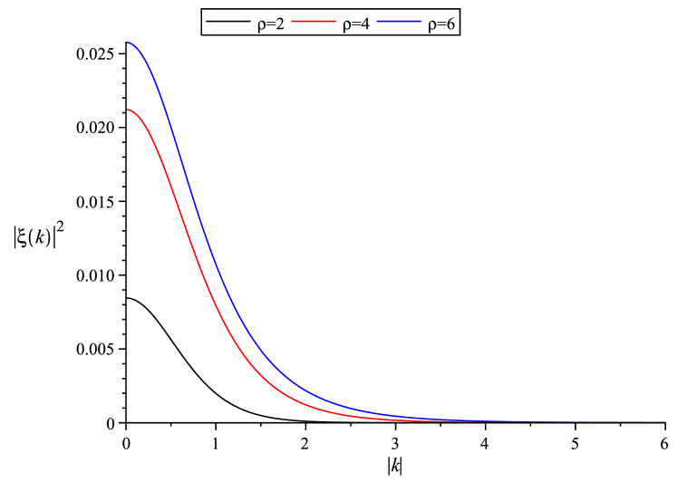
Figure 2: The deviation between the S-J and “in” vacuua, as measured by $|\xi(k)|^{2}$, defined in (80). The parameters used here are $A=2.0$, $B=1.0$, and $m=1.0$.

7 Conclusions and Discussions

We have defined a distinguished vacuum for a free quantum field in a globally hyperbolic region of an arbitrarily curved spacetime. This “S-J” state is well-defined for all compact regions and for a large class of noncompact ones.

We have shown that for static spacetimes, our vacuum coincides with the usual ground state. We have also computed it explicitly for a scalar field of mass $m\geq 0$ in a radiation-filled, spatially flat, homogeneous and isotropic cosmos. In that connection we also computed an “effective temperature that can be defined for the super-horizon modes of the massive field. The correlations found thereby could open up a new perspective on the question of primordial fluctuations and the so-called “horizon problem”.

A peculiar aspect of our prescription is its temporal non-locality. We demonstrated this feature by the example of a spacetime which sandwiches a region with curvature in-between flat initial and final regions, but we did not explore its phenomenological implications any further. In a parallel effort deSitter , we have also applied our prescription to de Sitter space, obtaining results for both the full spacetime and for the so-called Poincaré patch. The vacua obtained thereby differ from the Euclidean (Bunch-Davies) vacuum below a certain mass threshold, with potentially interesting phenomenology.

A question that we have not addressed in this paper is whether, or in which circumstances, the S-J vacuum obeys the so-called Hadamard condition. Since this work was completed, some results have appeared FV showing that the answer is yes in some cases and no in others. We hope to return to this and related matters elsewhere.

Appendix A Comments and Calculations

A.1 When is $i\Delta$ self-adjoint?

We saw in the main text that $i\Delta$ is self-adjoint and has a complete set of normalizable eigenvectors when $i\Delta(x,y)\in L^{2}(M\times M)$. In 3+1 dimensions, this Hilbert-Schmidt condition is not satisfied, however, because the retarded Green’s function is a distribution, and not a function. Nonetheless, it is still possible to show that $i\Delta$ is self-adjoint when $M$ is bounded. Here, we will show that this is indeed the case for a bounded region $M$ of Minkowski space, and will argue that this conclusion should continue to hold in all curved spacetimes.

In $3+1$ dimensional Minkowski space ($\mathbb{M}^{4}$), we have $G_{R}(x,y)=G(x-y)$ with $G(x)$ given by

$$G(x)=\theta(t)\theta(s^{2})\Big{(}\frac{\delta(s^{2})}{2\pi}-\frac{m}{4\pi s}J_{1}(ms)\Big{)},$$ (81)

where $s=\sqrt{t^{2}-\vec{x}^{2}}$ for $t^{2}\geq\vec{x}^{2}$, and $s=-i\sqrt{\vec{x}^{2}-t^{2}}$ for $t^{2}\leq\vec{x}^{2}$. $J_{1}$ is a Bessel function of the first kind and $m$ is the mass of the scalar field. We will now show that $i\Delta$ is a bounded operator on $\textrm{C}_{0}^{\infty}(M)$, i.e. we will prove that there exists $N>0$ such that $||i\Delta f||\leq N||f||$ for all $f\in\textrm{C}_{0}^{\infty}(M)$, where $||\cdot||$ is the $L^{2}(\mathbb{M}^{4})$ norm. Let $G_{R}f=\int_{M}G_{R}(x,y)f(y)\,\mathrm{d}V_{y}$ and $G_{A}f=\int_{M}G_{A}(x,y)f(y)\,\mathrm{d}V_{y}$ denote the retarded and advanced solutions of the Klein-Gordon equation with source $f$, respectively. It is enough to show that $G_{R}$ and $G_{A}$ are bounded because $||i\Delta f||=||iG_{R}f-iG_{A}f||\leq||G_{R}f||+||G_{A}f||$.

Let $A(x)=\theta(t)\theta(s^{2})\frac{\delta(s^{2})}{2\pi}$ and $B(x)=\theta(t)\theta(s^{2})\frac{m}{4\pi s}J_{1}(ms)$ so that $G(x)=A(x)-B(x)$. Then: $||G_{R}f||=||Af-Bf||\leq||Af||+||Bf||\leq||Af||+\frac{m^{2}V}{8\pi}||f||$, where V is the total spacetime volume. Therefore, $G_{R}$ is bounded if and only if $A$ is bounded. Consider a bounded region of $\mathbb{M}^{4}$ where $\vec{x}\in[\vec{x}_{min},\vec{x}_{max}]$ and $t\in[t_{min},t_{max}]$, and a smooth function of compact support $f(t,\vec{x})$ on this region. It can be shown that:

$$(Af)(t,\vec{x})=\int_{\vec{x}_{min}}^{\vec{x}_{max}}\frac{f(t-|\vec{x}-\vec{y}|,\vec{y})}{4\pi|\vec{x}-\vec{y}|}\,\mathrm{d}^{3}\vec{y}.$$ (82)

It then follows from the Cauchy-Schwarz inequality that

$$|(Af)(t,\vec{x})|^{2}\leq\frac{1}{16\pi^{2}}\Big{\{}\int_{\vec{x}_{min}}^{\vec{x}_{max}}\frac{\,\mathrm{d}^{3}\vec{y}}{|\vec{x}-\vec{y}|^{2}}\Big{\}}\times\Big{\{}\int_{\vec{x}_{min}}^{\vec{x}_{max}}|f(t-|\vec{x}-\vec{y}|,\vec{y})|^{2}\,\mathrm{d}^{3}\vec{y}\Big{\}}.$$ (83)

Also,

$$\int_{\vec{x}_{min}}^{\vec{x}_{max}}\frac{\,\mathrm{d}^{3}\vec{y}}{|\vec{x}-\vec{y}|^{2}}=\int_{\vec{x}_{min}+\vec{x}}^{\vec{x}_{max}+\vec{x}}\frac{\,\mathrm{d}^{3}\vec{y}}{|\vec{y}|^{2}}\leq\int_{2\vec{x}_{min}}^{2\vec{x}_{max}}\frac{\,\mathrm{d}^{3}\vec{y}}{|\vec{y}|^{2}}\equiv C_{0},$$ (84)

where $C_{0}$ is some finite positive number. So we have that

$$|(Af)(t,\vec{x})|^{2}\leq\frac{C_{0}}{16\pi^{2}}\Big{\{}\int_{\vec{x}_{min}}^{\vec{x}_{max}}|f(t-|\vec{x}-\vec{y}|,\vec{y})|^{2}\,\mathrm{d}^{3}\vec{y}\Big{\}}.$$ (85)

It then follows that

$$||Af||^{2} = \int_{\vec{x}_{min}}^{\vec{x}_{max}}\,\mathrm{d}^{3}\vec{x}\int_{t_{min}}^{t_{max}}\,\mathrm{d}t|(Af)(t,\vec{x})|^{2}$$ (86)

$$\leq \frac{C_{0}}{16\pi^{2}}\int_{\vec{x}_{min}}^{\vec{x}_{max}}\,\mathrm{d}^{3}\vec{x}\int_{\vec{x}_{min}}^{\vec{x}_{max}}\,\mathrm{d}^{3}\vec{y}\int_{t_{min}}^{t_{max}}\,\mathrm{d}t|f(t-|\vec{x}-\vec{y}|,\vec{y})|^{2}$$ (87)

$$= \frac{C_{0}}{16\pi^{2}}\int_{\vec{x}_{min}}^{\vec{x}_{max}}\,\mathrm{d}^{3}\vec{x}\int_{\vec{x}_{min}}^{\vec{x}_{max}}\,\mathrm{d}^{3}\vec{y}\int_{t_{min}+|\vec{x}-\vec{y}|}^{t_{max}+|\vec{x}-\vec{y}|}\,\mathrm{d}t|f(t,\vec{y})|^{2}.$$ (88)

Since $f(t,\vec{y})$ vanishes for $t>t_{max}$: $\int_{t_{min}+|\vec{x}-\vec{y}|}^{t_{max}+|\vec{x}-\vec{y}|}\,\mathrm{d}t|f(t,\vec{y})|^{2}\leq\int_{t_{min}}^{t_{max}}\,\mathrm{d}t|f(t,\vec{y})|^{2}$, from which it follows that

$$||Af||^{2}\leq\frac{C_{0}V_{s}}{16\pi^{2}}||f||^{2},$$ (89)

where $V_{s}=\int_{\vec{x}_{min}}^{\vec{x}_{max}}\,\mathrm{d}^{3}\vec{x}$ is the enclosed spatial volume. A similar analysis goes through for the advanced solution $G_{A}f$ which results in the same bound. At long last:

$$||i\Delta f||\leq\frac{V}{4\pi}\Big{(}m^{2}+2\sqrt{\frac{C_{0}V_{s}}{V^{2}}}\Big{)}||f||.$$ (90)

Because $i\Delta$ is bounded on $\textrm{C}_{0}^{\infty}(M)$ and $\textrm{C}_{0}^{\infty}(M)$ is a dense subspace of $L^{2}({M})$, $i\Delta$ can be uniquely extended to $L^{2}({M})$ as a bounded operator RS . It then follows that $i\Delta$ is self-adjoint because it is Hermitian on all of $L^{2}(M)$ RS .

It should be clear that the boundedness of $i\Delta$ has everything to do with the singularity structure of $i\Delta(x,y)$ (once we restrict ourselves to bounded spacetimes). It is not terribly unrealistic to assume that this singularity structure remains (more or less) the same in curved spacetimes. This is certainly true in the coincidence limit, if the equivalence principle is respected. Based on these arguments, we assume in this paper that $i\Delta$ is a self-adjoint operator on $L^{2}(M)$, for all bounded globally-hyperbolic spacetimes $M$.

A.2 The S-J Vacuum and the Simple Harmonic Oscillator

This simple example illustrates the technical difficulties one faces when diagonalizing $i\Delta$, and how they can be resolved. Consider a simple harmonic oscillator with unit mass and frequency $\omega$, whose position $q(t)$ satisfies $(\frac{d^{2}}{dt^{2}}+\omega^{2})q(t)=0$. The associated retarded Green’s function satisfies $(\frac{d^{2}}{dt^{2}}+\omega^{2})G_{R}(t,t^{\prime})=-\delta(t-t^{\prime})$, with $G_{R}(t,t^{\prime})=0$ for $t<t^{\prime}$. The solution to this equation is $G_{R}(t,t^{\prime})=-\theta(t-t^{\prime})\frac{\sin[\omega(t-t^{\prime})]}{\omega}$, which in turn gives

$$\Delta(t,t^{\prime}) = G_{R}(t,t^{\prime})-G_{R}(t^{\prime},t)=-\frac{\sin[\omega(t-t^{\prime})]}{\omega}$$ (91)

$$= \frac{1}{2i\omega}\big{[}e^{-i\omega(t-t^{\prime})}-e^{i\omega(t-t^{\prime})}\big{]}.$$ (92)

Taking $t\in(-\infty,\infty)$, it may be verified that, formally,

$$i\Delta e^{\pm i\omega t}=\frac{\mp\delta(0)}{2\omega}e^{\pm i\omega t}.$$ (93)

Keeping the $\delta(0)$’s around, we see that $T_{\mp}(t)=\frac{e^{\pm i\omega t}}{\sqrt{\delta(0)}}$ are orthonormal eigenfunctions of $i\Delta$ with eigenvalues $\lambda_{\pm}=\pm\frac{\delta(0)}{2\omega}$. According to our prescription, the resulting positive frequency modefunction $\mathcal{U}^{SJ}(t)=\sqrt{\lambda_{+}}T_{+}(t)=\frac{e^{-i\omega t}}{\sqrt{2\omega}}$, which is completely well defined and gives the right vacuum state: the state $|0>$ annihilated by $\widehat{a}$ which multiplies $\mathcal{U}^{SJ}(t)$ in the position operator expansion $\widehat{q}(t)=\mathcal{U}^{SJ}(t)\widehat{a}+\bar{\mathcal{U}}^{SJ}(t)\widehat{a}^{\dagger}$ is in fact the minimum energy state of the Hamiltonian. Thus the infinities appearing in the spectrum of $i\Delta$ end up being harmless. In other words, the S-J vacuum state should not depend on how $\delta(0)$ is regularized.

One regularization scheme, for example, is to first restrict to $t\in[-T,T]$, diagonalize $i\Delta$, and then take the limit $T\to\infty$ once the spectrum of $i\Delta$ has been computed. Let $u(t)=\frac{e^{-i\omega t}}{\sqrt{2\omega}}$ so that $i\Delta(t,t^{\prime})=u(t)\bar{u}(t^{\prime})-u(t)\bar{u}(t^{\prime})$. Finding the spectrum of $i\Delta$ in this case is similar to diagonalizing a two-by-two matrix. It may be confirmed that there are two eigenvalues $\lambda$ and $-\lambda$ with corresponding eigenfunctions $T_{+}$ and $\bar{T}_{+}$, where

$$T_{+}=\sqrt{\frac{<u,u>+\lambda}{2\lambda^{2}}}u(t)-\sqrt{\frac{<u,u>-\lambda}{2\lambda^{2}}}e^{-i\text{arg}(<u,\bar{u}>)}\bar{u}(t)$$ (94)

$$\lambda=\sqrt{{<u,u>}^{2}-|<u,\bar{u}>|^{2}}.$$ (95)

These expressions are completely well-defined because all the inner products are finite. The corresponding positive frequency modefunction as dictated by our prescription is then

$$\mathcal{U}^{SJ}(t)=\sqrt{\lambda}T_{+}(t)=\frac{1}{\sqrt{2}}\left\{\sqrt{1+\frac{1}{\sqrt{1-\frac{|<u,\bar{u}>|^{2}}{<u,u>^{2}}}}}u(t)-\sqrt{\frac{1}{\sqrt{1-\frac{|<u,\bar{u}>|^{2}}{<u,u>^{2}}}}-1}e^{-i\text{arg}(<u,\bar{u}>)}\bar{u}(t)\right\}.$$ (96)

In the limit $T\to\infty$, the ratio $\frac{|<u,\bar{u}>|^{2}}{<u,u>^{2}}\to 0$ and we recover $\mathcal{U}^{SJ}(t)=\frac{e^{-i\omega t}}{\sqrt{2\omega}}$.

A.3 Equation (14) as an equality between distributions

Let us show that the right and left hand sides of (14) are equal if they are integrated against a smooth test function $f\in\textrm{C}_{0}^{\infty}(M)$.

Since $\Delta f\in\textbf{S}$ for any $f\in\textrm{C}_{0}^{\infty}(M)$, we can expand out $i\Delta f$ in terms of the $u_{k}$: $i\Delta f(x)=\sum_{k}\alpha_{k}u_{k}(x)+\beta_{k}\overline{u}_{k}(x)$, where $\alpha_{k}$’s and $\beta_{k}$’s are constants. It can be verified that $\alpha_{k}=(u_{k},i\Delta f)_{KG}$ and $\beta_{k}=-(\overline{u}_{k},i\Delta f)_{KG}$. Then,

$$i\Delta f(x) = \sum_{k}(u_{k},i\Delta f)_{KG}u_{k}(x)-(\overline{u}_{k},i\Delta f)_{KG}\overline{u}_{k}(x)$$ (97)

$$= \sum_{k}\langle u_{k},f\rangle u_{k}(x)-\langle\overline{u}_{k},f\rangle\overline{u}_{k}(x)$$ (98)

$$= \int_{M}\left[\sum_{k}u_{k}(x)\overline{u}_{k}(y)-\overline{u}_{k}(x)u_{k}(y)\right]f(y)\,\mathrm{d}V_{y}.$$ (99)

A.4 Another Slant on the SJ Prescription

The following simple but useful result helps put our construction in context.

Theorem A.1.

Let $\textbf{S}_{\mathbb{C}}$ denote the set of all complex solutions of the Klein-Gordon equation. Assume there are functions $u_{i}(x)\in\textbf{S}_{\mathbb{C}}$, which together with their complex conjugates span $\textbf{S}_{\mathbb{C}}$ and satisfy

$$(u_{n},u_{m})_{KG}=\delta_{nm},\text{ }(\bar{u}_{n},\bar{u}_{m})_{KG}=-\delta_{nm},\text{ }(u_{n},\bar{u}_{m})_{KG}=0$$ (100)

$$\frac{<u_{n},u_{m}>}{<u_{n},u_{n}>}=\delta_{nm},\text{ }<u_{n},\bar{u}_{m}>=0,$$ (101)

where $<,>:\textbf{S}_{\mathbb{C}}\times\textbf{S}_{\mathbb{C}}\to\mathbb{C}$ is the $L^{2}$ inner product defined in (11). (See Section 2 for the definition of $(,)_{KG}$.) Then, any other functions $g_{n}(x)\in\textbf{S}_{\mathbb{C}}$ that also satisfy these conditions are unitarily-related to the $u_{i}(x)$ (i.e. $g_{n}(x)=\sum_{k}\alpha_{nk}u_{k}(x)$ where $\sum_{k}\bar{\alpha}_{nk}\alpha_{mk}=\delta_{nm}$).

Proof.

Suppose both $u_{n}(x)$ and $g_{n}(x)$ satisfy the above conditions and let

$$g_{n}(x)=\sum_{k}\alpha_{nk}u_{k}(x)+\beta_{nk}\bar{u}_{k}(x).$$ (102)

Requiring $(g_{n},g_{m})_{KG}=\delta_{nm}$ implies

$$\sum_{k}\bar{\alpha}_{nk}\alpha_{mk}-\bar{\beta}_{nk}\beta_{mk}=\delta_{nm}.$$ (103)

Also, it follows from (102) and (100) that

$$\alpha_{nk}=(u_{k},g_{n})_{KG},\qquad\beta_{nk}=-(\bar{u}_{k},g_{n})_{KG}.$$ (104)

Given that $\sum_{k}|g_{k})_{KG}(g_{k}|-|\overline{g}_{k})_{KG}(\overline{g}_{k}|$ is the identity operator on $\textbf{S}_{\mathbb{C}}$, it follows from (104) that

$$u_{n}(x) = \sum_{k}(g_{k},u_{n})_{KG}g_{k}(x)-(\bar{g}_{k},u_{n})_{KG}\bar{g}_{k}(x)$$ (105)

$$= \sum_{k}\bar{\alpha}_{kn}g_{k}(x)-\beta_{kn}\bar{g}_{k}(x)\ .$$

Using (102) and (101), it can also be verified that

$$\beta_{nk}=\frac{<\bar{u}_{k},g_{n}>}{<u_{k},u_{k}>}\ .$$ (106)

Similarly, (105) and the $L^{2}$ orthogonality conditions for the $g_{i}(x)$s (which amounts to replacing all $u$’s with $g$’s in (101)) imply

$$\beta_{nk}=-\frac{<\bar{g}_{n},u_{k}>}{<g_{n},g_{n}>}\ .$$ (107)

Given that $\langle\bar{u}_{k},g_{n}\rangle\,=\,\langle\bar{g}_{n},u_{k}\rangle$, $\langle u_{k},u_{k}\rangle\,>0$, and $\langle g_{n},g_{n}\rangle\,>0$, it follows from (106) and (107) that $\langle\bar{u}_{k},g_{n}\rangle\,=\,0$. This in turn implies that $\beta_{nk}=0$, which together with (103) proves the theorem. ∎

Note that this proof is valid for any Hermitian inner product $<,>$ on $\textbf{S}_{\mathbb{C}}$ which enjoys the additional property $<\bar{f},g>\,=\,<\bar{g},f>\,.$

We have shown here that requiring (101), in addition to the usual quantization conditions, is enough to define a distinguished vacuum state. That these modes are eigenfunctions of $i\Delta$ ($(i\Delta u_{n})(x)=<u_{n},u_{n}>u_{n}(x)$), follows from (14).

Appendix B Useful Theorems

Theorem B.1.

Let $(M,g_{ab})$ be a globally hyperbolic spacetime with smooth, spacelike Cauchy surface $\Sigma$. Then the Klein-Gordon equation (1) has a well posed initial value formulation in the following sense: Given any pair of smooth ($\textrm{C}^{\infty}$) functions $(\phi_{0},\dot{\phi}_{0})$ on $\Sigma$, there exists a unique solution $\phi$ to (1), defined on all of $M$, such that on $\Sigma$ we have $\phi=\phi_{0}$ and $n^{a}\nabla_{a}\phi=\dot{\phi}_{0}$, where $n^{a}$ denotes the unit (future-directed) normal to $\Sigma$. Furthermore, for any closed subset $S\subset\Sigma$, the solution, $\phi$, restricted to D(S) depends only upon the initial data on S. In addition, $\phi$ is smooth and varies continuously with the initial data.

The above theorem continues to hold if a (fixed, smooth) “source term” $f$ is inserted on the right hand side of (1). It then follows from the domain of dependence feature of the theorem that there exist unique advanced and retarded solutions to the Klein-Gordon equation with source, whence in a globally hyperbolic spacetime there exist unique advanced and retarded Green’s functions for the Klein-Gordon equation.

Theorem B.2.

$\Delta:\textrm{C}_{0}^{\infty}\to\textbf{S}$ satisfies $\int_{M}\phi f\,\mathrm{d}V=\Omega(\Delta f,\phi)$ for all $f\in\textrm{C}_{0}^{\infty}$ and $\phi\in\textbf{S}$ .

Proof.

Let’s first give a simple proof for 1+1 dimensional Minkowski space and then generalize the arguments to globally hyperbolic spacetimes of higher spatial dimension. Pick $t_{1},t_{2}\in\mathbb{R}$ such that $f=0$ for $t\notin[t_{1},t_{2}]$. Then:

$$\int_{M}\phi f\,\mathrm{d}V=\int_{t_{1}}^{t_{2}}\,\mathrm{d}t\int_{-\infty}^{\infty}\phi(\partial_{t}^{2}-\partial_{x}^{2}+m^{2})(Af)\,\mathrm{d}x,$$ (108)

where $Af$ is the advanced solution of the Klein-Gordon equation with source $f$. Now integrating by parts twice yields

$$\int_{t_{1}}^{t_{2}}\phi\partial_{t}^{2}(Af)\,\mathrm{d}t = \phi\partial_{t}(Af)|^{t_{2}}_{t_{1}}-\partial_{t}\phi(Af)|^{t_{2}}_{t_{1}}+\int_{t_{1}}^{t_{2}}(Af)\partial_{t}^{2}\phi\,\mathrm{d}t$$ (109)

$$= \partial_{t}\phi(Af)|_{t_{1}}-\phi\partial_{t}(Af)|_{t_{1}}+\int_{t_{1}}^{t_{2}}(Af)(\partial_{x}^{2}-m^{2})\phi\,\mathrm{d}t,$$ (110)

where we have used the Klein-Gordon equation and that $Af$ vanishes outside the causal past of the support of $f$. Substituting this back into (108), we can further simplify by noting that $\int_{-\infty}^{\infty}\big{[}(Af)\partial_{x}^{2}\phi-\phi\partial_{x}^{2}(Af)\big{]}\,\mathrm{d}x=0$ . (Because $Af$ induces initial data of compact support on all equal-time spatial slices, all surface terms vanish.) Using this we find:

$$\int_{M}\phi f\,\mathrm{d}V=\int_{-\infty}^{\infty}\big{[}\partial_{t}\phi(Af)|_{t_{1}}-\phi\partial_{t}(Af)|_{t_{1}}\big{]}\,\mathrm{d}x=\Omega(\Delta f,\phi),$$ (111)

since $Rf$ (the retarded solution of the Klein-Gordon equation with source $f$) vanishes at $t=t_{1}$. To generalize the proof, we write

$$\int_{M}\phi f\,\mathrm{d}V = \int_{M}\phi(\nabla_{\mu}\nabla^{\mu}+m^{2})(Af)\,\mathrm{d}V$$ (112)

$$= \int_{M}\nabla_{\mu}\{\phi\nabla^{\mu}(Af)\}\,\mathrm{d}V-\int_{M}\nabla_{\mu}\phi\nabla^{\mu}(Af)\,\mathrm{d}V+\int_{M}m^{2}\phi(Af)$$

$$= \int_{M}\nabla_{\mu}\{\phi\nabla^{\mu}(Af)-(Af)\nabla^{\mu}\phi\}\,\mathrm{d}V+\int_{M}(\nabla_{\mu}\nabla^{\mu}+m^{2})\phi(Af)\,\mathrm{d}V$$

$$= \int_{\partial M}\{\phi n^{\mu}\nabla_{\mu}(Af)-(Af)n^{\mu}\nabla_{\mu}\phi\}\sqrt{-h}\,\mathrm{d}^{3}x,$$

where we have used the Stoke’s theorem in the last line. Here $n^{\mu}$ is the unit normal to the boundary $\partial M$ and $h$ is the determinant of the induced metric on the boundary. Again, because $Af$ induces initial data of compact support on all equal-time spatial slices and $Af$ vanishes outside the causal past of the support of $f$:

$$\int_{\partial M}\{\phi n^{\mu}\nabla_{\mu}(Af)-(Af)n^{\mu}\nabla_{\mu}\phi\}\sqrt{-h}\,\mathrm{d}^{3}x = -\int_{\Sigma_{t_{1}}}\{\phi n^{\mu}\nabla_{\mu}(Af)-(Af)n^{\mu}\nabla_{\mu}\phi\}\sqrt{-h}\,\mathrm{d}^{3}x$$ (113)

$$= \Omega(\Delta f,\phi),$$

where we have used in the last line that $Rf$ vanishes at $\Sigma_{t_{1}}$. ∎

Theorem B.3.

$G_{R}(x,z)=G_{A}(z,x)$.

Proof.

Let $M$ be the region bounded by a pair of Cauchy surfaces, one to the future of both $x$ and $z$, the other to their past. Then

$$G_{R}(x,z)-G_{A}(z,x) = \int_{M}\big{\{}G_{R}(y,z)\delta^{4}(y-x)-G_{A}(y,x)\delta^{4}(y-z)\big{\}}\,\mathrm{d}^{4}y$$

$$= \int_{M}\big{\{}G_{A}(y,x)(\Box_{y}+m^{2})G_{R}(y,z)-G_{R}(y,z)(\Box_{y}+m^{2})G_{A}(y,x)\big{\}}\,\mathrm{d}V_{y}$$

$$= \int_{M}\big{\{}G_{A}(y,x)\Box_{y}G_{R}(y,z)-G_{R}(y,z)\Box_{y}G_{A}(y,x)\big{\}}\,\mathrm{d}V_{y}$$

$$= \int_{M}\nabla_{\mu}\big{\{}G_{A}(y,x)\nabla^{\mu}G_{R}(y,z)-G_{R}(y,z)\nabla^{\mu}G_{A}(y,x)\big{\}}\,\mathrm{d}V_{y}$$

$$= \int_{\partial M}\big{\{}G_{A}(y,x)n^{\mu}\nabla_{\mu}G_{R}(y,z)-G_{R}(y,z)n^{\mu}\nabla_{\mu}G_{A}(y,x)\big{\}}\sqrt{-h}\,\mathrm{d}^{3}y=0$$

where we have used the Stoke’s theorem in the last line. Here $n^{\mu}$ is the unit normal to the boundary $\partial M$ and $h$ is the determinant of the induced metric on the boundary. We now explain why the last expression is identically zero. By definition, it is only when $y$ is in the causal future of $z$ and the causal past of $x$ where this expression could be nonzero. However, because $y$ is being evaluated at the boundary this is never possible in a globally hyperbolic spacetime. ∎

References

- (1) S. Johnston, Feynman propagator for a free scalar field on a causal set, Phys. Rev. Lett. 103 (Oct, 2009) 180401.
- (2) R. D. Sorkin, Scalar field theory on a causal set in histories form, Journal of Physics: Conference Series 306 (2011), no. 1 012017.
- (3) S. Hawking, Particle creation by black holes, Communications in Mathematical Physics 43 (1975) 199–220. 10.1007/BF02345020.
- (4) J. J. Bisognano and E. H. Wichmann, On the duality condition for a hermitian scalar field, Journal of Mathematical Physics 16 (1975), no. 4 985–1007.
- (5) W. G. Unruh, Notes on black-hole evaporation, Phys. Rev. D 14 (Aug, 1976) 870–892.
- (6) V. F. Mukhanov, H. A. Feldman, and R. H. Brandenberger, Theory of cosmological perturbations, Physics Reports 215 (1992), no. 5-6 203 – 333.
- (7) B. Allen, Vacuum states in de sitter space, Physical Review D 32 (1985) 3136–3149.
- (8) R. Wald, Quantum field theory in curved spacetime and black hole thermodynamics. Chicago lectures in physics. University of Chicago Press, 1994.
- (9) R. M. Wald, The Formulation of Quantum Field Theory in Curved Spacetime, arXiv:0907.0416.
- (10) F. Dowker, S. Johnston, and R. D. Sorkin, Hilbert spaces from path integrals, Journal of Physics A: Mathematical and Theoretical 43 (2010), no. 27 275302, [arXiv:1002.0589].
- (11) R. D. Sorkin, Quantum mechanics as quantum measure theory, Mod.Phys.Lett. A9 (1994) 3119–3128, [gr-qc/9401003].
- (12) R. D. Sorkin, Toward a ’fundamental theorem of quantal measure theory’, arXiv:1104.0997.
- (13) J. B. Hartle, Space-time quantum mechanics and the quantum mechanics of space-time, gr-qc/9304006. 183pages, UCSB92-21, (corrected macro calls) Journal-ref: in Gravitation and Quantizations: Proceedings of the 1992 Les Houches Summer School, ed. by B. Julia and J. Zinn-Justin, North Holland, Amsterdam, 1995.
- (14) A. Ashtekar and A. Magnon-Ashtekar, A curiosity concerning the role of coherent states in quantum field theory, Pramana 15 (1980) 107–115. 10.1007/BF02847917.
- (15) M. Reed and B. Simon, I: Functional Analysis, Volume 1 (Methods of Modern Mathematical Physics) (vol 1). Academic Press, rev enl su ed., Jan., 1981.
- (16) C. J. Fewster and R. Verch, On a Recent Construction of ’Vacuum-like’ Quantum Field States in Curved Spacetime, arXiv:1206.1562.
- (17) N. Afshordi, M. Buck, F. Dowker, D. Rideout, R. D. Sorkin, et al., A Ground State for the Causal Diamond in 2 Dimensions, arXiv:1207.7101.
- (18) N. Afshordi, S. Aslanbeigi, M. Buck, F. Dowker, and R. Sorkin. In preparation.
- (19) S. Fulling, Remarks on positive frequency and hamiltonians in expanding universes, General Relativity and Gravitation 10 (1979) 807–824. 10.1007/BF00756661.
- (20) C. Dappiaggi, T.-P. Hack, and N. Pinamonti, Approximate KMS states for scalar and spinor fields in Friedmann-Robertson-Walker spacetimes, Annales Henri Poincare 12 (2011) 1449–1489, [arXiv:1009.5179].
- (21) N. Birrell and P. Davies, Quantum Fields in Curved Space. Cambridge University Press, Cambridge, 1982.
- (22) F. W. Olver, D. W. Lozier, R. F. Boisvert, and C. W. Clark, NIST Handbook of Mathematical Functions. Cambridge University Press, New York, NY, USA, 1st ed., 2010.