LP-rounding Algorithms for the Fault-Tolerant
Facility Placement Problem

Abstract

The Fault-Tolerant Facility Placement problem (FTFP) is a generalization of the classic Uncapacitated Facility Location Problem (UFL). In FTFP we are given a set of facility sites and a set of clients. Opening a facility at site $i$ costs $f_{i}$ and connecting client $j$ to a facility at site $i$ costs $d_{ij}$. We assume that the connection costs (distances) $d_{ij}$ satisfy the triangle inequality. Multiple facilities can be opened at any site. Each client $j$ has a demand $r_{j}$, which means that it needs to be connected to $r_{j}$ different facilities (some of which could be located on the same site). The goal is to minimize the sum of facility opening cost and connection cost.

The main result of this paper is a $1.575$-approximation algorithm for FTFP, based on LP-rounding. The algorithm first reduces the demands to values polynomial in the number of sites. Then it uses a technique that we call adaptive partitioning, which partitions the instance by splitting clients into unit demands and creating a number of (not yet opened) facilities at each site. It also partitions the optimal fractional solution to produce a fractional solution for this new instance. The partitioned fractional solution satisfies a number of properties that allow us to exploit existing LP-rounding methods for UFL to round our partitioned solution to an integral solution, preserving the approximation ratio. In particular, our $1.575$-approximation algorithm is based on the ideas from the $1.575$-approximation algorithm for UFL by Byrka et al., with changes necessary to satisfy the fault-tolerance requirement.

1 Introduction

In the Fault-Tolerant Facility Placement problem (FTFP), we are given a set $\mathbb{F}$ of sites at which facilities can be built, and a set $\mathbb{C}$ of clients with some demands that need to be satisfied by different facilities. A client $j\in\mathbb{C}$ has demand $r_{j}$. Building one facility at a site $i\in\mathbb{F}$ incurs a cost $f_{i}$, and connecting one unit of demand from client $j$ to a facility at site $i$ costs $d_{ij}$. Throughout the paper we assume that the connection costs (distances) $d_{ij}$ form a metric, that is, they are symmetric and satisfy the triangle inequality. In a feasible solution, some number of facilities, possibly zero, are opened at each site $i$, and demands from each client are connected to those open facilities, with the constraint that demands from the same client have to be connected to different facilities. Note that any two facilities at the same site are considered different.

It is easy to see that if all $r_{j}=1$ then FTFP reduces to the classic Uncapacitated Facility Location problem (UFL). If we add a constraint that each site can have at most one facility built on it, then the problem becomes equivalent to the Fault-Tolerant Facility Location problem (FTFL). One implication of the one-facility-per-site restriction in FTFL is that $\max_{j\in\mathbb{C}}r_{j}\leq|\mathbb{F}|$, while in FTFP the values of $r_{j}$’s can be much bigger than $|\mathbb{F}|$.

The UFL problem has a long history; in particular, great progress has been achieved in the past two decades in developing techniques for designing constant-ratio approximation algorithms for UFL. Shmoys, Tardos and Aardal [16] proposed an approach based on LP-rounding, that they used to achieve a ratio of 3.16. This was then improved by Chudak [5] to 1.736, and later by Sviridenko [17] to 1.582. The best known “pure” LP-rounding algorithm is due to Byrka et al. [3] with ratio 1.575. Byrka and Aardal [2] gave a hybrid algorithm that combines LP-rounding and dual-fitting (based on [10]), achieving a ratio of 1.5. Recently, Li [13] showed that, with a more refined analysis and randomizing the scaling parameter used in [2], the ratio can be improved to 1.488. This is the best known approximation result for UFL. Other techniques include the primal-dual algorithm with ratio 3 by Jain and Vazirani [11], the dual fitting method by Jain et al. [10] that gives ratio 1.61, and a local search heuristic by Arya et al. [1] with approximation ratio 3. On the hardness side, UFL is easily shown to be NP-hard, and it is known that it is not possible to approximate UFL in polynomial time with ratio less than $1.463$, provided that ${\mbox{\sf NP}}\not\subseteq{\mbox{\sf DTIME}}(n^{O(\log\log n)})$ [6]. An observation by Sviridenko strengthened the underlying assumption to ${\mbox{\sf P}}\neq{\mbox{\sf NP}}$ (see [19]).

FTFL was first introduced by Jain and Vazirani [12] and they adapted their primal-dual algorithm for UFL to obtain a ratio of $3\ln(\max_{j\in\mathbb{C}}r_{j})$. All subsequently discovered constant-ratio approximation algorithms use variations of LP-rounding. The first such algorithm, by Guha et al. [7], adapted the approach for UFL from [16]. Swamy and Shmoys [18] improved the ratio to $2.076$ using the idea of pipage rounding introduced in [17]. Most recently, Byrka et al. [4] improved the ratio to 1.7245 using dependent rounding and laminar clustering.

FTFP is a natural generalization of UFL. It was first studied by Xu and Shen [20], who extended the dual-fitting algorithm from [10] to give an approximation algorithm with a ratio claimed to be $1.861$. However their algorithm runs in polynomial time only if $\max_{j\in\mathbb{C}}r_{j}$ is polynomial in $O(|\mathbb{F}|\cdot|\mathbb{C}|)$ and the analysis of the performance guarantee in [20] is flawed. To date, the best approximation ratio for FTFP in the literature is $3.16$, established by Yan and Chrobak [21], while the only known lower bound is the $1.463$ lower bound for UFL from [6], as UFL is a special case of FTFP. If all demand values $r_{j}$ are equal, the problem can be solved by simple scaling and applying LP-rounding algorithms for UFL. This does not affect the approximation ratio, thus achieving ratio $1.575$ for this special case (see also [14]).

The main result of this paper is an LP-rounding algorithm for FTFP with approximation ratio 1.575, matching the best ratio for UFL achieved via the LP-rounding method [3] and significantly improving our earlier bound in [21]. In Section 3 we prove that, for the purpose of LP-based approximations, the general FTFP problem can be reduced to the restricted version where all demand values are polynomial in the number of sites. This demand reduction trick itself gives us a ratio of $1.7245$, since we can then treat an instance of FTFP as an instance of FTFL by creating a sufficient (but polynomial) number of facilities at each site, and then using the algorithm from [4] to solve the FTFL instance.

The reduction to polynomial demands suggests an approach where clients’ demands are split into unit demands. These unit demands can be thought of as “unit-demand clients”, and a natural approach would be to adapt LP-rounding methods from [8, 5, 3] to this new set of unit-demand clients. Roughly, these algorithms iteratively pick a client that minimizes a certain cost function (that varies for different algorithms) and open one facility in the neighborhood of this client. The remaining clients are then connected to these open facilities. In order for this to work, we also need to convert the optimal fractional solution $(\boldsymbol{x}^{\ast},\boldsymbol{y}^{\ast})$ of the original instance into a solution $(\bar{\boldsymbol{x}},\bar{\boldsymbol{y}})$ of the modified instance which then can be used in the LP-rounding process. This can be thought of as partitioning the fractional solution, as each connection value $x^{\ast}_{ij}$ must be divided between the $r_{j}$ unit demands of client $j$ in some way. In Section 4 we formulate a set of properties required for this partitioning to work. For example, one property guarantees that we can connect demands to facilities so that two demands from the same client are connected to different facilities. Then we present our adaptive partitioning technique that computes a partitioning with all the desired properties. Using adaptive partitioning we were able to extend the algorithms for UFL from [8, 5, 3] to FTFP. We illustrate the fundamental ideas of our approach in Section 5, showing how they can be used to design an LP-rounding algorithm with ratio $3$. In Section 6 we refine the algorithm to improve the approximation ratio to $1+2/e\approx 1.736$. Finally, in Section 7, we improve it even further to $1.575$ – the main result of this paper.

Summarizing, our contributions are two-fold: One, we show that the existing LP-rounding algorithms for UFL can be extended to a much more general problem FTFP, retaining the approximation ratio. We believe that, should even better LP-rounding algorithms be developed for UFL in the future, using our demand reduction and adaptive partitioning methods, it should be possible to extend them to FTFP. In fact, some improvement of the ratio should be achieved by randomizing the scaling parameter $\gamma$ used in our algorithm, as Li showed in [13] for UFL. (Since the ratio $1.488$ for UFL in [13] uses also dual-fitting algorithms [15], we would not obtain the same ratio for FTFP yet using only LP-rounding.)

Two, our ratio of $1.575$ is significantly better than the best currently known ratio of $1.7245$ for the closely-related FTFL problem. This suggests that in the fault-tolerant scenario the capability of creating additional copies of facilities on the existing sites makes the problem easier from the point of view of approximation.

2 The LP Formulation

The FTFP problem has a natural Integer Programming (IP) formulation. Let $y_{i}$ represent the number of facilities built at site $i$ and let $x_{ij}$ represent the number of connections from client $j$ to facilities at site $i$. If we relax the integrality constraints, we obtain the following LP:

$$\textrm{minimize}\quad{\it cost}(\boldsymbol{x},\boldsymbol{y}) =\textstyle{\sum_{i\in\mathbb{F}}f_{i}y_{i}+\sum_{i\in\mathbb{F},j\in\mathbb{C}}d_{ij}x_{ij}}$$ (1)

$$\textrm{subject to}\quad y_{i}-x_{ij} \geq 0 \forall i\in\mathbb{F},j\in\mathbb{C}$$

$$\textstyle{\sum_{i\in\mathbb{F}}x_{ij}} \geq r_{j} \forall j\in\mathbb{C}$$

$$x_{ij}\geq 0,y_{i} \geq 0 \forall i\in\mathbb{F},j\in\mathbb{C}$$

The dual program is:

$$\textrm{maximize}\quad\textstyle{\sum_{j\in\mathbb{C}}}r_{j}\alpha_{j}$$ (2)

$$\textrm{subject to}\quad\textstyle{\sum_{j\in\mathbb{C}}\beta_{ij}} \leq f_{i} \forall i\in\mathbb{F}$$

$$\alpha_{j}-\beta_{ij} \leq d_{ij} \forall i\in\mathbb{F},j\in\mathbb{C}$$

$$\alpha_{j}\geq 0,\beta_{ij} \geq 0 \forall i\in\mathbb{F},j\in\mathbb{C}$$

In each of our algorithms we will fix some optimal solutions of the LPs (1) and (2) that we will denote by $(\boldsymbol{x}^{\ast},\boldsymbol{y}^{\ast})$ and $(\boldsymbol{\alpha}^{\ast},\boldsymbol{\beta}^{\ast})$, respectively.

With $(\boldsymbol{x}^{\ast},\boldsymbol{y}^{\ast})$ fixed, we can define the optimal facility cost as $F^{\ast}=\sum_{i\in\mathbb{F}}f_{i}y_{i}^{\ast}$ and the optimal connection cost as $C^{\ast}=\sum_{i\in\mathbb{F},j\in\mathbb{C}}d_{ij}x_{ij}^{\ast}$. Then $\mbox{\rm LP}^{\ast}={\it cost}(\boldsymbol{x}^{\ast},\boldsymbol{y}^{\ast})=F^{\ast}+C^{\ast}$ is the joint optimal value of (1) and (2). We can also associate with each client $j$ its fractional connection cost $C^{\ast}_{j}=\sum_{i\in\mathbb{F}}d_{ij}x_{ij}^{\ast}$. Clearly, $C^{\ast}=\sum_{j\in\mathbb{C}}C^{\ast}_{j}$. Throughout the paper we will use notation OPT for the optimal integral solution of (1). OPT is the value we wish to approximate, but, since $\mbox{\rm OPT}\geq\mbox{\rm LP}^{\ast}$, we can instead use $\mbox{\rm LP}^{\ast}$ to estimate the approximation ratio of our algorithms.

Completeness and facility splitting.

Define $(\boldsymbol{x}^{\ast},\boldsymbol{y}^{\ast})$ to be complete if $x_{ij}^{\ast}>0$ implies that $x_{ij}^{\ast}=y_{i}^{\ast}$ for all $i,j$. In other words, each connection either uses a site fully or not at all. As shown by Chudak and Shmoys [5], we can modify the given instance by adding at most $|\mathbb{C}|$ sites to obtain an equivalent instance that has a complete optimal solution, where “equivalent” means that the values of $F^{\ast}$, $C^{\ast}$ and $\mbox{\rm LP}^{\ast}$, as well as OPT, are not affected. Roughly, the argument is this: We notice that, without loss of generality, for each client $k$ there exists at most one site $i$ such that $0<x_{ik}^{\ast}<y_{i}^{\ast}$. We can then perform the following facility splitting operation on $i$: introduce a new site $i^{\prime}$, let $y^{\ast}_{i^{\prime}}=y^{\ast}_{i}-x^{\ast}_{ik}$, redefine $y^{\ast}_{i}$ to be $x^{\ast}_{ik}$, and then for each client $j$ redistribute $x^{\ast}_{ij}$ so that $i$ retains as much connection value as possible and $i^{\prime}$ receives the rest. Specifically, we set

$$y^{\ast}_{i^{\prime}}\;{\,\leftarrow\,}\;y^{\ast}_{i}-x^{\ast}_{ik},\;y^{\ast}_{i}\;{\,\leftarrow\,}\;x^{\ast}_{ik},\quad\text{ and }$$

$$x^{\ast}_{i^{\prime}j}\;{\,\leftarrow\,}\;\max(x^{\ast}_{ij}-x^{\ast}_{ik},0),\;x^{\ast}_{ij}\;{\,\leftarrow\,}\;\min(x^{\ast}_{ij},x^{\ast}_{ik})\quad\textrm{for all}\ j\neq k.$$

This operation eliminates the partial connection between $k$ and $i$ and does not create any new partial connections. Each client can split at most one site and hence we shall have at most $|\mathbb{C}|$ more sites.

By the above paragraph, without loss of generality we can assume that the optimal fractional solution $(\boldsymbol{x}^{\ast},\boldsymbol{y}^{\ast})$ is complete. This assumption will in fact greatly simplify some of the arguments in the paper. Additionally, we will frequently use the facility splitting operation described above in our algorithms to obtain fractional solutions with desirable properties.

3 Reduction to Polynomial Demands

This section presents a demand reduction trick that reduces the problem for arbitrary demands to a special case where demands are bounded by $|\mathbb{F}|$, the number of sites. (The formal statement is a little more technical – see Theorem 2.) Our algorithms in the sections that follow process individual demands of each client one by one, and thus they critically rely on the demands being bounded polynomially in terms of $|\mathbb{F}|$ and $|\mathbb{C}|$ to keep the overall running time polynomial.

The reduction is based on an optimal fractional solution $(\boldsymbol{x}^{\ast},\boldsymbol{y}^{\ast})$ of LP (1). From the optimality of this solution, we can also assume that $\sum_{i\in\mathbb{F}}x^{\ast}_{ij}=r_{j}$ for all $j\in\mathbb{C}$. As explained in Section 2, we can assume that $(\boldsymbol{x}^{\ast},\boldsymbol{y}^{\ast})$ is complete, that is $x^{\ast}_{ij}>0$ implies $x^{\ast}_{ij}=y^{\ast}_{i}$ for all $i,j$. We split this solution into two parts, namely $(\boldsymbol{x}^{\ast},\boldsymbol{y}^{\ast})=(\hat{\boldsymbol{x}},\hat{\boldsymbol{y}})+(\dot{\boldsymbol{x}},\dot{\boldsymbol{y}})$, where

$${\hat{y}}_{i} \;{\,\leftarrow\,}\;{\lfloor y_{i}^{\ast}\rfloor},\quad{\hat{x}}_{ij}\;{\,\leftarrow\,}\;{\lfloor x_{ij}^{\ast}\rfloor}\quad\textrm{and}$$

$${\dot{y}}_{i} \;{\,\leftarrow\,}\;y_{i}^{\ast}-{\lfloor y_{i}^{\ast}\rfloor},\quad{\dot{x}}_{ij}\;{\,\leftarrow\,}\;x_{ij}^{\ast}-{\lfloor x_{ij}^{\ast}\rfloor}$$

for all $i,j$. Now we construct two FTFP instances ${\hat{\cal I}}$ and ${\dot{\cal I}}$ with the same parameters as the original instance, except that the demand of each client $j$ is ${\hat{r}}_{j}=\sum_{i\in\mathbb{F}}{\hat{x}}_{ij}$ in instance ${\hat{\cal I}}$ and ${\dot{r}}_{j}=\sum_{i\in\mathbb{F}}{\dot{x}}_{ij}=r_{j}-{\hat{r}}_{j}$ in instance ${\dot{\cal I}}$. It is obvious that if we have integral solutions to both ${\hat{\cal I}}$ and ${\dot{\cal I}}$ then, when added together, they form an integral solution to the original instance. Moreover, we have the following lemma.

Lemma 1.

(i) $(\hat{\boldsymbol{x}},\hat{\boldsymbol{y}})$ is a feasible integral solution to instance ${\hat{\cal I}}$.

(ii) $(\dot{\boldsymbol{x}},\dot{\boldsymbol{y}})$ is a feasible fractional solution to instance ${\dot{\cal I}}$.

(iii) ${\dot{r}}_{j}\leq|\mathbb{F}|$ for every client $j$.

Proof.

(i) For feasibility, we need to verify that the constraints of LP (1) are satisfied. Directly from the definition, we have ${\hat{r}}_{j}=\sum_{i\in\mathbb{F}}{\hat{x}}_{ij}$. For any $i$ and $j$, by the feasibility of $(\boldsymbol{x}^{\ast},\boldsymbol{y}^{\ast})$ we have ${\hat{x}}_{ij}={\lfloor x_{ij}^{\ast}\rfloor}\leq{\lfloor y^{\ast}_{i}\rfloor}={\hat{y}}_{i}$.

(ii) From the definition, we have ${\dot{r}}_{j}=\sum_{i\in\mathbb{F}}{\dot{x}}_{ij}$. It remains to show that ${\dot{y}}_{i}\geq{\dot{x}}_{ij}$ for all $i,j$. If $x_{ij}^{\ast}=0$, then ${\dot{x}}_{ij}=0$ and we are done. Otherwise, by completeness, we have $x_{ij}^{\ast}=y_{i}^{\ast}$. Then ${\dot{y}}_{i}=y_{i}^{\ast}-{\lfloor y_{i}^{\ast}\rfloor}=x_{ij}^{\ast}-{\lfloor x_{ij}^{\ast}\rfloor}={\dot{x}}_{ij}$.

(iii) From the definition of ${\dot{x}}_{ij}$ we have ${\dot{x}}_{ij}<1$. Then the bound follows from the definition of ${\dot{r}}_{j}$. ∎

Notice that our construction relies on the completeness assumption; in fact, it is easy to give an example where $(\dot{\boldsymbol{x}},\dot{\boldsymbol{y}})$ would not be feasible if we used a non-complete optimal solution $(\boldsymbol{x}^{\ast},\boldsymbol{y}^{\ast})$. Note also that the solutions $(\hat{\boldsymbol{x}},\hat{\boldsymbol{y}})$ and $(\dot{\boldsymbol{x}},\dot{\boldsymbol{y}})$ are in fact optimal for their corresponding instances, for if a better solution to ${\hat{\cal I}}$ or ${\dot{\cal I}}$ existed, it could give us a solution to $\mathcal{I}$ with a smaller objective value.

Theorem 2.

Suppose that there is a polynomial-time algorithm ${\cal A}$ that, for any instance of FTFP with maximum demand bounded by $|\mathbb{F}|$, computes an integral solution that approximates the fractional optimum of this instance within factor $\rho\geq 1$. Then there is a $\rho$-approximation algorithm ${\cal A}^{\prime}$ for FTFP.

Proof.

Given an FTFP instance with arbitrary demands, Algorithm ${\cal A}^{\prime}$ works as follows: it solves the LP (1) to obtain a fractional optimal solution $(\boldsymbol{x}^{\ast},\boldsymbol{y}^{\ast})$, then it constructs instances ${\hat{\cal I}}$ and ${\dot{\cal I}}$ described above, applies algorithm ${\cal A}$ to ${\dot{\cal I}}$, and finally combines (by adding the values) the integral solution $(\hat{\boldsymbol{x}},\hat{\boldsymbol{y}})$ of ${\hat{\cal I}}$ and the integral solution of ${\dot{\cal I}}$ produced by ${\cal A}$. This clearly produces a feasible integral solution for the original instance $\mathcal{I}$. The solution produced by ${\cal A}$ has cost at most $\rho\cdot{\it cost}(\dot{\boldsymbol{x}},\dot{\boldsymbol{y}})$, because $(\dot{\boldsymbol{x}},\dot{\boldsymbol{y}})$ is feasible for ${\dot{\cal I}}$. Thus the cost of ${\cal A}^{\prime}$ is at most

$${\it cost}(\hat{\boldsymbol{x}},\hat{\boldsymbol{y}})+\rho\cdot{\it cost}(\dot{\boldsymbol{x}},\dot{\boldsymbol{y}})\leq\rho({\it cost}(\hat{\boldsymbol{x}},\hat{\boldsymbol{y}})+{\it cost}(\dot{\boldsymbol{x}},\dot{\boldsymbol{y}}))=\rho\cdot\mbox{\rm LP}^{\ast}\leq\rho\cdot\mbox{\rm OPT},$$

where the first inequality follows from $\rho\geq 1$. This completes the proof. ∎

4 Adaptive Partitioning

In this section we develop our second technique, which we call adaptive partitioning. Given an FTFP instance and an optimal fractional solution $(\boldsymbol{x}^{\ast},\boldsymbol{y}^{\ast})$ to LP (1), we split each client $j$ into $r_{j}$ individual unit demand points (or just demands), and we split each site $i$ into no more than $|\mathbb{F}|+2R|\mathbb{C}|^{2}$ facility points (or facilities), where $R=\max_{j\in\mathbb{C}}r_{j}$. We denote the demand set by $\overline{\mathbb{C}}$ and the facility set by $\overline{\mathbb{F}}$, respectively. We will also partition $(\boldsymbol{x}^{\ast},\boldsymbol{y}^{\ast})$ into a fractional solution $(\bar{\boldsymbol{x}},\bar{\boldsymbol{y}})$ for the split instance. We will typically use symbols $\nu$ and $\mu$ to index demands and facilities respectively, that is $\bar{\boldsymbol{x}}=({\bar{x}}_{\mu\nu})$ and $\bar{\boldsymbol{y}}=({\bar{y}}_{\mu})$. As before, the neighborhood of a demand $\nu$ is ${\overline{N}}(\nu)={\left\{\mu\in\overline{\mathbb{F}}{\,:\,}{\bar{x}}_{\mu\nu}>0\right\}}$. We will use notation $\nu\in j$ to mean that $\nu$ is a demand of client $j$; similarly, $\mu\in i$ means that facility $\mu$ is on site $i$. Different demands of the same client (that is, $\nu,\nu^{\prime}\in j$) are called siblings. Further, we use the convention that $f_{\mu}=f_{i}$ for $\mu\in i$, $\alpha_{\nu}^{\ast}=\alpha_{j}^{\ast}$ for $\nu\in j$ and $d_{\mu\nu}=d_{\mu j}=d_{ij}$ for $\mu\in i$ and $\nu\in j$. We define $C^{{\mbox{\scriptsize\rm avg}}}_{\nu}=\sum_{\mu\in{\overline{N}}(\nu)}d_{\mu\nu}{\bar{x}}_{\mu\nu}=\sum_{\mu\in\overline{\mathbb{F}}}d_{\mu\nu}{\bar{x}}_{\mu\nu}$. One can think of $C^{{\mbox{\scriptsize\rm avg}}}_{\nu}$ as the average connection cost of demand $\nu$, if we chose a connection to facility $\mu$ with probability ${\bar{x}}_{\mu\nu}$. In our partitioned fractional solution we guarantee for every $\nu$ that $\sum_{\mu\in\overline{\mathbb{F}}}{\bar{x}}_{\mu\nu}=1$.

Some demands in $\overline{\mathbb{C}}$ will be designated as primary demands and the set of primary demands will be denoted by $P$. By definition we have $P\subseteq\overline{\mathbb{C}}$. In addition, we will use the overlap structure between demand neighborhoods to define a mapping that assigns each demand $\nu\in\overline{\mathbb{C}}$ to some primary demand $\kappa\in P$. As shown in the rounding algorithms in later sections, for each primary demand we guarantee exactly one open facility in its neighborhood, while for a non-primary demand, there is constant probability that none of its neighbors open. In this case we estimate its connection cost by the distance to the facility opened in its assigned primary demand’s neighborhood. For this reason the connection cost of a primary demand must be “small” compared to the non-primary demands assigned to it. We also need sibling demands assigned to different primary demands to satisfy the fault-tolerance requirement. Specifically, this partitioning will be constructed to satisfy a number of properties that are detailed below.

(PS) Partitioned solution. Vector $(\bar{\boldsymbol{x}},\bar{\boldsymbol{y}})$ is a partition of $(\boldsymbol{x}^{\ast},\boldsymbol{y}^{\ast})$, with unit-value demands, that is:

1. $\sum_{\mu\in\overline{\mathbb{F}}}{\bar{x}}_{\mu\nu}=1$ for each demand $\nu\in\overline{\mathbb{C}}$.

2. $\sum_{\mu\in i,\nu\in j}{\bar{x}}_{\mu\nu}=x^{\ast}_{ij}$ for each site $i\in\mathbb{F}$ and client $j\in\mathbb{C}$.

3. $\sum_{\mu\in i}{\bar{y}}_{\mu}=y^{\ast}_{i}$ for each site $i\in\mathbb{F}$.

(CO) Completeness. Solution $(\bar{\boldsymbol{x}},\bar{\boldsymbol{y}})$ is complete, that is ${\bar{x}}_{\mu\nu}\neq 0$ implies ${\bar{x}}_{\mu\nu}={\bar{y}}_{\mu}$, for all $\mu\in\overline{\mathbb{F}},\nu\in\overline{\mathbb{C}}$.

(PD) Primary demands. Primary demands satisfy the following conditions:

1. For any two different primary demands $\kappa,\kappa^{\prime}\in P$ we have ${\overline{N}}(\kappa)\cap{\overline{N}}(\kappa^{\prime})=\emptyset$.

2. For each site $i\in\mathbb{F}$, $\sum_{\mu\in i}\sum_{\kappa\in P}{\bar{x}}_{\mu\kappa}\leq y_{i}^{\ast}$.

3. Each demand $\nu\in\overline{\mathbb{C}}$ is assigned to one primary demand $\kappa\in P$ such that

   1. ${\overline{N}}(\nu)\cap{\overline{N}}(\kappa)\neq\emptyset$, and

   2. $C^{{\mbox{\scriptsize\rm avg}}}_{\nu}+\alpha_{\nu}^{\ast}\geq C^{{\mbox{\scriptsize\rm avg}}}_{\kappa}+\alpha_{\kappa}^{\ast}$.

(SI) Siblings. For any pair $\nu,\nu^{\prime}$ of different siblings we have

1. ${\overline{N}}(\nu)\cap{\overline{N}}(\nu^{\prime})=\emptyset$.

2. If $\nu$ is assigned to a primary demand $\kappa$ then ${\overline{N}}(\nu^{\prime})\cap{\overline{N}}(\kappa)=\emptyset$. In particular, by Property (PD.3(a)), this implies that different sibling demands are assigned to different primary demands.

As we shall demonstrate in later sections, these properties allow us to extend known UFL rounding algorithms to obtain an integral solution to our FTFP problem with a matching approximation ratio. Our partitioning is “adaptive” in the sense that it is constructed one demand at a time, and the connection values for the demands of a client depend on the choice of earlier demands, of this or other clients, and their connection values. We would like to point out that the adaptive partitioning process for the $1.575$-approximation algorithm (Section 7) is more subtle than that for the $3$-apprximation (Section 5) and the $1.736$-approximation algorithms (Section 6), due to the introduction of close and far neighborhood.

Implementation of Adaptive Partitioning.

We now describe an algorithm for partitioning the instance and the fractional solution so that the properties (PS), (CO), (PD), and (SI) are satisfied. Recall that $\overline{\mathbb{F}}$ and $\overline{\mathbb{C}}$, respectively, denote the sets of facilities and demands that will be created in this stage, and $(\bar{\boldsymbol{x}},\bar{\boldsymbol{y}})$ is the partitioned solution to be computed.

The adaptive partitioning algorithm consists of two phases: Phase 1 is called the partitioning phase and Phase 2 is called the augmenting phase. Phase 1 is done in iterations, where in each iteration we find the “best” client $j$ and create a new demand $\nu$ out of it. This demand either becomes a primary demand itself, or it is assigned to some existing primary demand. We call a client $j$ exhausted when all its $r_{j}$ demands have been created and assigned to some primary demands. Phase 1 completes when all clients are exhausted. In Phase 2 we ensure that every demand has a total connection values ${\bar{x}}_{\mu\nu}$ equal to $1$, that is condition (PS.1).

For each site $i$ we will initially create one “big” facility $\mu$ with initial value ${\bar{y}}_{\mu}=y^{\ast}_{i}$. While we partition the instance, creating new demands and connections, this facility may end up being split into more facilities to preserve completeness of the fractional solution. Also, we will gradually decrease the fractional connection vector for each client $j$, to account for the demands already created for $j$ and their connection values. These decreased connection values will be stored in an auxiliary vector $\widetilde{\boldsymbol{x}}$. The intuition is that $\widetilde{\boldsymbol{x}}$ represents the part of $\boldsymbol{x}^{\ast}$ that still has not been allocated to existing demands and future demands can use $\widetilde{\boldsymbol{x}}$ for their connections. For technical reasons, $\widetilde{\boldsymbol{x}}$ will be indexed by facilities (rather than sites) and clients, that is $\widetilde{\boldsymbol{x}}=({\widetilde{x}}_{\mu j})$. At the beginning, we set ${\widetilde{x}}_{\mu j}{\,\leftarrow\,}x_{ij}^{\ast}$ for each $j\in\mathbb{C}$, where $\mu\in i$ is the single facility created initially at site $i$. At each step, whenever we create a new demand $\nu$ for a client $j$, we will define its values ${\bar{x}}_{\mu\nu}$ and appropriately reduce the values ${\widetilde{x}}_{\mu j}$, for all facilities $\mu$. We will deal with two types of neighborhoods, with respect to $\widetilde{\boldsymbol{x}}$ and $\bar{\boldsymbol{x}}$, that is ${\widetilde{N}}(j)=\{\mu\in\overline{\mathbb{F}}{\,:\,}{\widetilde{x}}_{\mu j}>0\}$ for $j\in\mathbb{C}$ and ${\overline{N}}(\nu)=\{\mu\in\overline{\mathbb{F}}{\,:\,}{\bar{x}}_{\mu\nu}>0\}$ for $\nu\in\overline{\mathbb{C}}$. During this process we preserve the completeness (CO) of the fractional solutions $\widetilde{\boldsymbol{x}}$ and $\bar{\boldsymbol{x}}$. More precisely, the following properties will hold for every facility $\mu$ after every iteration:

(c1) For each demand $\nu$ either ${\bar{x}}_{\mu\nu}=0$ or ${\bar{x}}_{\mu\nu}={\bar{y}}_{\mu}$. This is the same condition as condition (CO), yet we repeat it here as (c1) needs to hold after every iteration, while condition (CO) only applies to the final partitioned fractional solution $(\bar{\boldsymbol{x}},\bar{\boldsymbol{y}})$.

(c2) For each client $j$, either ${\widetilde{x}}_{\mu j}=0$ or ${\widetilde{x}}_{\mu j}={\bar{y}}_{\mu}$.

A full description of the algorithm is given in Pseudocode 1. Initially, the set $U$ of non-exhausted clients contains all clients, the set $\overline{\mathbb{C}}$ of demands is empty, the set $\overline{\mathbb{F}}$ of facilities consists of one facility $\mu$ on each site $i$ with ${\bar{y}}_{\mu}=y^{\ast}_{i}$, and the set $P$ of primary demands is empty (Lines 1–4). In one iteration of the while loop (Lines 5–8), for each client $j$ we compute a quantity called $\mbox{\rm{tcc}}(j)$ (tentative connection cost), that represents the average distance from $j$ to the set ${\widetilde{N}}_{1}(j)$ of the nearest facilities $\mu$ whose total connection value to $j$ (the sum of ${\widetilde{x}}_{\mu j}$’s) equals $1$. This set is computed by Procedure ${\textsc{NearestUnitChunk}}()$ (see Pseudocode 2, Lines 1–9), which adds facilities to ${\widetilde{N}}_{1}(j)$ in order of nondecreasing distance, until the total connection value is exactly $1$. (The procedure actually uses the ${\bar{y}}_{\mu}$ values, which are equal to the connection values, by the completeness condition (c2).) This may require splitting the last added facility and adjusting the connection values so that conditions (c1) and (c2) are preserved.

Pseudocode 1 Algorithm: Adaptive Partitioning

1:$\mathbb{F}$, $\mathbb{C}$, $(\boldsymbol{x}^{\ast},\boldsymbol{y}^{\ast})$

2:$\overline{\mathbb{F}}$, $\overline{\mathbb{C}}$, $(\bar{\boldsymbol{x}},\bar{\boldsymbol{y}})$ $\triangleright$ Unspecified ${\bar{x}}_{\mu\nu}$’s and ${\widetilde{x}}_{\mu j}$’s are assumed to be $0$

3:$\widetilde{\boldsymbol{r}}{\,\leftarrow\,}\boldsymbol{r},U{\,\leftarrow\,}\mathbb{C},\overline{\mathbb{F}}{\,\leftarrow\,}\emptyset,\overline{\mathbb{C}}{\,\leftarrow\,}\emptyset,P{\,\leftarrow\,}\emptyset$ $\triangleright$ Phase 1

4:for each site $i\in\mathbb{F}$ do

5:     create a facility $\mu$ at $i$ and add $\mu$ to $\overline{\mathbb{F}}$

6:     ${\bar{y}}_{\mu}{\,\leftarrow\,}y_{i}^{\ast}$ and ${\widetilde{x}}_{\mu j}{\,\leftarrow\,}x_{ij}^{\ast}$ for each $j\in\mathbb{C}$

7:while $U\neq\emptyset$ do

8:     for each $j\in U$ do

9:         ${\widetilde{N}}_{1}(j){\,\leftarrow\,}{{\textsc{NearestUnitChunk}}}(j,\overline{\mathbb{F}},\widetilde{\boldsymbol{x}},\bar{\boldsymbol{x}},\bar{\boldsymbol{y}})$ $\triangleright$ see Pseudocode 2

10:         $\mbox{\rm{tcc}}(j){\,\leftarrow\,}\sum_{\mu\in{\widetilde{N}}_{1}(j)}d_{{\mu}j}\cdot{\widetilde{x}}_{\mu j}$      

11:     $p{\,\leftarrow\,}{\operatorname*{arg\,min}}_{j\in U}\{\mbox{\rm{tcc}}(j)+\alpha_{j}^{\ast}\}$

12:     create a new demand $\nu$ for client $p$

13:     if ${\widetilde{N}}_{1}(p)\cap{\overline{N}}(\kappa)\neq\emptyset$ for some primary demand $\kappa\in P$ then

14:         assign $\nu$ to $\kappa$

15:         ${\bar{x}}_{\mu\nu}{\,\leftarrow\,}{\widetilde{x}}_{\mu p}$ and ${\widetilde{x}}_{\mu p}{\,\leftarrow\,}0$ for each $\mu\in{\widetilde{N}}(p)\cap{\overline{N}}(\kappa)$

16:     else

17:         make $\nu$ primary, $P{\,\leftarrow\,}P\cup\{\nu\}$, assign $\nu$ to itself

18:         set ${\bar{x}}_{\mu\nu}{\,\leftarrow\,}{\widetilde{x}}_{\mu p}$ and ${\widetilde{x}}_{\mu p}{\,\leftarrow\,}0$ for each $\mu\in{\widetilde{N}}_{1}(p)$      

19:     $\overline{\mathbb{C}}{\,\leftarrow\,}\overline{\mathbb{C}}\cup\{\nu\},{\widetilde{r}}_{p}{\,\leftarrow\,}{\widetilde{r}}_{p}-1$

20:     if ${\widetilde{r}}_{p}=0$ then $U{\,\leftarrow\,}U\setminus\{p\}$

21:for each client $j\in\mathbb{C}$ do $\triangleright$ Phase 2

22:     for each demand $\nu\in j$ do $\triangleright$ each client $j$ has $r_{j}$ demands

23:         if $\sum_{\mu\in{\overline{N}}(\nu)}{\bar{x}}_{\mu\nu}<1$ then ${\textsc{AugmentToUnit}}(\nu,j,\overline{\mathbb{F}},\widetilde{\boldsymbol{x}},\bar{\boldsymbol{x}},\bar{\boldsymbol{y}})$ $\triangleright$ see Pseudocode 2      

Pseudocode 2 Helper functions used in Pseudocode 1

1:function NearestUnitChunk($j,\overline{\mathbb{F}},\widetilde{\boldsymbol{x}},\bar{\boldsymbol{x}},\bar{\boldsymbol{y}}$) $\triangleright$ upon return, $\sum_{\mu\in{\widetilde{N}}_{1}(j)}{\widetilde{x}}_{\mu j}=1$

2:     Let ${\widetilde{N}}(j)=\{\mu_{1},...,\mu_{q}\}$ where $d_{\mu_{1}j}\leq d_{\mu_{2}j}\leq\ldots\leq d_{\mu_{qj}}$

3:     Let $l$ be such that $\sum_{k=1}^{l}{\bar{y}}_{\mu_{k}}\geq 1$ and $\sum_{k=1}^{l-1}{\bar{y}}_{\mu_{k}}<1$

4:     Create a new facility $\sigma$ at the same site as $\mu_{l}$ and add it to $\overline{\mathbb{F}}$ $\triangleright$ split $\mu_{l}$

5:     Set ${\bar{y}}_{\sigma}{\,\leftarrow\,}\sum_{k=1}^{l}{\bar{y}}_{\mu_{k}}-1$ and ${\bar{y}}_{\mu_{l}}{\,\leftarrow\,}{\bar{y}}_{\mu_{l}}-{\bar{y}}_{\sigma}$

6:     For each $\nu\in\overline{\mathbb{C}}$ with ${\bar{x}}_{\mu_{l}\nu}>0$ set ${\bar{x}}_{\mu_{l}\nu}{\,\leftarrow\,}{\bar{y}}_{\mu_{l}}$ and ${\bar{x}}_{\sigma\nu}{\,\leftarrow\,}{\bar{y}}_{\sigma}$

7:     For each $j^{\prime}\in\mathbb{C}$ with ${\widetilde{x}}_{\mu_{l}j^{\prime}}>0$ (including $j$) set ${\widetilde{x}}_{\mu_{l}j^{\prime}}{\,\leftarrow\,}{\bar{y}}_{\mu_{l}}$ and ${\widetilde{x}}_{\sigma j^{\prime}}{\,\leftarrow\,}{\bar{y}}_{\sigma}$

8:     (All other new connection values are set to $0$)

9:     return ${\widetilde{N}}_{1}(j)=\{\mu_{1},\ldots,\mu_{l-1},\mu_{l}\}$

10:function AugmentToUnit($\nu,j,\overline{\mathbb{F}},\widetilde{\boldsymbol{x}},\bar{\boldsymbol{x}},\bar{\boldsymbol{y}}$) $\triangleright$ $\nu$ is a demand of client $j$

11:     while $\sum_{\mu\in\overline{\mathbb{F}}}{\bar{x}}_{\mu\nu}<1$ do $\triangleright$ upon return, $\sum_{\mu\in{\overline{N}}(\nu)}{\bar{x}}_{\mu\nu}=1$

12:         Let $\eta$ be any facility such that ${\widetilde{x}}_{\eta j}>0$

13:         if $1-\sum_{\mu\in\overline{\mathbb{F}}}{\bar{x}}_{\mu\nu}\geq{\widetilde{x}}_{\eta j}$ then

14:              ${\bar{x}}_{\eta\nu}{\,\leftarrow\,}{\widetilde{x}}_{\eta j},{\widetilde{x}}_{\eta j}{\,\leftarrow\,}0$

15:         else

16:              Create a new facility $\sigma$ at the same site as $\eta$ and add it to $\overline{\mathbb{F}}$ $\triangleright$ split $\eta$

17:              Let ${\bar{y}}_{\sigma}{\,\leftarrow\,}1-\sum_{\mu\in\overline{\mathbb{F}}}{\bar{x}}_{\mu\nu},{\bar{y}}_{\eta}{\,\leftarrow\,}{\bar{y}}_{\eta}-{\bar{y}}_{\sigma}$

18:              Set ${\bar{x}}_{\sigma\nu}{\,\leftarrow\,}{\bar{y}}_{\sigma},\;{\bar{x}}_{\eta\nu}{\,\leftarrow\,}0,\;{\widetilde{x}}_{\eta j}{\,\leftarrow\,}{\bar{y}}_{\eta},\;{\widetilde{x}}_{\sigma j}{\,\leftarrow\,}0$

19:              For each $\nu^{\prime}\neq\nu$ with ${\bar{x}}_{\eta\nu^{\prime}}>0$, set ${\bar{x}}_{\eta\nu^{\prime}}{\,\leftarrow\,}{\bar{y}}_{\eta},\;{\bar{x}}_{\sigma\nu^{\prime}}{\,\leftarrow\,}{\bar{y}}_{\sigma}$

20:              For each $j^{\prime}\neq j$ with ${\widetilde{x}}_{\eta j^{\prime}}>0$, set ${\widetilde{x}}_{\eta j^{\prime}}{\,\leftarrow\,}{\bar{y}}_{\eta},{\widetilde{x}}_{\sigma j^{\prime}}{\,\leftarrow\,}{\bar{y}}_{\sigma}$

21:              (All other new connection values are set to $0$)               

The next step is to pick a client $p$ with minimum $\mbox{\rm{tcc}}(p)+\alpha_{p}^{\ast}$ and create a demand $\nu$ for $p$ (Lines 9–10). If ${\widetilde{N}}_{1}(p)$ overlaps the neighborhood of some existing primary demand $\kappa$ (if there are multiple such $\kappa$’s, pick any of them), we assign $\nu$ to $\kappa$, and $\nu$ acquires all the connection values ${\widetilde{x}}_{\mu p}$ between client $p$ and facility $\mu$ in ${\widetilde{N}}(p)\cap{\overline{N}}(\kappa)$ (Lines 11–13). Note that although we check for overlap with ${\widetilde{N}}_{1}(p)$, we then move all facilities in the intersection with ${\widetilde{N}}(p)$, a bigger set, into ${\overline{N}}(\nu)$. The other case is when ${\widetilde{N}}_{1}(p)$ is disjoint from the neighborhoods of all existing primary demands. Then, in Lines 15–16, $\nu$ becomes itself a primary demand and we assign $\nu$ to itself. It also inherits the connection values to all facilities $\mu\in{\widetilde{N}}_{1}(p)$ from $p$ (recall that ${\widetilde{x}}_{\mu p}={\bar{y}}_{\mu}$), with all other ${\bar{x}}_{\mu\nu}$ values set to $0$.

At this point all primary demands satisfy Property (PS.1), but this may not be true for non-primary demands. For those demands we still may need to adjust the ${\bar{x}}_{\mu\nu}$ values so that the total connection value for $\nu$, that is ${\textrm{conn}}(\nu)\stackrel{{\scriptstyle\mathrm{def}}}{{=}}\sum_{\mu\in\overline{\mathbb{F}}}{\bar{x}}_{\mu\nu}$, is equal $1$. This is accomplished by Procedure ${\textsc{AugmentToUnit}}()$ (definition in Pseudocode 2, Lines 10–21) that allocates to $\nu\in j$ some of the remaining connection values ${\widetilde{x}}_{\mu j}$ of client $j$ (Lines 19–21). ${\textsc{AugmentToUnit}}()$ will repeatedly pick any facility $\eta$ with ${\widetilde{x}}_{\eta j}>0$. If ${\widetilde{x}}_{\eta j}\leq 1-{\textrm{conn}}(\nu)$, then the connection value ${\widetilde{x}}_{\eta j}$ is reassigned to $\nu$. Otherwise, ${\widetilde{x}}_{\eta j}>1-{\textrm{conn}}(\nu)$, in which case we split $\eta$ so that connecting $\nu$ to one of the created copies of $\eta$ will make ${\textrm{conn}}(\nu)$ equal $1$, and we’ll be done.

Notice that we start with $|\mathbb{F}|$ facilities and in each iteration of the while loop in Line 5 (Pseudocode 1) each client causes at most one split. We have a total of no more than $R|\mathbb{C}|$ iterations as in each iteration we create one demand. (Recall that $R=\max_{j}r_{j}$.) In Phase 2 we do an augment step for each demand $\nu$ and this creates no more than $R|\mathbb{C}|$ new facilities. So the total number of facilities we created will be at most $|\mathbb{F}|+R|\mathbb{C}|^{2}+R|\mathbb{C}|\leq|\mathbb{F}|+2R|\mathbb{C}|^{2}$, which is polynomial in $|\mathbb{F}|+|\mathbb{C}|$ due to our earlier bound on $R$.

Example.

We now illustrate our partitioning algorithm with an example, where the FTFP instance has four sites and four clients. The demands are $r_{1}=1$ and $r_{2}=r_{3}=r_{4}=2$. The facility costs are $f_{i}=1$ for all $i$. The distances are defined as follows: $d_{ii}=3$ for $i=1,2,3,4$ and $d_{ij}=1$ for all $i\neq j$. Solving the LP(1), we obtain the fractional solution given in Table 1(a).

$x_{ij}^{\ast}$	$1$	$2$	$3$	$4$	$y_{i}^{\ast}$
$1$	0	$\frac{4}{3}$	$\frac{4}{3}$	$\frac{4}{3}$	$\frac{4}{3}$
$2$	$\frac{1}{3}$	0	$\frac{1}{3}$	$\frac{1}{3}$	$\frac{1}{3}$
$3$	$\frac{1}{3}$	$\frac{1}{3}$	0	$\frac{1}{3}$	$\frac{1}{3}$
$4$	$\frac{1}{3}$	$\frac{1}{3}$	$\frac{1}{3}$	0	$\frac{1}{3}$

(a)

${\bar{x}}_{\mu\nu}$	$1^{\prime}$	$2^{\prime}$	$2^{\prime\prime}$	$3^{\prime}$	$3^{\prime\prime}$	$4^{\prime}$	$4^{\prime\prime}$	${\bar{y}}_{\mu}$
$\dot{1}$	0	1	0	1	0	1	0	1
$\ddot{1}$	0	0	$\frac{1}{3}$	0	$\frac{1}{3}$	0	$\frac{1}{3}$	$\frac{1}{3}$
$\dot{2}$	$\frac{1}{3}$	0	0	0	$\frac{1}{3}$	0	$\frac{1}{3}$	$\frac{1}{3}$
$\dot{3}$	$\frac{1}{3}$	0	$\frac{1}{3}$	0	0	0	$\frac{1}{3}$	$\frac{1}{3}$
$\dot{4}$	$\frac{1}{3}$	0	$\frac{1}{3}$	0	$\frac{1}{3}$	0	0	$\frac{1}{3}$

(b)

Table 1: An example of an execution of the partitioning algorithm. (a) An optimal fractional solution $x^{\ast},y^{\ast}$. (b) The partitioned solution. $j^{\prime}$ and $j^{\prime\prime}$ denote the first and second demand of a client $j$, and $\dot{\imath}$ and $\ddot{\imath}$ denote the first and second facility at site $i$.

It is easily seen that the fractional solution in Table 1(a) is optimal and complete ($x_{ij}^{\ast}>0$ implies $x_{ij}^{\ast}=y_{i}^{\ast}$). The dual optimal solution has all $\alpha_{j}^{\ast}=4/3$ for $j=1,2,3,4$.

Now we perform Phase 1, the adaptive partitioning, following the description in Pseudocode 1. To streamline the presentation, we assume that all ties are broken in favor of lower-numbered clients, demands or facilities. First we create one facility at each of the four sites, denoted as $\dot{1}$, $\dot{2}$, $\dot{3}$ and $\dot{4}$ (Line 2–4, Pseudocode 1). We then execute the “while” loop in Line 5 Pseudocode 1. This loop will have seven iterations. Consider the first iteration. In Line 7–8 we compute $\mbox{\rm{tcc}}(j)$ for each client $j=1,2,3,4$ in $U$. When computing ${\widetilde{N}}_{1}(2)$, facility $\dot{1}$ will get split into $\dot{1}$ and $\ddot{1}$ with ${\bar{y}}_{\dot{1}}=1$ and ${\bar{y}}_{\ddot{1}}=1/3$. (This will happen in Line 4–7 of Pseudocode 2.) Then, in Line 9 we will pick client $p=1$ and create a demand denoted as $1^{\prime}$ (see Table 1(b)). Since there are no primary demands yet, we make $1^{\prime}$ a primary demand with ${\overline{N}}(1^{\prime})={\widetilde{N}}_{1}(1)=\{\dot{2},\dot{3},\dot{4}\}$. Notice that client $1$ is exhausted after this iteration and $U$ becomes $\{2,3,4\}$.

In the second iteration we compute $\mbox{\rm{tcc}}(j)$ for $j=2,3,4$ and pick client $p=2$, from which we create a new demand $2^{\prime}$. We have ${\widetilde{N}}_{1}(2)=\{\dot{1}\}$, which is disjoint from ${\overline{N}}(1^{\prime})$. So we create a demand $2^{\prime}$ and make it primary, and set ${\overline{N}}(2^{\prime})=\{\dot{1}\}$. In the third iteration we compute $\mbox{\rm{tcc}}(j)$ for $j=2,3,4$ and again we pick client $p=2$. Since ${\widetilde{N}}_{1}(2)=\{\ddot{1},\dot{3},\dot{4}\}$ overlaps with ${\overline{N}}(1^{\prime})$, we create a demand $2^{\prime\prime}$ and assign it to $1^{\prime}$. We also set ${\overline{N}}(2^{\prime\prime})={\overline{N}}(1^{\prime})\cap{\widetilde{N}}(2)=\{\dot{3},\dot{4}\}$. After this iteration client $2$ is exhausted and we have $U=\{3,4\}$.

In the fourth iteration we compute $\mbox{\rm{tcc}}(j)$ for client $j=3,4$. We pick $p=3$ and create demand $3^{\prime}$. Since ${\widetilde{N}}_{1}(3)=\{\dot{1}\}$ overlaps ${\overline{N}}(2^{\prime})$, we assign $3^{\prime}$ to $2^{\prime}$ and set ${\overline{N}}(3^{\prime})=\{\dot{1}\}$. In the fifth iteration we compute $\mbox{\rm{tcc}}(j)$ for client $j=3,4$ and pick $p=3$ again. At this time ${\widetilde{N}}_{1}(3)=\{\ddot{1},\dot{2},\dot{4}\}$, which overlaps with ${\overline{N}}(1^{\prime})$. So we create a demand $3^{\prime\prime}$ and assign it to $1^{\prime}$, as well as set ${\overline{N}}(3^{\prime\prime})=\{\dot{2},\dot{4}\}$.

In the last two iterations we will pick client $p=4$ twice and create demands $4^{\prime}$ and $4^{\prime\prime}$. For $4^{\prime}$ we have ${\widetilde{N}}_{1}(4)=\{\dot{1}\}$ so we assign $4^{\prime}$ to $2^{\prime}$ and set ${\overline{N}}(4^{\prime})=\{\dot{1}\}$. For $4^{\prime\prime}$ we have ${\widetilde{N}}_{1}(4)=\{\ddot{1},\dot{2},\dot{3}\}$ and we assign it to $1^{\prime}$, as well as set ${\overline{N}}(4^{\prime\prime})=\{\dot{2},\dot{3}\}$.

Now that all clients are exhausted we perform Phase 2, the augmenting phase, to construct a fractional solution in which all demands have total connection value equal to $1$. We iterate through each of the seven demands created, that is $1^{\prime},2^{\prime},2^{\prime\prime},3^{\prime},3^{\prime\prime},4^{\prime},4^{\prime\prime}$. $1^{\prime}$ and $2^{\prime}$ already have neighborhoods with total connection value of $1$, so nothing will change in the first two iterations. $2^{\prime\prime}$ has $\dot{3},\dot{4}$ in its neighborhood, with total connection value of $2/3$, and ${\widetilde{N}}(2)=\{\ddot{1}\}$ at this time, so we add $\ddot{1}$ into ${\overline{N}}(2^{\prime\prime})$ to make ${\overline{N}}(2^{\prime\prime})=\{\ddot{1},\dot{3},\dot{4}\}$ and now $2^{\prime\prime}$ has total connection value of $1$. Similarly, $3^{\prime\prime}$ and $4^{\prime\prime}$ each get $\ddot{1}$ added to their neighborhood and end up with total connection value of $1$. The other two demands, namely $3^{\prime}$ and $4^{\prime}$, each have $\dot{1}$ in its neighborhood so each of them has already its total connection value equal $1$. This completes Phase 2.

The final partitioned fractional solution is given in Table 1(b). We have created a total of five facilities $\dot{1},\ddot{1},\dot{2},\dot{3},\dot{4}$, and seven demands, $1^{\prime},2^{\prime},2^{\prime\prime},3^{\prime},3^{\prime\prime},4^{\prime},4^{\prime\prime}$. It can be verified that all the stated properties are satisfied.

Correctness. We now show that all the required properties (PS), (CO), (PD) and (SI) are satisfied by the above construction.

Properties (PS) and (CO) follow directly from the algorithm. (CO) is implied by the completeness condition (c1) that the algorithm maintains after each iteration. Condition (PS.1) is a result of calling Procedure ${\textsc{AugmentToUnit}}()$ in Line 21. To see that (PS.2) holds, note that at each step the algorithm maintains the invariant that, for every $i\in\mathbb{F}$ and $j\in\mathbb{C}$, we have $\sum_{\mu\in i}\sum_{\nu\in j}{\bar{x}}_{\mu\nu}+\sum_{\mu\in i}{\widetilde{x}}_{\mu j}=x_{ij}^{\ast}$. In the end, we will create $r_{j}$ demands for each client $j$, with each demand $\nu\in j$ satisfying (PS.1), and thus $\sum_{\nu\in j}\sum_{\mu\in\overline{\mathbb{F}}}{\bar{x}}_{\mu\nu}=r_{j}$. This implies that ${\widetilde{x}}_{\mu j}=0$ for every facility $\mu\in\overline{\mathbb{F}}$, and (PS.2) follows. (PS.3) holds because every time we split a facility $\mu$ into $\mu^{\prime}$ and $\mu^{\prime\prime}$, the sum of ${\bar{y}}_{\mu^{\prime}}$ and ${\bar{y}}_{\mu^{\prime\prime}}$ is equal to the old value of ${\bar{y}}_{\mu}$.

Now we deal with properties in group (PD). First, (PD.1) follows directly from the algorithm, Pseudocode 1 (Lines 14–16), since every primary demand has its neighborhood fixed when created, and that neighborhood is disjoint from those of the existing primary demands.

Property (PD.2) follows from (PD.1), (CO) and (PS.3). In more detail, it can be justified as follows. By (PD.1), for each $\mu\in i$ there is at most one $\kappa\in P$ with ${\bar{x}}_{\mu\kappa}>0$ and we have ${\bar{x}}_{\mu\kappa}={\bar{y}}_{\mu}$ due do (CO). Let $K\subseteq i$ be the set of those $\mu$’s for which such $\kappa\in P$ exists, and denote this $\kappa$ by $\kappa_{\mu}$. Then, using conditions (CO) and (PS.3), we have $\sum_{\mu\in i}\sum_{\kappa\in P}{\bar{x}}_{\mu\kappa}=\sum_{\mu\in K}{\bar{x}}_{\mu\kappa_{\mu}}=\sum_{\mu\in K}{\bar{y}}_{\mu}\leq\sum_{\mu\in i}{\bar{y}}_{\mu}=y_{i}^{\ast}$.

Property (PD.3(a)) follows from the way the algorithm assigns primary demands. When demand $\nu$ of client $p$ is assigned to a primary demand $\kappa$ in Lines 11–13 of Pseudocode 1, we move all facilities in ${\widetilde{N}}(p)\cap{\overline{N}}(\kappa)$ (the intersection is nonempty) into ${\overline{N}}(\nu)$, and we never remove a facility from ${\overline{N}}(\nu)$. We postpone the proof for (PD.3(b)) to Lemma 5.

Finally we argue that the properties in group (SI) hold. (SI.1) is easy, since for any client $j$, each facility $\mu$ is added to the neighborhood of at most one demand $\nu\in j$, by setting ${\bar{x}}_{\mu\nu}$ to ${\bar{y}}_{\mu}$, while other siblings $\nu^{\prime}$ of $\nu$ have ${\bar{x}}_{\mu\nu^{\prime}}=0$. Note that right after a demand $\nu\in p$ is created, its neighborhood is disjoint from the neighborhood of $p$, that is ${\overline{N}}(\nu)\cap{\widetilde{N}}(p)=\emptyset$, by Lines 11–13 of the algorithm. Thus all demands of $p$ created later will have neighborhoods disjoint from the set ${\overline{N}}(\nu)$ before the augmenting phase 2. Furthermore, Procedure ${\textsc{AugmentToUnit}}()$ preserves this property, because when it adds a facility to ${\overline{N}}(\nu)$ then it removes it from ${\widetilde{N}}(p)$, and in case of splitting, one resulting facility is added to ${\overline{N}}(\nu)$ and the other to ${\widetilde{N}}(p)$. Property (SI.2) is shown below in Lemma 3.

It remains to show Properties (PD.3(b)) and (SI.2). We show them in the lemmas below, thus completing the description of our adaptive partition process.

Lemma 3.

Property (SI.2) holds after the Adaptive Partitioning stage.

Proof.

Let $\nu_{1},\ldots,\nu_{r_{j}}$ be the demands of a client $j\in\mathbb{C}$, listed in the order of creation, and, for each $q=1,2,\ldots,r_{j}$, denote by $\kappa_{q}$ the primary demand that $\nu_{q}$ is assigned to. After the completion of Phase 1 of Pseudocode 1 (Lines 5–18), we have ${\overline{N}}(\nu_{s})\subseteq{\overline{N}}(\kappa_{s})$ for $s=1,\ldots,r_{j}$. Since any two primary demands have disjoint neighborhoods, we have ${\overline{N}}(\nu_{s})\cap{\overline{N}}(\kappa_{q})=\emptyset$ for any $s\neq q$, that is Property (SI.2) holds right after Phase 1.

After Phase 1 all neighborhoods ${\overline{N}}(\kappa_{s}),s=1,\ldots,r_{j}$ have already been fixed and they do not change in Phase 2. None of the facilities in ${\widetilde{N}}(j)$ appear in any of ${\overline{N}}(\kappa_{s})$ for $s=1,\ldots,r_{j}$, by the way we allocate facilities in Lines 13 and 16. Therefore during the augmentation process in Phase 2, when we add facilities from ${\widetilde{N}}(j)$ to ${\overline{N}}(\nu)$, for some $\nu\in j$ (Line 19–21 of Pseudocode 1), all the required disjointness conditions will be preserved. ∎

We need one more lemma before proving our last property (PD.3(b)). For a client $j$ and a demand $\nu$, we use notation $\mbox{\rm{tcc}}^{\nu}(j)$ for the value of $\mbox{\rm{tcc}}(j)$ at the time when $\nu$ was created. (It is not necessary that $\nu\in j$ but we assume that $j$ is not exhausted at that time.)

Lemma 4.

Let $\eta$ and $\nu$ be two demands, with $\eta$ created no later than $\nu$, and let $j\in\mathbb{C}$ be a client that is not exhausted when $\nu$ is created. Then we have

(a) $\mbox{\mbox{\rm{tcc}}}^{\eta}(j)\leq\mbox{\mbox{\rm{tcc}}}^{\nu}(j)$, and

(b) if $\nu\in j$ then $\mbox{\mbox{\rm{tcc}}}^{\eta}(j)\leq C^{{\mbox{\scriptsize\rm avg}}}_{\nu}$.

Proof.

We focus first on the time when demand $\eta$ is about to be created, right after the call to ${\textsc{NearestUnitChunk}}()$ in Pseudocode 1, Line 7. Let ${\widetilde{N}}(j)=\{\mu_{1},...,\mu_{q}\}$ with all facilities $\mu_{s}$ ordered according to nondecreasing distance from $j$. Consider the following linear program:

minimize $$\sum_{s}d_{\mu_{s}j}z_{s}$$

subject to $$\sum_{s}z_{s}\geq 1$$

$$0 \leq z_{s}\leq{\widetilde{x}}_{\mu_{s}j}\quad\textrm{for all}\ s$$

This is a fractional minimum knapsack covering problem (with knapsack size equal $1$) and its optimal fractional solution is the greedy solution, whose value is exactly $\mbox{\rm{tcc}}^{\eta}(j)$.

On the other hand, we claim that $\mbox{\rm{tcc}}^{\nu}(j)$ can be thought of as the value of some feasible solution to this linear program, and that the same is true for $C^{{\mbox{\scriptsize\rm avg}}}_{\nu}$ if $\nu\in j$. Indeed, each of these quantities involves some later values ${\widetilde{x}}_{\mu j}$, where $\mu$ could be one of the facilities $\mu_{s}$ or a new facility obtained from splitting. For each $s$, however, the sum of all values ${\widetilde{x}}_{\mu j}$, over the facilities $\mu$ that were split from $\mu_{s}$, cannot exceed the value ${\widetilde{x}}_{\mu_{s}j}$ at the time when $\eta$ was created, because splitting facilities preserves this sum and creating new demands for $j$ can only decrease it. Therefore both quantities $\mbox{\rm{tcc}}^{\nu}(j)$ and $C^{{\mbox{\scriptsize\rm avg}}}_{\nu}$ (for $\nu\in j$) correspond to some choice of the $z_{s}$ variables (adding up to $1$), and the lemma follows. ∎

Lemma 5.

Property (PD.3(b)) holds after the Adaptive Partitioning stage.

Proof.

Suppose that demand $\nu\in j$ is assigned to some primary demand $\kappa\in p$. Then

$$C^{{\mbox{\scriptsize\rm avg}}}_{\kappa}+\alpha_{\kappa}^{\ast}\;=\;\mbox{\rm{tcc}}^{\kappa}(p)+\alpha^{\ast}_{p}\;\leq\;\mbox{\rm{tcc}}^{\kappa}(j)+\alpha^{\ast}_{j}\;\leq\;C^{{\mbox{\scriptsize\rm avg}}}_{\nu}+\alpha^{\ast}_{\nu}.$$

We now justify this derivation. By definition we have $\alpha_{\kappa}^{\ast}=\alpha^{\ast}_{p}$. Further, by the algorithm, if $\kappa$ is a primary demand of client $p$, then $C^{{\mbox{\scriptsize\rm avg}}}_{\kappa}$ is equal to $\mbox{\rm{tcc}}(p)$ computed when $\kappa$ is created, which is exactly $\mbox{\rm{tcc}}^{\kappa}(p)$. Thus the first equation is true. The first inequality follows from the choice of $p$ in Line 9 in Pseudocode 1. The last inequality holds because $\alpha^{\ast}_{j}=\alpha^{\ast}_{\nu}$ (due to $\nu\in j$), and because $\mbox{\rm{tcc}}^{\kappa}(j)\leq C^{{\mbox{\scriptsize\rm avg}}}_{\nu}$, which follows from Lemma 4. ∎

We have thus proved that all properties (PS), (CO), (PD) and (SI) hold for our partitioned fractional solution $(\bar{\boldsymbol{x}},\bar{\boldsymbol{y}})$. In the following sections we show how to use these properties to round the fractional solution to an approximate integral solution. For the $3$-approximation algorithm (Section 5) and the $1.736$-approximation algorithm (Section 6), the first phase of the algorithm is exactly the same partition process as described above. However, the $1.575$-approximation algorithm (Section 7) demands a more sophisticated partitioning process as the interplay between close and far neighborhood of sibling demands result in more delicate properties that our partitioned fractional solution must satisfy.

5 Algorithm EGUP with Ratio $3$

With the partitioned FTFP instance and its associated fractional solution in place, we now begin to introduce our rounding algorithms. The algorithm we describe in this section achieves ratio $3$. Although this is still quite far from our best ratio $1.575$ that we derive later, we include this algorithm in the paper to illustrate, in a relatively simple setting, how the properties of our partitioned fractional solution are used in rounding it to an integral solution with cost not too far away from an optimal solution. The rounding approach we use here is an extension of the corresponding method for UFL described in [8].

Algorithm EGUP.

At a high level, we would open exactly one facility for each primary demand $\kappa$, and each non-primary demand is connected to the facility opened for the primary demand it was assigned to.

More precisely, we apply a rounding process, guided by the fractional values $({\bar{y}}_{\mu})$ and $({\bar{x}}_{\mu\nu})$, that produces an integral solution. This integral solution is obtained by choosing a subset of facilities in $\overline{\mathbb{F}}$ to open, and for each demand in $\overline{\mathbb{C}}$, specifying an open facility that this demand will be connected to. For each primary demand $\kappa\in P$, we want to open one facility $\phi(\kappa)\in{\overline{N}}(\kappa)$. To this end, we use randomization: for each $\mu\in{\overline{N}}(\kappa)$, we choose $\phi(\kappa)=\mu$ with probability ${\bar{x}}_{\mu\kappa}$, ensuring that exactly one $\mu\in{\overline{N}}(\kappa)$ is chosen. Note that $\sum_{\mu\in{\overline{N}}(\kappa)}{\bar{x}}_{\mu\kappa}=1$, so this distribution is well-defined. We open this facility $\phi(\kappa)$ and connect to $\phi(\kappa)$ all demands that are assigned to $\kappa$.

In our description above, the algorithm is presented as a randomized algorithm. It can be de-randomized using the method of conditional expectations, which is commonly used in approximation algorithms for facility location problems and standard enough that presenting it here would be redundant. Readers less familiar with this field are recommended to consult [5], where the method of conditional expectations is applied in a context very similar to ours.

Analysis.

We now bound the expected facility cost and connection cost by establishing the two lemmas below.

Lemma 6.

The expectation of facility cost $F_{\mbox{\tiny\rm EGUP}}$ of our solution is at most $F^{\ast}$.

Proof.

By Property (PD.1), the neighborhoods of primary demands are disjoint. Also, for any primary demand $\kappa\in P$, the probability that a facility $\mu\in{\overline{N}}(\kappa)$ is chosen as the open facility $\phi(\kappa)$ is ${\bar{x}}_{\mu\kappa}$. Hence the expected total facility cost is

$$\mathbb{E}[F_{\mbox{\tiny\rm EGUP}}] =\textstyle{\sum_{\kappa\in P}\sum_{\mu\in{\overline{N}}(\kappa)}}f_{\mu}{\bar{x}}_{\mu\kappa}$$

$$=\textstyle{\sum_{\kappa\in P}\sum_{\mu\in\overline{\mathbb{F}}}}f_{\mu}{\bar{x}}_{\mu\kappa}$$

$$=\textstyle{\sum_{i\in\mathbb{F}}}f_{i}\textstyle{\sum_{\mu\in i}\sum_{\kappa\in P}}{\bar{x}}_{\mu\kappa}$$

$$\leq\textstyle{\sum_{i\in\mathbb{F}}}f_{i}y_{i}^{\ast}=F^{\ast},$$

where the inequality follows from Property (PD.2). ∎

Lemma 7.

The expectation of connection cost $C_{\mbox{\tiny\rm EGUP}}$ of our solution is at most $C^{\ast}+2\cdot\mbox{\rm LP}^{\ast}$.

Proof.

For a primary demand $\kappa$, its expected connection cost is $C_{\kappa}^{{\mbox{\scriptsize\rm avg}}}$ because we choose facility $\mu$ with probability ${\bar{x}}_{\mu\kappa}$.

Consider a non-primary demand $\nu$ assigned to a primary demand $\kappa\in P$. Let $\mu$ be any facility in ${\overline{N}}(\nu)\cap{\overline{N}}(\kappa)$. Since $\mu$ is in both ${\overline{N}}(\nu)$ and ${\overline{N}}(\kappa)$, we have $d_{\mu\nu}\leq\alpha_{\nu}^{\ast}$ and $d_{\mu\kappa}\leq\alpha_{\kappa}^{\ast}$ (This follows from the complementary slackness conditions since $\alpha_{\nu}^{\ast}=\beta_{\mu\nu}^{\ast}+d_{\mu\nu}$ for each $\mu\in{\overline{N}}(\nu)$.). Thus, applying the triangle inequality, for any fixed choice of facility $\phi(\kappa)$ we have

$$d_{\phi(\kappa)\nu}\leq d_{\phi(\kappa)\kappa}+d_{\mu\kappa}+d_{\mu\nu}\leq d_{\phi(\kappa)\kappa}+\alpha_{\kappa}^{\ast}+\alpha_{\nu}^{\ast}.$$

Therefore the expected distance from $\nu$ to its facility $\phi(\kappa)$ is

$$\mathbb{E}[d_{\phi(\kappa)\nu}] \leq C^{{\mbox{\scriptsize\rm avg}}}_{\kappa}+\alpha_{\kappa}^{\ast}+\alpha_{\nu}^{\ast}$$

$$\leq C^{{\mbox{\scriptsize\rm avg}}}_{\nu}+\alpha_{\nu}^{\ast}+\alpha_{\nu}^{\ast}=C^{{\mbox{\scriptsize\rm avg}}}_{\nu}+2\alpha_{\nu}^{\ast},$$

where the second inequality follows from Property (PD.3(b)). From the definition of $C^{{\mbox{\scriptsize\rm avg}}}_{\nu}$ and Property (PS.2), for any $j\in\mathbb{C}$ we have

$$\sum_{\nu\in j}C^{{\mbox{\scriptsize\rm avg}}}_{\nu} =\sum_{\nu\in j}\sum_{\mu\in\overline{\mathbb{F}}}d_{\mu\nu}{\bar{x}}_{\mu\nu}$$

$$=\sum_{i\in\mathbb{F}}d_{ij}\sum_{\nu\in j}\sum_{\mu\in i}{\bar{x}}_{\mu\nu}$$

$$=\sum_{i\in\mathbb{F}}d_{ij}x^{\ast}_{ij}=C^{\ast}_{j}.$$

Thus, summing over all demands, the expected total connection cost is

$$\mathbb{E}[C_{\mbox{\tiny\rm EGUP}}] \leq\textstyle{\sum_{j\in\mathbb{C}}\sum_{\nu\in j}}(C^{{\mbox{\scriptsize\rm avg}}}_{\nu}+2\alpha_{\nu}^{\ast})$$

$$=\textstyle{\sum_{j\in\mathbb{C}}}(C_{j}^{\ast}+2r_{j}\alpha_{j}^{\ast})=C^{\ast}+2\cdot\mbox{\rm LP}^{\ast},$$

completing the proof of the lemma. ∎

Theorem 8.

Algorithm EGUP is a $3$-approximation algorithm.

Proof.

By Property (SI.2), different demands from the same client are assigned to different primary demands, and by (PD.1) each primary demand opens a different facility. This ensures that our solution is feasible, namely each client $j$ is connected to $r_{j}$ different facilities (some possibly located on the same site). As for the total cost, Lemma 6 and Lemma 7 imply that the total cost is at most $F^{\ast}+C^{\ast}+2\cdot\mbox{\rm LP}^{\ast}=3\cdot\mbox{\rm LP}^{\ast}\leq 3\cdot\mbox{\rm OPT}$. ∎

6 Algorithm ECHS with Ratio $1.736$

In this section we improve the approximation ratio to $1+2/e\approx 1.736$. The improvement comes from a slightly modified rounding process and refined analysis. Note that the facility opening cost of Algorithm EGUP does not exceed that of the fractional optimum solution, while the connection cost could be far from the optimum, since we connect a non-primary demand to a facility in the neighborhood of its assigned primary demand and then estimate the distance using the triangle inequality. The basic idea to improve the estimate of the connection cost, following the approach of Chudak and Shmoys [5], is to connect each non-primary demand to its nearest neighbor when one is available, and to only use the facility opened by its assigned primary demand when none of its neighbors is open.

Algorithm ECHS.

As before, the algorithm starts by solving the linear program and applying the adaptive partitioning algorithm described in Section 4 to obtain a partitioned solution $(\bar{\boldsymbol{x}},\bar{\boldsymbol{y}})$. Then we apply the rounding process to compute an integral solution (see Pseudocode 3).

We start, as before, by opening exactly one facility $\phi(\kappa)$ in the neighborhood of each primary demand $\kappa$ (Line 2). For any non-primary demand $\nu$ assigned to $\kappa$, we refer to $\phi(\kappa)$ as the target facility of $\nu$. In Algorithm EGUP, $\nu$ was connected to $\phi(\kappa)$, but in Algorithm ECHS we may be able to find an open facility in $\nu$’s neighborhood and connect $\nu$ to this facility. Specifically, the two changes in the algorithm are as follows:

(1) Each facility $\mu$ that is not in the neighborhood of any primary demand is opened, independently, with probability ${\bar{y}}_{\mu}$ (Lines 4–5). Notice that if ${\bar{y}}_{\mu}>0$ then, due to completeness of the partitioned fractional solution, we have ${\bar{y}}_{\mu}={\bar{x}}_{\mu\nu}$ for some demand $\nu$. This implies that ${\bar{y}}_{\mu}\leq 1$, because ${\bar{x}}_{\mu\nu}\leq 1$, by (PS.1).

(2) When connecting demands to facilities, a primary demand $\kappa$ is connected to the only facility $\phi(\kappa)$ opened in its neighborhood, as before (Line 3). For a non-primary demand $\nu$, if its neighborhood ${\overline{N}}(\nu)$ has an open facility, we connect $\nu$ to the closest open facility in ${\overline{N}}(\nu)$ (Line 8). Otherwise, we connect $\nu$ to its target facility (Line 10).

Pseudocode 3 Algorithm ECHS: Constructing Integral Solution

1:for each $\kappa\in P$ do

2:     choose one $\phi(\kappa)\in{\overline{N}}(\kappa)$, with each $\mu\in{\overline{N}}(\kappa)$ chosen as $\phi(\kappa)$ with probability ${\bar{y}}_{\mu}$

3:     open $\phi(\kappa)$ and connect $\kappa$ to $\phi(\kappa)$

4:for each $\mu\in\overline{\mathbb{F}}-\bigcup_{\kappa\in P}{\overline{N}}(\kappa)$ do

5:     open $\mu$ with probability ${\bar{y}}_{\mu}$ (independently)

6:for each non-primary demand $\nu\in\overline{\mathbb{C}}$ do

7:     if any facility in ${\overline{N}}(\nu)$ is open then

8:         connect $\nu$ to the nearest open facility in ${\overline{N}}(\nu)$

9:     else

10:         connect $\nu$ to $\phi(\kappa)$ where $\kappa$ is $\nu$’s assigned primary demand      

Analysis.

We shall first argue that the integral solution thus constructed is feasible, and then we bound the total cost of the solution. Regarding feasibility, the only constraint that is not explicitly enforced by the algorithm is the fault-tolerance requirement; namely that each client $j$ is connected to $r_{j}$ different facilities. Let $\nu$ and $\nu^{\prime}$ be two different sibling demands of client $j$ and let their assigned primary demands be $\kappa$ and $\kappa^{\prime}$ respectively. Due to (SI.2) we know $\kappa\neq\kappa^{\prime}$. From (SI.1) we have ${\overline{N}}(\nu)\cap{\overline{N}}(\nu^{\prime})=\emptyset$. From (SI.2), we have ${\overline{N}}(\nu)\cap{\overline{N}}(\kappa^{\prime})=\emptyset$ and ${\overline{N}}(\nu^{\prime})\cap{\overline{N}}(\kappa)=\emptyset$. From (PD.1) we have ${\overline{N}}(\kappa)\cap{\overline{N}}(\kappa^{\prime})=\emptyset$. It follows that $({\overline{N}}(\nu)\cup{\overline{N}}(\kappa))\cap({\overline{N}}(\nu^{\prime})\cup{\overline{N}}(\kappa^{\prime}))=\emptyset$. Since the algorithm connects $\nu$ to some facility in ${\overline{N}}(\nu)\cup{\overline{N}}(\kappa)$ and $\nu^{\prime}$ to some facility in ${\overline{N}}(\nu^{\prime})\cup{\overline{N}}(\kappa^{\prime})$, $\nu$ and $\nu^{\prime}$ will be connected to different facilities.

We now show that the expected cost of the computed solution is bounded by $(1+2/e)\cdot\mbox{\rm LP}^{\ast}$. By (PD.1), every facility may appear in at most one primary demand’s neighborhood, and the facilities open in Line 4–5 of Pseudocode 3 do not appear in any primary demand’s neighborhood. Therefore, by linearity of expectation, the expected facility cost of Algorithm ECHS is

$$\mathbb{E}[F_{\mbox{\tiny\rm ECHS}}]=\sum_{\mu\in\overline{\mathbb{F}}}f_{\mu}{\bar{y}}_{\mu}=\sum_{i\in\mathbb{F}}f_{i}\sum_{\mu\in i}{\bar{y}}_{\mu}=\sum_{i\in\mathbb{F}}f_{i}y_{i}^{\ast}=F^{\ast},$$

where the third equality follows from (PS.3).

To bound the connection cost, we adapt an argument of Chudak and Shmoys [5]. Consider a demand $\nu$ and denote by $C_{\nu}$ the random variable representing the connection cost for $\nu$. Our goal now is to estimate $\mathbb{E}[C_{\nu}]$, the expected value of $C_{\nu}$. Demand $\nu$ can either get connected directly to some facility in ${\overline{N}}(\nu)$ or indirectly to its target facility $\phi(\kappa)\in{\overline{N}}(\kappa)$, where $\kappa$ is the primary demand to which $\nu$ is assigned. We will analyze these two cases separately.

In our analysis, in this section and the next one, we will use notation

$$D(A,\sigma){=}\sum_{\mu\in A}d_{\mu\sigma}{\bar{y}}_{\mu}/\sum_{\mu\in A}{\bar{y}}_{\mu}$$

for the average distance between a demand $\sigma$ and a set $A$ of facilities. Note that, in particular, we have $C^{{\mbox{\scriptsize\rm avg}}}_{\nu}=D({\overline{N}}(\nu),\nu)$.

We first estimate the expected cost $d_{\phi(\kappa)\nu}$ of the indirect connection. Let $\Lambda^{\nu}$ denote the event that some facility in ${\overline{N}}(\nu)$ is opened. Then

$$\mathbb{E}[C_{\nu}\mid\neg\Lambda^{\nu}]=\mathbb{E}[d_{\phi(\kappa)\nu}\mid\neg\Lambda^{\nu}]=D({\overline{N}}(\kappa)\setminus{\overline{N}}(\nu),\nu).$$ (3)

Note that $\neg\Lambda^{\nu}$ implies that ${\overline{N}}(\kappa)\setminus{\overline{N}}(\nu)\neq\emptyset$, since ${\overline{N}}(\kappa)$ contains exactly one open facility, namely $\phi(\kappa)$.

Lemma 9.

Let $\nu$ be a demand assigned to a primary demand $\kappa$, and assume that ${\overline{N}}(\kappa)\setminus{\overline{N}}(\nu)\neq\emptyset$. Then

$$\mathbb{E}[C_{\nu}\mid\neg\Lambda^{\nu}]\leq C^{{\mbox{\scriptsize\rm avg}}}_{\nu}+2\alpha_{\nu}^{\ast}.$$

Proof.

By (3), we need to show that $D({\overline{N}}(\kappa)\setminus{\overline{N}}(\nu),\nu)\leq C^{{\mbox{\scriptsize\rm avg}}}_{\nu}+2\alpha_{\nu}^{\ast}$. There are two cases to consider.

Case 1: There exists some $\mu^{\prime}\in{\overline{N}}(\kappa)\cap{\overline{N}}(\nu)$ such that $d_{\mu^{\prime}\kappa}\leq C^{{\mbox{\scriptsize\rm avg}}}_{\kappa}$. In this case, for every $\mu\in{\overline{N}}(\kappa)\setminus{\overline{N}}(\nu)$, we have

$$d_{\mu\nu}\leq d_{\mu\kappa}+d_{\mu^{\prime}\kappa}+d_{\mu^{\prime}\nu}\leq\alpha^{\ast}_{\kappa}+C^{{\mbox{\scriptsize\rm avg}}}_{\kappa}+\alpha^{\ast}_{\nu}\leq C^{{\mbox{\scriptsize\rm avg}}}_{\nu}+2\alpha_{\nu}^{\ast},$$

using the triangle inequality, complementary slackness, and (PD.3(b)). By summing over all $\mu\in{\overline{N}}(\kappa)\setminus{\overline{N}}(\nu)$, it follows that $D({\overline{N}}(\kappa)\setminus{\overline{N}}(\nu),\nu)\leq C^{{\mbox{\scriptsize\rm avg}}}_{\nu}+2\alpha_{\nu}^{\ast}$.

Case 2: Every $\mu^{\prime}\in{\overline{N}}(\kappa)\cap{\overline{N}}(\nu)$ has $d_{\mu^{\prime}\kappa}>C^{{\mbox{\scriptsize\rm avg}}}_{\kappa}$. Since $C^{{\mbox{\scriptsize\rm avg}}}_{\kappa}=D({\overline{N}}(\kappa),\kappa)$, this implies that $D({\overline{N}}(\kappa)\setminus{\overline{N}}(\nu),\kappa)\leq C^{{\mbox{\scriptsize\rm avg}}}_{\kappa}$. Therefore, choosing an arbitrary $\mu^{\prime}\in{\overline{N}}(\kappa)\cap{\overline{N}}(\nu)$, we obtain

$$D({\overline{N}}(\kappa)\setminus{\overline{N}}(\nu),\nu)\leq D({\overline{N}}(\kappa)\setminus{\overline{N}}(\nu),\kappa)+d_{\mu^{\prime}\kappa}+d_{\mu^{\prime}\nu}\leq C^{{\mbox{\scriptsize\rm avg}}}_{\kappa}+\alpha_{\kappa}^{\ast}+\alpha_{\nu}^{\ast}\leq C^{{\mbox{\scriptsize\rm avg}}}_{\nu}+2\alpha_{\nu}^{\ast},$$

where we again use the triangle inequality, complementary slackness, and (PD.3(b)).

Since the lemma holds in both cases, the proof is now complete. ∎

We now continue our estimation of the connection cost. The next step of our analysis is to show that

$$\mathbb{E}[C_{\nu}]\leq C^{{\mbox{\scriptsize\rm avg}}}_{\nu}+\frac{2}{e}\alpha^{\ast}_{\nu}.$$ (4)

The argument is divided into three cases. The first, easy case is when $\nu$ is a primary demand $\kappa$. According to the algorithm (see Pseudocode 3, Line 2), we have $C_{\kappa}=d_{\mu\kappa}$ with probability ${\bar{y}}_{\mu}$, for $\mu\in{\overline{N}}(\kappa)$. Therefore $\mathbb{E}[C_{\kappa}]=C^{{\mbox{\scriptsize\rm avg}}}_{\kappa}$, so (4) holds.

Next, we consider a non-primary demand $\nu$. Let $\kappa$ be the primary demand that $\nu$ is assigned to. We first deal with the sub-case when ${\overline{N}}(\kappa)\setminus{\overline{N}}(\nu)=\emptyset$, which is the same as ${\overline{N}}(\kappa)\subseteq{\overline{N}}(\nu)$. Property (CO) implies that ${\bar{x}}_{\mu\nu}={\bar{y}}_{\mu}={\bar{x}}_{\mu\kappa}$ for every $\mu\in{\overline{N}}(\kappa)$, so we have $\sum_{\mu\in{\overline{N}}(\kappa)}{\bar{x}}_{\mu\nu}=\sum_{\mu\in{\overline{N}}(\kappa)}{\bar{x}}_{\mu\kappa}=1$, due to (PS.1). On the other hand, we have $\sum_{\mu\in{\overline{N}}(\nu)}{\bar{x}}_{\mu\nu}=1$, and ${\bar{x}}_{\mu\nu}>0$ for all $\mu\in{\overline{N}}(\nu)$. Therefore ${\overline{N}}(\kappa)={\overline{N}}(\nu)$ and $C_{\nu}$ has exactly the same distribution as $C_{\kappa}$. So this case reduces to the first case, namely we have $\mathbb{E}[C_{\nu}]=C^{{\mbox{\scriptsize\rm avg}}}_{\nu}$, and (4) holds.

The last, and only non-trivial case is when ${\overline{N}}(\kappa)\setminus{\overline{N}}(\nu)\neq\emptyset$. We handle this case in the following lemma.

Lemma 10.

Assume that ${\overline{N}}(\kappa)\setminus{\overline{N}}(\nu)\neq\emptyset$. Then the expected connection cost of $\nu$, conditioned on the event that at least one of its neighbor opens, satisfies

$$\mathbb{E}[C_{\nu}\mid\Lambda^{\nu}]\leq C^{{\mbox{\scriptsize\rm avg}}}_{\nu}.$$

Proof.

The proof is similar to an analogous result in [5, 2]. For the sake of completeness we sketch here a simplified argument, adapted to our terminology and notation. The idea is to consider a different random process that is easier to analyze and whose expected connection cost is not better than that in the algorithm.

We partition ${\overline{N}}(\nu)$ into groups $G_{1},...,G_{k}$, where two different facilities $\mu$ and $\mu^{\prime}$ are put in the same $G_{s}$, where $s\in\{1,\ldots,k\}$, if they both belong to the same set ${\overline{N}}(\kappa)$ for some primary demand $\kappa$. If some $\mu$ is not a neighbor of any primary demand, then it constitutes a singleton group. For each $s$, let ${\bar{d}}_{s}=D(G_{s},\nu)$ be the average distance from $\nu$ to $G_{s}$. Assume that $G_{1},...,G_{k}$ are ordered by nondecreasing average distance to $\nu$, that is ${\bar{d}}_{1}\leq{\bar{d}}_{2}\leq...\leq{\bar{d}}_{k}$. For each group $G_{s}$, we select it, independently, with probability $g_{s}=\sum_{\mu\in G_{s}}{\bar{y}}_{\mu}$. For each selected group $G_{s}$, we open exactly one facility in $G_{s}$, where each $\mu\in G_{s}$ is opened with probability ${\bar{y}}_{\mu}/\sum_{\eta\in G_{s}}{\bar{y}}_{\eta}$.

So far, this process is the same as that in the algorithm (if restricted to ${\overline{N}}(\nu)$). However, we connect $\nu$ in a slightly different way, by choosing the smallest $s$ for which $G_{s}$ was selected and connecting $\nu$ to the open facility in $G_{s}$. This can only increase our expected connection cost, assuming that at least one facility in ${\overline{N}}(\nu)$ opens, so

$$\mathbb{E}[C_{\nu}\mid\Lambda^{\nu}] \leq\frac{1}{\mathbb{P}[\Lambda^{\nu}]}\left({\bar{d}}_{1}g_{1}+{\bar{d}}_{2}g_{2}(1-g_{1})+\ldots+{\bar{d}}_{k}g_{k}(1-g_{1})(1-g_{2})\ldots(1-g_{k})\right)$$

$$\leq\frac{1}{\mathbb{P}[\Lambda^{\nu}]}\cdot\sum_{s=1}^{k}{\bar{d}}_{s}g_{s}\cdot\left(\sum_{t=1}^{k}g_{t}\prod_{z=1}^{t-1}(1-g_{z})\right)$$ (5)

$$=\sum_{s=1}^{k}{\bar{d}}_{s}g_{s}$$ (6)

$$=C^{{\mbox{\scriptsize\rm avg}}}_{\nu}.$$ (7)

The proof for inequality (5) is given in B (note that $\sum_{s=1}^{k}g_{s}=1$), equality (6) follows from $\mathbb{P}[\Lambda^{\nu}]=1-\prod_{t=1}^{k}(1-g_{t})=\sum_{t=1}^{k}g_{t}\prod_{z=1}^{t-1}(1-g_{z})$, and (7) follows from the definition of the distances ${\bar{d}}_{s}$, probabilities $g_{s}$, and simple algebra. ∎

Next, we show an estimate on the probability that none of $\nu$’s neighbors is opened by the algorithm.

Lemma 11.

The probability that none of $\nu$’s neighbors is opened satisfies $\mathbb{P}[\neg\Lambda^{\nu}]\leq 1/e$.

Proof.

We use the same partition of ${\overline{N}}(\nu)$ into groups $G_{1},...,G_{k}$ as in the proof of Lemma 10. Denoting by $g_{s}$ the probability that a group $G_{s}$ is selected (and thus that it has an open facility), we have

$$\mathbb{P}[\neg\Lambda^{\nu}]=\prod_{s=1}^{k}(1-g_{s})\leq e^{-\sum_{s=1}^{k}g_{s}}=e^{-\sum_{\mu\in{\overline{N}}(\nu)}{\bar{y}}_{\mu}}=\frac{1}{e}.$$

In this derivation, we first use that $1-x\leq e^{-x}$ holds for all $x$, the second equality follows from $\sum_{s=1}^{k}g_{s}=\sum_{\mu\in{\overline{N}}(\nu)}{\bar{y}}_{\mu}$ and the last equality follows from $\sum_{\mu\in{\overline{N}}(\nu)}{\bar{y}}_{\mu}=1$. ∎

We are now ready to estimate the unconditional expected connection cost of $\nu$ (in the case when ${\overline{N}}(\kappa)\setminus{\overline{N}}(\nu)\neq\emptyset$) as follows:

$$\mathbb{E}[C_{\nu}] =\mathbb{E}[C_{\nu}\mid\Lambda^{\nu}]\cdot\mathbb{P}[\Lambda^{\nu}]+\mathbb{E}[C_{\nu}\mid\neg\Lambda^{\nu}]\cdot\mathbb{P}[\neg\Lambda^{\nu}]$$

$$\leq C^{{\mbox{\scriptsize\rm avg}}}_{\nu}\cdot\mathbb{P}[\Lambda^{\nu}]+(C^{{\mbox{\scriptsize\rm avg}}}_{\nu}+2\alpha_{\nu}^{\ast})\cdot\mathbb{P}[\neg\Lambda^{\nu}]$$ (8)

$$=C^{{\mbox{\scriptsize\rm avg}}}_{\nu}+2\alpha_{\nu}^{\ast}\cdot\mathbb{P}[\neg\Lambda^{\nu}]$$

$$\leq C^{{\mbox{\scriptsize\rm avg}}}_{\nu}+\frac{2}{e}\cdot\alpha_{\nu}^{\ast}.$$ (9)

In the above derivation, inequality (8) follows from Lemmas 9 and 10, and inequality (9) follows from Lemma 11.

We have thus shown that the bound (4) holds in all three cases. Summing over all demands $\nu$ of a client $j$, we can now bound the expected connection cost of client $j$:

$$\mathbb{E}[C_{j}]=\textstyle\sum_{\nu\in j}\mathbb{E}[C_{\nu}]\leq{\textstyle\sum_{\nu\in j}(C^{{\mbox{\scriptsize\rm avg}}}_{\nu}+\frac{2}{e}\cdot\alpha_{\nu}^{\ast})}={C_{j}^{\ast}+\frac{2}{e}\cdot r_{j}\alpha_{j}^{\ast}}.$$

Finally, summing over all clients $j$, we obtain our bound on the expected connection cost,

$$\mathbb{E}[C_{\mbox{\tiny\rm ECHS}}]\leq C^{\ast}+\frac{2}{e}\cdot\mbox{\rm LP}^{\ast}.$$

Therefore we have established that our algorithm constructs a feasible integral solution with an overall expected cost

$$\mathbb{E}[F_{\mbox{\tiny\rm ECHS}}+C_{\mbox{\tiny\rm ECHS}}]\leq F^{\ast}+C^{\ast}+\frac{2}{e}\cdot\mbox{\rm LP}^{\ast}=(1+2/e)\cdot\mbox{\rm LP}^{\ast}\leq(1+2/e)\cdot\mbox{\rm OPT}.$$

Summarizing, we obtain the main result of this section.

Theorem 12.

Algorithm ECHS is a $(1+2/e)$-approximation algorithm for FTFP.

7 Algorithm EBGS with Ratio $1.575$

In this section we give our main result, a $1.575$-approximation algorithm for FTFP, where $1.575$ is the value of $\min_{\gamma\geq 1}\max\{\gamma,1+2/e^{\gamma},\frac{1/e+1/e^{\gamma}}{1-1/\gamma}\}$, rounded to three decimal digits. This matches the ratio of the best known LP-rounding algorithm for UFL by Byrka et al. [3].

Recall that in Section 6 we showed how to compute an integral solution with facility cost bounded by $F^{\ast}$ and connection cost bounded by $C^{\ast}+2/e\cdot\mbox{\rm LP}^{\ast}$. Thus, while our facility cost does not exceed the optimal fractional facility cost, our connection cost is significantly larger than the connection cost in the optimal fractional solution. A natural idea is to balance these two ratios by reducing the connection cost at the expense of the facility cost. One way to do this would be to increase the probability of opening facilities, from ${\bar{y}}_{\mu}$ (used in Algorithm ECHS) to, say, $\gamma{\bar{y}}_{\mu}$, for some $\gamma>1$. This increases the expected facility cost by a factor of $\gamma$ but, as it turns out, it also reduces the probability that an indirect connection occurs for a non-primary demand to $1/e^{\gamma}$ (from the previous value $1/e$ in ECHS). As a consequence, for each primary demand $\kappa$, the new algorithm will select a facility to open from the nearest facilities $\mu$ in ${\overline{N}}(\kappa)$ such that the connection values ${\bar{x}}_{\mu\nu}$ sum up to $1/\gamma$, instead of $1$ as in Algorithm ECHS. It is easily seen that this will improve the estimate on connection cost for primary demands. These two changes, along with a more refined analysis, are the essence of the approach in [3], expressed in our terminology.

Our approach can be thought of as a combination of the above ideas with the techniques of demand reduction and adaptive partitioning that we introduced earlier. However, our adaptive partitioning technique needs to be carefully modified, because now we will be using a more intricate neighborhood structure, with the neighborhood of each demand divided into two disjoint parts, and with restrictions on how parts from different demands can overlap.

We begin by describing properties that our partitioned fractional solution $(\bar{\boldsymbol{x}},\bar{\boldsymbol{y}})$ needs to satisfy. Assume that $\gamma$ is some constant such that $1<\gamma<2$. As mentioned earlier, the neighborhood ${\overline{N}}(\nu)$ of each demand $\nu$ will be divided into two disjoint parts. The first part, called the close neighborhood and denoted ${\overline{N}}_{{\mbox{\scriptsize\rm cls}}}(\nu)$, contains the facilities in ${\overline{N}}(\nu)$ nearest to $\nu$ with the total connection value equal $1/\gamma$, that is $\sum_{\mu\in{\overline{N}}_{{\mbox{\scriptsize\rm cls}}}(\nu)}{\bar{x}}_{\mu\nu}=1/\gamma$. The second part, called the far neighborhood and denoted ${\overline{N}}_{{\mbox{\scriptsize\rm far}}}(\nu)$, contains the remaining facilities in ${\overline{N}}(\nu)$ (so $\sum_{\mu\in{\overline{N}}_{{\mbox{\scriptsize\rm far}}}(\nu)}{\bar{x}}_{\mu\nu}=1-1/\gamma$). We restate these definitions formally below in Property (NB). Recall that for any set $A$ of facilities and a demand $\nu$, by $D(A,\nu)$ we denote the average distance between $\nu$ and the facilities in $A$, that is $D(A,\nu)=\sum_{\mu\in A}d_{\mu\nu}{\bar{y}}_{\mu}/\sum_{\mu\in A}{\bar{y}}_{\mu}$. We will use notations $C_{{\mbox{\scriptsize\rm cls}}}^{{\mbox{\scriptsize\rm avg}}}(\nu)=D({\overline{N}}_{{\mbox{\scriptsize\rm cls}}}(\nu),\nu)$ and $C_{{\mbox{\scriptsize\rm far}}}^{{\mbox{\scriptsize\rm avg}}}(\nu)=D({\overline{N}}_{{\mbox{\scriptsize\rm far}}}(\nu),\nu)$ for the average distances from $\nu$ to its close and far neighborhoods, respectively. By the definition of these sets and the completeness property (CO), these distances can be expressed as

$$C_{{\mbox{\scriptsize\rm cls}}}^{{\mbox{\scriptsize\rm avg}}}(\nu)=\gamma\sum_{\mu\in{\overline{N}}_{{\mbox{\scriptsize\rm cls}}}(\nu)}d_{\mu\nu}{\bar{x}}_{\mu\nu}\quad\text{and}\quad C_{{\mbox{\scriptsize\rm far}}}^{{\mbox{\scriptsize\rm avg}}}(\nu)=\frac{\gamma}{\gamma-1}\sum_{\mu\in{\overline{N}}_{{\mbox{\scriptsize\rm far}}}(\nu)}d_{\mu\nu}{\bar{x}}_{\mu\nu}.$$

We will also use notation $C_{{\mbox{\scriptsize\rm cls}}}^{\max}(\nu)=\max_{\mu\in{\overline{N}}_{{\mbox{\scriptsize\rm cls}}}(\nu)}d_{\mu\nu}$ for the maximum distance from $\nu$ to its close neighborhood. The average distance from a demand $\nu$ to its overall neighborhood ${\overline{N}}(\nu)$ is denoted as $C^{{\mbox{\scriptsize\rm avg}}}(\nu)=D({\overline{N}}(\nu),\nu)=\sum_{\mu\in{\overline{N}}(\nu)}d_{\mu\nu}{\bar{x}}_{\mu\nu}$. It is easy to see that

$$C^{{\mbox{\scriptsize\rm avg}}}(\nu)=\frac{1}{\gamma}C_{{\mbox{\scriptsize\rm cls}}}^{{\mbox{\scriptsize\rm avg}}}(\nu)+\frac{\gamma-1}{\gamma}C_{{\mbox{\scriptsize\rm far}}}^{{\mbox{\scriptsize\rm avg}}}(\nu).$$ (10)

Our partitioned solution $(\bar{\boldsymbol{x}},\bar{\boldsymbol{y}})$ must satisfy the same partitioning and completeness properties as before, namely properties (PS) and (CO) in Section 4. In addition, it must satisfy a new neighborhood property (NB) and modified properties (PD’) and (SI’), listed below.

(NB) Neighborhoods. For each demand $\nu\in\overline{\mathbb{C}}$, its neighborhood is divided into close and far neighborhood, that is ${\overline{N}}(\nu)={\overline{N}}_{{\mbox{\scriptsize\rm cls}}}(\nu)\cup{\overline{N}}_{{\mbox{\scriptsize\rm far}}}(\nu)$, where

• ${\overline{N}}_{{\mbox{\scriptsize\rm cls}}}(\nu)\cap{\overline{N}}_{{\mbox{\scriptsize\rm far}}}(\nu)=\emptyset$,

• $\sum_{\mu\in{\overline{N}}_{{\mbox{\scriptsize\rm cls}}}(\nu)}{\bar{x}}_{\mu\nu}=1/\gamma$, and

• if $\mu\in{\overline{N}}_{{\mbox{\scriptsize\rm cls}}}(\nu)$ and $\mu^{\prime}\in{\overline{N}}_{{\mbox{\scriptsize\rm far}}}(\nu)$ then $d_{\mu\nu}\leq d_{\mu^{\prime}\nu}$.

Note that the first two conditions, together with (PS.1), imply that $\sum_{\mu\in{\overline{N}}_{{\mbox{\scriptsize\rm far}}}(\nu)}{\bar{x}}_{\mu\nu}=1-1/\gamma$. When defining ${\overline{N}}_{{\mbox{\scriptsize\rm cls}}}(\nu)$, in case of ties, which can occur when some facilities in ${\overline{N}}(\nu)$ are at the same distance from $\nu$, we use a tie-breaking rule that is explained in the proof of Lemma 13 (the only place where the rule is needed).

(PD’) Primary demands. Primary demands satisfy the following conditions:

1. For any two different primary demands $\kappa,\kappa^{\prime}\in P$ we have ${\overline{N}}_{{\mbox{\scriptsize\rm cls}}}(\kappa)\cap{\overline{N}}_{{\mbox{\scriptsize\rm cls}}}(\kappa^{\prime})=\emptyset$.

2. For each site $i\in\mathbb{F}$, $\sum_{\kappa\in P}\sum_{\mu\in i\cap{\overline{N}}_{{\mbox{\scriptsize\rm cls}}}(\kappa)}{\bar{x}}_{\mu\kappa}\leq y_{i}^{\ast}$. In the summation, as before, we overload notation $i$ to stand for the set of facilities created on site $i$.

3. Each demand $\nu\in\overline{\mathbb{C}}$ is assigned to one primary demand $\kappa\in P$ such that

   1. ${\overline{N}}_{{\mbox{\scriptsize\rm cls}}}(\nu)\cap{\overline{N}}_{{\mbox{\scriptsize\rm cls}}}(\kappa)\neq\emptyset$, and

   2. $C_{{\mbox{\scriptsize\rm cls}}}^{{\mbox{\scriptsize\rm avg}}}(\nu)+C_{{\mbox{\scriptsize\rm cls}}}^{\max}(\nu)\geq C_{{\mbox{\scriptsize\rm cls}}}^{{\mbox{\scriptsize\rm avg}}}(\kappa)+C_{{\mbox{\scriptsize\rm cls}}}^{\max}(\kappa)$.

(SI’) Siblings. For any pair $\nu,\nu^{\prime}\in\overline{\mathbb{C}}$ of different siblings we have

1. ${\overline{N}}(\nu)\cap{\overline{N}}(\nu^{\prime})=\emptyset$.

2. If $\nu$ is assigned to a primary demand $\kappa$ then ${\overline{N}}(\nu^{\prime})\cap{\overline{N}}_{{\mbox{\scriptsize\rm cls}}}(\kappa)=\emptyset$. In particular, by Property (PD’.3(a)), this implies that different sibling demands are assigned to different primary demands, since ${\overline{N}}_{{\mbox{\scriptsize\rm cls}}}(\nu^{\prime})$ is a subset of ${\overline{N}}(\nu^{\prime})$.

Modified adaptive partitioning.

To obtain a fractional solution with the above properties, we employ a modified adaptive partitioning algorithm. As in Section 4, we have two phases. In Phase 1 we split clients into demands and create facilities on sites, while in Phase 2 we augment each demand’s connection values ${\bar{x}}_{\mu\nu}$ so that the total connection value of each demand $\nu$ is $1$. As the partitioning algorithm proceeds, for any demand $\nu$, ${\overline{N}}(\nu)$ denotes the set of facilities with ${\bar{x}}_{\mu\nu}>0$; hence the notation ${\overline{N}}(\nu)$ actually represents a dynamic set which gets fixed once the partitioning algorithm concludes both Phase 2. On the other hand, ${\overline{N}}_{{\mbox{\scriptsize\rm cls}}}(\nu)$ and ${\overline{N}}_{{\mbox{\scriptsize\rm far}}}(\nu)$ refer to the close and far neighborhoods at the time when ${\overline{N}}(\nu)$ is fixed.

Similar to the algorithm in Section 4, Phase 1 runs in iterations. Fix some iteration and consider any client $j$. As before, ${\widetilde{N}}(j)$ is the neighborhood of $j$ with respect to the yet unpartitioned solution, namely the set of facilities $\mu$ such that ${\widetilde{x}}_{\mu j}>0$. Order the facilities in this set as ${\widetilde{N}}(j)={\left\{\mu_{1},...,\mu_{q}\right\}}$ with non-decreasing distance from $j$, that is $d_{\mu_{1}j}\leq d_{\mu_{2}j}\leq\ldots\leq d_{\mu_{q}j}$. Without loss of generality, there is an index $l$ for which $\sum_{s=1}^{l}{\widetilde{x}}_{\mu_{s}j}=1/\gamma$, since we can always split one facility to achieve this. Then we define ${\widetilde{N}}_{{\mbox{\scriptsize\rm cls}}}(j)={\left\{\mu_{1},...,\mu_{l}\right\}}$. (Unlike close neighborhoods of demands, ${\widetilde{N}}_{{\mbox{\scriptsize\rm cls}}}(j)$ can vary over time.) We also use notation

$$\mbox{\rm{tcc}}_{{\mbox{\scriptsize\rm cls}}}(j)=D({\widetilde{N}}_{{\mbox{\scriptsize\rm cls}}}(j),j)=\gamma\sum_{\mu\in{\widetilde{N}}_{{\mbox{\scriptsize\rm cls}}}(j)}d_{\mu j}{\widetilde{x}}_{\mu j}\quad\textrm{ and }\quad\mbox{\rm{dmax}}_{{\mbox{\scriptsize\rm cls}}}(j)=\max_{\mu\in{\widetilde{N}}_{{\mbox{\scriptsize\rm cls}}}(j)}d_{\mu j}.$$

When the iteration starts, we first find a not-yet-exhausted client $p$ that minimizes the value of $\mbox{\rm{tcc}}_{{\mbox{\scriptsize\rm cls}}}(p)+\mbox{\rm{dmax}}_{{\mbox{\scriptsize\rm cls}}}(p)$ and create a new demand $\nu$ for $p$. Now we have two cases:

Case 1: ${\widetilde{N}}_{{\mbox{\scriptsize\rm cls}}}(p)\cap{\overline{N}}(\kappa)\neq\emptyset$ for some existing primary demand $\kappa\in P$. In this case we assign $\nu$ to $\kappa$. As before, if there are multiple such $\kappa$, we pick any of them. We also fix ${\bar{x}}_{\mu\nu}{\,\leftarrow\,}{\widetilde{x}}_{\mu p}$ and ${\widetilde{x}}_{\mu p}{\,\leftarrow\,}0$ for each $\mu\in{\widetilde{N}}(p)\cap{\overline{N}}(\kappa)$. Note that although we check for overlap between ${\widetilde{N}}_{{\mbox{\scriptsize\rm cls}}}(p)$ and ${\overline{N}}(\kappa)$, the facilities we actually move into ${\overline{N}}(\nu)$ include all facilities in the intersection of ${\widetilde{N}}(p)$, a bigger set, with ${\overline{N}}(\kappa)$.

At this time, the total connection value between $\nu$ and $\mu\in{\overline{N}}(\nu)$ is at most $1/\gamma$, since $\sum_{\mu\in{\overline{N}}(\kappa)}{\bar{y}}_{\mu}=1/\gamma$ (this follows from the definition of neighborhoods for new primary demands in Case 2 below) and we have ${\overline{N}}(\nu)\subseteq{\overline{N}}(\kappa)$ at this point. Later in Phase 2 we will add additional facilities from ${\widetilde{N}}(p)$ to ${\overline{N}}(\nu)$ to make $\nu$’s total connection value equal to $1$.

Case 2: ${\widetilde{N}}_{{\mbox{\scriptsize\rm cls}}}(p)\cap{\overline{N}}(\kappa)=\emptyset$ for all existing primary demands $\kappa\in P$. In this case we make $\nu$ a primary demand (that is, add it to $P$) and assign it to itself. We then move the facilities from ${\widetilde{N}}_{{\mbox{\scriptsize\rm cls}}}(p)$ to ${\overline{N}}(\nu)$, that is for $\mu\in{\widetilde{N}}_{{\mbox{\scriptsize\rm cls}}}(p)$ we set ${\bar{x}}_{\mu\nu}{\,\leftarrow\,}{\widetilde{x}}_{\mu p}$ and ${\widetilde{x}}_{\mu p}\,{\leftarrow}\,0$.

It is easy to see that the total connection value of $\nu$ to ${\overline{N}}(\nu)$ is now exactly $1/\gamma$, that is $\sum_{\mu\in{\overline{N}}(\nu)}{\bar{y}}_{\mu}=1/\gamma$. Moreover, facilities remaining in ${\widetilde{N}}(p)$ are all farther away from $\nu$ than those in ${\overline{N}}(\nu)$. As we add only facilities from ${\widetilde{N}}(p)$ to ${\overline{N}}(\nu)$ in Phase 2, the final ${\overline{N}}_{{\mbox{\scriptsize\rm cls}}}(\nu)$ contains the same set of facilities as the current set ${\overline{N}}(\nu)$. (More precisely, ${\overline{N}}_{{\mbox{\scriptsize\rm cls}}}(\nu)$ consists of the facilities that either are currently in ${\overline{N}}(\nu)$ or were obtained from splitting the facilities currently in ${\overline{N}}(\nu)$.)

Once all clients are exhausted, that is, each client $j$ has $r_{j}$ demands created, Phase 1 concludes. We then run Phase 2, the augmenting phase, following the same steps as in Section 4. For each client $j$ and each demand $\nu\in j$ with total connection value to ${\overline{N}}(\nu)$ less than $1$ (that is, $\sum_{\mu\in{\overline{N}}(\nu)}{\bar{x}}_{\mu\nu}<1$), we use our ${\textsc{AugmentToUnit}}()$ procedure to add additional facilities (possibly split, if necessary) from ${\widetilde{N}}(j)$ to ${\overline{N}}(\nu)$ to make the total connection value between $\nu$ and ${\overline{N}}(\nu)$ equal $1$.

This completes the description of the partitioning algorithm. Summarizing, for each client $j\in\mathbb{C}$ we created $r_{j}$ demands on the same point as $j$, and we created a number of facilities at each site $i\in\mathbb{F}$. Thus computed sets of demands and facilities are denoted $\overline{\mathbb{C}}$ and $\overline{\mathbb{F}}$, respectively. For each facility $\mu\in i$ we defined its fractional opening value ${\bar{y}}_{\mu}$, $0\leq{\bar{y}}_{\mu}\leq 1$, and for each demand $\nu\in j$ we defined its fractional connection value ${\bar{x}}_{\mu\nu}\in{\left\{0,{\bar{y}}_{\mu}\right\}}$. The connections with ${\bar{x}}_{\mu\nu}>0$ define the neighborhood ${\overline{N}}(\nu)$. The facilities in ${\overline{N}}(\nu)$ that are closest to $\nu$ and have total connection value from $\nu$ equal $1/\gamma$ form the close neighborhood ${\overline{N}}_{{\mbox{\scriptsize\rm cls}}}(\nu)$, while the remaining facilities in ${\overline{N}}(\nu)$ form the far neighborhood ${\overline{N}}_{{\mbox{\scriptsize\rm far}}}(\nu)$. It remains to show that this partitioning satisfies all the desired properties.

Correctness of partitioning.

We now argue that our partitioned fractional solution $(\bar{\boldsymbol{x}},\bar{\boldsymbol{y}})$ satisfies all the stated properties. Properties (PS), (CO) and (NB) are directly enforced by the algorithm.

(PD’.1) holds because for each primary demand $\kappa\in p$, ${\overline{N}}_{{\mbox{\scriptsize\rm cls}}}(\kappa)$ is the same set as ${\widetilde{N}}_{{\mbox{\scriptsize\rm cls}}}(p)$ at the time when $\kappa$ was created, and ${\widetilde{N}}_{{\mbox{\scriptsize\rm cls}}}(p)$ is removed from ${\widetilde{N}}(p)$ right after this step. Further, the partitioning algorithm makes $\kappa$ a primary demand only if ${\widetilde{N}}_{{\mbox{\scriptsize\rm cls}}}(p)$ is disjoint from the set ${\overline{N}}(\kappa^{\prime})$ of all existing primary demands $\kappa^{\prime}$ at that iteration, but these neighborhoods are the same as the final close neighborhoods ${\overline{N}}_{{\mbox{\scriptsize\rm cls}}}(\kappa^{\prime})$.

The justification of (PD’.2) is similar to that for (PD.2) from Section 4. All close neighborhoods of primary demands are disjoint, due to (PD’.1), so each facility $\mu\in i$ can appear in at most one ${\overline{N}}_{{\mbox{\scriptsize\rm cls}}}(\kappa)$, for some $\kappa\in P$. Condition (CO) implies that ${\bar{y}}_{\mu}={\bar{x}}_{\mu\kappa}$ for $\mu\in{\overline{N}}_{{\mbox{\scriptsize\rm cls}}}(\kappa)$. As a result, the summation on the left-hand side is not larger than $\sum_{\mu\in i}{\bar{y}}_{\mu}=y_{i}^{\ast}$.

Regarding (PD’.3(a)), at first glance this property seems to follow directly from the algorithm, as we only assign a demand $\nu$ to a primary demand $\kappa$ when ${\overline{N}}(\nu)$ at that iteration overlaps with ${\overline{N}}(\kappa)$ (which is equal to the final value of ${\overline{N}}_{{\mbox{\scriptsize\rm cls}}}(\kappa)$). However, it is a little more subtle, as the final ${\overline{N}}_{{\mbox{\scriptsize\rm cls}}}(\nu)$ may contain facilities added to ${\overline{N}}(\nu)$ in Phase 2. Those facilities may turn out to be closer to $\nu$ than some facilities in ${\overline{N}}(\kappa)\cap{\widetilde{N}}(j)$ (not ${\widetilde{N}}_{{\mbox{\scriptsize\rm cls}}}(j)$) that we added to ${\overline{N}}(\nu)$ in Phase 1. If the final ${\overline{N}}_{{\mbox{\scriptsize\rm cls}}}(\nu)$ consists only of facilities added in Phase 2, we no longer have the desired overlap of ${\overline{N}}_{{\mbox{\scriptsize\rm cls}}}(\kappa)$ and ${\overline{N}}_{{\mbox{\scriptsize\rm cls}}}(\nu)$. Luckily this bad scenario never occurs. We postpone the proof of this property to Lemma 13. The proof of (PD’.3(b)) is similar to that of Lemma 5, and we defer it to Lemma 14.

(SI’.1) follows directly from the algorithm because for each demand $\nu\in j$, all facilities added to ${\overline{N}}(\nu)$ are immediately removed from ${\widetilde{N}}(j)$ and each facility is added to ${\overline{N}}(\nu)$ of exactly one demand $\nu\in j$. Splitting facilities obviously preserves (SI’.1).

The proof of (SI’.2) is similar to that of Lemma 3. If $\kappa=\nu$ then (SI’.2) follows from (SI’.1), so we can assume that $\kappa\neq\nu$. Suppose that $\nu^{\prime}\in j$ is assigned to $\kappa^{\prime}\in P$ and consider the situation after Phase 1. By the way we reassign facilities in Case 1, at this time we have ${\overline{N}}(\nu)\subseteq{\overline{N}}(\kappa)={\overline{N}}_{{\mbox{\scriptsize\rm cls}}}(\kappa)$ and ${\overline{N}}(\nu^{\prime})\subseteq{\overline{N}}(\kappa^{\prime})={\overline{N}}_{{\mbox{\scriptsize\rm cls}}}(\kappa^{\prime})$, so ${\overline{N}}(\nu^{\prime})\cap{\overline{N}}_{{\mbox{\scriptsize\rm cls}}}(\kappa)=\emptyset$, by (PD’.1). Moreover, we have ${\widetilde{N}}(j)\cap{\overline{N}}_{{\mbox{\scriptsize\rm cls}}}(\kappa)=\emptyset$ after this iteration, because any facilities that were also in ${\overline{N}}_{{\mbox{\scriptsize\rm cls}}}(\kappa)$ were removed from ${\widetilde{N}}(j)$ when $\nu$ was created. In Phase 2, augmentation does not change ${\overline{N}}_{{\mbox{\scriptsize\rm cls}}}(\kappa)$ and all facilities added to ${\overline{N}}(\nu^{\prime})$ are from the set ${\widetilde{N}}(j)$ at the end of Phase 1, which is a subset of the set ${\widetilde{N}}(j)$ after this iteration, since ${\widetilde{N}}(j)$ can only shrink. So the condition (SI’.2) will remain true.

Lemma 13.

Property (PD’.3(a)) holds.

Proof.

Let $j$ be the client for which $\nu\in j$. We consider an iteration when we create $\nu$ from $j$ and assign it to $\kappa$, and within this proof, notation ${\widetilde{N}}_{{\mbox{\scriptsize\rm cls}}}(j)$ and ${\widetilde{N}}(j)$ will refer to the value of the sets at this particular time. At this time, ${\overline{N}}(\nu)$ is initialized to ${\widetilde{N}}(j)\cap{\overline{N}}(\kappa)$. Recall that ${\overline{N}}(\kappa)$ is now equal to the final ${\overline{N}}_{{\mbox{\scriptsize\rm cls}}}(\kappa)$ (taking into account facility splitting). We would like to show that the set ${\widetilde{N}}_{{\mbox{\scriptsize\rm cls}}}(j)\cap{\overline{N}}_{{\mbox{\scriptsize\rm cls}}}(\kappa)$ (which is not empty) will be included in ${\overline{N}}_{{\mbox{\scriptsize\rm cls}}}(\nu)$ at the end. Technically speaking, this will not be true due to facility splitting, so we need to rephrase this claim and the proof in terms of the set of facilities obtained after the algorithm completes.

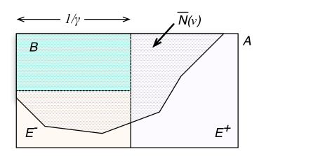
Figure 1: Illustration of the sets ${\overline{N}}(\nu)$, $A$, $B$, $E^{-}$ and $E^{+}$ in the proof of Lemma 13. Let $X\Subset Y$ mean that the facility sets $X$ is obtained from $Y$ by splitting facilities. We then have $A\Subset{\widetilde{N}}(j)$, $B\Subset{\widetilde{N}}_{{\mbox{\scriptsize\rm cls}}}(j)\cap{\overline{N}}_{{\mbox{\scriptsize\rm cls}}}(\kappa)$, $E^{-}\Subset{\widetilde{N}}_{{\mbox{\scriptsize\rm cls}}}(j)-{\overline{N}}_{{\mbox{\scriptsize\rm cls}}}(\kappa)$, $E^{+}\Subset{\widetilde{N}}(j)-{\widetilde{N}}_{{\mbox{\scriptsize\rm cls}}}(j)$.

We define the sets $A$, $B$, $E^{-}$ and $E^{+}$ as the subsets of $\overline{\mathbb{F}}$ (the final set of facilities) that were obtained from splitting facilities in the sets ${\widetilde{N}}(j)$, ${\widetilde{N}}_{{\mbox{\scriptsize\rm cls}}}(j)\cap{\overline{N}}_{{\mbox{\scriptsize\rm cls}}}(\kappa)$, ${\widetilde{N}}_{{\mbox{\scriptsize\rm cls}}}(j)-{\overline{N}}_{{\mbox{\scriptsize\rm cls}}}(\kappa)$ and ${\widetilde{N}}(j)-{\widetilde{N}}_{{\mbox{\scriptsize\rm cls}}}(j)$, respectively. (See Figure 1.) We claim that at the end $B\subseteq{\overline{N}}_{{\mbox{\scriptsize\rm cls}}}(\nu)$, with the caveat that the ties in the definition of ${\overline{N}}_{{\mbox{\scriptsize\rm cls}}}(\nu)$ are broken in favor of the facilities in $B$. (This is the tie-breaking rule that we mentioned in the definition of ${\overline{N}}_{{\mbox{\scriptsize\rm cls}}}(\nu)$.) This will be sufficient to prove the lemma because $B\neq\emptyset$, by the algorithm.

We now prove this claim. In this paragraph ${\overline{N}}(\nu)$ denotes the final set ${\overline{N}}(\nu)$ after both phases are completed. Thus the total connection value of ${\overline{N}}(\nu)$ to $\nu$ is $1$. Note first that $B\subseteq{\overline{N}}(\nu)\subseteq A$, because we never remove facilities from ${\overline{N}}(\nu)$ and we only add facilities from ${\widetilde{N}}(j)$. Also, $B\cup E^{-}$ represents the facilities obtained from ${\widetilde{N}}_{{\mbox{\scriptsize\rm cls}}}(j)$, so $\sum_{\mu\in B\cup E^{-}}{\bar{y}}_{\mu}=1/\gamma$. This and $B\subseteq{\overline{N}}(\nu)$ implies that the total connection value of $B\cup({\overline{N}}(\nu)\cap E^{-})$ to $\nu$ is at most $1/\gamma$. But all facilities in $B\cup({\overline{N}}(\nu)\cap E^{-})$ are closer to $\nu$ (taking into account our tie breaking in property (NB)) than those in $E^{+}\cap{\overline{N}}(\nu)$. It follows that $B\subseteq{\overline{N}}_{{\mbox{\scriptsize\rm cls}}}(\nu)$, completing the proof. ∎

Lemma 14.

Property (PD’.3(b)) holds.

Proof.

This proof is similar to that for Lemma 5. For a client $j$ and demand $\eta$, we will write $\mbox{\rm{tcc}}_{{\mbox{\scriptsize\rm cls}}}^{\eta}(j)$ and $\mbox{\rm{dmax}}_{{\mbox{\scriptsize\rm cls}}}^{\eta}(j)$ to denote the values of $\mbox{\rm{tcc}}_{{\mbox{\scriptsize\rm cls}}}(j)$ and $\mbox{\rm{dmax}}_{{\mbox{\scriptsize\rm cls}}}(j)$ at the time when $\eta$ was created. (Here $\eta$ may or may not be a demand of client $j$).

Suppose $\nu\in j$ is assigned to a primary demand $\kappa\in p$. By the way primary demands are constructed in the partitioning algorithm, ${\widetilde{N}}_{{\mbox{\scriptsize\rm cls}}}(p)$ becomes ${\overline{N}}(\kappa)$, which is equal to the final value of ${\overline{N}}_{{\mbox{\scriptsize\rm cls}}}(\kappa)$. So we have $C_{{\mbox{\scriptsize\rm cls}}}^{{\mbox{\scriptsize\rm avg}}}(\kappa)=\mbox{\rm{tcc}}_{{\mbox{\scriptsize\rm cls}}}^{\kappa}(p)$ and $C_{{\mbox{\scriptsize\rm cls}}}^{\max}(\kappa)=\mbox{\rm{dmax}}_{{\mbox{\scriptsize\rm cls}}}^{\kappa}(p)$. Further, since we choose $p$ to minimize $\mbox{\rm{tcc}}_{{\mbox{\scriptsize\rm cls}}}(p)+\mbox{\rm{dmax}}_{{\mbox{\scriptsize\rm cls}}}(p)$, we have that $\mbox{\rm{tcc}}_{{\mbox{\scriptsize\rm cls}}}^{\kappa}(p)+\mbox{\rm{dmax}}_{{\mbox{\scriptsize\rm cls}}}^{\kappa}(p)\leq\mbox{\rm{tcc}}_{{\mbox{\scriptsize\rm cls}}}^{\kappa}(j)+\mbox{\rm{dmax}}_{{\mbox{\scriptsize\rm cls}}}^{\kappa}(j)$.

Using an argument analogous to that in the proof of Lemma 4, our modified partitioning algorithm guarantees that $\mbox{\rm{tcc}}_{{\mbox{\scriptsize\rm cls}}}^{\kappa}(j)\leq\mbox{\rm{tcc}}_{{\mbox{\scriptsize\rm cls}}}^{\nu}(j)\leq C_{{\mbox{\scriptsize\rm cls}}}^{{\mbox{\scriptsize\rm avg}}}(\nu)$ and $\mbox{\rm{dmax}}_{{\mbox{\scriptsize\rm cls}}}^{\kappa}(j)\leq\mbox{\rm{dmax}}_{{\mbox{\scriptsize\rm cls}}}^{\nu}(j)\leq C_{{\mbox{\scriptsize\rm cls}}}^{\max}(\nu)$ since $\nu$ was created later. Therefore, we have

$$C_{{\mbox{\scriptsize\rm cls}}}^{{\mbox{\scriptsize\rm avg}}}(\kappa)+C_{{\mbox{\scriptsize\rm cls}}}^{\max}(\kappa) =\mbox{\rm{tcc}}_{{\mbox{\scriptsize\rm cls}}}^{\kappa}(p)+\mbox{\rm{dmax}}_{{\mbox{\scriptsize\rm cls}}}^{\kappa}(p)$$

$$\leq\mbox{\rm{tcc}}_{{\mbox{\scriptsize\rm cls}}}^{\kappa}(j)+\mbox{\rm{dmax}}_{{\mbox{\scriptsize\rm cls}}}^{\kappa}(j)\leq\mbox{\rm{tcc}}_{{\mbox{\scriptsize\rm cls}}}^{\nu}(j)+\mbox{\rm{dmax}}_{{\mbox{\scriptsize\rm cls}}}^{\nu}(j)\leq C_{{\mbox{\scriptsize\rm cls}}}^{{\mbox{\scriptsize\rm avg}}}(\nu)+C_{{\mbox{\scriptsize\rm cls}}}^{\max}(\nu),$$

completing the proof. ∎

Now we have completed the proof that the computed partitioning satisfies all the required properties.

Algorithm EBGS.

The complete algorithm starts with solving the LP(1) and computing the partitioning described earlier in this section. Given the partitioned fractional solution $(\bar{\boldsymbol{x}},\bar{\boldsymbol{y}})$ with the desired properties, we start the process of opening facilities and making connections to obtain an integral solution. To this end, for each primary demand $\kappa\in P$, we open exactly one facility $\phi(\kappa)$ in ${\overline{N}}_{{\mbox{\scriptsize\rm cls}}}(\kappa)$, where each $\mu\in{\overline{N}}_{{\mbox{\scriptsize\rm cls}}}(\kappa)$ is chosen as $\phi(\kappa)$ with probability $\gamma{\bar{y}}_{\mu}$. For all facilities $\mu\in\overline{\mathbb{F}}-\bigcup_{\kappa\in P}{\overline{N}}_{{\mbox{\scriptsize\rm cls}}}(\kappa)$, we open them independently, each with probability $\gamma{\bar{y}}_{\mu}$.

We claim that all probabilities are well-defined, that is $\gamma{\bar{y}}_{\mu}\leq 1$ for all $\mu$. Indeed, if ${\bar{y}}_{\mu}>0$ then ${\bar{y}}_{\mu}={\bar{x}}_{\mu\nu}$ for some $\nu$, by Property (CO). If $\mu\in{\overline{N}}_{{\mbox{\scriptsize\rm cls}}}(\nu)$ then the definition of close neighborhoods implies that ${\bar{x}}_{\mu\nu}\leq 1/\gamma$. If $\mu\in{\overline{N}}_{{\mbox{\scriptsize\rm far}}}(\nu)$ then ${\bar{x}}_{\mu\nu}\leq 1-1/\gamma\leq 1/\gamma$, because $\gamma<2$. Thus $\gamma{\bar{y}}_{\mu}\leq 1$, as claimed.

Next, we connect demands to facilities. Each primary demand $\kappa\in P$ will connect to the only open facility $\phi(\kappa)$ in ${\overline{N}}_{{\mbox{\scriptsize\rm cls}}}(\kappa)$. For each non-primary demand $\nu\in\overline{\mathbb{C}}-P$, if there is an open facility in ${\overline{N}}_{{\mbox{\scriptsize\rm cls}}}(\nu)$ then we connect $\nu$ to the nearest such facility. Otherwise, we connect $\nu$ to the nearest far facility in ${\overline{N}}_{{\mbox{\scriptsize\rm far}}}(\nu)$ if one is open. Otherwise, we connect $\nu$ to its target facility $\phi(\kappa)$, where $\kappa$ is the primary demand that $\nu$ is assigned to.

Analysis.

By the algorithm, for each client $j$, all its $r_{j}$ demands are connected to open facilities. If two different siblings $\nu,\nu^{\prime}\in j$ are assigned, respectively, to primary demands $\kappa$, $\kappa^{\prime}$ then, by Properties (SI’.1), (SI’.2), and (PD’.1) we have

$$({\overline{N}}(\nu)\cup{\overline{N}}_{{\mbox{\scriptsize\rm cls}}}(\kappa))\cap({\overline{N}}(\nu^{\prime})\cup{\overline{N}}_{{\mbox{\scriptsize\rm cls}}}(\kappa^{\prime}))=\emptyset.$$

This condition guarantees that $\nu$ and $\nu^{\prime}$ are assigned to different facilities, regardless whether they are connected to a neighbor facility or to its target facility. Therefore the computed solution is feasible.

We now estimate the cost of the solution computed by Algorithm EBGS. The lemma below bounds the expected facility cost.

Lemma 15.

The expectation of facility cost $F_{\mbox{\tiny\rm EBGS}}$ of Algorithm EBGS is at most $\gamma F^{\ast}$.

Proof.

By the algorithm, each facility $\mu\in\overline{\mathbb{F}}$ is opened with probability $\gamma{\bar{y}}_{\mu}$, independently of whether it belongs to the close neighborhood of a primary demand or not. Therefore, by linearity of expectation, we have that the expected facility cost is

$$\mathbb{E}[F_{\mbox{\tiny\rm EBGS}}]=\sum_{\mu\in\overline{\mathbb{F}}}f_{\mu}\gamma{\bar{y}}_{\mu}=\gamma\sum_{i\in\mathbb{F}}f_{i}\sum_{\mu\in i}{\bar{y}}_{\mu}=\gamma\sum_{i\in\mathbb{F}}f_{i}y_{i}^{\ast}=\gamma F^{\ast},$$

where the third equality follows from (PS.3). ∎

In the remainder of this section we focus on the connection cost. Let $C_{\nu}$ be the random variable representing the connection cost of a demand $\nu$. Our objective is to show that the expectation of $\nu$ satisfies

$$\mathbb{E}[C_{\nu}]\leq C^{{\mbox{\scriptsize\rm avg}}}(\nu)\cdot\max\left\{\frac{1/e+1/e^{\gamma}}{1-1/\gamma},1+\frac{2}{e^{\gamma}}\right\}.$$ (11)

If $\nu$ is a primary demand then, due to the algorithm, we have $\mathbb{E}[C_{\nu}]=C_{{\mbox{\scriptsize\rm cls}}}^{{\mbox{\scriptsize\rm avg}}}(\nu)\leq C^{{\mbox{\scriptsize\rm avg}}}(\nu)$, so (11) is easily satisfied.

Thus for the rest of the argument we will focus on the case when $\nu$ is a non-primary demand. Recall that the algorithm connects $\nu$ to the nearest open facility in ${\overline{N}}_{{\mbox{\scriptsize\rm cls}}}(\nu)$ if at least one facility in ${\overline{N}}_{{\mbox{\scriptsize\rm cls}}}(\nu)$ is open. Otherwise the algorithm connects $\nu$ to the nearest open facility in ${\overline{N}}_{{\mbox{\scriptsize\rm far}}}(\nu)$, if any. In the event that no facility in ${\overline{N}}(\nu)$ opens, the algorithm will connect $\nu$ to its target facility $\phi(\kappa)$, where $\kappa$ is the primary demand that $\nu$ was assigned to, and $\phi(\kappa)$ is the only facility open in ${\overline{N}}_{{\mbox{\scriptsize\rm cls}}}(\kappa)$. Let $\Lambda^{\nu}$ denote the event that at least one facility in ${\overline{N}}(\nu)$ is open and $\Lambda^{\nu}_{{\mbox{\scriptsize\rm cls}}}$ be the event that at least one facility in ${\overline{N}}_{{\mbox{\scriptsize\rm cls}}}(\nu)$ is open. $\neg\Lambda^{\nu}$ denotes the complement event of $\Lambda^{\nu}$, that is, the event that none of $\nu$’s neighbors opens. We want to estimate the following three conditional expectations:

$$\mathbb{E}[C_{\nu}\mid\Lambda^{\nu}_{{\mbox{\scriptsize\rm cls}}}],\quad\mathbb{E}[C_{\nu}\mid\Lambda^{\nu}\wedge\neg\Lambda^{\nu}_{{\mbox{\scriptsize\rm cls}}}],\quad\text{and}\quad\mathbb{E}[C_{\nu}\mid\neg\Lambda^{\nu}],$$

and their associated probabilities.

We start with a lemma dealing with the third expectation, $\mathbb{E}[C_{\nu}\mid\neg\Lambda^{\nu}]=\mathbb{E}[d_{\phi(\kappa)\nu}\mid\Lambda^{\nu}]$. The proof of this lemma relies on Properties (PD’.3(a)) and (PD’.3(b)) of modified partitioning and follows the reasoning in the proof of a similar lemma in [3, 2]. For the sake of completeness, we include a proof in A.

Lemma 16.

Assuming that no facility in ${\overline{N}}(\nu)$ opens, the expected connection cost of $\nu$ is

$$\mathbb{E}[C_{\nu}\mid\neg\Lambda^{\nu}]\leq C_{{\mbox{\scriptsize\rm cls}}}^{{\mbox{\scriptsize\rm avg}}}(\nu)+2C_{{\mbox{\scriptsize\rm far}}}^{{\mbox{\scriptsize\rm avg}}}(\nu).$$ (12)

Proof.

See A. ∎

Next, we derive some estimates for the expected cost of direct connections. The next technical lemma is a generalization of Lemma 10. In Lemma 10 we bound the expected distance to the closest open facility in ${\overline{N}}(\nu)$, conditioned on at least one facility in ${\overline{N}}(\nu)$ being open. The lemma below provides a similar estimate for an arbitrary set $A$ of facilities in ${\overline{N}}(\nu)$, conditioned on that at least one facility in set $A$ is open. Recall that $D(A,\nu)=\sum_{\mu\in A}d_{\mu\nu}{\bar{y}}_{\mu}/\sum_{\mu\in A}{\bar{y}}_{\mu}$ is the average distance from $\nu$ to a facility in $A$.

Lemma 17.

For any non-empty set $A\subseteq{\overline{N}}(\nu)$, let $\Lambda^{\nu}_{A}$ be the event that at least one facility in $A$ is opened by Algorithm EBGS, and denote by $C_{\nu}(A)$ the random variable representing the distance from $\nu$ to the closest open facility in $A$. Then the expected distance from $\nu$ to the nearest open facility in $A$, conditioned on at least one facility in $A$ being opened, is

$$\mathbb{E}[C_{\nu}(A)\mid\Lambda^{\nu}_{A}]\leq D(A,\nu).$$

Proof.

The proof follows the same reasoning as the proof of Lemma 10, so we only sketch it here. We start with a similar grouping of facilities in $A$: for each primary demand $\kappa$, if ${\overline{N}}_{{\mbox{\scriptsize\rm cls}}}(\kappa)\cap A\neq\emptyset$ then ${\overline{N}}_{{\mbox{\scriptsize\rm cls}}}(\kappa)\cap A$ forms a group. Facilities in $A$ that are not in a neighborhood of any primary demand form singleton groups. We denote these groups $G_{1},...,G_{k}$. It is clear that the groups are disjoint because of (PD’.1). Denoting by ${\bar{d}}_{s}=D(G_{s},\nu)$ the average distance from $\nu$ to a group $G_{s}$, we can assume that these groups are ordered so that ${\bar{d}}_{1}\leq...\leq{\bar{d}}_{k}$.

Each group can have at most one facility open and the events representing opening of any two facilities that belong to different groups are independent. To estimate the distance from $\nu$ to the nearest open facility in $A$, we use an alternative random process to make connections, that is easier to analyze. Instead of connecting $\nu$ to the nearest open facility in $A$, we will choose the smallest $s$ for which $G_{s}$ has an open facility and connect $\nu$ to this facility. (Thus we selected an open facility with respect to the minimum ${\bar{d}}_{s}$, not the actual distance from $\nu$ to this facility.) This can only increase the expected connection cost, thus denoting $g_{s}=\sum_{\mu\in G_{s}}\gamma{\bar{y}}_{\mu}$ for all $s=1,\ldots,k$, and letting $\mathbb{P}[\Lambda^{\nu}_{A}]$ be the probability that $A$ has at least one facility open, we have

$$\mathbb{E}[C_{\nu}(A)\mid\Lambda^{\nu}_{A}] \leq\frac{1}{\mathbb{P}[\Lambda^{\nu}_{A}]}({\bar{d}}_{1}g_{1}+{\bar{d}}_{2}g_{2}(1-g_{1})+\ldots+{\bar{d}}_{k}g_{k}(1-g_{1})\ldots(1-g_{k-1}))$$ (13)

$$\leq\frac{1}{\mathbb{P}[\Lambda^{\nu}_{A}]}\frac{\sum_{s=1}^{k}{\bar{d}}_{s}g_{s}}{\sum_{s=1}^{k}g_{s}}(1-\prod_{s=1}^{k}(1-g_{s}))$$ (14)

$$=\frac{\sum_{s=1}^{k}{\bar{d}}_{s}g_{s}}{\sum_{s=1}^{k}g_{s}}=\frac{\sum_{\mu\in A}d_{\mu\nu}\gamma{\bar{y}}_{\mu}}{\sum_{\mu\in A}\gamma{\bar{y}}_{\mu}}$$

$$=\frac{\sum_{s=1}^{k}d_{\mu\nu}{\bar{y}}_{\mu}}{\sum_{\mu\in A}{\bar{y}}_{\mu}}=D(A,\nu).$$

Inequality (14) follows from inequality (22) in B. The rest of the derivation follows from $\mathbb{P}[\Lambda^{\nu}_{A}]=1-\prod_{s=1}^{k}(1-g_{s})$, and the definition of ${\bar{d}}_{s}$, $g_{s}$ and $D(A,\nu)$. ∎

A consequence of Lemma 17 is the following corollary which bounds the other two expectations of $C_{\nu}$, when at least one facility is opened in ${\overline{N}}_{{\mbox{\scriptsize\rm cls}}}(\nu)$, and when no facility in ${\overline{N}}_{{\mbox{\scriptsize\rm cls}}}(\nu)$ opens but a facility in ${\overline{N}}_{{\mbox{\scriptsize\rm far}}}(\nu)$ is opened.

Corollary 18.

(a) $\mathbb{E}[C_{\nu}\mid\Lambda_{{\mbox{\scriptsize\rm cls}}}^{\nu}]\leq C_{{\mbox{\scriptsize\rm cls}}}^{{\mbox{\scriptsize\rm avg}}}(\nu)$, and (b) $\mathbb{E}[C_{\nu}\mid\Lambda^{\nu}\wedge\neg\Lambda_{{\mbox{\scriptsize\rm cls}}}^{\nu}]\leq C_{{\mbox{\scriptsize\rm far}}}^{{\mbox{\scriptsize\rm avg}}}(\nu)$.

Proof.

When there is an open facility in ${\overline{N}}_{{\mbox{\scriptsize\rm cls}}}(\nu)$, the algorithm connect $\nu$ to the nearest open facility in ${\overline{N}}_{{\mbox{\scriptsize\rm cls}}}(\nu)$. When no facility in ${\overline{N}}_{{\mbox{\scriptsize\rm cls}}}(\nu)$ opens but some facility in ${\overline{N}}_{{\mbox{\scriptsize\rm far}}}(\nu)$ opens, the algorithm connects $\nu$ to the nearest open facility in ${\overline{N}}_{{\mbox{\scriptsize\rm far}}}(\nu)$. The rest of the proof follows from Lemma 17. By setting the set $A$ in Lemma 17 to ${\overline{N}}_{{\mbox{\scriptsize\rm cls}}}(\nu)$, we have

$$\mathbb{E}[C_{\nu}\mid\Lambda_{{\mbox{\scriptsize\rm cls}}}^{\nu}]\leq D({\overline{N}}_{{\mbox{\scriptsize\rm cls}}}(\nu),\nu),=C_{{\mbox{\scriptsize\rm cls}}}^{{\mbox{\scriptsize\rm avg}}}(\nu),$$

proving part (a), and by setting the set $A$ to ${\overline{N}}_{{\mbox{\scriptsize\rm far}}}(\nu)$, we have

$$\mathbb{E}[C_{\nu}\mid\Lambda^{\nu}\wedge\neg\Lambda_{{\mbox{\scriptsize\rm cls}}}^{\nu}]\leq D({\overline{N}}_{{\mbox{\scriptsize\rm far}}}(\nu),\nu)=C_{{\mbox{\scriptsize\rm far}}}^{{\mbox{\scriptsize\rm avg}}}(\nu),$$

which proves part (b). ∎

Given the estimate on the three expected distances when $\nu$ connects to its close facility in ${\overline{N}}_{{\mbox{\scriptsize\rm cls}}}(\nu)$ in (7), or its far facility in ${\overline{N}}_{{\mbox{\scriptsize\rm far}}}(\nu)$ in (7), or its target facility $\phi(\kappa)$ in (12), the only missing pieces are estimates on the corresponding probabilities of each event, which we do in the next lemma. Once done, we shall put all pieces together and proving the desired inequality on $\mathbb{E}[C_{\nu}]$, that is (11).

The next Lemma bounds the probabilities for events that no facilities in ${\overline{N}}_{{\mbox{\scriptsize\rm cls}}}(\nu)$ and ${\overline{N}}(\nu)$ are opened by the algorithm.

Lemma 19.

(a) $\mathbb{P}[\neg\Lambda^{\nu}_{{\mbox{\scriptsize\rm cls}}}]\leq 1/e$, and (b) $\mathbb{P}[\neg\Lambda^{\nu}]\leq 1/e^{\gamma}$.

Proof.

(a) To estimate $\mathbb{P}[\neg\Lambda^{\nu}_{{\mbox{\scriptsize\rm cls}}}]$, we again consider a grouping of facilities in ${\overline{N}}_{{\mbox{\scriptsize\rm cls}}}(\nu)$, as in the proof of Lemma 17, according to the primary demand’s close neighborhood that they fall in, with facilities not belonging to such neighborhoods forming their own singleton groups. As before, the groups are denoted $G_{1},\ldots,G_{k}$. It is easy to see that $\sum_{s=1}^{k}g_{s}=\sum_{\mu\in{\overline{N}}_{{\mbox{\scriptsize\rm cls}}}(\nu)}\gamma{\bar{y}}_{\mu}=1$. For any group $G_{s}$, the probability that a facility in this group opens is $\sum_{\mu\in G_{s}}\gamma{\bar{y}}_{\mu}=g_{s}$ because in the algorithm at most one facility in a group can be chosen and each is chosen with probability $\gamma{\bar{y}}_{\mu}$. Therefore the probability that no facility opens is $\prod_{s=1}^{k}(1-g_{s})$, which is at most $e^{-\sum_{s=1}^{k}g_{s}}=1/e$. Therefore we have $\mathbb{P}[\neg\Lambda^{\nu}_{A}]\leq 1/e$.

(b) This proof is similar to the proof of (a). The probability $\mathbb{P}[\neg\Lambda^{\nu}]$ is at most $e^{-\sum_{s=1}^{k}g_{s}}=1/e^{\gamma}$, because we now have $\sum_{s=1}^{k}g_{s}=\gamma\sum_{\mu\in{\overline{N}}(\nu)}{\bar{y}}_{\mu}=\gamma\cdot 1=\gamma$. ∎

We are now ready to bound the overall connection cost of Algorithm EBGS, namely inequality (11).

Lemma 20.

The expected connection of $\nu$ is

$$\mathbb{E}[C_{\nu}]\leq C^{{\mbox{\scriptsize\rm avg}}}(\nu)\cdot\max\Big{\{}\frac{1/e+1/e^{\gamma}}{1-1/\gamma},1+\frac{2}{e^{\gamma}}\Big{\}}.$$

Proof.

Recall that, to connect $\nu$, the algorithm uses the closest facility in ${\overline{N}}_{{\mbox{\scriptsize\rm cls}}}(\nu)$ if one is opened; otherwise it will try to connect $\nu$ to the closest facility in ${\overline{N}}_{{\mbox{\scriptsize\rm far}}}(\nu)$. Failing that, it will connect $\nu$ to $\phi(\kappa)$, the sole facility open in the neighborhood of $\kappa$, the primary demand $\nu$ was assigned to. Given that, we estimate $\mathbb{E}[C_{\nu}]$ as follows:

$$\mathbb{E}[C_{\nu}]\; =\;\mathbb{E}[C_{\nu}\mid\Lambda^{\nu}_{{\mbox{\scriptsize\rm cls}}}]\cdot\mathbb{P}[\Lambda^{\nu}_{{\mbox{\scriptsize\rm cls}}}]\;+\;\mathbb{E}[C_{\nu}\mid\Lambda^{\nu}\ \wedge\neg\Lambda^{\nu}_{{\mbox{\scriptsize\rm cls}}}]\cdot\mathbb{P}[\Lambda^{\nu}\,\wedge\neg\Lambda^{\nu}_{{\mbox{\scriptsize\rm cls}}}]$$

$$\quad\quad\quad+\;\mathbb{E}[C_{\nu}\mid\neg\Lambda^{\nu}]\cdot\mathbb{P}[\neg\Lambda^{\nu}]$$

$$\leq\;C_{{\mbox{\scriptsize\rm cls}}}^{{\mbox{\scriptsize\rm avg}}}(\nu)\cdot\mathbb{P}[\Lambda^{\nu}_{{\mbox{\scriptsize\rm cls}}}]\;+\;C_{{\mbox{\scriptsize\rm far}}}^{{\mbox{\scriptsize\rm avg}}}(\nu)\cdot\mathbb{P}[\Lambda^{\nu}\,\wedge\neg\Lambda^{\nu}_{{\mbox{\scriptsize\rm cls}}}]$$ (15)

$$\quad\quad\quad+\;[\,C_{{\mbox{\scriptsize\rm cls}}}^{{\mbox{\scriptsize\rm avg}}}(\nu)+2C_{{\mbox{\scriptsize\rm far}}}^{{\mbox{\scriptsize\rm avg}}}(\nu)\,]\cdot\mathbb{P}[\neg\Lambda^{\nu}]$$

$$=\;[\,C_{{\mbox{\scriptsize\rm cls}}}^{{\mbox{\scriptsize\rm avg}}}(\nu)+C_{{\mbox{\scriptsize\rm far}}}^{{\mbox{\scriptsize\rm avg}}}(\nu)\,]\cdot\mathbb{P}[\neg\Lambda^{\nu}]\;+\;[\,C_{{\mbox{\scriptsize\rm far}}}^{{\mbox{\scriptsize\rm avg}}}(\nu)-C_{{\mbox{\scriptsize\rm cls}}}^{{\mbox{\scriptsize\rm avg}}}(\nu)\,]\cdot\mathbb{P}[\neg\Lambda^{\nu}_{{\mbox{\scriptsize\rm cls}}}]\;+\;C_{{\mbox{\scriptsize\rm cls}}}^{{\mbox{\scriptsize\rm avg}}}(\nu)$$

$$\leq\;[\,C_{{\mbox{\scriptsize\rm cls}}}^{{\mbox{\scriptsize\rm avg}}}(\nu)+C_{{\mbox{\scriptsize\rm far}}}^{{\mbox{\scriptsize\rm avg}}}(\nu)\,]\cdot\frac{1}{e^{\gamma}}\;+\;[\,C_{{\mbox{\scriptsize\rm far}}}^{{\mbox{\scriptsize\rm avg}}}(\nu)-C_{{\mbox{\scriptsize\rm cls}}}^{{\mbox{\scriptsize\rm avg}}}(\nu)\,]\cdot\frac{1}{e}\;+\;C_{{\mbox{\scriptsize\rm cls}}}^{{\mbox{\scriptsize\rm avg}}}(\nu)$$ (16)

$$=\;\Big{(}1-\frac{1}{e}+\frac{1}{e^{\gamma}}\Big{)}\cdot C_{{\mbox{\scriptsize\rm cls}}}^{{\mbox{\scriptsize\rm avg}}}(\nu)\;+\;\Big{(}\frac{1}{e}+\frac{1}{e^{\gamma}}\Big{)}\cdot C_{{\mbox{\scriptsize\rm far}}}^{{\mbox{\scriptsize\rm avg}}}(\nu).$$

Inequality (15) follows from Corollary 18 and Lemma 16. Inequality (16) follows from Lemma 19 and $C_{{\mbox{\scriptsize\rm far}}}^{{\mbox{\scriptsize\rm avg}}}(\nu)-C_{{\mbox{\scriptsize\rm cls}}}^{{\mbox{\scriptsize\rm avg}}}(\nu)\geq 0$.

Now define $\rho=C_{{\mbox{\scriptsize\rm cls}}}^{{\mbox{\scriptsize\rm avg}}}(\nu)/C^{{\mbox{\scriptsize\rm avg}}}(\nu)$. It is easy to see that $\rho$ is between 0 and 1. Continuing the above derivation, applying (10), we get

$$\mathbb{E}[C_{\nu}]\; \leq\;C^{{\mbox{\scriptsize\rm avg}}}(\nu)\cdot\left((1-\rho)\frac{1/e+1/e^{\gamma}}{1-1/\gamma}+\rho(1+\frac{2}{e^{\gamma}})\right)$$

$$\leq C^{{\mbox{\scriptsize\rm avg}}}(\nu)\cdot\max\left\{\frac{1/e+1/e^{\gamma}}{1-1/\gamma},1+\frac{2}{e^{\gamma}}\right\},$$

and the proof is now complete. ∎

With Lemma 20 proven, we are now ready to bound our total connection cost. For any client $j$ we have

$$\sum_{\nu\in j}C^{{\mbox{\scriptsize\rm avg}}}(\nu) =\sum_{\nu\in j}\sum_{\mu\in\overline{\mathbb{F}}}d_{\mu\nu}{\bar{x}}_{\mu\nu}$$

$$=\sum_{i\in\mathbb{F}}d_{ij}\sum_{\mu\in i}\sum_{\nu\in j}{\bar{x}}_{\mu\nu}=\sum_{i\in\mathbb{F}}d_{ij}x_{ij}^{\ast}=C_{j}^{\ast}.$$

Summing over all clients $j$ we obtain that the total expected connection cost is

$$\mathbb{E}[C_{\mbox{\tiny\rm EBGS}}]\leq C^{\ast}\max\left\{\frac{1/e+1/e^{\gamma}}{1-1/\gamma},1+\frac{2}{e^{\gamma}}\right\}.$$

Recall that the expected facility cost is bounded by $\gamma F^{\ast}$, as argued earlier. Hence the total expected cost is bounded by $\max\{\gamma,\frac{1/e+1/e^{\gamma}}{1-1/\gamma},1+\frac{2}{e^{\gamma}}\}\cdot\mbox{\rm LP}^{\ast}$. Picking $\gamma=1.575$ we obtain the desired ratio.

Theorem 21.

Algorithm EBGS is a $1.575$-approximation algorithm for FTFP.

8 Final Comments

In this paper we show a sequence of LP-rounding approximation algorithms for FTFP, with the best algorithm achieving ratio $1.575$. As we mentioned earlier, we believe that our techniques of demand reduction and adaptive partitioning are very flexible and should be useful in extending other LP-rounding methods for UFL to obtain matching bounds for FTFP.

One of the main open problems in this area is whether FTFL can be approximated with the same ratio as UFL, and our work was partly motivated by this question. The techniques we introduced are not directly applicable to FTFL, mainly because our partitioning approach involves facility splitting that could result in several sibling demands being served by facilities on the same site. Nonetheless, we hope that further refinements of our construction might get around this issue and lead to new algorithms for FTFL with improved ratios.

Appendix A Proof of Lemma 16

Lemma 16 provides a bound on the expected connection cost of a demand $\nu$ when Algorithm EBGS does not open any facilities in ${\overline{N}}(\nu)$, namely

$$\mathbb{E}[C_{\nu}\mid\neg\Lambda^{\nu}]\leq C_{{\mbox{\scriptsize\rm cls}}}^{{\mbox{\scriptsize\rm avg}}}(\nu)+2C_{{\mbox{\scriptsize\rm far}}}^{{\mbox{\scriptsize\rm avg}}}(\nu),$$ (17)

We show a stronger inequality that

$$\mathbb{E}[C_{\nu}\mid\neg\Lambda^{\nu}]\leq C_{{\mbox{\scriptsize\rm cls}}}^{{\mbox{\scriptsize\rm avg}}}(\nu)+C_{{\mbox{\scriptsize\rm cls}}}^{\max}(\nu)+C_{{\mbox{\scriptsize\rm far}}}^{{\mbox{\scriptsize\rm avg}}}(\nu),$$ (18)

which then implies (17) because $C_{{\mbox{\scriptsize\rm cls}}}^{\max}(\nu)\leq C_{{\mbox{\scriptsize\rm far}}}^{{\mbox{\scriptsize\rm avg}}}(\nu)$. The proof of (18) is similar to that in [2]. For the sake of completeness, we provide it here, formulated in our terminology and notation.

Assume that the event $\neg\Lambda^{\nu}$ is true, that is Algorithm EBGS does not open any facility in ${\overline{N}}(\nu)$. Let $\kappa$ be the primary demand that $\nu$ was assigned to. Also let

$$K={\overline{N}}_{{\mbox{\scriptsize\rm cls}}}(\kappa)\setminus{\overline{N}}(\nu),\quad V_{{\mbox{\scriptsize\rm cls}}}={\overline{N}}_{{\mbox{\scriptsize\rm cls}}}(\kappa)\cap{\overline{N}}_{{\mbox{\scriptsize\rm cls}}}(\nu)\quad\textrm{and}\quad V_{{\mbox{\scriptsize\rm far}}}={\overline{N}}_{{\mbox{\scriptsize\rm cls}}}(\kappa)\cap{\overline{N}}_{{\mbox{\scriptsize\rm far}}}(\nu).$$

Then $K,V_{{\mbox{\scriptsize\rm cls}}},V_{{\mbox{\scriptsize\rm far}}}$ form a partition of ${\overline{N}}_{{\mbox{\scriptsize\rm cls}}}(\kappa)$, that is, they are disjoint and their union is ${\overline{N}}_{{\mbox{\scriptsize\rm cls}}}(\kappa)$. Moreover, we have that $K$ is not empty, because Algorithm EBGS opens some facility in ${\overline{N}}_{{\mbox{\scriptsize\rm cls}}}(\kappa)$ and this facility cannot be in $V_{{\mbox{\scriptsize\rm cls}}}\cup V_{{\mbox{\scriptsize\rm far}}}$, by our assumption. We also have that $V_{{\mbox{\scriptsize\rm cls}}}$ is not empty due to (PD’.3(a)).

Recall that $D(A,\eta)=\sum_{\mu\in A}d_{\mu\eta}{\bar{y}}_{\mu}/\sum_{\mu\in A}{\bar{y}}_{\mu}$ is the average distance between a demand $\eta$ and the facilities in a set $A$. We shall show that

$$D(K,\nu)\leq C_{{\mbox{\scriptsize\rm cls}}}^{{\mbox{\scriptsize\rm avg}}}(\kappa)+C_{{\mbox{\scriptsize\rm cls}}}^{\max}(\kappa)+C_{{\mbox{\scriptsize\rm far}}}^{{\mbox{\scriptsize\rm avg}}}(\nu).$$ (19)

This is sufficient, because, by the algorithm, $D(K,\nu)$ is exactly the expected connection cost for demand $\nu$ conditioned on the event that none of $\nu$’s neighbors opens, that is the left-hand side of (18). Further, (PD’.3(b)) states that $C_{{\mbox{\scriptsize\rm cls}}}^{{\mbox{\scriptsize\rm avg}}}(\kappa)+C_{{\mbox{\scriptsize\rm cls}}}^{\max}(\kappa)\leq C_{{\mbox{\scriptsize\rm cls}}}^{{\mbox{\scriptsize\rm avg}}}(\nu)+C_{{\mbox{\scriptsize\rm cls}}}^{\max}(\nu)$, and thus (19) implies (18).

The proof of (19) is by analysis of several cases.

Case 1: $D(K,\kappa)\leq C_{{\mbox{\scriptsize\rm cls}}}^{{\mbox{\scriptsize\rm avg}}}(\kappa)$. For any facility $\mu\in V_{{\mbox{\scriptsize\rm cls}}}$ (recall that $V_{{\mbox{\scriptsize\rm cls}}}\neq\emptyset$), we have $d_{\mu\kappa}\leq C_{{\mbox{\scriptsize\rm cls}}}^{\max}(\kappa)$ and $d_{\mu\nu}\leq C_{{\mbox{\scriptsize\rm cls}}}^{\max}(\nu)\leq C_{{\mbox{\scriptsize\rm far}}}^{{\mbox{\scriptsize\rm avg}}}(\nu)$. Therefore, using the case assumption, we get $D(K,\nu)\leq D(K,\kappa)+d_{\mu\kappa}+d_{\mu\nu}\leq C_{{\mbox{\scriptsize\rm cls}}}^{{\mbox{\scriptsize\rm avg}}}(\kappa)+C_{{\mbox{\scriptsize\rm cls}}}^{\max}(\kappa)+C_{{\mbox{\scriptsize\rm far}}}^{{\mbox{\scriptsize\rm avg}}}(\nu)$.

Case 2: There exists a facility $\mu\in V_{{\mbox{\scriptsize\rm cls}}}$ such that $d_{\mu\kappa}\leq C_{{\mbox{\scriptsize\rm cls}}}^{{\mbox{\scriptsize\rm avg}}}(\kappa)$. Since $\mu\in V_{{\mbox{\scriptsize\rm cls}}}$, we infer that $d_{\mu\nu}\leq C_{{\mbox{\scriptsize\rm cls}}}^{\max}(\nu)\leq C_{{\mbox{\scriptsize\rm far}}}^{{\mbox{\scriptsize\rm avg}}}(\nu)$. Using $C_{{\mbox{\scriptsize\rm cls}}}^{\max}(\kappa)$ to bound $D(K,\kappa)$, we have $D(K,\nu)\leq D(K,\kappa)+d_{\mu\kappa}+d_{\mu\nu}\leq C_{{\mbox{\scriptsize\rm cls}}}^{\max}(\kappa)+C_{{\mbox{\scriptsize\rm cls}}}^{{\mbox{\scriptsize\rm avg}}}(\kappa)+C_{{\mbox{\scriptsize\rm far}}}^{{\mbox{\scriptsize\rm avg}}}(\nu)$.

Case 3: In this case we assume that neither of Cases 1 and 2 applies, that is $D(K,\kappa)>C_{{\mbox{\scriptsize\rm cls}}}^{{\mbox{\scriptsize\rm avg}}}(\kappa)$ and every $\mu\in V_{{\mbox{\scriptsize\rm cls}}}$ satisfies $d_{\mu\kappa}>C_{{\mbox{\scriptsize\rm cls}}}^{{\mbox{\scriptsize\rm avg}}}(\kappa)$. This implies that $D(K\cup V_{{\mbox{\scriptsize\rm cls}}},\kappa)>C_{{\mbox{\scriptsize\rm cls}}}^{{\mbox{\scriptsize\rm avg}}}(\kappa)=D({\overline{N}}_{{\mbox{\scriptsize\rm cls}}}(\kappa),\kappa)$. Since sets $K$, $V_{{\mbox{\scriptsize\rm cls}}}$ and $V_{{\mbox{\scriptsize\rm far}}}$ form a partition of ${\overline{N}}_{{\mbox{\scriptsize\rm cls}}}(\kappa)$, we obtain that in this case $V_{{\mbox{\scriptsize\rm far}}}$ is not empty and $D(V_{{\mbox{\scriptsize\rm far}}},\kappa)<C_{{\mbox{\scriptsize\rm cls}}}^{{\mbox{\scriptsize\rm avg}}}(\kappa)$. Let $\delta=C_{{\mbox{\scriptsize\rm cls}}}^{{\mbox{\scriptsize\rm avg}}}(\kappa)-D(V_{{\mbox{\scriptsize\rm far}}},\kappa)>0$. We now have two sub-cases:

Case 3.1: $D(V_{{\mbox{\scriptsize\rm far}}},\nu)\leq C_{{\mbox{\scriptsize\rm far}}}^{{\mbox{\scriptsize\rm avg}}}(\nu)+\delta$. Substituting $\delta$, this implies that $D(V_{{\mbox{\scriptsize\rm far}}},\nu)+D(V_{{\mbox{\scriptsize\rm far}}},\kappa)\leq C_{{\mbox{\scriptsize\rm cls}}}^{{\mbox{\scriptsize\rm avg}}}(\kappa)+C_{{\mbox{\scriptsize\rm far}}}^{{\mbox{\scriptsize\rm avg}}}(\nu)$. From the definition of the average distance $D(V_{{\mbox{\scriptsize\rm far}}},\kappa)$ and $D(V_{{\mbox{\scriptsize\rm far}}},\nu)$, we obtain that there exists some $\mu\in V_{{\mbox{\scriptsize\rm far}}}$ such that $d_{\mu\kappa}+d_{\mu\nu}\leq C_{{\mbox{\scriptsize\rm cls}}}^{{\mbox{\scriptsize\rm avg}}}(\kappa)+C_{{\mbox{\scriptsize\rm far}}}^{{\mbox{\scriptsize\rm avg}}}(\nu)$. Thus $D(K,\nu)\leq D(K,\kappa)+d_{\mu\kappa}+d_{\mu\nu}\leq C_{{\mbox{\scriptsize\rm cls}}}^{\max}(\kappa)+C_{{\mbox{\scriptsize\rm cls}}}^{{\mbox{\scriptsize\rm avg}}}(\kappa)+C_{{\mbox{\scriptsize\rm far}}}^{{\mbox{\scriptsize\rm avg}}}(\nu)$.

Case 3.2: $D(V_{{\mbox{\scriptsize\rm far}}},\nu)>C_{{\mbox{\scriptsize\rm far}}}^{{\mbox{\scriptsize\rm avg}}}(\nu)+\delta$. The case assumption implies that $V_{{\mbox{\scriptsize\rm far}}}$ is a proper subset of ${\overline{N}}_{{\mbox{\scriptsize\rm far}}}(\nu)$, that is ${\overline{N}}_{{\mbox{\scriptsize\rm far}}}(\nu)\setminus V_{{\mbox{\scriptsize\rm far}}}\neq\emptyset$. Let $\hat{y}=\gamma\sum_{\mu\in V_{{\mbox{\tiny\rm far}}}}{\bar{y}}_{\mu}$. We can express $C_{{\mbox{\scriptsize\rm far}}}^{{\mbox{\scriptsize\rm avg}}}(\nu)$ using $\hat{y}$ as follows

$$C_{{\mbox{\scriptsize\rm far}}}^{{\mbox{\scriptsize\rm avg}}}(\nu)=D(V_{{\mbox{\scriptsize\rm far}}},\nu)\frac{\hat{y}}{\gamma-1}+D({\overline{N}}_{{\mbox{\scriptsize\rm far}}}(\nu)\setminus V_{{\mbox{\scriptsize\rm far}}},\nu)\frac{\gamma-1-\hat{y}}{\gamma-1}.$$

Then, using the case condition and simple algebra, we have

$$C_{{\mbox{\scriptsize\rm cls}}}^{\max}(\nu) \leq D({\overline{N}}_{{\mbox{\scriptsize\rm far}}}(\nu)\setminus V_{{\mbox{\scriptsize\rm far}}},\nu)$$

$$\leq C_{{\mbox{\scriptsize\rm far}}}^{{\mbox{\scriptsize\rm avg}}}(\nu)-\frac{\hat{y}\delta}{\gamma-1-\hat{y}}\leq C_{{\mbox{\scriptsize\rm far}}}^{{\mbox{\scriptsize\rm avg}}}(\nu)-\frac{\hat{y}\delta}{1-\hat{y}},$$ (20)

where the last step follows from $1<\gamma<2$.

On the other hand, since $K$, $V_{{\mbox{\scriptsize\rm cls}}}$, and $V_{{\mbox{\scriptsize\rm far}}}$ form a partition of ${\overline{N}}_{{\mbox{\scriptsize\rm cls}}}(\kappa)$, we have $C_{{\mbox{\scriptsize\rm cls}}}^{{\mbox{\scriptsize\rm avg}}}(\kappa)=(1-\hat{y})D(K\cup V_{{\mbox{\scriptsize\rm cls}}},\kappa)+\hat{y}D(V_{{\mbox{\scriptsize\rm far}}},\kappa)$. Then using the definition of $\delta$ we obtain

$$D(K\cup V_{{\mbox{\scriptsize\rm cls}}},\kappa)=C_{{\mbox{\scriptsize\rm cls}}}^{{\mbox{\scriptsize\rm avg}}}(\kappa)+\frac{\hat{y}\delta}{1-\hat{y}}.$$ (21)

Now we are essentially done. If there exists some $\mu\in V_{{\mbox{\scriptsize\rm cls}}}$ such that $d_{\mu\kappa}\leq C_{{\mbox{\scriptsize\rm cls}}}^{{\mbox{\scriptsize\rm avg}}}(\kappa)+\hat{y}\delta/(1-\hat{y})$, then we have

$$D(K,\nu) \leq D(K,\kappa)+d_{\mu\kappa}+d_{\mu\nu}$$

$$\leq C_{{\mbox{\scriptsize\rm cls}}}^{\max}(\kappa)+C_{{\mbox{\scriptsize\rm cls}}}^{{\mbox{\scriptsize\rm avg}}}(\kappa)+\frac{\hat{y}\delta}{1-\hat{y}}+C_{{\mbox{\scriptsize\rm cls}}}^{\max}(\nu)$$

$$\leq C_{{\mbox{\scriptsize\rm cls}}}^{\max}(\kappa)+C_{{\mbox{\scriptsize\rm cls}}}^{{\mbox{\scriptsize\rm avg}}}(\kappa)+C_{{\mbox{\scriptsize\rm far}}}^{{\mbox{\scriptsize\rm avg}}}(\nu),$$

where we used (20) in the last step. Otherwise, from (21), we must have $D(K,\kappa)\leq C_{{\mbox{\scriptsize\rm cls}}}^{{\mbox{\scriptsize\rm avg}}}(\kappa)+\hat{y}\delta/(1-\hat{y})$. Choosing any $\mu\in V_{{\mbox{\scriptsize\rm cls}}}$, it follows that

$$D(K,\nu) \leq D(K,\kappa)+d_{\mu\kappa}+d_{\mu\nu}$$

$$\leq C_{{\mbox{\scriptsize\rm cls}}}^{{\mbox{\scriptsize\rm avg}}}(\kappa)+\frac{\hat{y}\delta}{1-\hat{y}}+C_{{\mbox{\scriptsize\rm cls}}}^{\max}(\kappa)+C_{{\mbox{\scriptsize\rm cls}}}^{\max}(\nu)$$

$$\leq C_{{\mbox{\scriptsize\rm cls}}}^{{\mbox{\scriptsize\rm avg}}}(\kappa)+C_{{\mbox{\scriptsize\rm cls}}}^{\max}(\kappa)+C_{{\mbox{\scriptsize\rm far}}}^{{\mbox{\scriptsize\rm avg}}}(\nu),$$

again using (20) in the last step.

This concludes the proof of (17). As explained earlier, Lemma 16 follows.

Appendix B Proof of Inequality (5)

In Sections 6 and 7 we use the following inequality

$${\bar{d}}_{1}g_{1}+{\bar{d}}_{2}g_{2}(1-g_{1})+\ldots +{\bar{d}}_{k}g_{k}(1-g_{1})(1-g_{2})\ldots(1-g_{k})$$ (22)

$$\leq\frac{1}{\sum_{s=1}^{k}g_{s}}\left(\textstyle\sum_{s=1}^{k}{\bar{d}}_{s}g_{s}\right)\left(\textstyle\sum_{t=1}^{k}g_{t}\textstyle\prod_{z=1}^{t-1}(1-g_{z})\right).$$

for $0<{\bar{d}}_{1}\leq{\bar{d}}_{2}\leq\ldots\leq{\bar{d}}_{k}$, and $0<g_{1},...,g_{s}\leq 1$.

We give here a new proof of this inequality, much simpler than the existing proof in [5], and also simpler than the argument by Sviridenko [17]. We derive this inequality from the following generalized version of the Chebyshev Sum Inequality:

$$\textstyle{\sum_{i}}p_{i}\textstyle{\sum_{j}}p_{j}a_{j}b_{j}\leq\textstyle{\sum_{i}}p_{i}a_{i}\textstyle{\sum_{j}}p_{j}b_{j},$$ (23)

where each summation runs from $1$ to $l$ and the sequences $(a_{i})$, $(b_{i})$ and $(p_{i})$ satisfy the following conditions: $p_{i}\geq 0,a_{i}\geq 0,b_{i}\geq 0$ for all $i$, $a_{1}\leq a_{2}\leq\ldots\leq a_{l}$, and $b_{1}\geq b_{2}\geq\ldots\geq b_{l}$.

Given inequality (23), we can obtain our inequality (22) by simple substitution

$$p_{i}\leftarrow g_{i},a_{i}\leftarrow{\bar{d}}_{i},b_{i}\leftarrow\Pi_{s=1}^{i-1}(1-g_{s}),$$

for $i=1,...,k$.

References

• [1] Vijay Arya, Naveen Garg, Rohit Khandekar, Adam Meyerson, Kamesh Munagala, and Vinayaka Pandit. Local search heuristics for k-median and facility location problems. SIAM J. Comput., 33(3):544–562, 2004.
• [2] Jaroslaw Byrka and Karen Aardal. An optimal bifactor approximation algorithm for the metric uncapacitated facility location problem. SIAM J. Comput., 39(6):2212–2231, 2010.
• [3] Jaroslaw Byrka, MohammadReza Ghodsi, and Aravind Srinivasan. LP-rounding algorithms for facility-location problems. CoRR, abs/1007.3611, 2010.
• [4] Jaroslaw Byrka, Aravind Srinivasan, and Chaitanya Swamy. Fault-tolerant facility location, a randomized dependent LP-rounding algorithm. In Proceedings of the 14th Integer Programming and Combinatorial Optimization, IPCO ’10, pages 244–257, 2010.
• [5] FabiΓ‘n Chudak and David Shmoys. Improved approximation algorithms for the uncapacitated facility location problem. SIAM J. Comput., 33(1):1–25, 2004.
• [6] Sudipto Guha and Samir Khuller. Greedy strikes back: improved facility location algorithms. In Proceedings of the 9th ACM-SIAM Symposium on Discrete Algorithms, SODA ’98, pages 649–657, 1998.
• [7] Sudipto Guha, Adam Meyerson, and Kamesh Munagala. Improved algorithms for fault tolerant facility location. In Proceedings of the 12th ACM-SIAM Symposium on Discrete Algorithms, SODA ’01, pages 636–641, 2001.
• [8] Anupam Gupta. Lecture notes: CMU 15-854b, spring 2008, 2008.
• [9] GodfreyΒ Harold Hardy, JohnΒ Edensor Littlewood, and George PΓ³lya. Inequalities. Cambridge University Press, 1988.
• [10] Kamal Jain, Mohammad Mahdian, Evangelos Markakis, Amin Saberi, and Vijay Vazirani. Greedy facility location algorithms analyzed using dual fitting with factor-revealing LP. J. ACM, 50(6):795–824, 2003.
• [11] Kamal Jain and Vijay Vazirani. Approximation algorithms for metric facility location and k-median problems using the primal-dual schema and lagrangian relaxation. J. ACM, 48(2):274–296, 2001.
• [12] Kamal Jain and VijayΒ V. Vazirani. An approximation algorithm for the fault tolerant metric facility location problem. Algorithmica, 38(3):433–439, 2003.
• [13] Shi Li. A 1.488 approximation algorithm for the uncapacitated facility location problem. In Proceedings of the 38th International Conference on Automata, Languages and Programming, ICALP ’11, volume 6756, pages 77–88, 2011.
• [14] Kewen Liao and Hong Shen. Unconstrained and constrained fault-tolerant resource allocation. In Proceedings of the 17th Annual International Conference on Computing and Combinatorics, COCOON’11, pages 555–566, 2011.
• [15] Mohammad Mahdian, Yinyu Ye, and Jiawei Zhang. Approximation algorithms for metric facility location problems. SIAM J. Comput., 36(2):411–432, 2006.
• [16] David Shmoys, Γ‰va Tardos, and Karen Aardal. Approximation algorithms for facility location problems (extended abstract). In Proceedings of the 29th Annual ACM Symposium on Theory of Computing, STOC ’97, pages 265–274, 1997.
• [17] Maxim Sviridenko. An improved approximation algorithm for the metric uncapacitated facility location problem. In Proceedings of the 9th International IPCO Conference on Integer Programming and Combinatorial Optimization, IPCO ’02, pages 240–257, 2002.
• [18] Chaitanya Swamy and David Shmoys. Fault-tolerant facility location. ACM Trans. Algorithms, 4(4):1–27, 2008.
• [19] Jens Vygen. Approximation Algorithms for Facility Location Problems. Forschungsinst. fΓΌr Diskrete Mathematik, 2005.
• [20] Shihong Xu and Hong Shen. The fault-tolerant facility allocation problem. In Proceedings of the 20th International Symposium on Algorithms and Computation, ISAAC ’09, pages 689–698, 2009.
• [21] LiΒ Yan and Marek Chrobak. Approximation algorithms for the fault-tolerant facility placement problem. Inf. Process. Lett., 111(11):545–549, 2011.