Invariant manifolds and the geometry of front propagation in fluid flows

Abstract

Recent theoretical and experimental work has demonstrated the existence of one-sided, invariant barriers to the propagation of reaction-diffusion fronts in quasi-two-dimensional periodically-driven fluid flows. These barriers were called burning invariant manifolds (BIMs). We provide a detailed theoretical analysis of BIMs, providing criteria for their existence, a classification of their stability, a formalization of their barrier property, and mechanisms by which the barriers can be circumvented. This analysis assumes the sharp front limit and negligible feedback of the front on the fluid velocity. A low-dimensional dynamical systems analysis provides the core of our results.

The passive advection of particles in a two-dimensional fluid flow is a well-studied problem important both for its direct relevance to fluid mixing and for its broader connection to Hamiltonian dynamics. The latter finds applications ranging from chaotic ionization in atomic physics Bayfield and Koch (1974); Koch and van Leeuwen (1995); Mitchell et al. (2004, 2004); Burke and Mitchell (2009); Burke et al. (2011); Blümel and Reinhardt (1997) to the motion of asteroids in the solar system Jaffé et al. (2002). A key observation in passive chaotic advection is that particular curves—the invariant manifolds—form barriers to particle transport MacKay et al. (1984); Ottino (1989); Rom-Kedar and Wiggins (1990); Wiggins (1992). The question remains to what extent an active material within a fluid flow is subject to such barriers. We are particularly concerned here with active systems that generate fronts, e.g., chemical reactions Tel et al. (2005); John and Mezic (2007); Neufeld and Hernandez-Garcia (2009) or sound waves in moving fluids, plankton blooms Neufeld and Hernandez-Garcia (2009); Scotti and Pineda (2007); Sandulescu et al. (2008) in ocean flows, optical pulses in an evolving optical medium, phase transitions in liquid crystals, or even the spreading of disease within a mixing population. Here, we adopt a model for the propagation of points along the front in which each point is viewed as an independent active “swimming” rod—while the rod always swims perpendicular to its orientation, the fluid current both translates and reorients the rod. The invariant manifolds that naturally arise for this dynamics are a modification of the traditional manifolds governing passive advection. They prove to be fundamental, one-sided barriers to front propagation and strongly influence the patterns of front evolution.

I Introduction

Recently, the existence of robust barriers to the propagation of reaction fronts in advection-reaction-diffusion systems was experimentally demonstrated in both time-independent and time-periodic vortex-dominated flows Mahoney et al. (2012). The flows were magneto-hydrodynamically-generated, quasi-two-dimensional, and vortex-dominated, on centimeter length scales. The reaction was a ferroin-catalyzed, Belouzov-Zhabotinsky Boehmer and Solomon (2008) reaction. See the accompanying article by Bargteil and Solomon Bargteil and Solomon (2012) for additional experimental evidence in irregular, vortex-dominated flows. In Ref. (18), the barriers were experimentally shown to be both (i) one-sided, preventing front propagation in one direction, but not the reverse and (ii) invariant, staying either fixed in the lab frame or periodically varying (for periodically driven flows). These barriers therefore play an important role in pattern formation in such reactive systems; they also limit, and could potentially be used to control, the average reaction propagation speed through the fluid.

The explanation for the barriers inRef. (18)was based on a low-dimensional dynamical systems approach, which interpreted the experimental barriers as invariant manifolds attached to unstable periodic orbits. Hence, these barriers were named burning invariant manifolds (BIMs), where “burning” ²¹ emphasizes their relevance to reaction-front propagation and distinguishes them from the well-established invariant manifolds that act as barriers in the advective transport of passive tracers ^{9; 10; 11; 12} The main objective of the present paper is to develop a pedagogical and comprehensive theoretical justification for, and elaboration of, the picture introduced inRef. (18). In particular, we clarify the physical properties of BIMs as bounding curves and give explicit criteria (in the time-independent case) for the existence of BIMs in laboratory flows.

A complete model of a general advection-reaction-diffusion system is typically built, at least initially, around a partial differential equation that couples the local chemical dynamics to the local fluid flow and vice versa. In general, the reaction dynamics can profoundly impact the fluid velocity (e.g. in combustion.) However, such feedback appears to be small for the experiments, such as Refs. (18) and (20),  motivating this work ^{22; 23; 24; 19; 25; 26; 27}. Thus, in this paper, we take the fluid velocity field $\mathbf{u}(\mathbf{r},t)$ to be prescribed at the outset and to be unaffected by the subsequent chemical dynamics. Furthermore, we take the “geometric optics” limit ²⁸ in which the reaction is sufficiently fast that a sharp front develops between those regions that are fully reacted and those that are completely unreacted. These assumptions lead to a three-dimensional ODE for the propagation of a point on the front, discussed below.

For passive tracers, it has long been recognized that one-dimensional invariant manifolds bound advective transport in two-dimensional flows ^{9; 10; 11; 12}. For time-independent flows, these manifolds form separatrices that strictly separate distinct regions of the fluid (e.g. different vortex cells.) For time-periodic flows, the separatrices split into distinct, but intersecting, stable and unstable manifolds, which form complicated heteroclinic (or homoclinic) “tangles”; advection between regions is governed through lobes formed by the intersecting manifolds. More recently, invariant manifold techniques have been generalized to aperiodic and even turbulent flows using Lagrangian coherent structures and finite-time Lypanunov exponents ^{29; 30; 31; 32; 33; 34}.

Here, we treat front propagation dynamics as a modification of the above approach for passive advection. A point along the front is viewed as an active “particle” (or “swimmer”) that evolves according to both fluid advection and its own internal locomotion, fixed at a constant speed $v_{0}$ (the “burning” speed) in the moving frame of the fluid. The corresponding dynamical system is thus three-dimensional, with two dimensions for the $xy$-position within the fluid and a third dimension $\theta$ for the orientation of the local front element. Initially, it may seem that the invariant manifolds defined for passive advection are irrelevant for reactive front propagation, since the reaction can burn right through an advective separatrix. However—and this is the central point of this paper—the invariant manifolds of the advection dynamics can be suitably and naturally modified to the reaction front scenario; these are the burning invariant manifolds (BIMs). The BIMs reduce to traditional advective invariant manifolds when $v_{0}=0$, but otherwise may differ dramatically from them.

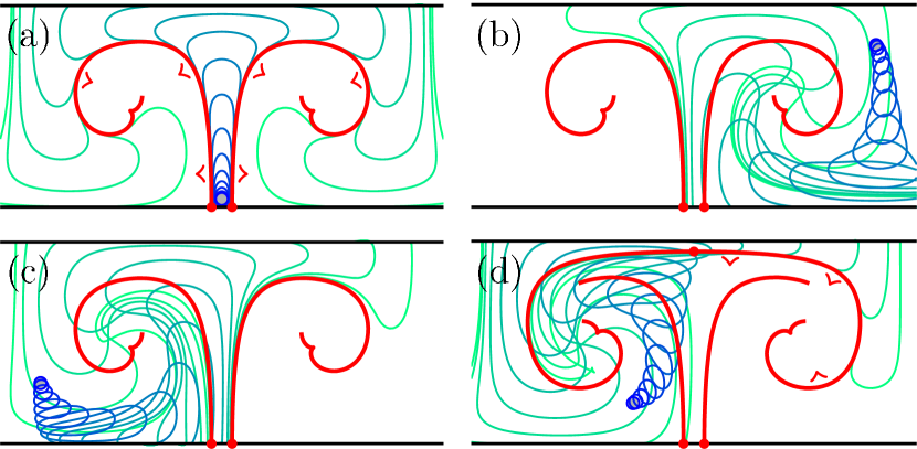
Figure 1: (color online) a) Fronts converging (blue to green) upon BIMs (bold, red) in a time-independent vortex flow. Panels b–d show fronts initialized at different stimulation points (small open circles) burning through BIMs opposite their burning direction but bounded by BIMs in their burning direction. Panel d includes a BIM attached to a burning fixed point near the top of the channel, which restricts the front in the upper right.

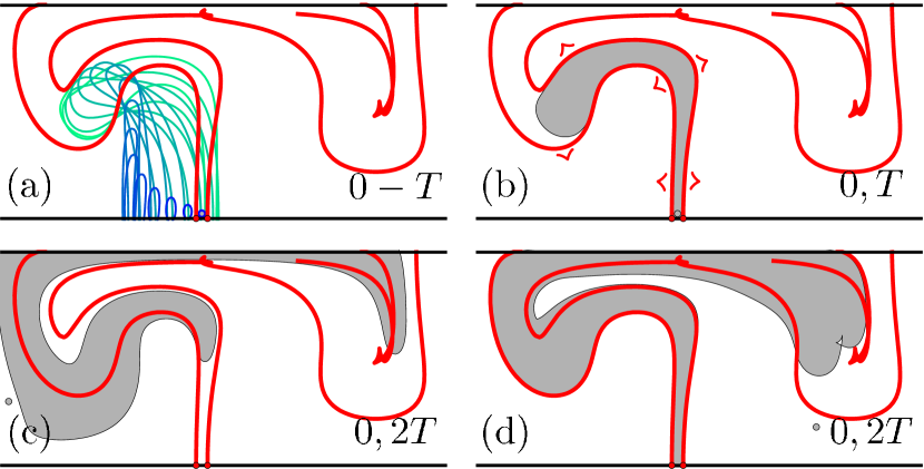
Figure 2: (color online) BIMs in a time-periodic flow. An initial stimulation between the BIMs moves outside the BIMs during the forcing cycle (panel a) but returns by time $T$ (panel b). A stimulation to the left of the BIM pair evolves through one BIM but not the other (panel c). Similarly for a stimulation on the right (panel d).

We give a brief overview of the physical role played by BIMs. Figure 1 illustrates the BIMs (bold, red) for a time-independent flow, confined to a horizontal channel with counter-rotating vortices. In Fig. 1a, the reaction is catalyzed at the channel bottom between the BIMs, and then generates the sequence of reaction fronts, forming an upward propagating plume, ultimately rolled up by the vortices. The fronts are bounded by the BIMs on either side, with the arrows normal to the BIMs denoting the “burning” direction of each BIM. A BIM forms a barrier to fronts propagating in its burning direction (as in Fig. 1a), but not to fronts impinging in the opposite direction, as illustrated in Figs. 1b–d. In Figs. 1b–d the fronts are catalyzed at different stimulation points (small open circles) and approach the BIMs from different directions. In each case, the fronts pass through a BIM when approaching opposite the BIM’s burning direction but are stopped when approaching in the burning direction.

In Fig. 2, the vortices oscillate periodically in the horizontal direction. The BIMs are shown at a single phase of the driving only. An initial stimulation between the BIMs in Fig. 2a grows outward in a series of reaction fronts. During the first period, the front migrates outside the BIM channel in Fig. 2a, but returns to it exactly one driving period $T$ after initialization (shown by the gray “burned” region in Fig. 2b.) Figures 2c and 2d show two additional stimulation points, and their subsequent evolution after two driving periods (in gray). In both cases, BIMs bound the front evolution in their burning direction, but not in the opposite direction.

This paper is organized as follows. Section II.1 introduces the finite-dimensional dynamical system for a point along the front, and Sec. II.2 discusses how extended fronts are represented within this framework. Section II.4 compares this ODE approach to a grid-based computation. Front singularities and collisions are discussed in Sec. II.5. Section II.6 formalizes the observation that fronts cannot pass one another, in what we call the “no-passing” lemma. Section III derives existence (Sec. III.1) and stability (Sec. III.3) results for fixed points of the front dynamics, focusing on time-independent flows. Linear flows are examined in Sec. III.2. The existence of fixed points is constrained by a topological index theory developed in Sec. III.4. The heart of the paper is the introduction of BIMs in Sec. IV, which establishes that BIMs can (locally) be interpreted as fronts (Sec. IV.1) that provide one-sided barriers to front propagation (Sec. IV.2). Sections IV.3 and IV.4 discuss two mechanisms for circumventing these barriers. Section IV.5 describes how BIMs attract fronts, providing a mechanism to measure BIMs directly in the laboratory. Finally, Sec. V connects features of BIMs to the geometry of the simpler cases of either pure (passive) advection or pure (nonadvecting) front propagation.

II Front propagation in an advecting medium: fundamental concepts

We analyze the general problem of a front propagating through a two-dimensional medium flowing with velocity $\mathbf{u}(\mathbf{r},t)$, specified as a function of position $\mathbf{r}=(x,y)$ and time $t$. In the local co-moving frame of the medium, propagation is assumed to progress normal to the front at a speed $v_{0}$ (the burning speed), which is constant, independent of position, propagation direction, or the local front curvature ¹⁵. Finally, the velocity field $\mathbf{u}(\mathbf{r},t)$ is assumed to be established independently from the front dynamics itself, i.e. the development of the front does not feedback to modify $\mathbf{u}$.

Our front propagation theory has been successfully applied to the driven advection-reaction-diffusion (ARD) systems studied experimentally by Solomon ^{20; 18}. In these experiments, the reaction time scale is much faster than the advection time scale (i.e. large Damköhler number), meaning that the front is thin compared to the scale of the flow—the so-called “geometric optics” limit ²⁸. In this limit, a fluid element is either fully reacted or unreacted; hence, the distribution of reaction products within the fluid is entirely determined by the boundary of the reacted, or “burned”, region. Throughout this paper, such ARD systems form the prototype example, though our theoretical framework should lend insight into pattern formation in other systems that combine front propagation and advection, including not only chemical reaction dynamics, but optics, phase-transitions, and even quantum phenomena.

II.1 A three-dimensional ODE for the propagation of front elements in a two-dimensional flow

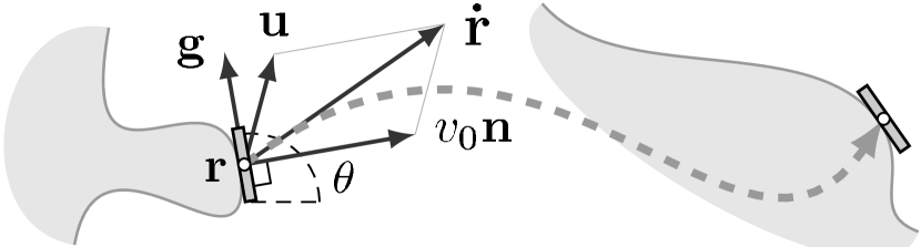
Figure 3: Each reaction front element independently propagates forward under the ODEs (4) and (5).

A front element, i.e. a point on the boundary between burned and unburned regions, is described by both its position $\mathbf{r}=(x,y)$ and its unit normal $\mathbf{n}$ (Fig. 3). Alternatively, $\mathbf{n}$ can be replaced by the unit tangent $\mathbf{g}$, defined here by a right-handed turn by $\pi/2$,

$$\mathbf{g}=\mathsf{J}\mathbf{n}, \quad\text{where}\quad\mathsf{J}=\left[\begin{array}[]{cc}0&-1\\ 1&0\end{array}\right].$$ (3)

Under the above assumptions, a front element evolves via ³⁵

$$\mathbf{\dot{r}} =\mathbf{u}+v_{0}\mathbf{n}$$ (4a)

$$=\mathbf{u}-v_{0}\mathsf{J}\mathbf{g},$$ (4b)

$$\mathbf{\dot{g}} =[\mathbf{g}\cdot(\nabla\mathbf{u})\mathbf{n}]\mathbf{n}$$ (4c)

$$=\mathbf{g}\cdot(\nabla\mathbf{u})-[\mathbf{g}\cdot(\nabla\mathbf{u})\mathbf{g}]\mathbf{g},$$ (4d)

where dots denote time derivatives and $\nabla\mathbf{u}$ is the velocity gradient tensor with components $(\nabla\mathbf{u})_{ij}=u_{j,i}$, $i,j=x,y$, where a comma denotes partial differentiation. The equivalence of Eqs. (4a) and (4b) and of Eqs. (4c) and (4d) is straightforward, the latter requiring $|\mathbf{g}|=1$. To justify Eqs. (4a) and (4d), first consider the nonburning case $v_{0}=0$ for which front elements should evolve under advection alone. Equation (4a) reduces to the appropriate advective form $\mathbf{\dot{r}}=\mathbf{u}$. Eq. (4d) remains unchanged; the first term generates the dynamics of advection on the (unnormalized) tangent vector, whereas the second enforces the normalization $|\mathbf{g}|=1$. [Equation (4d) readily yields $d|\mathbf{g}|^{2}/dt=2\mathbf{g}\cdot\mathbf{\dot{g}}=0$ when $|\mathbf{g}|=1$.] Considering the case $v_{0}\neq 0$, the only necessary change to Eqs. (4a) and (4d) is to add the burning velocity $v_{0}\mathbf{n}$ normal to the front in Eq. (4a). An appealing physical analogy can be obtained by recognizing that Eq. (4) also describes the motion of a thin rod-shaped swimmer aligned with $\mathbf{g}$ and propelling itself normal to its alignment direction at constant speed $v_{0}$ in the local fluid frame.

Since $|\mathbf{g}|=1$ for all time, Eq. (4) reduces to a three-dimensional ODE in $(x,y,\theta)$, where $\theta$ is the orientation angle between $\mathbf{g}$ and the positive $x$-axis (Fig. 3), i.e. $\mathbf{g}=(\cos\theta,\sin\theta)$.

$$\displaystyle\dot{x} =u_{x}+v_{0}\sin{\theta},$$ (5a)

$$\dot{y} =u_{y}-v_{0}\cos{\theta},$$ (5b)

$$\displaystyle\dot{\theta} =-u_{x,x}\sin{\theta}\cos{\theta}-u_{x,y}\sin^{2}{\theta}+$$

$$\quad u_{y,x}\cos^{2}{\theta}+u_{y,y}\sin{\theta}\cos{\theta}.$$ (5c)

For incompressible fluids, $u_{y,y}=-u_{x,x}$, simplifying Eq. (5c). We emphasize that even though Eq. (5) is three-dimensional, the fluid flow itself is two-dimensional. The reduction from four [Eq. (4)] to three [Eq. (5)] dimensions is useful for both numerical computations and many theoretical arguments.

II.2 Front compatibility criterion

A front may either be viewed as a curve in the two-dimensional $xy$-space or in the three-dimensional $xy\theta$-space (or indeed even in the four-dimensional $\mathbf{rg}$-space.) We clarify the relationship between these two representations here. First, we parameterize fronts by their Euclidean length $\lambda$, measured along the front in $xy$-space. By convention $\lambda$ increases in the $+\mathbf{g}$ direction; this is equivalent to keeping the burned region on your left while traversing the curve. Then any (differentiable) curve $\mathbf{r}(\lambda)$ representing a front in $xy$-space lifts to a unique curve $(\mathbf{r}(\lambda),\theta(\lambda))$ in $xy\theta$-space, where $\theta(\lambda)$ is the unique (modulo $2\pi$) solution to

$$(\cos\theta(\lambda),\sin\theta(\lambda))=d\mathbf{r}/d\lambda.$$ (6)

On the other hand, a general curve $(\mathbf{r}(\lambda),\theta(\lambda))$ in $xy\theta$-space is typically not the lift of a curve in $xy$-space—only those curves in $xy\theta$-space satisfying Eq. (6) represent fronts. We thus call Eq. (6) the front compatibility criterion for a curve $(\mathbf{r}(\lambda),\theta(\lambda))$. Geometrically, it is the requirement that at every point $\lambda$ of the curve, the two-dimensional vector $d\mathbf{r}/d\lambda$ points in the direction $\mathbf{g}(\lambda)$, defined by $\mathbf{g}(\lambda)=(\cos\theta(\lambda),\sin\theta(\lambda))$. Thus the front compatibility criterion is equivalently written

$$\mathbf{g}\cdot\mathsf{J}\frac{d\mathbf{r}}{d\lambda}=\mathbf{n}\cdot\frac{d\mathbf{r}}{d\lambda}=0.$$ (7)

For curves in $xy\theta$-space, we reserve the term front for those curves satisfying the front compatibility criterion. To summarize, a front is represented either by a parameterized curve in $xy$-space or a parameterized curve in $xy\theta$-space that satisfies the front compatibility criterion, and there is a one-to-one correspondence between these representations.

If the front compatibility criterion [Eq. (7)] holds along a curve $(\mathbf{r}(\lambda,t),\theta(\lambda,t))$ at some initial time, then it must hold for all future times as the curve evolves. Physically, this must be the case, since the time-evolution of a front must remain a front. To check that it follows from Eq. (4), assume first that Eq. (7) holds at an initial time. Then,

$$\frac{d}{dt} \left(\mathbf{g}\cdot\mathsf{J}\frac{d\mathbf{r}}{d\lambda}\right)$$

$$=[\mathbf{g}\cdot(\nabla\mathbf{u})\mathbf{n}]\mathbf{n}\cdot\mathsf{J}\frac{d\mathbf{r}}{d\lambda}+\mathbf{g}\cdot\mathsf{J}\left[(\nabla\mathbf{u})^{T}\frac{d\mathbf{r}}{d\lambda}-v_{0}\mathsf{J}\frac{d\mathbf{g}}{d\lambda}\right]$$

$$=-\mathbf{g}\cdot(\nabla\mathbf{u})\mathbf{n}+\mathbf{n}\cdot(\nabla\mathbf{u})^{T}\mathbf{g}=0,$$ (8)

where the first equality follows from Eq. (4) and the second from the fact that $\mathbf{g}\cdot(d\mathbf{g}/d\lambda)=0$ and Eqs. (3) and (6). Thus, if Eq. (7) holds at an initial time, it holds for all future times.

II.3 Example Fluid Flow

Equations (4) and (5) are valid for an arbitrary flow $\mathbf{u}(\mathbf{r},t)$. For illustrative purposes (see Figs. 1, 2, 4, 10, and 11), we use the following incompressible velocity field

$$u_{x}(x,y,t) =+\sin(\pi[x+b\sin(\omega t)])\cos(\pi y),$$ (9)

$$u_{y}(x,y,t) =-\cos(\pi[x+b\sin(\omega t)])\sin(\pi y).$$

This flow represents an array of alternating vortices, periodically driven with frequency $\omega$ and amplitude $b$. It has been extensively used to successfully model driven laboratory flows ^{36; 37; 38; 22; 23; 18; 20 39}.

II.4 Two approaches to front propagation: curve-based versus grid-based

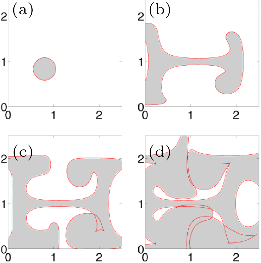
Figure 4: a) An initial circular burned region at $t=0.25T$, with the black front surrounding it; Panels b–d show the forward evolution at times $t=0.69T,0.97T,1.16T$. The black front is evolved using Eq. (5) with $v_{0}=0.2$ and $\mathbf{u}$ given by Eq. (9), with $b=0.25$, and $\omega=2$. The gray burned domain is evolved according to a grid-based, split-step algorithm, using 1668x1668 grid points within the $xy$-domain shown (full integration domain is larger), with time step $\Delta t=2\pi/(32\omega)$.

Under the assumptions laid out in Sec. II.1, an entire front can be evolved by independently evolving individual front elements. Numerically, this requires a sufficient density of points along the front to resolve it to a desired accuracy. As the front evolves, the separation between some of the points typically increases, requiring the addition of new interpolated points to maintain sufficient density. We use an algorithm similar to Ref. (40).

Refs. (41; 42; 38) used a Euclidean-grid-based approach to evolve the entire burned region itself. In such an approach, each grid point is recorded as either burned or unburned at a given time. A split-step scheme, consisting of a pure burning step and a pure advection step, is used to update each gridpoint in time. (For details, see Refs. (41; 42; 38).) In contrast, our approach focuses solely on the front itself.

Fig. 4 compares the above two algorithms for front evolution. Fig. 4a shows an initial burned circular region. The black curve denotes the front $(x(\lambda),y(\lambda),\theta(\lambda))$ that forms the initial condition (at $t=0.25T$, with $T=2\pi/\omega$) for evolution via Eqs. (5) and (9). A corresponding grid-based computation is also performed, with initial condition consisting of the burned grid points inside the circle (shaded gray.) Fig. 4b shows the independent evolution of both the black circle [via Eq. (5)] and the gray grid points [via the split-step algorithm] up to $t=0.69T$. The two techniques agree well, with the black curve marking the boundary of the gray region, thereby providing added numerical confirmation for the validity of Eq. (5). The tiny visible discrepancy is due to the finite grid resolution.

II.5 Front intersections and cusps

Fig. 4c continues the evolution to $t=0.97T$. Part of the evolved front now lies within the burned (gray) region. While we refer to the entire evolved curve (either in $xy$-space or $xy\theta$-space) as the front, we refer to those segments of the front separating the burned from unburned regions as the bounding front; those intervals of the front not in the bounding front thus lie interior to the burned region. Note that the bounding front need not be connected, but can have disconnected segments defining voids, as seen at time $t=1.16T$ (Fig. 4d). Figures 4c and 4d continue the excellent agreement between the evolution algorithms. Note that even though the front may intersect itself when projected into the $xy$-plane, it cannot self intersect in the full $xy\theta$-space, as mandated by the uniqueness theorem for solutions of ODEs.

Figures 4c and 4d illustrate two mechanisms by which a front may penetrate the interior of the burned region. In the transition from Fig. 4b to Fig. 4c, a so-called swallowtail catastrophe is formed by the $xy$-projection of the front ^{43; 44}; the characteristic swallowtail shape, with its two cusps, is seen interior to the burned region in Fig. 4c. Despite singularities in its $xy$-projection, the front in $xy\theta$-space remains smooth throughout. In the transition from Fig. 4c to Fig. 4d, fronts penetrate the interior through the head-on collision of distinct locations along the front. Both mechanisms for producing front intersections in the $xy$-plane are characteristic of front evolution in optics ^{43; 44}, for example, and do not require the presence of advection.

II.6 Front no-passing lemma

Consider two fronts, with one front trailing the other. Since both fronts have the same speed in the local fluid frame, it is clear that the trailing front can not catch up to and pass the leading front. This no-passing result will be central to understanding why BIMs form one-sided barriers to front evolution in Sec. IV.

The intuitive no-passing statement above can be recast more precisely as follows. Let $C_{0}$ and $C_{0}^{\prime}$ be the leading and trailing fronts, and assume that they are represented by (piecewise smooth) nonintersecting closed loops in $xy$-space, with $C_{0}^{\prime}$ nested inside $C_{0}$ (Fig. 5a). Without loss of generality, we assume that both are burning outward, meaning that their interior domains are burned. (The case of both burning inward, with their interior domains unburned, can be handled analogously.) The fronts may extend to infinity or coincide with a boundary wall for part of their length, so long as the burned region of $C_{0}^{\prime}$ is entirely included within the burned region of $C_{0}$. As $C_{0}$ and $C_{0}^{\prime}$ evolve forward for some time $t$, according to Eq. (5), they produce new fronts $C_{t}$ and $C_{t}^{\prime}$. In general, $C_{t}$ and $C_{t}^{\prime}$ might self-intersect and intersect one another (in the $xy$-plane), as shown in Fig. 5a. However, despite these intersections, the bounding fronts $\bar{C}_{t}$ and $\bar{C}_{t}^{\prime}$ (in bold) will not intersect and will retain their original nested ordering, with $\bar{C}_{t}^{\prime}$ lying within the burned region defined by $\bar{C}_{t}$. We call this the no-passing lemma. It follows from the simple physical observation that the innermost burned region must always remain a subset of the outermost burned region.

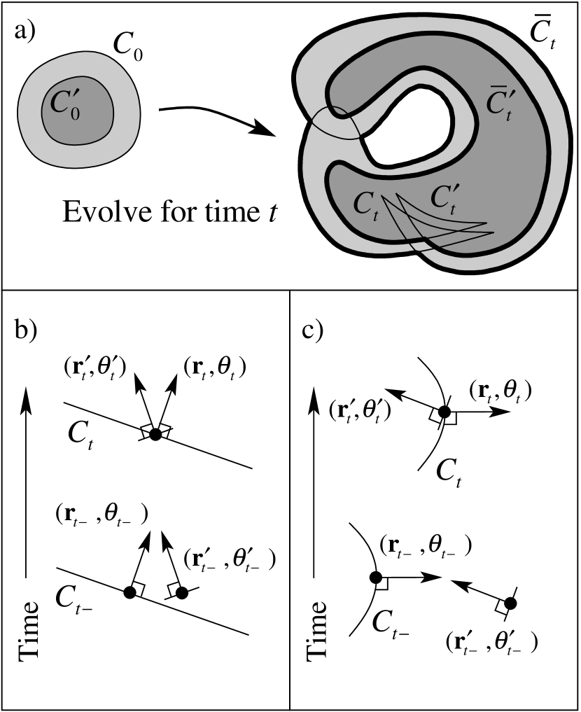
Figure 5: a) The fronts $C_{0}$ and $C_{0}^{\prime}$ evolve into $C_{t}$ and $C_{t}^{\prime}$. The bounding fronts $\bar{C}_{t}$ and $\bar{C}_{t}^{\prime}$ (in bold) have the same nested ordering as $C_{0}$ and $C_{0}^{\prime}$. Panels b and c illustrate a front element $(\mathbf{r}_{t}^{\prime},\theta^{\prime})$ (of $C_{t}^{\prime}$, not shown) approaching $C_{t}$ from the front and colliding with it.

The no-passing lemma can be recast as a local formulation in terms of non-closed segments of the fronts $C_{t}$ and $C_{t}^{\prime}$. Suppose $(\mathbf{r}_{t}^{\prime},\theta^{\prime}_{t})$ is a front element (of curve $C_{t}^{\prime}$) whose position $\mathbf{r}_{t}^{\prime}$ coincides with a point $\mathbf{r}_{t}$ on the front $C_{t}$, but whose $\theta^{\prime}_{t}$ does not agree with the local orientation of $C_{t}$. Then a short time $\epsilon$ earlier, the front element $(\mathbf{r}_{t-\epsilon}^{\prime},\theta^{\prime}_{t-\epsilon})$ must lie in front of $C_{t-\epsilon}$ (Figs. 5b and 5c). Said another way, the front element $(\mathbf{r}_{t}^{\prime},\theta^{\prime}_{t})$ can not catch up to and pass $C_{t}$ from behind. Of course, there is nothing preventing $(\mathbf{r}_{t}^{\prime},\theta^{\prime}_{t})$ from colliding with $C_{t}$ from the front, as in Figs. 5b and 5c. Formally, the local no-passing formulation may be recast as the inequality

$$\dot{\mathbf{r}}^{\prime}\cdot\mathbf{n}<\dot{\mathbf{r}}\cdot\mathbf{n},$$ (10)

where $\dot{\mathbf{r}}^{\prime}$ and $\dot{\mathbf{r}}$ are the velocities of the two front elements at the time their $xy$-positions coincide and $\mathbf{n}$ is the unit normal to $C_{t}$. Equation (10) follows directly from $\dot{\mathbf{r}}=\mathbf{u}(\mathbf{r})+v_{0}\mathbf{n}$ [Eq. (4a)], $\dot{\mathbf{r}}^{\prime}=\mathbf{u}(\mathbf{r})+v_{0}\mathbf{n}^{\prime}$, and $\mathbf{n}\cdot\mathbf{n^{\prime}}<1$. Finally, note that the roles of $(\mathbf{r}_{t}^{\prime},\theta^{\prime}_{t})$ and $(\mathbf{r}_{t},\theta_{t})$ can be reversed, so that $(\mathbf{r}_{t},\theta_{t})$ can not catch up to and pass $C_{t}^{\prime}$ either; mathematically, $\dot{\mathbf{r}}\cdot\mathbf{n}^{\prime}<\dot{\mathbf{r}}^{\prime}\cdot\mathbf{n}^{\prime}.$

III Burning fixed points

By a burning fixed point, we mean either an equilibrium point of the differential equation (4) [or (5)], for time-independent flows, or a fixed point of the corresponding Poincaré map, for time-periodic flows. For the remainder of Sec. III, we restrict our focus to time-independent flows, for which we give a precise characterization of the existence and stability of burning fixed points.

III.1 Existence criteria for burning fixed points in time-independent flows

At a burning fixed point in a time-independent flow, Eq. (4a) implies $v_{0}\mathbf{n}=-\mathbf{u}$, so that the fluid velocity is exactly balanced by the burning velocity. Eq. (4c) on the other hand implies $0=\mathbf{n}\cdot\mathbf{\dot{g}}=\mathbf{g}\cdot(\nabla\mathbf{u})\mathbf{n}$.

Theorem 1

A burning fixed point $(\mathbf{r},\mathbf{g})$ occurs if and only if the following two conditions are met.

$$(i)\quad v_{0}\mathbf{n} =-\mathbf{u},$$ (11)

$$(ii)\quad \mathbf{g}\cdot(\nabla\mathbf{u})\mathbf{n} =0.$$ (12)

Condition (ii) is equivalent to

$$(ii^{\prime})\quad(\nabla\mathbf{u})^{T}\mathbf{g}=\mu\mathbf{g},$$ (13)

for some (necessarily real) eigenvalue $\mu$.

Figure 6: Illustration of flows with $\mu>0$ and $\mu<0$ about a burning fixed point, at which $\mathbf{u}$ is normal to the set $\mathcal{C}$ defined by $|\mathbf{u}|=v_{0}$. The burning direction $\mathbf{n}$ points opposite $\mathbf{u}$.

Together, Eqs. (11) and (12) imply $\mathbf{g}\cdot\nabla|\mathbf{u}|^{2}=0,$ i.e. $\mathbf{g}$ is tangent to the level set $|\mathbf{u}|=v_{0}$ (assuming $\nabla|\mathbf{u}|^{2}\neq 0$). Alternatively, $\mathbf{n}$ is normal to the level set, so that by Eq. (11) $\mathbf{u}$ is also normal to the level set.

Theorem 2

Define the level set $\mathcal{C}$ in $xy$-space by $|\mathbf{u}|=v_{0}$. Assuming $\nabla|\mathbf{u}|^{2}\neq 0$ on $\mathcal{C}$, the set of burning fixed points consists of exactly those points $(\mathbf{r},\mathbf{g})$ at which $\mathbf{r}$ is on $\mathcal{C}$ and $\mathbf{u}(\mathbf{r})$ points normal to $\mathcal{C}$. The burning direction $\mathbf{n}=-\mathsf{J}\mathbf{g}$ points opposite $\mathbf{u}$.

Figure 6 illustrates Theorem 2 for $\mu>0$ and $\mu<0$.

III.2 Burning fixed points for linear fluid flows

The case of linear flows lends insight into the existence and local structure of burning fixed points.

III.2.1 Hyperbolic flows

The hyperbolic flow

$$u_{x}=-Ax,\quad u_{y}=+Ay,$$ (14)

with strength $A>0$, has a unique hyperbolic advective fixed point at the origin. This flow generates the burning dynamics

$$\dot{x} =-Ax+v_{0}\sin\theta,$$ (15a)

$$\dot{y} =+Ay-v_{0}\cos\theta,$$ (15b)

$$\dot{\theta} =+2A\cos\theta\sin\theta.$$ (15c)

Thus, any fixed point $(x_{*},y_{*},\theta_{*})$ must have $\theta_{*}=0,\pi,\pi/2,3\pi/2$. Each $\theta_{*}$ then yields a unique value of $x_{*}$ and $y_{*}$, summarized in Table 1. The advective hyperbolic fixed point thus produces four burning fixed points as $v_{0}$ deviates from 0.

	BFP $(x_{*},y_{*},\theta_{*})$	Eigenvalues	Stability	1D BIM dir
1	$(0,v_{0}/A,0)$	$-A,+A,+2A$	SUU	$\mathbf{\hat{x}}$
2	$(0,-v_{0}/A,\pi)$	$-A,+A,+2A$	SUU	$\mathbf{\hat{x}}$
3	$(v_{0}/A,0,\pi/2)$	$-A,+A,-2A$	SSU	$\mathbf{\hat{y}}$
4	$(-v_{0}/A,0,3\pi/2)$	$-A,+A,-2A$	SSU	$\mathbf{\hat{y}}$

Table 1: Burning fixed points for hyperbolic flow Eq. (14).

Figure 7a shows the four burning fixed points. Consistent with Theorem 2, these four points lie on the circle $A|\mathbf{r}|=|\mathbf{u}|=v_{0}$, bounding the shaded region $|\mathbf{u}|<v_{0}$. Furthermore, these are exactly the four points where the hyperbolic flow is normal to the circle.

The linearization of Eq. (15) yields

$$\mathsf{L}=\frac{\partial(\dot{x},\dot{y},\dot{\theta})}{\partial(x,y,\theta)}=\left(\begin{array}[]{ccc}-A&0&v_{0}\cos\theta\\ 0&A&v_{0}\sin\theta\\ 0&0&2A\cos 2\theta\end{array}\right).$$ (16)

The eigenvalues of $\mathsf{L}$ at the burning fixed points are $(-A,A,\pm 2A)$, summarized in Table 1. Each fixed point is hyperbolic with either stability stable-stable-unstable (SSU) or stable-unstable-unstable (SUU). Each fixed point with SSU (SUU) stability thus has a one-dimensional unstable (stable) invariant manifold, which is a burning invariant manifold (BIM). These manifolds have eigendirections $(\mathbf{\hat{y}},0)$ (for SSU) or $(\mathbf{\hat{x}},0)$ (for SUU). In both cases, the $xy$-projection of the eigendirection is aligned with the orientation $\mathbf{g}$ of the fixed point.

Focusing on the two burning fixed points on the $x$-axis, their unstable BIMs are the straight lines $\{(\pm v_{0}/A,y,\pi/2)|-\infty<y<\infty\}$, which project to the two vertical lines in Fig. 7a. Note that these BIMs satisfy the front compatibility condition Eq. (6), a point we return to in Sec. IV.1.

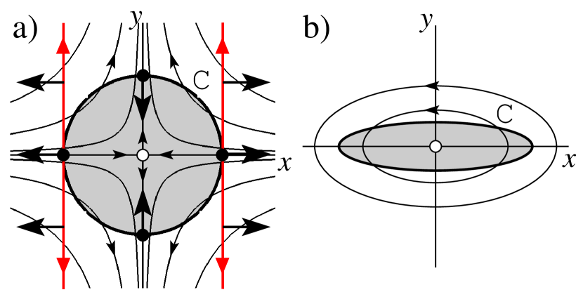
Figure 7: (color online) a) The four burning fixed points (filled dots) in a hyperbolic flow lie on the circle $\mathcal{C}$ (the level set $|\mathbf{u}|=v_{0}$) which surrounds the advective fixed point (open dot). The shaded region satisfies $|\mathbf{u}|<v_{0}$. The burning velocities (large arrows) of these four points are normal to the circle, pointing opposite the flow. The left and right points have stability SSU, and the vertical lines passing through them are their unstable BIMs. The triangular (unbarbed) arrows denote the unstable direction along the BIMs. b) An elliptic flow has no burning fixed points since the flow lines are never normal to the ellipse $\mathcal{C}$ bounding the shaded region.

III.2.2 Elliptic flows

The elliptic flow

$$u_{x}=y/A,\quad u_{y}=-Ax,$$ (17)

with $A>0$, has a unique elliptic advective fixed point at the origin. It generates the burning dynamics,

$$\dot{x} =y/A+v_{0}\sin\theta,$$ (18a)

$$\dot{y} =-Ax-v_{0}\cos\theta,$$ (18b)

$$\dot{\theta} =-(\sin^{2}\theta)/A-A\cos^{2}\theta,$$ (18c)

from which we see that $\dot{\theta}=0$ has no solutions, and hence there are no burning fixed points in a purely elliptic flow. This can also be seen as a consequence of Theorem 2, as illustrated in Fig. 7b. Any burning fixed point must lie on the elliptic level set $[(Ax)^{2}+(y/A)^{2}]^{1/2}=|\mathbf{u}|=v_{0}$ bounding the shaded region. However, the flow is never normal to this set, and hence there are no burning fixed points.

III.3 Stability of burning fixed points for general time-independent flows

For the main results on the stability of burning fixed points, the reader may skip ahead to Theorems 3 and 4. The linearization of Eq. (4) yields the following four-by-four matrix, decomposed into two-by-two blocks.

$$\mathsf{X}=\left(\begin{array}[]{c|c}\partial\mathbf{\dot{r}}/\partial\mathbf{r}&\partial\mathbf{\dot{r}}/\partial\mathbf{g}\\ \hline\cr\partial\mathbf{\dot{g}}/\partial\mathbf{r}&\partial\mathbf{\dot{g}}/\partial\mathbf{g}\end{array}\right)=\left(\begin{array}[]{c|c}(\nabla\mathbf{u})^{T}&-v_{0}\mathsf{J}\\ \hline\cr\mathbf{n}\otimes\mathbf{a}&\mathsf{D}\end{array}\right),$$ (19)

where

$$\mathsf{D} =(\mathbf{g}\otimes\mathbf{n}+\mathbf{n}\otimes\mathbf{g})\left[\mathbf{g}\cdot(\nabla\mathbf{u})\mathbf{n}\right]+$$

$$\mathbf{n}\otimes\mathbf{n}\left[\text{Tr}(\nabla\mathbf{u})-2\mathbf{g}\cdot(\nabla\mathbf{u})\mathbf{g}\right],$$ (20)

$$\mathbf{a} =\mathbf{g}\cdot\nabla\nabla(\mathbf{n}\cdot\mathbf{u}).$$ (21)

Here, a tensor product $\mathbf{b}\otimes\mathbf{c}$ has components $(\mathbf{b}\otimes\mathbf{c})_{ij}=b_{i}c_{j}$ and $a_{i}=g_{k}n_{j}u_{j,ki}$, where repeated indices are summed according to the Einstein convention.

We now specialize to linearization about a burning fixed point for time-independent flows, and assume $\nabla|\mathbf{u}|^{2}\neq 0$. Equations (11) – (13) imply

$$\mathsf{D}=\mathbf{n}\otimes\mathbf{n}\left[\text{Tr}(\nabla\mathbf{u})-2\mu\right].$$ (22)

Now, since $|\mathbf{g}|=1$ is preserved by the dynamics, we need only consider variations of $\mathbf{g}$ in the direction $\mathbf{n}$; i.e. we consider the three-dimensional space of vectors of the form $(\mathbf{v},c\mathbf{n})$, with $\mathbf{v}\in\mathbb{R}^{2}$ and $c\in\mathbb{R}$, which is invariant under $\mathsf{X}$. Restricting $\mathsf{X}$ to this space yields the three-by-three matrix

$$\mathsf{Y}=\left(\begin{array}[]{cc}(\nabla\mathbf{u})^{T}&-v_{0}\mathbf{g}\\ \mathbf{a}^{T}&\text{Tr}(\nabla\mathbf{u})-2\mu\end{array}\right).$$ (23)

Equation (13) implies that the two-dimensional space of vectors of the form $(a\mathbf{g},c)$, with $a,c\in\mathbb{R}$, is invariant under $\mathsf{Y}$. Restricting $\mathsf{Y}$ to this space yields the two-by-two matrix

$$\mathsf{Z}=\left(\begin{array}[]{cc}\mu&-v_{0}\\ \mathbf{a}\cdot\mathbf{g}&\text{Tr}(\nabla\mathbf{u})-2\mu\end{array}\right).$$ (24)

The eigenvalue of $\mathsf{Y}$ whose eigenvector does not have the form $(a\mathbf{g},c)$ is thus

$$\lambda_{0}=\text{Tr}(\mathsf{Y})-\text{Tr}(\mathsf{Z})=\text{Tr}(\nabla\mathbf{u})-\mu=\nu,$$ (25)

where $\nu$ is the remaining (necessarily real) eigenvalue of $(\nabla\mathbf{u})^{T}$. The remaining two eigenvalues of $\mathsf{Y}$ are thus the two eigenvalues of $\mathsf{Z}$ given by

$$\lambda_{\pm}=\frac{1}{2}\left(\nu\pm\sqrt{\nu^{2}-4[v_{0}\mathbf{a}\cdot\mathbf{g}+\mu(\nu-\mu)]}\right).$$ (26)

This expression can be put in a simpler form if we first consider the components of $\mathbf{u}$ in the local frame of $\mathcal{C}$ (the level set $|\mathbf{u}|=v_{0})$, defined by $\mathbf{e}_{1}^{\prime}$ and $\mathbf{e}_{2}^{\prime}$, the unit normal and tangent vectors to $\mathcal{C}$, respectively. The components of $\mathbf{u}$ in the $(\mathbf{e}_{1}^{\prime},\mathbf{e}_{2}^{\prime})$ frame are denoted $\mathbf{u}^{\prime}=(u_{1}^{\prime},u_{2}^{\prime})$. We parameterize $\mathcal{C}$ by the Euclidean distance $\lambda$ measured along $\mathcal{C}$. At a burning fixed point, the derivative of $\mathbf{u}$ along $\mathcal{C}$ is thus $d\mathbf{u}/d\lambda$, which by Eq. (13) equals $\mu\mathbf{g}$, taking $\lambda$ to increase in the direction $\mathbf{g}$. The quantity $\mu/v_{0}=\mu/|\mathbf{u}|$ is thus a kind of rotation rate of $\mathbf{u}$ along $\mathcal{C}$. Similarly, we may differentiate $\mathbf{u}$ in the $(\mathbf{e}_{1}^{\prime},\mathbf{e}_{2}^{\prime})$ frame, i.e. $d\mathbf{u^{\prime}}/d\lambda$. Since $|\mathbf{u^{\prime}}|=v_{0}$ is constant along $\mathcal{C}$, $d\mathbf{u^{\prime}}/d\lambda$ must point orthogonal to $\mathbf{u^{\prime}}$. At a burning fixed point, $\mathbf{g}$ is orthogonal to $\mathbf{u}$, and hence

$$d\mathbf{u^{\prime}}/d\lambda=\mu^{\prime}\mathbf{g^{\prime}},$$ (27)

where $\mathbf{g^{\prime}}=(0,1)$ is the components of $\mathbf{g}$ in the $(\mathbf{e}_{1}^{\prime},\mathbf{e}_{2}^{\prime})$ frame. The (real) quantity $\mu^{\prime}/v_{0}$ is thus also the rotation rate of $\mathbf{u}$ along $\mathcal{C}$, but viewed in the $(\mathbf{e}_{1}^{\prime},\mathbf{e}_{2}^{\prime})$ frame. Appendix A shows

$$\mu^{\prime}=\mu+v_{0}\kappa,$$ (28)

where $\kappa$ is the (signed) curvature of $\mathcal{C}$, which equals (see Appendix A)

$$\kappa=\frac{v_{0}\mathbf{a}\cdot\mathbf{g}-\mu^{2}}{v_{0}\nu}$$ (29)

at a burning fixed point. Combining Eqs. (28) and (29) yields

$$\mu^{\prime}=\frac{1}{\nu}\left[v_{0}\mathbf{a}\cdot\mathbf{g}+\mu(\nu-\mu)\right],$$ (30)

which can be used to transform Eq. (26), as below.

Theorem 3

For a time-independent flow $\mathbf{u}$, the eigenvalues about a burning fixed point are

$$\lambda_{0} =\nu,$$ (31)

$$\lambda_{\pm} =\frac{1}{2}\left(\nu\pm\sqrt{\nu^{2}-4\nu\mu^{\prime}}\right),$$ (32)

where $\nu$ is the eigenvalue of $(\nabla\mathbf{u})^{T}$ not given by Eq. (13) and $\mu^{\prime}$ is given by Eq. (27). The linear stability of a burning fixed point is thus determined by the signs of $\nu$ and $\mu^{\prime}$ according to the following table.

	$\nu<0$	$\nu>0$
$\mu^{\prime}>0$	SSU	UUU
$\mu^{\prime}<0$	SSS	SUU

In the above, $\nu$ determines the stability of two eigenvalues and $\mu^{\prime}$ the stability of one. In either the SSU or SUU case, all eigenvalues are real. However, in the UUU or SSS case, two eigenvalues are complex if $4\mu^{\prime}/\nu>1$. In Sect. IV we shall pay particular attention to the SSU case. For incompressible flows $\nu=-\mu$, and Eq. (30) reduces to

$$\mu^{\prime}=\frac{1}{\mu}\left[2\mu^{2}-v_{0}\mathbf{a}\cdot\mathbf{g}\right],$$ (33)

and Theorem 3 specializes to the following.

Theorem 4

For a time-independent, incompressible flow $\mathbf{u}$, the eigenvalues about a burning fixed point are

$$\lambda_{0} =-\mu,$$ (34)

$$\lambda_{\pm} =\frac{1}{2}\left(-\mu\pm\sqrt{\mu^{2}+4\mu\mu^{\prime}}\right),$$ (35)

where $\mu$ and $\mu^{\prime}$ are given by Eqs. (13) and (27). The linear stability of a burning fixed point is thus determined by the signs of $\mu$ and $\mu^{\prime}$ according to the following table.

	$\mu>0$	$\mu<0$
$\mu^{\prime}>0$	SSU	UUU
$\mu^{\prime}<0$	SSS	SUU

For a linear flow ($\mathbf{a}=0$), Eqs. (34) and (35) reduce to the eigenvalues in Table 1. More generally, for either sufficiently small $v_{0}$ or sufficiently linear flow ($\mathbf{a}$ small), Eq. (33) shows that $\mu^{\prime}$ has the same sign as $\mu$, and thus a burning fixed point has one of only two stability types: SSU ($\mu>0$) or SUU ($\mu<0$). Referring to Fig. 6, defocusing flows yield SSU and focusing flows SUU, as verified by the fixed points in Fig. 7a.

III.4 Topological index theory for the existence of burning fixed points

The number and stability type of burning fixed points are constrained by a topological index theory similar to the Poincaré index theory for fixed points in two-dimensional flows ⁴⁵. Following Theorem 2, we consider a closed loop $\mathcal{C}$ upon which $|\mathbf{u}|=v_{0}$. Since $|\mathbf{u}|\neq 0$ on this loop, the winding of the orientation of $\mathbf{u}$ can be used to define two topological indices. The first is the usual Poincaré index ⁴⁵.

$$n_{P}(\mathcal{C})=\parbox[t]{346.89731pt}{the number of counterclockwise (ccw) rotations made by $\mathbf{u}$ under one ccw circuit of $\mathcal{C}$.}$$ (36)

Fig. 8 illustrates $n_{P}$ for four example flows. The reader is encouraged to confirm the value of $n_{P}$ cited in each case. Following standard practice, a Poincaré index is also defined for each advective fixed point $\mathbf{z}$ as follows.

$$n_{P}(\mathbf{z})=\begin{cases}+1&\mathbf{z}\text{ elliptic}\\ -1&\mathbf{z}\text{ hyperbolic}\end{cases}$$ (37)

The Poincaré index of the loop $\mathcal{C}$ is then equal to the sum of the Poincaré indices of all the enclosed fixed points

$$n_{P}(\mathcal{C})=\sum_{\text{fixed points }\mathbf{z}}n_{P}(\mathbf{z})=N_{e}-N_{h},$$ (38)

where $N_{e}$ and $N_{h}$ are the number of elliptic and hyperbolic advective fixed points, respectively. The reader can confirm this relationship in Fig. 8.

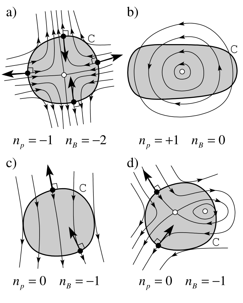
Figure 8: Four flows illustrating Poincaré and burning indices.

Alternatively, by considering the components $\mathbf{u}^{\prime}$ in the local frame $(\mathbf{e}_{1}^{\prime},\mathbf{e}_{2}^{\prime})$ of $\mathcal{C}$, we define the burning index as follows.

$$n_{B}(\mathcal{C})=\parbox[t]{346.89731pt}{the number of ccw rotations made by $\mathbf{u}^{\prime}$ under one ccw circuit of $\mathcal{C}$.}$$ (39)

The two indices are related by

$$n_{B}(\mathcal{C})=n_{p}(\mathcal{C})-1,$$ (40)

since the vector $\mathbf{u}$ in the original laboratory frame undergoes one additional rotation relative to the vector $\mathbf{u}^{\prime}$ in the local frame of $\mathcal{C}$.

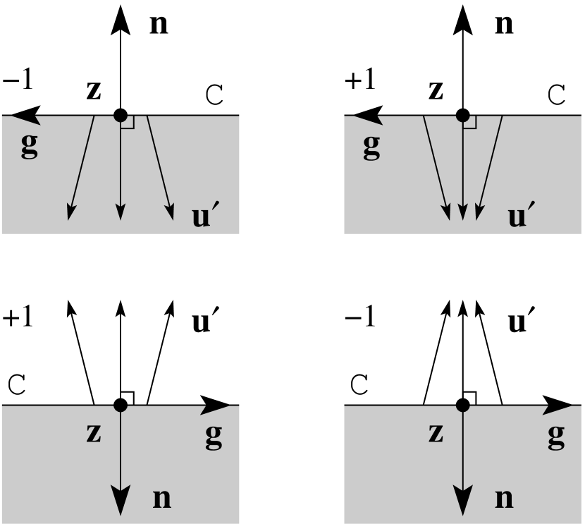
Figure 9: The burning index $\pm 1$ is given for each velocity configuration. The shaded region satisfies $|\mathbf{u}|<v_{0}$.

For each rotation made by $\mathbf{u}^{\prime}$, $\mathbf{u}^{\prime}$ is perpendicular to $\mathcal{C}$ twice, once on either side of $\mathcal{C}$. Thus, there are at least $|n_{B}|$ outward-burning fixed points on $\mathcal{C}$ and $|n_{B}|$ inward-burning fixed points. This result can be refined by defining a burning index for each burning fixed point $\mathbf{z}$.

$$n_{B}(\mathbf{z})=\begin{cases}+1&\mathbf{u^{\prime}}\text{ rotates ccw at }\mathbf{z}\text{, traversing $\mathcal{C}$ ccw}\\ -1&\mathbf{u^{\prime}}\text{ rotates cw at }\mathbf{z}\text{, traversing $\mathcal{C}$ ccw}\end{cases}$$ (41)

This definition is illustrated by the four cases in Fig. 9. These four cases also make it clear that the burning index of a fixed point can be re-expressed in terms of $\mu^{\prime}$ [Eq. (27)] as

$$n_{B}(\mathbf{z})=\begin{cases}\left.\begin{array}[]{ll}+1&\mu^{\prime}<0\\ -1&\mu^{\prime}>0\end{array}\right\}&\parbox{126.47249pt}{and $\mathbf{u}(\mathbf{z})$ points inward to $\mathcal{C}$ (outward-burning)}\\ \\ \left.\begin{array}[]{ll}+1&\mu^{\prime}>0\\ -1&\mu^{\prime}<0\end{array}\right\}&\parbox{126.47249pt}{and $\mathbf{u}(\mathbf{z})$ points outward to $\mathcal{C}$ (inward-burning)}\\ \end{cases}$$ (42)

Analogous to the Poincaré index, the burning index $n_{B}(\mathcal{C})$ of the curve $\mathcal{C}$ is the sum of the burning indices of either all the outward-burning fixed points or all the inward-burning fixed points located on $\mathcal{C}$.

$$n_{B}(\mathcal{C}) =\sum_{\text{out BFPs }\mathbf{z}}n_{B}(\mathbf{z})=N^{\text{out}}_{-}-N^{\text{out}}_{+}$$ (43)

$$=\sum_{\text{in BFPs }\mathbf{z}}n_{B}(\mathbf{z})=N^{\text{in}}_{+}-N^{\text{in}}_{-},$$ (44)

where $N^{\text{out}}_{+}$ and $N^{\text{out}}_{-}$ are the number of outward-burning fixed points with $\mu^{\prime}>0$ and $\mu^{\prime}<0$, respectively, and $N^{\text{in}}_{+}$ and $N^{\text{in}}_{-}$ are the number of inward-burning fixed points with $\mu^{\prime}>0$ and $\mu^{\prime}<0$, respectively. Finally, the number and type of burning fixed points on $\mathcal{C}$ can be directly related to the advective fixed points interior to $\mathcal{C}$ through Eqs. (38) and (40).

$$N^{\text{out}}_{-}-N^{\text{out}}_{+}=N^{\text{in}}_{+}-N^{\text{in}}_{-}=N_{e}-N_{h}-1.$$ (45)

For an incompressible flow, $\mu$ must be positive when $\mathbf{u}$ points inward and negative when $\mathbf{u}$ points outward. Using the table in Theorem 4, Eq. (42) then becomes

$$n_{B}(\mathbf{z})=\begin{cases}\begin{array}[]{ll}+1&\text{stability }SSS\text{ and outward-burning}\\ -1&\text{stability }SSU\text{ and outward-burning}\\ \\ +1&\text{stability }UUU\text{ and inward-burning}\\ -1&\text{stability }SUU\text{ and inward-burning}\end{array}\end{cases}$$ (46)

Similarly, Eq. (45) becomes

$$N^{\text{out}}_{SSS}-N^{\text{out}}_{SSU}=N^{\text{in}}_{UUU}-N^{\text{in}}_{SUU}=N_{e}-N_{h}-1,$$ (47)

where $N^{\text{in/out}}_{XXX}$ measures the number of inward/outward-burning fixed points of the given stability type. This equation is confirmed in Fig. 8, where all burning fixed points either have stability $SSU$ or $SUU$ and hence the number of outward- or inward-burning fixed points simply equals $1-N_{e}+N_{h}=-n_{B}(\mathcal{C})$.

IV Burning invariant manifolds (BIMs): one-sided barriers to front propagation

Having examined the existence and stability of burning fixed points in Sect. III, we now focus on the invariant manifolds attached to them. These manifolds are invariant either under the differential equation (4) [or (5)], in the time-independent case, or under the Poincaré map, in the time-periodic case; a stable/unstable invariant manifold consists of all points that converge upon a burning fixed point in forward/backward time ⁴⁵. As noted above, we call these stable and unstable manifolds burning invariant manifolds (BIMs) to distinguish them from the traditional invariant manifolds for advection. Due to the special role played by one-dimensional invariant manifolds, all BIMs subsequently discussed are assumed to be one-dimensional, unstable manifolds, attached to a fixed point of stability SSU, as shown in Figs. 1 and 2 for time-independent and time-periodic flows. (One-dimensional, stable BIMs are similarly analyzed by running time backwards; they will be relevant in a future publication for developing a theory of lobe dynamics for front propagation.) The central point of our theoretical development is that these BIMs form one-sided barriers to front propagation (Figs. 1 and  2).

IV.1 BIMs are fronts

Though most one-dimensional curves in the three-dimensional $xy\theta$-space are not fronts, an unstable (one-dimensional) BIM attached to an SSU fixed point does satisfy the front compatibility criterion, i.e. Eq. (6) or (7), as established here. Consider first a short line segment $(x_{*},y_{*},\theta_{*})+(\lambda\cos(\theta),\lambda\sin(\theta),0)$, parameterized by $-\epsilon<\lambda<\epsilon$ and passing through a burning fixed point $(x_{*},y_{*},\theta_{*})$ of stability SSU. This line clearly satisfies Eq. (6). Furthermore, due to the two stable dimensions of the fixed point, as this curve evolves in time, it converges upon the BIM, approximating progressively longer segments of the BIM  ⁴⁶ . Since the front compatibility criterion is preserved over time, the evolving curve remains a front, and hence the BIM to which it converges satisfies the front compatibility criterion everywhere along its length. This argument applies for both time-independent and time-periodic flows.

IV.2 BIMs are one-sided barriers

As pointed out in Figs. 1 and 2, BIMs are one-sided barriers, preventing fronts from passing in one direction, but not the other. We can now explain this fact as follows. Since BIMs are fronts, they satisfy the no-passing lemma (Sect. II.6). The local formulation of this lemma then implies that no impinging front can burn past any point of the BIM in the same direction that the BIM itself is burning.

In some flows, a BIM can partition the fluid into two distinct regions, one entirely burned and one entirely unburned. The BIM then prevents the burned region from penetrating the unburned region. This is seen, for example, in the hyperbolic flow in Fig. 7a, in which the BIMs form two vertical lines. If the entire vertical strip between the two BIMs were burned, the region outside the strip would remain unburned forever; consequently, a reaction catalyzed anywhere between the BIMs will never burn outside the central strip. Alternatively, the BIMs in Figs. 1 and 2 do not confine the burned material to a bounded region forever; in these examples, fronts will eventually reach the other side of any given BIM. This can happen in two ways, discussed below.

IV.3 Cusps form openings in the barrier

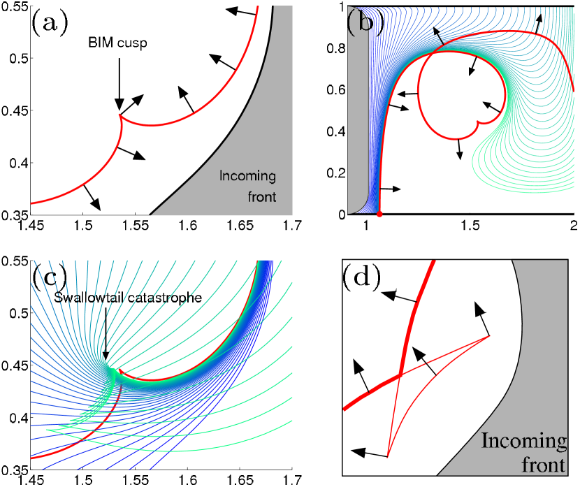
Figure 10: (color online) a) A BIM cusp. b) Zoom out of cusp with fronts wrapping around. c) Fronts spiraling and sliding past the cusp. d) A BIM with swallowtail structure.

The $xy$-projection of a BIM may form cusps, as seen in Figs. 1 and 2. A cusp in a BIM has a profound impact on the bounding nature of the BIM. This is because the burning direction (and hence bounding direction) of a BIM is reversed at a cusp, relative to an impinging front. See Fig. 10a. To the right of the cusp, the BIM is burning toward the upper left, acting as a barrier to the impinging front. However, left of the cusp, the BIM is burning toward the lower right. This flip in the burning direction results from the continuity of $\theta$ along the curve in the full $xy\theta$-space—note that the arrows in Fig. 10a rotate smoothly along the BIM. Thus, left of the cusp, the BIM does not act as a barrier to the front below; the front will simply pass through the left segment, as in Fig. 10c. Left of the cusp, the front spirals clockwise around the cusp and forms a swallowtail singularity. The front then slides past the cusp itself, moving toward the lower right and crossing over the right BIM segment from above. The critical observation is that the cusp provides an opening, through which the front can pass around the bounding segment of the BIM, and then collide with it. For time-independent flows, this is the only way for a front to reach the other side of a BIM.

Figure 10b shows a zoomed out view of the BIM and an initial front impinging from the left. Note that the evolving front passes right through the continuation of the BIM segment shown left of the cusp in Fig. 10a, owing to the orientation of its burning direction. However, although a cusp creates an opening in the bounding nature of a BIM, the entire remainder of the BIM is not necessarily irrelevant. Figure 10d shows an example of how a second cusp again reverses the burning direction ⁴⁷. Though the front may burn around each of the two cusps, the (bold) intervals still form a barrier to further front propagation.

IV.4 Moving past BIMs in time-periodic flows

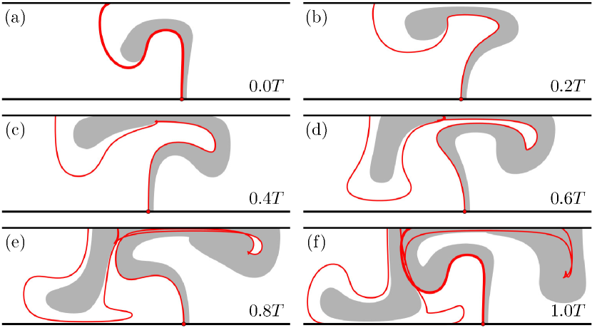
Figure 11: (color online) The mechanism by which a burned region (gray) may move past an initial BIM segment (red) under time-periodic driving.

For a time-periodic flow, a front may reach the other side of a BIM by a second mechanism illustrated in Fig. 11. Figure 11a shows an initial segment of a left-burning BIM (bold, red) that transects the fluid channel. A gray burned region is immediately right of the BIM. As the system evolves over one driving period, the BIM segment stretches and folds, ultimately crossing over itself (in the $xy$-projection). By the final frame, both the BIM and the front extend left of the original BIM segment (bold). While this may appear to violate the no-passing lemma, at no point does the burned region cross over any point of the BIM in the burning direction of the BIM. Furthermore, at each time step, the leftmost transecting segment of the BIM bounds the burned region. By the final frame, the burned region has moved past the original BIM segment because of the stretching and folding of the BIM itself. This mechanism is analogous to that of lobe dynamics (or turnstiles) for the advective transport of passive impurities in time-periodic flows ^{9; 11; 12; 48}.

IV.5 Convergence to BIMs and experimental measurement

Fronts are not only bounded by BIMs but converge upon them. This is due to the transverse stability of a BIM in the neighborhood of its SSU fixed point (a fact already utilized in Sec. IV.1). If a front has one front element that converges on a burning fixed point ⁴⁹, nearby front elements will evolve arbitrarily close to any given point of the BIM over time. This convergence is clearly witnessed in Figs. 1 and 2b, d.

Front convergence suggests a protocol to measure BIMs in the laboratory. For the time-independent case, first catalyze a reaction front sufficiently near the burning fixed point. (The advective fixed point is often a good choice.) Then observe the limiting behavior of the evolving front, which identifies the BIM location, as simulated in Fig. 1a. Points on the BIM nearest the fixed point will approach their limiting value earlier than points further along the BIM, and hence can be measured with greater accuracy ⁵⁰. This protocol has been successfully implemented in the Solomon lab, as discussed in the companion article ²⁰ and Ref. (18).

For the time-periodic case, a similar protocol exists, with one critical change. Care must be taken to record the converging front at a constant phase of the driving (say $t=0$). Hence, multiple experimental runs are needed in which the reaction is stimulated at incrementally earlier times $t<0$, and then recorded at the common time $t=0$. See Ref. (18) for further details and an experimental implementation.

BIMs can also be computed directly from the dynamics Eq. (5) if the flow $\mathbf{u}(\mathbf{r},t)$ is known. However, the ability to measure BIMs directly in experimental flows frees one from the requirement of either theoretically modeling $\mathbf{u}(\mathbf{r},t)$ or experimentally measuring $\mathbf{u}(\mathbf{r},t)$, e.g. from particle-tracking data.

As a front is converging upon a given point $\mathbf{r}$ of a BIM, another interval of the front may have taken a different route to collide with the BIM at $\mathbf{r}$ from the other side (as discussed in Sects. IV.3 and IV.4). Once this happens, one can no longer image the convergence upon $\mathbf{r}$, since the entire neighborhood of $\mathbf{r}$ is burned. Thus, the accuracy by which the BIM can be measured is limited by the time it takes another interval of the front to collide with the BIM. The best strategy then is to initialize the front as close to the burning fixed point as possible, allowing the most time to approach any given point on the BIM before the convergence process is wiped out. An enhanced strategy, permitting a more detailed measurement of the BIMs, would be to also suppress, or “erase”, the second front before it collides with the point $\mathbf{r}$ being measured. This could be done optically for certain photosensitive reactions.

Front Propagation Effects

1. Growth in the total area of the impurity region

2. Formation of cusps, swallowtails, and self-intersections at the impurity boundary (and within a BIM)

3. Directionality (i.e. existence of a burning direction) for the impurity boundary (and for a BIM)

Advection Effects

1. Existence of fixed points and invariant manifolds (BIMs)

2. Bounding property of invariant manifolds and use in transport

3. Convergence of impurity boundary to invariant manifolds

4. Lobe dynamics approach to transport of impurity region

Table 2: Comparison of front versus advection effects

V Concluding Remarks

A useful framework for organizing the properties of front propagation in a flowing medium [Eq. (4)] is to consider the two natural limiting cases: $\mathbf{u}=0$ (front propagation in a stationary medium) and $v_{0}=0$ (passive advection). In both limits, one is concerned with the change in geometry of an “impurity” region (either passive tracers or an active chemical medium) within a “background” medium. The front dynamics, and the BIMs in particular, reflect properties unique to one limit or the other, as summarized in Table 2. For example, the formation of cusps in a BIM reflects behavior typical in front propagation, but does not occur for invariant manifolds used in advection. Similarly, BIMs have a burning direction, which is natural for fronts, but absent for advective manifolds. On the other hand, the very existence of BIMs, their use as bounding curves, and their application to transport reflect similarities with the advection problem but are absent from studies of front propagation in homogeneous stationary media.

Appendix A Derivations

A.1 Derivation of Eq. (28)

The (signed) curvature of a planar curve $\mathcal{C}$ equals

$$\kappa=\mathbf{e}_{2}^{\prime}\cdot\frac{d\mathbf{e}_{1}^{\prime}}{d\lambda},$$ (48)

where $\mathbf{e}_{1}^{\prime}$ and $\mathbf{e}_{2}^{\prime}$ are the normal and tangent unit vectors to the curve, as in Sec. III.3. (Here, $\kappa<0$ implies $\mathbf{e}_{1}^{\prime}$ points toward the center of curvature.) We denote $\mathsf{R}(\lambda)$ as the rotation matrix connecting the $(\mathbf{e}_{1}^{\prime},\mathbf{e}_{2}^{\prime})$ frame to the laboratory frame $(\mathbf{e}_{1},\mathbf{e}_{2})=(\mathbf{\hat{x}},\mathbf{\hat{y}})$, i.e.

$$\mathbf{e}_{i}^{\prime}(\lambda)=\mathsf{R}(\lambda)\mathbf{e}_{i},\;i=1,2.$$ (49)

The components of a vector then transform using $\mathsf{R}^{T}$, e.g.

$$\mathbf{u}^{\prime}(\lambda)=\mathsf{R}^{T}(\lambda)\mathbf{u}(\lambda).$$ (50)

Specializing to a burning fixed point, at which $\mathbf{n}=\mathbf{e}_{1}^{\prime}$ and $\mathbf{g}=\mathbf{e}_{2}^{\prime}$ (Theorem 2), Eqs. (48) and (49) yield

$$\kappa=\mathbf{e}_{2}^{\prime}\cdot\frac{d\mathsf{R}}{d\lambda}\mathsf{R}^{T}\mathbf{e}_{1}^{\prime}=\mathbf{g}\cdot\frac{d\mathsf{R}}{d\lambda}\mathsf{R}^{T}\mathbf{n}.$$ (51)

From $d\mathbf{u}/d\lambda=\mu\mathbf{g}$, we then have

$$\mu =\mathbf{g}\cdot\frac{d\mathbf{u}}{d\lambda}=\mathbf{g}\cdot\left[\frac{d\mathsf{R}}{d\lambda}\mathsf{R}^{T}\mathbf{u}+\mathsf{R}\frac{d\mathbf{u}^{\prime}}{d\lambda}\right]$$

$$=\mathbf{g}\cdot\left[-v_{0}\frac{d\mathsf{R}}{d\lambda}\mathsf{R}^{T}\mathbf{n}+\mu^{\prime}\mathsf{R}\mathbf{g}^{\prime}\right]=-v_{0}\kappa+\mu^{\prime},$$ (52)

where the second equality follows from Eq. (50), the third from Eqs. (11) and (27), and the last from Eqs. (51) and the fact $\mathbf{g}=\mathsf{R}\mathbf{g}^{\prime}$. This yields Eq. (28).

A.2 Derivation of Eq. (29)

The (signed) curvature of the level set $f(\mathbf{r})=0$ for a general function $f$ is

$$\kappa=\frac{\mathbf{e}_{2}^{\prime}\cdot(\nabla\nabla f)\mathbf{e}_{2}^{\prime}}{\nabla f\cdot\mathbf{e}_{1}^{\prime}}.$$ (53)

Taking $f=|\mathbf{u}|^{2}-v_{0}^{2}$ defines the level set $\mathcal{C}$. Since $\mathbf{e}_{1}^{\prime}=\mathbf{n}$ and $\mathbf{e}_{2}^{\prime}=\mathbf{g}$ at a burning fixed point, the denominator of Eq. (53) becomes

$$(\nabla|\mathbf{u}|^{2})\cdot\mathbf{n} =-2v_{0}\mathbf{n}\cdot(\nabla\mathbf{u})\mathbf{n}$$

$$=-2v_{0}(\mbox{Tr}(\nabla\mathbf{u})-\mathbf{g}\cdot(\nabla\mathbf{u})\mathbf{g})=-2v_{0}\nu,$$ (54)

where the first equality follows from Eq. (11) and the final equality from Eq. (13) and the fact that $\mbox{Tr}(\nabla\mathbf{u})=\mu+\nu$. Similarly, a straightforward application of Eqs. (11) and (13) reveals the numerator of Eq. (53) to be

$$\mathbf{g}\cdot(\nabla\nabla|\mathbf{u}|^{2})\mathbf{g}=2\mu^{2}-2v_{0}\mathbf{a}\cdot\mathbf{g}.$$ (55)

Eq. (29) then follows from Eqs. (53) – (55).

References

- Bayfield and Koch (1974) J. E. Bayfield and P. M. Koch, “Multiphoton ionization of highly excited hydrogen atoms,” Phys. Rev. Lett., 33, 258–261 (1974).
- Koch and van Leeuwen (1995) P. M. Koch and K. A. H. van Leeuwen, “The importance of resonances in microwave ‘ionization’ of excited hydrogen atoms,” Phys. Rep., 255, 289 – 403 (1995).
- Mitchell et al. (2004) K. A. Mitchell, J. P. Handley, B. Tighe, A. Flower, and J. B. Delos, “Chaos-induced pulse trains in the ionization of hydrogen,” Phys. Rev. Lett., 92, 073001 (2004a).
- Mitchell et al. (2004) K. A. Mitchell, J. P. Handley, B. Tighe, A. Flower, and J. B. Delos, “Analysis of chaos-induced pulse trains in the ionization of hydrogen,” Phys. Rev. A, 70, 043407 (2004b).
- Burke and Mitchell (2009) K. Burke and K. A. Mitchell, “Chaotic ionization of a rydberg atom subjected to alternating kicks: Role of phase-space turnstiles,” Phys. Rev. A, 80, 033416 (2009).
- Burke et al. (2011) K. Burke, K. A. Mitchell, B. Wyker, S. Ye, and F. B. Dunning, “Demonstration of turnstiles as a chaotic ionization mechanism in rydberg atoms,” Phys. Rev. Lett., 107, 113002 (2011).
- Blümel and Reinhardt (1997) R. Blümel and W. P. Reinhardt, Chaos in atomic physics (Cambridge University Press, Cambridge, United Kingdom, 1997).
- Jaffé et al. (2002) C. Jaffé, S. D. Ross, M. W. Lo, J. Marsden, D. Farrelly, and T. Uzer, “Statistical theory of asteroid escape rates,” Phys. Rev. Lett., 89, 011101 (2002).
- MacKay et al. (1984) R. S. MacKay, J. D. Meiss, and I. C. Percival, “Transport in hamiltonian systems,” Physica D, 13, 55 (1984).
- Ottino (1989) J. M. Ottino, The kinematics of mixing: stretching, chaos, and transport (Cambridge University Press, United Kingdom, 1989).
- Rom-Kedar and Wiggins (1990) V. Rom-Kedar and S. Wiggins, “Transport in two-dimensional maps,” Archive for Rational Mechanics and Analysis, 109, 239 (1990).
- Wiggins (1992) S. Wiggins, Chaotic Transport in Dynamical Systems (Springer-Verlag, New York, 1992).
- Tel et al. (2005) T. Tel, A. de Moura, C. Grebogi, and G. Karolyi, “Chemical and biological activity in open flows: A dynamical system approach,” Phys. Rep., 413, 91–196 (2005).
- John and Mezic (2007) T. John and I. Mezic, “Maximizing mixing and alignment of orientable particles for reaction enhancement,” Phys. Fluids, 19 (2007).
- Neufeld and Hernandez-Garcia (2009) Z. Neufeld and E. Hernandez-Garcia, Chemical and Biological Processes in Fluid Flows: A Dynamical Systems Approach (Imperial College Press, 2009).
- Scotti and Pineda (2007) A. Scotti and J. Pineda, J. Marine Res., 65, 117–145 (2007).
- Sandulescu et al. (2008) M. Sandulescu, C. Lopez, E. Hernandez-Garcia, and U. Feudel, “Biological activity in the wake of an island close to a coastal upwelling,” Ecological Complexity, 5, 228–237 (2008).
- Mahoney et al. (2012) J. Mahoney, D. Bargteil, M. Kingsbury, K. Mitchell, and T. Solomon, “Invariant barriers to reactive front propagation in fluid flows,” submitted to Euro. Phys. Lett. (2012).
- Boehmer and Solomon (2008) J. R. Boehmer and T. H. Solomon, “Fronts and trigger wave patterns in an array of oscillating vortices,” Euro. Phys. Lett., 83, 58002 (2008).
- Bargteil and Solomon (2012) D. Bargteil and T. Solomon, “Barriers to front propagation in ordered and disordered vortex flows,” submitted to Chaos (2012).
- Note (1) Throughout, we use the term “burned” or “burning” generically for front propagation.
- Paoletti and Solomon (2005) M. S. Paoletti and T. H. Solomon, “Experimental studies of front propagation and mode-locking in an advection-reaction-diffusion system,” Euro. Phys. Lett., 69, 819 (2005a).
- Paoletti and Solomon (2005) M. S. Paoletti and T. H. Solomon, “Front propagation and mode-locking in an advection-reaction-diffusion system,” Phys. Rev. E, 72, 046204 (2005b).
- Paoletti et al. (2006) M. S. Paoletti, C. R. Nugent, and T. H. Solomon, “Synchronization of oscillating reactions in an extended fluid system,” Phys. Rev. Lett., 96, 124101 (2006).
- Schwartz and Solomon (2008) M. E. Schwartz and T. H. Solomon, “Chemical reaction fronts in ordered and disordered cellular flows with opposing winds,” Phys. Rev. Lett., 100, 028302 (2008).
- Pocheau and Harambat (2006) A. Pocheau and F. Harambat, “Effective front propagation in steady cellular flows: A least time criterion,” Phys. Rev. E, 73, 065304 (2006).
- Pocheau and Harambat (2008) A. Pocheau and F. Harambat, “Front propagation in a laminar cellular flow: Shapes, velocities, and least time criterion,” Phys. Rev. E, 77, 036304 (2008).
- Embid et al. (1995) P. F. Embid, A. J. Majda, and P. E. Souganidis, “Comparison of turbulent flame speeds from complete averaging and the g-equation,” Phys. Fluids, 7, 2052–2060 (1995), ISSN 10706631.
- Haller (2000) G. Haller, “Finding finite-time invariant manifolds in two-dimensional velocity fields,” Chaos, 10, 99–108 (2000), ISSN 10541500.
- Haller and Yuan (2000) G. Haller and G. Yuan, “Lagrangian coherent structures and mixing in two-dimensional turbulence,” Physica D, 147, 352 – 370 (2000), ISSN 0167-2789.
- G. and Haller (2001) G. and Haller, “Distinguished material surfaces and coherent structures in three-dimensional fluid flows,” Physica D, 149, 248 – 277 (2001), ISSN 0167-2789.
- Haller (2002) G. Haller, “Lagrangian coherent structures from approximate velocity data,” Phys. Fluids, 14, 1851–1861 (2002), ISSN 10706631.
- Shadden et al. (2005) S. C. Shadden, F. Lekien, and J. E. Marsden, “Definition and properties of lagrangian coherent structures from finite-time lyapunov exponents in two-dimensional aperiodic flows,” Physica D, 212, 271 – 304 (2005), ISSN 0167-2789.
- Shadden et al. (2006) S. C. Shadden, J. O. Dabiri, and J. E. Marsden, “Lagrangian analysis of fluid transport in empirical vortex ring flows,” Physics of Fluids, 18, 047105 (2006).
- Oberlack and Cheviakov (2010) M. Oberlack and A. F. Cheviakov, “Higher-order symmetries and conservation laws of the g-equation for premixed combustion and resulting numerical schemes,” J. Eng. Math., 66, 121–140 (2010).
- Solomon and Gollub (1988) T. H. Solomon and J. P. Gollub, “Chaotic particle transport in time-dependent Rayleigh-Bénard convection,” Phys. Rev. A, 38, 6280–6286 (1988).
- Camassa and Wiggins (1991) R. Camassa and S. Wiggins, “Chaotic advection in a rayleigh-bénard flow,” Phys. Rev. A, 43, 774–797 (1991).
- Cencini et al. (2003) M. Cencini, A. Torcini, D. Vergni, and A. Vulpiani, “Thin front propagation in steady and unsteady cellular flows,” Phys. Fluids, 15, 679–688 (2003), ISSN 10706631.
- Note (2) Channel walls that restrict the fluid domain may also be included in the model, as in Figs. 1 and 2. In this case, the velocity of a front element need not be tangent to the wall, though certainly must be. Instead, a front element can collide with the wall, after which it ceases to be physically relevant. Theoretically, it can be useful to keep track of such front elements by freezing them in place on the boundary. (Numerically, a narrow boundary layer is used to slow the speed of the front elements to zero.) Keeping track of these points avoids clipping the front and permits one to determine how all of the front segments within the fluid are connected.
- You et al. (1991) Z. You, E. J. Kostelich, and J. A. Yorke, “Calculating stable and unstable manifolds,” Int. J. Bifurcation Chaos, 1, 605–623 (1991).
- Abel et al. (2001) M. Abel, A. Celani, D. Vergni, and A. Vulpiani, “Front propagation in laminar flows,” Phys. Rev. E, 64, 046307 (2001).
- Abel et al. (2002) M. Abel, M. Cencini, D. Vergni, and A. Vulpiani, “Front speed enhancement in cellular flows,” Chaos, 12, 481–488 (2002), ISSN 10541500.
- Arnold (1983) V. I. Arnold, Catastrophe Theory (Springer, Berlin, 1983).
- Arnold (1989) V. I. Arnold, Mathematical Methods of Classical Mechanics (Springer, New York, NY, 1989).
- Guckenheimer and Holmes (1983) J. Guckenheimer and P. Holmes, Nonlinear oscillations, dynamical systems, and bifurcations of vector fields (Springer, New York, 1983).
- Note (3) If the original segment were to lie exactly within the two-dimensional stable manifold of the fixed point, the segment would converge to the fixed point only. In this case, the original segment could be perturbed slightly out of the stable manifold everywhere except the fixed point, while still preserving Eq. (6).
- Note (4) The geometry of Fig. 10d can only happen in the time-periodic case. In the time-independent case, it is forbidden because: (i) the BIM consists of a single trajectory and (ii) this trajectory would violate the no-passing lemma if it were to pass through the intersection point of the swallowtail in Fig. 10d.
- Solomon et al. (1996) T. H. Solomon, S. Tomas, and J. L. Warner, “Role of lobes in chaotic mixing of miscible and immiscible impurities,” Phys. Rev. Lett., 77, 2682–2685 (1996).
- Note (5) Equivalently, we may consider any front that intersects the stable manifold of the fixed point, or alternatively, any front for which the stable manifold passes through the burned region.
- Note (6) This ignores long-time experimental effects, such as flow inconsistencies or Ekman pumping 51.
- Solomon and Mezić (2003) T. H. Solomon and I. Mezić, “Uniform resonant chaotic mixing in fluid flows,” Nature, 425, 376 (2003).