OHSTPY-HEP-T-12-001

SU(6) GUT Breaking on a Projective Plane

Archana Anandakrishnan, Stuart Raby

Department of Physics, The Ohio State University,

191 W. Woodruff Ave, Columbus, OH 43210, USA

Abstract

We consider a 6-dimensional supersymmetric SU(6) gauge theory and compactify two extra-dimensions on a multiply-connected manifold with non-trivial topology. The SU(6) is broken down to the Standard Model gauge groups in two steps by an orbifold projection (or Wilson line), followed by a Wilson line. The Higgs doublets of the low energy electroweak theory come from a chiral adjoint of SU(6). We thus have gauge-Higgs unification. The three families of the Standard Model can either be located in the 6D bulk or at 4D N=1 supersymmetric fixed points.

We calculate the Kaluza-Klein spectrum of states arising as a result of the orbifolding. We also calculate the threshold corrections to the coupling constants due to this tower of states at the lowest compactification scale. We study the regions of parameter space of this model where the threshold corrections are consistent with low energy physics. We find that the couplings receive only logarithmic corrections at all scales. This feature can be attributed to the large N=2 6D SUSY of the underlying model.

1 Introduction

A supersymmetric grand unified description[1, 2, 3, 4, 5, 6] of the fundamental forces of nature has been the holy grail of particle physics for many years now. Such a unified description would bring some order into the chaotic world of particle representations. In addition, the many different parameters of the Standard Model can be tied down using a grand unified symmetry. Unfortunately, most such unified descriptions in 4-dimensions are haunted by many issues. Two notable problems with 4-dimensional supersymmetric grand unified theories (SUSY GUTs) include the Higgs doublet-triplet splitting problem and the complicated potentials required to break the grand unified symmetry down to the Standard Model gauge groups. Apart from these theoretical hindrances, the major setback to 4D SUSY GUTs came with the experimental non-observation of proton decay at the predicted life-times of the models[7, 8]. SuperK places the current lower bound on the proton lifetime ($p\rightarrow e^{+}\pi^{0}$) to be 1 $\times\ 10^{34}$ years[9]. Also, SUSY GUTs, with the standard CMSSM scenario of SUSY breaking, require GUT-scale threshold corrections of about $-$3% in order to fit the low energy value of the strong coupling.

An elegant and definitive solution to the above stated theoretical issues was proposed in models of orbifold GUTs. Grand unified theories constructed in higher dimensional spaces could be reduced to 4-dimensional GUTs by compactifying the extra-dimensions on specific manifolds[10, 11]. By doing so, it was found that the Higgs doublet-triplet problem could be solved in a simple manner by choosing the correct parities along the strong and the weak directions[12, 13]. Many orbifold GUTs have been constructed since then[15, 14, 16, 17, 18, 19, 20], with interesting phenomenology and realistic supersymmetric spectrum. The Kaluza-Klein tower of states that arise in these extra-dimensional GUTs can also account for the GUT scale threshold corrections[13, 19, 20, 21, 22]. It must be pointed out that orbifold GUT model-building in field theory constructions mirrored the earlier work in heterotic string theory constructions[23, 24, 25, 26]. In recent years, many different features of orbifold compactifications have been studied both from a phenomenological bottom-up approach, as well as top-down from string theory. Within the context of string theory, gauge coupling unification occurs at the string scale. This may occur with or without an intermediate GUT. However, such theories have the problem that the string scale is typically about 20 times larger than the 4D GUT scale [27, 28, 29]. One might hope that gauge coupling unification can be reconciled with string unification by lowering the string unification scale. It has been argued that non-local breaking of the GUT symmetry via Wilson lines on an anisotropic orbifold can solve the problem of string unification [32, 30, 31]. In this paper we provide a self-consistent test of this hypothesis on a particular 6D orbifold. It is possible that this orbifold GUT is an effective low energy theory of some string compactification, but we have not come across any compactification that would lead to an orbifold with the topology discussed here.

In this work, we present a 6D model with SU(6) gauge symmetry and N=2 supersymmetry. In terms of 4D language, such a 6D theory with N=2 SUSY contains one vector adjoint and three chiral adjoints. The model has gauge-Higgs unification with the Higgs doublets coming from one of the chiral adjoints. The group SU(6) is broken to SU(5) $\times$ U(1)_X via orbifold boundary conditions. Then SU(5) is broken to the Standard Model gauge group and, at the same time, Higgs doublet-triplet splitting is accomplished by a non-local Wilson line. The two extra-dimensions are compactified on an orbifold that can be characterized as a sphere with a cross-cap, as described in [33, 30, 31]. Quarks and leptons, and their respective Yukawa couplings to the Higgs, are localized at the orbifold fixed points which only retain an N=1 SUSY in 4D with SU(5) $\times$ U(1)_X gauge invariance (see for example Refs. [13, 17] where this phenomenon has been discussed).

The details of the orbifold and the symmetry breaking are discussed in Section 2. We break the SU(6) $\rightarrow$ SU(5) $\times$ U(1)_X using one of the orbifold projections, locally at the fixed points. We then break the SU(5) $\rightarrow$ SU(3) $\times$ SU(2) $\times$ U(1)_Y using a Wilson line along the fifth and sixth directions. In Section 3, we analyze gauge coupling unification in the SU(6) GUT model constructed on such an orbifold and calculate the GUT-scale threshold corrections in this scenario. We find that unlike in most popular models of orbifold GUTs, the couplings do not receive any power law corrections above the compactification scale due to the effective N=4 SUSY in 4D. We analyze the GUT-scale threshold corrections to determine if they are at the required level to match low energy physics. We point out that an example of an orbifold GUT from a 6D SU(6) was considered in[17] with the the similar feature of gauge-Higgs unification. The extra-dimensions were compactified on $T^{2}/(Z_{2}\times Z^{\prime}_{2})$ and the authors obtain realistic phenomenology with local GUT breaking. The 6D GUT theory also had an N=2 supersymmetry. As a consequence, the coefficient of the effective 6D quadratic power law dependence of the gauge couplings vanished, but due to the existence of fixed lines the effective 5D linear dependence remained.

2 GUT breaking

2.1 Real Projective Plane

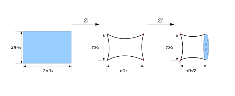
An N=2 supersymmetric SU(6) gauge theory in 6 dimensions is compactified on an orbifold, shown in Fig 1, as described in Hebecker[33]. The extra dimensions are compactified on a torus $T^{2}$ parametrized by ($x_{5}$, $x_{6}$). The two dimensions are also identified to have the periodicity, $x_{(5,6)}=x_{(5,6)}+2\pi R_{(5,6)}$, where $R_{5}$ and $R_{6}$ are the radius of the torus along the two directions. Two discrete symmetries, the rotation ${\cal Z}$ and a freely acting roto-translation ${\cal Z}^{\prime}$, as defined in Eq.(1, 2) are modded out. Once the first symmetry is modded out, the topology of the compact space is that of a 2-sphere with curvature concentrated at the four conical singularities. The space resembles a pillow with fundamental group $\pi_{1}=\emptyset$. Once the second parity is modded out, the resulting compact space is equivalent to a projective plane, $RP^{2}$. It is non-orientable with no boundaries, the curvature is concentrated at the two fixed points denoted by $F_{1}$ and $F_{2}$ and $\pi_{1}={\mathbb{Z}}_{2}$. The non-orientability of the space can be ascribed to the cross-cap where opposite points on the circle are identified.

$${\cal Z} x_{5}\rightarrow-x_{5}, x_{6}\rightarrow-x_{6}$$ (1)

$${\cal Z}^{\prime} x_{5}\rightarrow-x_{5}+\pi R_{5}, x_{6}\rightarrow x_{6}+\pi R_{6}.$$ (2)

Figure 1: The figure shows the manifold at each step of the compactification. After the first step of orbifolding, the space looks like a pillow with four fixed points denoted by red dots in the center figure. After the second step of orbifolding as described in [33], this space is equivalent to a real projective plane.

We choose to write the particle content of the theory in terms of the 4D language. There is one vector superfield, V and three chiral superfields, $\Sigma_{5}$, $\Sigma_{6}$, and $\Phi$. Using the notation in [17], the bulk action in the Wess-Zumino gauge is given by:

$$S = \int d^{6}x\Biggl{\{}{\rm Tr}\Biggl{[}\int d^{2}\theta\Biggl{(}\frac{1}{4kg^{2}}{\cal W}^{\alpha}{\cal W}_{\alpha}$$ (3)

$$\qquad+\frac{1}{kg^{2}}\Bigl{(}\Phi\partial_{5}\Sigma_{6}-\Phi\partial_{6}\Sigma_{5}-\frac{1}{\sqrt{2}}\Phi[\Sigma_{5},\Sigma_{6}]\Bigr{)}\Biggr{)}+{\rm h.c.}\Biggr{]}$$

$$\qquad+\int d^{4}\theta\frac{1}{kg^{2}}{\rm Tr}\Biggl{[}(\sqrt{2}\partial_{5}+\Sigma_{5}^{\dagger})e^{-V}(-\sqrt{2}\partial_{5}+\Sigma_{5})e^{V}+$$

$$\qquad(\sqrt{2}\partial_{6}+\Sigma_{6}^{\dagger})e^{-V}(-\sqrt{2}\partial_{6}+\Sigma_{6})e^{V}$$

$$\qquad+\Phi^{\dagger}e^{-V}\Phi e^{V}+\partial_{5}e^{-V}\partial_{5}e^{V}+\partial_{6}e^{-V}\partial_{6}e^{V}\Biggr{]}\Biggr{\}}$$

2.2 SU(6) $\rightarrow$ SU(5) $\times$ U(1)_X

The 6D N=2 supersymmetric theory that we start with has an effective N=4 SUSY in 4 dimensions. The action of the above discussed parities can be used to break the gauge group SU(6) down to SU(5) $\times$ U(1)_X, and at the same time break N = 4 SUSY to N = 1 SUSY (in 4D) [34]. We can break SU(6) to SU(5) $\times$ U(1)_X by requiring the fields to transform as illustrated below, under the two parities.

Under the parity, ${\cal Z}$:

$$V(-x_{5},-x_{6}) = PV(x_{5},x_{6})P^{-1},$$

$$\Sigma_{5}(-x_{5},-x_{6}) = -P\Sigma_{5}(x_{5},x_{6})P^{-1},$$

$$\Sigma_{6}(-x_{5},-x_{6}) = -P\Sigma_{6}(x_{5},x_{6})P^{-1},$$

$$\Phi(-x_{5},-x_{6}) = P\Phi(x_{5},x_{6})P^{-1},$$ (4)

Under the parity, ${\cal Z^{\prime}}$:

$$V(-x_{5}+\pi R_{5},x_{6}+\pi R_{6}) = V(x_{5},x_{6}),$$

$$\Sigma_{5}(-x_{5}+\pi R_{5},x_{6}+\pi R_{6}) = -\Sigma_{5}(x_{5},x_{6}),$$

$$\Sigma_{6}(-x_{5}+\pi R_{5},x_{6}+\pi R_{6}) = \Sigma_{6}(x_{5},x_{6}),$$

$$\Phi(-x_{5}+\pi R_{5},x_{6}+\pi R_{6}) = -\Phi(x_{5},x_{6}).$$ (5)

where P = diag$(i,i,i,i,i,-i)$, breaks the SU(6) $\rightarrow$ SU(5) $\times$ U(1)_X. The projection ${\cal Z}$ has four fixed points(as shown in Fig 1) and hence the SU(6) symmetry is broken down to SU(5) $\times$ U(1)_X only at those fixed points. The symmetry breaking in this case is said to be localized. On the other hand, the second parity is freely acting (without any fixed points). Therefore, breaking the gauge symmetry using the second orbifold projection would have led to non-local breaking of the SU(6). It can be shown that the gauge symmetry breaking by this orbifold action can be rewritten as symmetry breaking by a Wilson line. However, as we shall see in the next section, we require an additional Wilson line to further break the SU(5) down to SU(3) $\times$ SU(2) $\times$ U(1)_Y. The conditions on the Wilson lines on this orbifold (to be discussed in the next section) do not allow for a minimal execution of the gauge symmetry breaking from SU(6) $\rightarrow$ SU(5) $\times$ U(1)_X $\rightarrow$ SU(3) $\times$ SU(2) $\times$ U(1)_Y $\times$ U(1)_X in a completely non-local way. Hence we choose to break the SU(6) $\rightarrow$ SU(5) $\times$ U(1)_X locally and the SU(5) non-locally using a Wilson line.

Under the combined operation (${\cal Z},{\cal Z}^{\prime}$) the components of the fields transform as follows:
$\displaystyle V=\left(\begin{array}[]{c|c|c}(++)(++)(++)&(++)(++)&(-+)\\ (++)(++)(++)&(++)(++)&(-+)\\ (++)(++)(++)&(++)(++)&(-+)\\ \hline\cr(++)(++)(++)&(++)(++)&(-+)\\ (++)(++)(++)&(++)(++)&(-+)\\ \hline\cr(-+)(-+)(-+)&(-+)(-+)&(++)\\ \end{array}\right)$ (12) $\displaystyle\Sigma_{5}=\left(\begin{array}[]{c|c|c}(--)(--)(--)&(--)(--)&(+-)\\ (--)(--)(--)&(--)(--)&(+-)\\ (--)(--)(--)&(--)(--)&(+-)\\ \hline\cr(--)(--)(--)&(--)(--)&(+-)\\ (--)(--)(--)&(--)(--)&(+-)\\ \hline\cr(+-)(+-)(+-)&(+-)(+-)&(--)\\ \end{array}\right)$ (19) $\displaystyle\Sigma_{6}=\left(\begin{array}[]{c|c|c}(-+)(-+)(-+)&(-+)(-+)&(++)\\ (-+)(-+)(-+)&(-+)(-+)&(++)\\ (-+)(-+)(-+)&(-+)(-+)&(++)\\ \hline\cr(-+)(-+)(-+)&(-+)(-+)&(++)\\ (-+)(-+)(-+)&(-+)(-+)&(++)\\ \hline\cr(++)(++)(++)&(++)(++)&(-+)\\ \end{array}\right)$ (26) $\displaystyle\Phi=\left(\begin{array}[]{c|c|c}(+-)(+-)(+-)&(+-)(+-)&(--)\\ (+-)(+-)(+-)&(+-)(+-)&(--)\\ (+-)(+-)(+-)&(+-)(+-)&(--)\\ \hline\cr(+-)(+-)(+-)&(+-)(+-)&(--)\\ (+-)(+-)(+-)&(+-)(+-)&(--)\\ \hline\cr(--)(--)(--)&(--)(--)&(+-)\\ \end{array}\right)$ (33)

The parity operations (${\cal Z},{\cal Z}^{\prime}$) performed on the coordinate space are symmetries of the Lagrangian, hence the fields in the Lagrangian must be eigenstates of the parity operations. A general field $\varphi=\{V,\Sigma_{5},\Sigma_{6},\Phi\}$ by definition of the manifold, are periodic functions of $x_{5}$ and $x_{6}$.

$$\varphi(x,x_{5}+2\pi R_{5},x_{6})=\varphi(x,x_{5},x_{6})$$

$$\varphi(x,x_{5},x_{6}+2\pi R_{6})=\varphi(x,x_{5},x_{6})$$ (35)

This allows us to expand them as:

$$\varphi(x,x_{5},x_{6})=\frac{1}{\sqrt{2\pi R_{5}R_{6}}}\sum_{m,n=-\infty}^{+\infty}\varphi^{(m,n)}\text{exp}\left[i\left(\frac{mx_{5}}{R_{5}}+\frac{nx_{6}}{R_{6}}\right)\right]\\$$ (36)

The eigenstates of the parity operations are required to obey:

$$\varphi_{\pm\widehat{\pm}}(x_{\mu},-x_{5},-x_{6}) = \pm\varphi_{\pm\widehat{\pm}}(x_{\mu},x_{5},x_{6})$$

$$\varphi_{\pm\widehat{\pm}}(x_{\mu},-x_{5}+\pi R_{5},x_{6}+\pi R_{6}) = \widehat{\pm}\varphi_{\pm\widehat{\pm}}(x_{\mu},x_{5},x_{6})$$ (37)

which project out even and odd modes that can be written out as:

$$\varphi_{\pm\widehat{\pm}}(x,x_{5},x_{6})=\frac{1}{4\sqrt{2\pi R_{5}R_{6}}}$$

$$\times\sum_{m,n}\left[(\varphi^{(m,n)}\pm\varphi^{(-m,-n)})\widehat{\pm}(-1)^{m-n}(\varphi^{(-m,n)}\pm\varphi^{(m,-n)})\right]\text{exp}\left[i\left(\frac{mx_{5}}{R_{5}}+\frac{nx_{6}}{R_{6}}\right)\right]$$

(38)

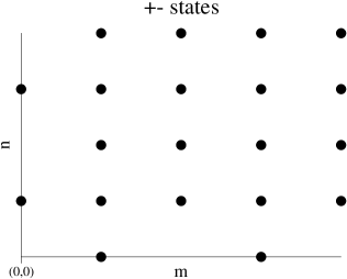
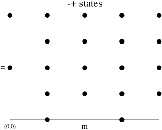
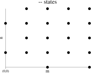
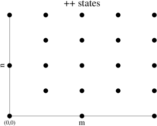
In the above three expressions, $\pm$ denotes states that are even/odd under the first parity operation, and $\widehat{\pm}$ denotes states that are even/odd under the second parity. The massless modes come only from the $+\widehat{+}$ (hereafter denoted as ++) parity modes. The above spectrum is illustrated in Fig. 2

Figure 2: The mode expansion in Eq.(38) gives the information about where the various parity eigenstates exist. Notice that this figure depicts only the positive parts of the (m,n) values while for the calculations they should be summed over both positive and negative integers. It is clear from the figure that only the $(++)$ fields have zero modes.

2.3 SU(5) $\rightarrow$ SU(3) $\times$ SU(2) $\times$ U(1)_Y

We now introduce a Wilson line to break the symmetry down to the Standard Model. A gauge field, $A_{M}\equiv\sum_{a}A_{M}^{a}T^{a}$ transforms under a gauge transformation as follows:

$$A_{M}(x_{\mu},x_{5},x_{6})\rightarrow UA_{M}(x_{\mu},x_{5},x_{6})U^{\dagger}-iU\partial_{M}U^{\dagger}$$ (39)

where $T^{a}$ correspond to the generators of the gauge group. Now consider a constant background gauge field along the fifth ans sixth directions:

$$A_{5}=\frac{1}{4R_{5}}T\quad\text{and},\quad A_{6}=\frac{1}{4R_{6}}T$$ (40)

where $T$ is the generator (up to a constant) that breaks SU(6) down to SU(3) $\times$ SU(3) $\times$ U(1) given by:

$$T=\left(\begin{array}[]{cccccc}1&&&&&\\ &1&&&&\\ &&1&&&\\ &&&-1&&\\ &&&&-1&\\ &&&&&-1\\ \end{array}\right)$$ (47)

Note that the choice of the background gauge fields must obey some strict constraints. For example, the space group generators obey:

$${\cal Z}^{2}=\mathds{1},\qquad{\cal Z^{\prime}}^{2}=T_{6}$$ (48)

The second condition implies that the action of the parity ${\cal Z^{\prime}}$ is equivalent to the holonomy coming from the gauge field along the sixth direction. In addition,

$${\cal ZZ^{\prime}ZZ^{\prime}}=T_{5}^{-1}$$ (49)

Rewriting the above relation of the space group generators as holonomies, we get:

$$G({\cal Z}^{2})G({\cal Z^{\prime}}^{2})=G(T_{5}^{-1})$$ (50)

where we have use the fact that U(1) holonomies commute. Noting that $G(T_{5}^{-1})$ = $G(T_{5})$, we find that the holonomies should obey the condition:

$$G(T_{5})=G(T_{6})$$ (51)

This statement tells us that the Wilson lines cannot be independent along the two extra-dimensions. The presence of such a background gauge field breaks the gauge symmetry. The constant background fields introduce a holonomy equal to $W=\text{exp}\left(i\oint A_{5}dx_{5}+i\oint A_{6}dx_{6}\right)$. This non-trivial holonomy affects the spectrum of Kaluza-Klein states. In an equivalent picture[35, 36], the background gauge field can be gauged away completely by choosing the proper gauge transformation, and in this case, we find that the gauge condensate vanishes when

$$U(x_{5})=\text{exp}\left[i\left(\frac{x_{5}}{R_{5}}+\frac{x_{6}}{R_{6}}\right)\frac{T}{4}\right]$$ (52)

Nevertheless, the physics remains unchanged, and we determine the change in the KK spectrum due to the non-trivial holonomy (or Wilson-line).

Under the gauge transformation operator, Eq.(52), a generic adjoint field $\varphi$ transforms as:

$$\varphi^{\prime}(x_{\mu},x_{5},x_{6})=U(x_{5},x_{6})\varphi(x_{\mu},x_{5},x_{6})U^{\dagger}(x_{5},x_{6})$$ (53)

which allows us to rewrite the gauge transformed wave function as

$$\varphi^{\prime}(x_{\mu},x_{5},x_{6})=\text{e}^{i\left(\frac{x_{5}}{R_{5}}+\frac{x_{6}}{R_{6}}\right)\frac{I_{\rho}}{4}}\varphi(x_{\mu},x_{5},x_{6})$$ (54)

where, $I_{\rho}$ is the eigenvalue of the generator T and $\varphi(x_{\mu},x_{5},x_{6})$ is the untransformed wave function as defined in Eq. (36). The periodicity condition Eq.(35) of the fields then becomes:

$$\varphi^{\prime}(x_{\mu},x_{5}+2\pi R_{5},x_{6}) = P^{\prime}\varphi^{\prime}(x_{\mu},x_{5},x_{6})P^{\prime\dagger}\equiv e^{i\frac{\pi}{2}I_{\rho}}\varphi^{\prime}(x_{\mu},x_{5},x_{6})$$

$$\varphi^{\prime}(x_{\mu},x_{5},x_{6}+2\pi R_{6}) = P^{\prime}\varphi^{\prime}(x_{\mu},x_{5},x_{6})P^{\prime\dagger}=e^{i\frac{\pi}{2}I_{\rho}}\varphi^{\prime}(x_{\mu},x_{5},x_{6})$$ (55)

where $P^{\prime}\equiv\text{exp}\left(i\frac{\pi}{2}T\right)=\text{diag}(i,i,i,-i,-i,-i)$. The above equation reflects the constraints on the Wilson lines that was demonstrated in Eq. (51). In addition, now we have re-expressed the Wilson line as a parity operation that breaks SU(6) down to SU(3) $\times$ SU(3) $\times$ U(1). Under the combined parity operations on the manifold and the non-vanishing background fields along the fifth and sixth directions, we have achieved gauge symmetry breaking of the SU(6) group to [SU(3) $\times$ SU(2) $\times$ U(1)_Y] $\times$ U(1)_X. The only choice we had here was a combination of local and non-local GUT breaking. It is possible to have a purely non local GUT breaking if one started with an SU(5) gauge theory on the same orbifold and and chose the second parity to break the SU(5) down to SU(3) $\times$ SU(2) $\times$ U(1) [33].

We still have to calculate how the mass spectrum changes as a result of the holonomy due to the gauge field. This can be easily done by looking at the transformed wave function in Eq.(54) and calculating the eigenvalues $I_{\rho}$ of the generator T. The eigenvalues $I_{\rho}$ can be determined by calculating the commutator $\left[T,\varphi\right]$ since $\varphi$ is in the adjoint representation, of the form:

$$\varphi= \left(\begin{array}[]{ccccc|ccc|c}&&&&&&&&\\ &&(8,1)_{0}&&&&(3,\bar{2})_{-5/3}&&(3,1)_{-2/3}\\ &&&&&&&&\\ \hline\cr&&&&&&&&\\ &&(\bar{3},2)_{5/3}&&&&(1,3)_{0}&&(1,2)_{1}\\ \hline\cr&&(\bar{3},1)_{2/3}&&&&(1,\bar{2})_{-1}&&(1,1)_{0}\\ \end{array}\right)$$ (62)

$$= \left(\begin{array}[]{ccccc|ccc|c}&&&&&&&&\\ &&g&&&&X&&T\\ &&&&&&&&\\ \hline\cr&&&&&&&&\\ &&\bar{X}&&&&w&&H_{u}\\ \hline\cr&&\bar{T}&&&&H_{d}&&b\\ \end{array}\right)$$ (69)

The first line in the above expression shows the quantum numbers of the the different blocks that the adjoint field gets broken into after the orbifold projection and holonomy. We name them appropriately, so that they can be associated with the fields that remain massless in the low energy theory, like the gauge bosons, $g,w,b$ and the Higgs doublets, $H_{u},H_{d}$; and the fields that obtain mass and do not appear in the low energy spectrum like the Higgs triplets $T,\bar{T}$ and states with exotic quantum numbers $X,\bar{X}$. The commutator of the generator $T$ with this quantity is calculated and the eigenvalues of are summarized in Table 1.

	$g$	$w$	$b$	$X$	$\bar{X}$	$T$	$\bar{T}$	$H_{u}$	$H_{d}$
$I_{\rho}$	0	0	0	2	-2	2	-2	0	0

Table 1: Eigenvalues $I_{\rho}$ of the generator T acting on the various fields (labelled by $\rho$) in the model.

Eventually, we see that the masses of the states in the KK tower are given by

$$M_{(m,n),\rho}^{2}=\frac{(m+\frac{I_{\rho}}{4})^{2}}{R_{5}^{2}}+\frac{(n+\frac{I_{\rho}}{4})^{2}}{R_{6}^{2}}$$ (70)

The massless states are those which are even under both parities and have zero eigenvalue under the holonomy. These turn out to be only the standard model gauge bosons and the Higgs doublets, $H_{u},H_{d}$ coming from the chiral adjoint $\Sigma_{6}$. Finally, we also note that at the two fixed points, $F_{1}$ and $F_{2}$ which are located at $(0,0)$ and $(0,\pi R_{6})$, there is only an SU(5) whereas the bulk has an SU(6). The three families of quarks and leptons are also assumed to sit at these singularities coming in 3 ($\bf 10_{F}+\bar{5}_{F}$) representations. The Yukawa couplings are also assumed to be localized at these fixed points. They require superpotential terms of the form $\bf 10_{F}\ 10_{F}\ 5_{\Sigma_{6}}+10_{F}\ \bar{5}_{F}\ \bar{5}_{\Sigma_{6}}$ where the indices are contracted in an obvious way. The SU(5) relation $\lambda_{b}=\lambda_{\tau}$ works for the third family but not for the first two. It is possible that interaction with matter in the bulk could help with this issue, but this is beyond the scope of this paper.

2.4 Proton decay

Dimension 6 operators for proton decay are suppressed by the inverse power squared of the smallest compactification scale. We will see that this is near the 4D GUT scale and thus the proton lifetime is completely consistent with the experimental bounds. On the other hand, dimension 5 operators for proton decay are only suppressed by the inverse power of the compactification scale. However, if we assume that quarks and leptons only couple to the chiral adjoints containing the Higgs fields, there are no dimension 5 operators for proton decay generated when integrating out the color triplet Higgs fields. This can be attributed to an unbroken $\mathbb{Z}_{4}^{R}$ symmetry [40] where the superpotential has charge 2, families have charge 1, $\{\Sigma_{5,6},\ 6,\ \bar{6}\}$ have charge 0, and $\{S,\ \Phi\}$ have charge 2.

3 Threshold Corrections

4D SUSY GUTs require extra states to contribute a small amount of threshold corrections at the GUT scale in order to concur with low energy measurements. Conventionally, this quantity of GUT scale threshold corrections (defined at the 4D GUT scale) is defined as:

$$\epsilon_{3}=\frac{\alpha_{3}-\alpha_{GUT}}{\alpha_{GUT}}.$$ (71)

The running coupling constants in the 4D MSSM can be summarized by:

$$\alpha_{i}^{-1}(Q)=\alpha_{GUT}^{-1}+\frac{b_{i}}{2\pi}log\frac{M_{GUT}}{Q}-\alpha_{GUT}^{-1}\frac{\epsilon_{3}}{(1+\epsilon_{3})}\delta_{i3}$$ (72)

where $\delta_{i3}$ denotes that the term appears only for i=3 (the coupling $\alpha_{3}$). The exact amount of threshold corrections required from the extra states is usually model dependent, but they have to be around a few percent level. For the most popular scenarios of MSSM with unified gaugino masses, this number turns out to be about -3%. We would like to calculate the effect of the Kaluza-Klein (KK) tower of infinite states to the running of coupling constants in the orbifold model that we have just constructed. These additional contributions to the running of the coupling constants from KK modes can be written as:

$$\frac{4\pi}{g_{i}^{2}(\mu)}=\frac{4\pi}{g^{2}(\Lambda)}+\sum_{\rho}\Omega_{i,\rho}(\mu)$$ (73)

where

$$\Omega_{i,\rho}(\mu)\equiv\frac{1}{4\pi}\sum_{(m,n)\in Z}\beta_{i,\rho}\int_{\xi}^{\infty}\frac{dt}{t}e^{-\pi t\frac{M_{(m,n),\rho}^{2}}{\mu^{2}}}e^{-\pi\chi t}$$ (74)

includes one-loop corrections from both massive and massless states in the theory. $\xi$ is the ultraviolet (UV) regulator introduced since the integral is UV-divergent. $\chi$ is an infrared (IR) regulator introduced since the above quantity diverges for the special case when there are massless states in the KK tower. The corrections come from each state $\rho$ that appears in the spectrum, with an associated beta-function coefficient, $\beta_{i,\rho}$, summarized in Table 2 and mass, $M_{(m,n),\rho}^{2}$, as calculated in the previous section:

$$M_{(m,n),\rho}^{2}=\frac{(m+\frac{I_{\rho}}{4})^{2}}{R_{5}^{2}}+\frac{(n+\frac{I_{\rho}}{4})^{2}}{R_{6}^{2}}$$ (75)

We evaluate the expression in Eq. (74) in three different regions on the m-n plane shown in Fig 2 and then sum up the contributions to find the total corrections to the couplings.

3.1 States at m = 0 and n = 0

In this case, the contribution to the threshold corrections is:

$$\Omega_{i,\rho}^{00}(\mu)=\frac{1}{4\pi}\beta_{i,\rho}\int_{\xi}^{\infty}\frac{dt}{t}e^{-\pi t\frac{M_{(0,0),\rho}^{2}}{\mu^{2}}}e^{-\pi\chi t}$$ (76)

We saw earlier that the only states at the m=0, n=0 point are the (++) modes. The (++) modes come from the N=1 SUSY vector fields $g,w,b,X,\bar{X},$ and chiral adjoint fields $T,\bar{T},H_{u},H_{d}$. The beta-function coefficients for these states are summarized in Table 2. Using the results from Appendix, we find:

$$\Omega_{i}^{00}=\frac{b^{++}_{i}(I_{\rho}=0)}{4\pi}\Gamma\left[0,\pi\xi\chi\right]+\frac{b^{++}_{i}(I_{\rho}=2)}{4\pi}\Gamma\left[0,\pi\xi\left(\frac{1}{4\mu^{2}R_{5}^{2}}+\frac{1}{4\mu^{2}R_{6}^{2}}+\chi\right)\right]$$ (77)

Quantum Number	Name	Type	$b_{1}$	$b_{2}$	$b_{3}$	Type	$b_{1}$	$b_{2}$	$b_{3}$
(8,1)0	$g$	C	0	0	3	V	0	0	-9
(1,3)0	$w$	C	0	2	0	V	0	-6	0
(3,2)±5/3	$X,\bar{X}$	C	5/2	3/2	1	V	-15/2	-9/2	-3
(3,1)±2/3	$T,\bar{T}$	C	1/5	0	1/2	V	-3/5	0	-3/2
(1,2)±1	$H_{u},H_{d}$	C	3/10	1/2	0	V	-9/10	-3/2	0

Table 2: Nomenclature, Quantum numbers, and beta-function coefficients for the various states in the spectrum.

3.2 m axis, n = 0

Figure 2 shows that the $(++)$ and $(--)$ states live only at even n whereas $(+-)$ and $(-+)$ states live at odd n. The absence of states at certain n has to be accounted for while evaluating the integral. The details of evaluating the odd and even integrals are explicitly presented in Appendix A and the result is:

$$\Omega_{i}^{m0} = \frac{b_{i}^{(++)}(I_{\rho}=0)}{4\pi}{\cal R}_{1}^{E}\left[\xi\nu_{1},0,\frac{\delta_{1}}{\nu_{1}}\right]+\frac{b_{i}^{(++)}(I_{\rho}=2)}{4\pi}{\cal R}_{1}^{E}\left[\xi\nu_{1},1/2,\frac{\delta_{1}}{\nu_{1}}\right]$$

$$+ \frac{b_{i}^{(+-)}(I_{\rho}=0)}{4\pi}{\cal R}_{1}^{O}\left[\xi\nu_{1},0,\frac{\delta_{1}}{\nu_{1}}\right]+\frac{b_{i}^{(+-)}(I_{\rho}=2)}{4\pi}{\cal R}_{1}^{O}\left[\xi\nu_{1},1/2,\frac{\delta_{1}}{\nu_{1}}\right]$$

$$+ \frac{b_{i}^{(-+)}(I_{\rho}=0)}{4\pi}{\cal R}_{1}^{O}\left[\xi\nu_{1},0,\frac{\delta_{1}}{\nu_{1}}\right]+\frac{b_{i}^{(-+)}(I_{\rho}=2)}{4\pi}{\cal R}_{1}^{O}\left[\xi\nu_{1},1/2,\frac{\delta_{1}}{\nu_{1}}\right]$$

$$+ \frac{b_{i}^{(--)}(I_{\rho}=0)}{4\pi}{\cal R}_{1}^{E}\left[\xi\nu_{1},0,\frac{\delta_{1}}{\nu_{1}}\right]+\frac{b_{i}^{(--)}(I_{\rho}=2)}{4\pi}{\cal R}_{1}^{E}\left[\xi\nu_{1},1/2,\frac{\delta_{1}}{\nu_{1}}\right]$$

$$\Omega_{i}^{m0} = \left(\frac{b_{i}^{(++)}(I_{\rho}=0)}{4\pi}+\frac{b_{i}^{(--)}(I_{\rho}=0)}{4\pi}\right){\cal R}_{1}\left[4\xi\nu_{1},0,\frac{\chi}{4\nu_{1}}\right]$$ (78)

$$+ \left(\frac{b_{i}^{(+-)}(I_{\rho}=0)}{4\pi}+\frac{b_{i}^{(-+)}(I_{\rho}=0)}{4\pi}\right)\left({\cal R}_{1}\left[4\xi\nu_{1},\frac{1}{2},\frac{\chi}{4\nu_{1}}\right]+\Gamma\left[0,\pi\xi\left(\nu_{1}+\chi\right)\right]\right)$$

$$+ \left(\frac{b_{i}^{(+-)}(I_{\rho}=2)}{4\pi}+\frac{b_{i}^{(-+)}(I_{\rho}=2)}{4\pi}\right)\Gamma\left[0,\pi\xi\left(\frac{\nu_{1}}{4}+\frac{\nu_{2}}{4}+\chi\right)\right]$$

where, $\nu_{1}=\frac{1}{\mu^{2}R_{5}^{2}}$, $\nu_{2}=\frac{1}{\mu^{2}R_{6}^{2}}$, and $\delta_{1}=\frac{\rho_{2}}{\mu^{2}R_{6}^{2}}+\chi$

The function ${\cal R}_{1}$ is also defined in Appendix A. In simplifying the above expression, we have also used the fact that when we have complete N=4 SUSY in 4D, the beta-function coefficients sum up to zero.

$$b_{i}^{(++)}+b_{i}^{(+-)}+b_{i}^{(-+)}+b_{i}^{(--)}=0$$ (79)

for all i.

3.3 n axis, m = 0

Along this axis, the calculation is similar to the previous case in the sense that the states exist only at certain n. The $(++)$ and $(-+)$ states live only at even n whereas $(+-)$ and $(--)$ states live at odd n. Again, using the relations in Appendix A and evaluating the integrals, we get:

$$\Omega_{i}^{0n} = \frac{b_{i}^{(++)}(I_{\rho}=0)}{4\pi}{\cal R}_{1}^{E}\left[\xi\nu_{2},0,\frac{\delta_{2}}{\nu_{2}}\right]+\frac{b_{i}^{(++)}(I_{\rho}=2)}{4\pi}{\cal R}_{1}^{E}\left[\xi\nu_{2},1/2,\frac{\delta_{2}}{\nu_{2}}\right]$$

$$+ \frac{b_{i}^{(+-)}(I_{\rho}=0)}{4\pi}{\cal R}_{1}^{O}\left[\xi\nu_{2},0,\frac{\delta_{2}}{\nu_{2}}\right]+\frac{b_{i}^{(+-)}(I_{\rho}=2)}{4\pi}{\cal R}_{1}^{O}\left[\xi\nu_{2},1/2,\frac{\delta_{2}}{\nu_{2}}\right]$$

$$+ \frac{b_{i}^{(-+)}(I_{\rho}=0)}{4\pi}{\cal R}_{1}^{E}\left[\xi\nu_{2},0,\frac{\delta_{2}}{\nu_{2}}\right]+\frac{b_{i}^{(-+)}(I_{\rho}=2)}{4\pi}{\cal R}_{1}^{E}\left[\xi\nu_{2},1/2,\frac{\delta_{2}}{\nu_{2}}\right]$$

$$+ \frac{b_{i}^{(--)}(I_{\rho}=0)}{4\pi}{\cal R}_{1}^{O}\left[\xi\nu_{2},0,\frac{\delta_{2}}{\nu_{2}}\right]+\frac{b_{i}^{(--)}(I_{\rho}=2)}{4\pi}{\cal R}_{1}^{O}\left[\xi\nu_{2},1/2,\frac{\delta_{2}}{\nu_{2}}\right]$$

$$\Omega_{i}^{0n} = \left(\frac{b_{i}^{(++)}(I_{\rho}=0)}{4\pi}+\frac{b_{i}^{(-+)}(I_{\rho}=0)}{4\pi}\right){\cal R}_{1}\left[4\xi\nu_{2},0,\frac{\chi}{4\nu_{2}}\right]$$ (81)

$$+ \left(\frac{b_{i}^{(+-)}(I_{\rho}=0)}{4\pi}+\frac{b_{i}^{(--)}(I_{\rho}=0)}{4\pi}\right)\left({\cal R}_{1}\left[4\xi\nu_{2},\frac{1}{2},\frac{\chi}{4\nu_{2}}\right]+\Gamma\left[0,\pi\xi\left(\nu_{2}+\chi\right)\right]\right)$$

$$+ \left(\frac{b_{i}^{(+-)}(I_{\rho}=2)}{4\pi}+\frac{b_{i}^{(--)}(I_{\rho}=2)}{4\pi}\right)\Gamma\left[0,\pi\xi\left(\frac{\nu_{2}}{4}+\frac{\nu_{1}}{4}+\chi\right)\right]$$

where, $\nu_{1}=\frac{1}{\mu^{2}R_{5}^{2}}$, $\nu_{2}=\frac{1}{\mu^{2}R_{6}^{2}}$, and $\delta_{2}=\frac{\rho_{1}}{\mu^{2}R_{5}^{2}}+\chi$ as defined in Appendix A.

3.4 Off the axes

This case turns out to be rather simple since all the parity eigenstates live at all (m,n) $\neq\ 0$. This includes one vector and three chiral adjoint multiplets for every state and they form complete N=4 supersymmetry. Thus these excited KK modes do not contribute anything to the running of the coupling constants.

3.5 Putting it all together

The contribution from the four individual cases can be put together with the appropriate beta-function coefficients. In the limit that the regulators can be set to zero, they can be combined with the mass scale $\mu$ and replaced by their relevant UV and IR scales.

$$Q^{2}\equiv\pi e^{\gamma}\chi\mu^{2}\Big{|}_{\chi\rightarrow 0}\qquad\Lambda^{2}\equiv\frac{\mu^{2}}{\xi}\Big{|}_{\xi\rightarrow 0}$$ (82)

The functions $\Gamma$ and ${\cal R}_{1}$ in these limits simplify and these simplified expressions are summarized in Appendix B. The final expression for the threshold corrections at the scale Q coming all the KK states that exist in the system are given by:

$$\Omega_{i}(Q) = \frac{b_{i}^{++}(I_{\rho}=0)}{4\pi}\text{ln}\frac{\Lambda^{2}}{Q^{2}}+\left(\frac{b_{i}^{+-}(I_{\rho}=0)+b_{i}^{-+}(I_{\rho}=0)}{4\pi}\right)\text{ln}\left[\frac{\pi\Lambda}{2M_{5}}\right]^{2}$$ (83)

$$+ \left(\frac{b_{i}^{+-}(I_{\rho}=0)+b_{i}^{--}(I_{\rho}=0)}{4\pi}\right)\text{ln}\left[\frac{\pi\Lambda}{2M_{6}}\right]^{2}$$

$$+ \frac{b_{i}^{+-}(I_{\rho}=2)}{4\pi}\text{ln}\left[\frac{4\Lambda^{2}}{M_{5}^{2}+M_{6}^{2}}\right]$$

where the scales $M_{i},i=5,6$ are rescaled compactification scales, i.e. $M_{i}=\frac{\sqrt{\pi e^{\gamma}}}{R_{i}}$. Note that to arrive at this result, we have used the spectrum in Fig. 2 with mass eigenvalues as shown in Eq.(75). The important feature of this expression is that it tells us that there are no power-law corrections to the couplings at any scale. This is unlike generic scenarios of a (4+$\delta$)D model with $\delta$ compactified dimensions, where the couplings receive power-law corrections proportional to $\left(\frac{\Lambda}{M_{C}}\right)^{\delta}$ where $M_{C}$ is the smallest compactification scale. Therefore, we should have expected quadratic corrections to the couplings in the 6D model considered here. It turns out that the quadratic corrections vanish due to the initial N=4 SUSY. This feature was also observed in Ref. [17] where an SU(6) theory was studied with N=2 SUSY in 6D. The model discussed in[17], however had an effective 5D limit. Hence there were additional linear corrections to the couplings. In the model discussed here, the compactification takes the 6D theory directly down to 4D and hence we find only logarithmic corrections to the couplings.

Coefficients	$(b_{1},b_{2},b_{3})$
$b_{i}^{++}(I_{\rho}=0)$	$(\frac{33}{5},1,-3)$
$b_{i}^{+-}(I_{\rho}=0)+b_{i}^{-+}(I_{\rho}=0)$	$(-\frac{6}{5},2,6)$
$b_{i}^{+-}(I_{\rho}=0)+b_{i}^{--}(I_{\rho}=0)$	$(\frac{6}{5},6,6)$
$b_{i}^{+-}(I_{\rho}=2)$	$(\frac{27}{5},3,3)$

Table 3: Beta-function coefficients relevant for Eq. (83)

4 Results & Discussion

We now compare the result we obtained in Eq. (83) from the 6D orbifold to the gauge couplings of the low energy 4D MSSM and determine if the spectrum obtained can account for the correct amount of GUT-scale threshold corrections as required by the standard scenarios of MSSM, about -3 %, when the 4D GUT-scale, $M_{GUT}$  is around 3 $\times 10^{16}$ GeV. If the low energy limit of the orbifold construction is the same as the MSSM, then at energies below the smallest of the compactification scales, $M_{C}$, the couplings should be the same for both theories. Above $M_{C}$ new states appear in the orbifold GUT and then, the running of the couplings differ in the two theories. In the 4D MSSM, it is believed that the couplings unify at a grand unification scale, with small corrections from states near that scale that spoil precision unification. If $M_{C}$ happens to be close to the 4D GUT scale and we obtain the appropriate threshold corrections, then we have an alternate understanding of $M_{GUT}$. The 4D GUT scale in this case is just a fictitious scale obtained by running the couplings from the weak scale up. However it can now be identified with the compactification scale, where all the new physics arises. At the same time, the real unification naturally happens at the cut-off scale. This scale would be identified with the string scale, assuming the underlying theory of an orbifold GUT is string theory.

At the lowest compactification scale (largest compactification radius), we have 6D orbifold and the 4D MSSM, respectively:

$$\alpha_{i}^{-1}(Q) = \alpha^{-1}(\Lambda)+\sum_{\rho}\Omega_{i,\rho}(Q)$$

$$\alpha_{i}^{-1}(Q) = \alpha_{GUT}^{-1}+\frac{b_{i}}{2\pi}log\frac{M_{GUT}}{Q}-\alpha_{GUT}^{-1}\frac{\epsilon_{3}}{(1+\epsilon_{3})}\delta_{i3}$$

We have 3 sets of equations, one for each coupling of SU(3) $\times$ SU(2) $\times$ U(1)_Y and four unknowns: $\Lambda$, $M_{5}$, $M_{6}$, and $\alpha(\Lambda)$, the unified coupling constant of the orbifold theory, given $M_{GUT}$ and $\epsilon_{3}$ from the 4D MSSM. We find that we can uniquely solve for $M_{5}$ and $M_{6}$ in terms of $M_{GUT}$ and $\epsilon_{3}$ and we obtain a curve in the $\alpha-\Lambda$ plane. The details of the solution are elaborated in Appendix C and we summarize the solutions obtained:

$$M_{5} = \left(m(\epsilon_{3})^{({\cal G-H})/2}(m(\epsilon_{3})+1)^{{\cal H}/2}e^{{\cal I}/2}\right)M_{GUT}$$

$$M_{6} = \left(m(\epsilon_{3})^{({\cal G-H}-1)/2}(m(\epsilon_{3})+1)^{{\cal H}/2}e^{{\cal I}/2}\right)M_{GUT}$$

$$\alpha^{-1}(\Lambda) = -\frac{3}{\pi}\text{ln}\frac{\Lambda^{2}}{M_{GUT}^{2}}+\frac{3}{\pi}\text{ln}\left(m(\epsilon_{3})^{({\cal G-H})}(m(\epsilon_{3})+1)^{{\cal H}}e^{{\cal I}}\right)$$ (84)

$$+ \text{ln}\left(m(\epsilon_{3})^{({\cal L-M})}(m(\epsilon_{3})+1)^{{\cal M}}e^{{\cal N}}\right)$$

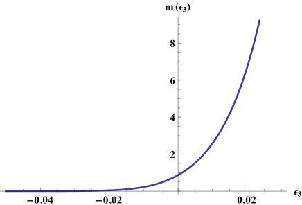
Figure 3: The figure shows the dependence of $m=\left(\frac{M_{5}}{M_{6}}\right)^{2}$ on $\epsilon_{3}$. The statement that MSSM requires small threshold corrections at the GUT scale translates to anisotropic compactification.

The coefficients ${\cal G,H,I}$ and ${\cal N}$ are given in Table 5 in Appendix C. To analyze the GUT scale threshold corrections, we fix $\alpha_{GUT}^{-1}$ to be 24 in all further calculations. Benchmark points are shown in Table 4. The ratio of $M_{5}$ and $M_{6}$ = $m$, depends only on $\epsilon_{3}$ and is shown in Fig 3. The value of m sets the hierarchy between the two compactification scales, $M_{5}$ and $M_{6}$. We analyzed the particle spectrum at intermediate energies in the cases when (i) $M_{5}\ \ll\ M_{6}$ (ii) $M_{6}\ \ll\ M_{5}$ and (iii) $M_{5}\ =\ M_{6}$ to determine the scale associated with the unication of SU(3) $\times$ SU(2) $\times$ U(1)_Y gauge groups. Also, to determine if the SU(6) was broken down to a subgroup at these intermediate scales, reflecting the two step GUT breaking procedure that we employed. We find two unification scales - the SM gauge group unify to an SU(3) $\times$ SU(3) $\times$ U(1) at the scale $M_{5}$ in all the above three cases. Then further at the scale $\sqrt{M_{5}^{2}+M_{6}^{2}}$ there is another unification scale associated with SU(3) $\times$ SU(3) unification to the SU(6) GUT. On the other hand, we do not find a scale associated with the breaking to SU(5) $\times$ U(1)_X which is a typical feature of local GUT breaking as noted in [31].

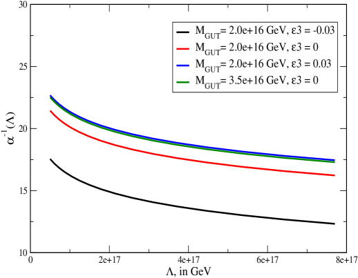
Figure 4: Once $M_{5}$ and $M_{6}$ are solved for uniquely, we are left with a curve in the $\alpha^{-1}-\Lambda$ plane, as expressed in Eq. (84). The unified coupling at the cut-off scale is in the perturbative regime.

It is also interesting to note that the standard scenarios of the MSSM can be embedded in an isotropic or anisotropic orbifold. We find that in the anisotropic as well as isotropic ($M_{5}\sim M_{6}$) cases, the lowest compactification scale is around the 4D GUT scale, making it possible to connect the compactification scale and the 4D GUT scale. For three benchmark points, the curve in the $\alpha^{-1}(\Lambda)-\Lambda$ plane, from Eq. (84) is shown in Fig 4. Finally we note that the values of $\alpha^{-1}(\Lambda),\Lambda$ are not consistent with perturbative heterotic string boundary conditions. In particular, since $\alpha$ depends only of the logarithm of $\Lambda$, it is not possible to embed this orbifold GUT into the weakly coupled regime of the heterotic string, where value of the GUT coupling constant at the string scale is given by[42]:

$$\alpha^{-1}(\Lambda=M_{string})=\frac{1}{8}\left(\frac{M_{PL}}{M_{string}}\right)^{2}$$ (85)

	$\epsilon_{3}$	$M_{5}$	$M_{6}$	$\Lambda$	$\alpha^{-1}(\Lambda)$
Point 1	-3.0%	$0.174\times 10^{16}$	$2.08\times 10^{16}$	$6.0\times 10^{17}$	13.57
Point 2	0.0 %	$3.39\times 10^{16}$	$3.64\times 10^{16}$	$6.0\times 10^{17}$	17.47
Point 3	+3.0 %	$1.37\times 10^{17}$	$3.44\times 10^{16}$	$6.0\times 10^{17}$	18.70

Table 4: The table shows a benchmark point for choice 1 and choice 2. We fix $\alpha_{GUT}^{-1}$ to be 24 and $M_{GUT}$ to be $3\times 10^{16}$ GeV for both the points. The smallest compactification scale is naturally of the order of the 4D GUT scale. All scales are in GeV.

5 Summary

In this work, we discussed a supersymmetric SU(6) gauge theory on an orbifold with the topology of a real projective plane. The compact space was obtained in two steps by orbifolding a rotation and a freely-acting roto-translation. In the process, the gauge symmetry was broken down from SU(6) to SU(5) $\times$ U(1)_X and the N=4 SUSY was reduced to N=2. To further break the SU(5) down to the Standard Model, we introduced a non-zero Wilson line along the fifth and sixth directions. This helped to eliminate the unwanted light states like the Higgs triplets and to break N=2 to N=1 SUSY.

We calculated the Kaluza Klein spectrum of states coming from this orbifolding and also calculated the threshold corrections coming from these states at the 4D grand unification scale. We find that the threshold corrections coming from the KK states due to compactification on an orbifold with the topology of $RP^{2}$ are at the percent level allowing for realistic 4D MSSM. The solutions allow for threshold corrections to be between $\{-3\%,+2\%\}$ allowing for the standard universal gaugino mass scenario like CMSSM or the non-universal gaugino mass scenarios (especially lighter gluinos as discussed in [43, 22]). There have been previous calculations of threshold corrections in orbifold GUT models on various orbifolds with local and non-local GUT breaking. We have already pointed out that unlike in other scenarios we do not get power law running of couplings above the compactification scale due to the large N=2 in 6D. The advantage of not having such large power-law corrections is that we do not lose any predictability due to UV scale physics. We should point out that in the work of Trapletti [31], the author considered a non-local GUT breaking and concluded that the running of couplings stops precisely above the compactification scale. We however find that there are small finite threshold corrections at all scales.

Our analysis was a bottom-up approach studying the phenomenology of models on an orbifold with the topology of a projective plane. It would be interesting to explore the possibility of embedding these orbifold GUTs into a more fundamental theory, like string theory. On the other hand, it would be equally interesting to study low energy features like SUSY breaking and spectra. Finally, since the compactification scale is naturally around the 4D GUT scale or larger, one does not have to worry about proton decay from dimension 6 operators. Moreover, proton decay from dimension 5 operators vanishes due to a discrete R symmetry.

6 Acknowledgments

We would like to thank Michael Ratz for useful discussions. The authors acknowledge partial support from DOE grant DOE/ER/01545-893. AA would also like to thank Konstantin Bobkov and Ben Dundee for their helpful insights.

Appendix A Kaluza-Klein Integrals

In order to compute the threshold corrections coming from an infinite tower of Kaluza-Klein states, we would like to evaluate the following integral (See Eq.(74)):

$$\sum_{(m,n)\in Z}\int_{\xi}^{\infty}\frac{dt}{t}e^{-\pi t\frac{M_{(m,n)}^{2}}{\mu^{2}}}e^{-\pi\chi t}$$ (86)

where, $\chi$ and $\xi$ are IR and UV regulators, and the $M_{(m,n)}$ are the masses of the $(m,n)^{\text{th}}$ KK mode. In the presence of Wilson lines they are given by:

$$M_{(m,n)}^{2}=\frac{(m+\rho_{1})^{2}}{R_{5}^{2}}+\frac{(n+\rho_{2})^{2}}{R_{6}^{2}}$$ (87)

where in the scenario that we have, $\rho_{1}$ can be either 0 or 2 and $\rho_{2}$ is always 0. In general, we can solve the integral following Ghilencea [41] who evaluates the integral for the cases of one and two extra-dimensions. Again, in the current scenario that we have, we find that we only need to evaluate this integral in its one-dimensional limit. We follow Ghilencea and evaluate a 1-dimensional Kaluza-Klein integral of the form:

$${\cal R}_{1}\left[\xi,\rho,\delta\right]=\sum_{m\in Z}^{{}^{\prime}}\int_{\xi}^{\infty}\frac{dt}{t}e^{-\pi t\left[(m+\rho)^{2}+\delta\right]}$$ (88)

where the prime over the summation in the second term represents that m $\neq$ 0, but runs over all other integer values.

We can make use of the Poisson re-summation formula:

$$\sum_{n\in Z}e^{-\pi A(n+\sigma)^{2}}=\frac{1}{\sqrt{A}}\sum_{\tilde{n}\in Z}e^{-\pi A^{-1}\tilde{n}^{2}+2i\pi\tilde{n}\sigma}$$ (89)

to evaluate this integral. We have,

$${\cal R}_{1}\left[\xi,\rho,\delta\right] = \int_{\xi}^{\infty}\frac{dt}{t}\left[-e^{-\pi t\rho^{2}}+\sum_{m}e^{-\pi t(m+\rho)^{2}}\right]e^{-\pi\delta t}$$ (90)

$$= \int_{\xi}^{\infty}\frac{dt}{t}\left[-e^{-\pi t\rho^{2}}+\frac{1}{\sqrt{t}}+\frac{1}{\sqrt{t}}\sum_{m}^{{}^{\prime}}e^{-\pi m^{2}/t+2i\pi m\rho}\right]e^{-\pi\delta t}$$

$$= -\Gamma\left[0,\pi\xi(\delta+\rho^{2})\right]+\frac{2e^{-\pi\delta\xi}}{\sqrt{\xi}}+2\pi\sqrt{\delta}\text{Erf}\left[\sqrt{\pi\delta\xi}\right]$$

$$- \text{log}|2\ \text{sin}\pi(\rho+i\sqrt{\delta})|^{2}$$

where, it has been assumed that $\xi\ll 1$ while evaluating the integral $\int_{\xi}^{\infty}\frac{dt}{t}e^{-\pi m^{2}/t-\pi\delta t}$ and Ghilencea[41] shows that the error by doing so vanishes when $\xi$ is small.

We summarize the result of this integral in various useful limits:

• (m,n) = (0,0)

  $$\int_{\xi}^{\infty}\frac{dt}{t}e^{-\pi t\frac{\rho_{1}^{2}}{R_{5}^{2}\mu^{2}}}e^{-\pi\chi t} = \int_{\xi}^{\infty}\frac{dt}{t}e^{-\pi(\rho+\chi)t}$$ (91)

  $$= \Gamma\left[0,\pi\xi(\chi+\rho)\right]$$

  where $\rho=\frac{\rho_{1}^{2}}{R_{5}^{2}\mu^{2}}+\frac{\rho_{2}^{2}}{R_{6}^{2}\mu^{2}}$

• n=0, m $\neq$ 0

  $$\sum_{m\in Z}^{{}^{\prime}}\int_{\xi}^{\infty}\frac{dt}{t}e^{-\pi t\frac{\frac{(m+\rho_{1})^{2}}{R_{5}^{2}}+\frac{\rho_{2}^{2}}{R_{6}^{2}}}{\mu^{2}}}e^{-\pi\chi t} = \sum_{m\in Z}^{{}^{\prime}}\int_{\xi\nu_{1}}^{\infty}\frac{dt}{t}e^{-\pi t(m+\rho_{1})^{2}}e^{-\pi\frac{\delta_{1}}{\nu_{1}}t}$$ (92)

  $$= {\cal R}_{1}\left[\xi\nu_{1},\rho_{1},\frac{\delta_{1}}{\nu_{1}}\right]$$

  where, $\nu_{1}=\frac{1}{\mu^{2}R_{5}^{2}}$ and $\delta_{1}=\chi+\frac{\rho_{2}^{2}}{\mu^{2}R_{6}^{2}}$.

• m=0, n $\neq$ 0
  Similar to the previous case with some parameters interchanged, we have:

  $$\sum_{n\in Z}^{{}^{\prime}}\int_{\xi}^{\infty}\frac{dt}{t}e^{-\pi t\frac{\frac{\rho_{1}^{2}}{R_{5}^{2}}+\frac{(n+\rho_{2})^{2}}{R_{6}^{2}}}{\mu^{2}}}e^{-\pi\chi t} = \sum_{n\in Z}^{{}^{\prime}}\int_{\xi\nu_{2}}^{\infty}\frac{dt}{t}e^{-\pi t(n+\rho_{2})^{2}}e^{-\pi\frac{\delta_{2}}{\nu_{2}}t}$$ (93)

  $$= {\cal R}_{1}\left[\xi\nu_{2},\rho_{2},\frac{\delta_{2}}{\nu_{2}}\right]$$

  where, $\nu_{2}=\frac{1}{\mu^{2}R_{6}^{2}}$ and $\delta_{2}=\chi+\frac{\rho_{1}^{2}}{\mu^{2}R_{5}^{2}}$

• Since the spectrum we are interested in has states that live either at odd or even integers, it is write down the result of this integral in these limit that the summation is over either even or odd integers:
  n=0, m $\neq$ 0; m=even
  

  $${\cal R}_{1}^{E}\left[\xi\nu_{1},\rho_{1},\frac{\delta_{1}}{\nu_{1}}\right] = \sum_{m\in Z}^{{}^{\prime}}\int_{\xi}^{\infty}\frac{dt}{t}e^{-\pi t\frac{\frac{(2m+\rho_{1})^{2}}{R_{5}^{2}}+\frac{\rho_{2}^{2}}{R_{6}^{2}}}{\mu^{2}}}e^{-\pi\chi t}$$ (94)

  $$= \sum_{m\in Z}^{{}^{\prime}}\int_{\xi}^{\infty}\frac{dt}{t}e^{-4\pi t\frac{\frac{(m+\frac{\rho_{1}}{2})^{2}}{R_{5}^{2}}+\frac{\rho_{2}^{2}}{4R_{6}^{2}}}{\mu^{2}}}e^{-\pi\chi t/4}$$

  $$= \sum_{m\in Z}^{{}^{\prime}}\int_{4\xi\nu_{1}}^{\infty}\frac{dt}{t}e^{-\pi t(m+\rho_{1})^{2}}e^{-\pi\frac{\delta_{1}}{4\nu_{1}}t}$$

  $$= {\cal R}_{1}\left[4\xi\nu_{1},\frac{\rho_{1}}{2},\frac{\delta_{1}}{4\nu_{1}}\right]$$

  where, $\nu_{1}=\frac{1}{\mu^{2}R_{5}^{2}}$ and $\delta_{1}=\chi+\frac{\rho_{2}^{2}}{\mu^{2}R_{6}^{2}}$ is the same as previously defined.
  n=0, m $\neq$ 0; m=odd
  

  $${\cal R}_{1}^{O}\left[\xi\nu_{1},\rho_{1},\frac{\delta_{1}}{\nu_{1}}\right] = \sum_{m\in Z}\int_{\xi}^{\infty}\frac{dt}{t}e^{-\pi t\frac{\frac{(2m-1+\rho_{1})^{2}}{R_{5}^{2}}+\frac{\rho_{2}^{2}}{R_{6}^{2}}}{\mu^{2}}}e^{-\pi\chi t}$$

  $$= \sum_{m\in Z}\int_{\xi}^{\infty}\frac{dt}{t}e^{-4\pi t\frac{\frac{(m+\frac{\rho_{1}-1}{2})^{2}}{R_{5}^{2}}+\frac{\rho_{2}^{2}}{4R_{6}^{2}}}{\mu^{2}}}e^{-\pi\chi t/4}$$

  $$= \int_{\xi\nu_{1}}^{\infty}\frac{dt}{t}e^{-\pi t\frac{(\rho_{1}-1)^{2}}{4}}e^{-\pi\frac{\delta_{1}}{4\nu_{1}}t}$$

  $$\quad+\sum_{m\in Z}^{{}^{\prime}}\int_{4\xi\nu_{1}}^{\infty}\frac{dt}{t}e^{-\pi t(m+\frac{\rho_{1}-1}{2})^{2}}e^{-\pi\frac{\delta_{1}}{4\nu_{1}}t}$$

  $$= \Gamma\left[0,\pi\xi(\nu_{1}(\rho_{1}-1)^{2}+\delta_{1})\right]+{\cal R}_{1}\left[4\xi\nu_{1},\frac{\rho_{1}-1}{2},\frac{\delta_{1}}{4\nu_{1}}\right]$$

  In order to write the result of the integral in terms of the original ${\cal R}_{1}$, we separate the zeroth term from the rest in the summation. It is also useful to note that the function ${\cal R}_{1}$ is even in $\rho$ and hence:

  $${\cal R}_{1}\left[\xi,\rho,\delta\right]={\cal R}_{1}\left[\xi,-\rho,\delta\right]$$ (96)

Appendix B Useful Limits of Relevant Functions

The result of the Kaluza-Klein integrals were evaluated in the previous section, in terms of the two functions, $\Gamma[0,\pi\xi\chi]$ and ${\cal R}_{1}\left[\xi,\rho,\delta\right]$. $\chi$ and $\xi$ are the regulators and in the limit that they are zero, we can replace them with the relevant mass scales.

$$Q^{2}\equiv\pi e^{\gamma}\chi\mu^{2}\Big{|}_{\chi\rightarrow 0}\qquad\Lambda^{2}\equiv\frac{\mu^{2}}{\xi}\Big{|}_{\xi\rightarrow 0}$$ (97)

As evaluated in the previous section:

$${\cal R}_{1}\left[\xi,\rho,\delta\right] = -\Gamma\left[0,\pi\xi(\delta+\rho^{2})\right]+\frac{2e^{-\pi\delta\xi}}{\sqrt{\xi}}+2\pi\sqrt{\delta}\text{Erf}\left[\sqrt{\pi\delta\xi}\right]$$

$$\qquad-\text{log}|2\ \text{sin}\pi(\rho+i\sqrt{\delta})|^{2}$$

We use the following expansions:

$$-\Gamma\left[0,z\right] = \gamma+\text{ln}\ z+\sum_{k\geq 1}\frac{(-z)^{k}}{k!\ k}\qquad z>0$$ (98)

$$\text{Erf}\left[x\right] = \frac{2x}{\sqrt{\pi}}-\frac{2x^{3}}{3\sqrt{\pi}}+{\cal O}(x^{5})\qquad x\ll 1$$ (99)

Then,

$$\Gamma\left[0,\pi\xi\chi\right] = -\gamma-\text{ln}\ \pi\xi\chi$$ (100)

$$= -\text{ln}\ \pi\frac{e^{\gamma}\mu^{2}Q^{2}}{\Lambda^{2}\pi e^{\gamma}\mu^{2}}$$

$$= -\text{ln}\ \frac{Q^{2}}{\Lambda^{2}}$$

With these approximations, ${\cal R}_{1}\left[\xi,\rho,\delta\right]$ simplifies to:

$${\cal R}_{1}\left[\xi,\rho,\delta\right] = -\text{ln}\left[4\pi e^{-\gamma}\frac{1}{\xi}e^{-2/\sqrt{\xi}}\right]-\text{ln}\left|\frac{\text{sin}(\rho+i\sqrt{\delta})}{\pi(\rho+i\sqrt{\delta})}\right|^{2}$$ (101)

We summarize, the various terms that come up in the calculation of threshold corrections in Section 3. In the expressions below, we have also introduced the compactifications scales $M_{5}=\sqrt{\pi e^{\gamma}}/R_{5}$ and $M_{6}=\sqrt{\pi e^{\gamma}}/R_{6}$.

$$\Gamma\left[0,\pi\xi\chi\right] = \text{ln}\frac{\Lambda^{2}}{Q^{2}}$$

$$\Gamma\left[0,\pi\xi\nu_{1}\right] = -\gamma-\text{ln}\frac{\pi}{\Lambda^{2}R_{5}^{2}}$$

$$= -\text{ln}\left[\frac{M_{5}^{2}}{\Lambda^{2}}\right]$$

$$\Gamma\left[0,\pi\xi\nu_{2}\right] = -\gamma-\text{ln}\frac{\pi}{\Lambda^{2}R_{6}^{2}}$$

$$= -\text{ln}\left[\frac{M_{6}^{2}}{\Lambda^{2}}\right]$$

$${\cal R}_{1}\left[4\xi\nu_{1},0,\frac{\chi}{4\nu_{1}}\right] = -\text{ln}\left[\pi e^{-\gamma-\Lambda R_{5}}(\Lambda R_{5})^{2}\right]$$

$${\cal R}_{1}\left[4\xi\nu_{1},\frac{1}{2},\frac{\chi}{4\nu_{1}}\right] = -\text{ln}\left[\pi e^{-\gamma-\Lambda R_{5}}(\Lambda R_{5})^{2}\right]-\text{ln}\left[\frac{2}{\pi}\right]^{2}$$

$${\cal R}_{1}\left[4\xi\nu_{2},0,\frac{\chi}{4\nu_{2}}\right] = -\text{ln}\left[\pi e^{-\gamma-\Lambda R_{6}}(\Lambda R_{6})^{2}\right]$$

$${\cal R}_{1}\left[4\xi\nu_{2},\frac{1}{2},\frac{\chi}{4\nu_{2}}\right] = -\text{ln}\left[\pi e^{-\gamma-\Lambda R_{6}}(\Lambda R_{6})^{2}\right]-\text{ln}\left[\frac{2}{\pi}\right]^{2}$$

$$\Gamma\left[0,\pi\xi\left(\frac{\nu_{1}}{4}+\frac{\nu_{2}}{4}\right)\right] = -\text{ln}\left[\frac{M_{5}^{2}+M_{6}^{2}}{4\Lambda^{2}}\right]$$

Appendix C 6D $\rightarrow$ 4D matching

We calculated the corrections to the gauge couplings coming from the KK states of the 6D orbifold model that was constructed. At the lowest compactification scale (largest compactification radius), we said that the couplings from 4D MSSM and 6D orbifold model should match. In this section, we will compare the two sets of equations, from the two theories:

$$\alpha_{i}^{-1}(Q) = \alpha^{-1}(\Lambda)+\sum_{\rho}\Omega_{i,\rho}(Q)$$

$$\alpha_{i}^{-1}(Q) = \alpha_{GUT}^{-1}+\frac{b_{i}}{2\pi}log\frac{M_{GUT}}{Q}-\alpha_{GUT}^{-1}\frac{\epsilon_{3}}{(1+\epsilon_{3})}\delta_{i3}$$

and solve for the three scales of the orbifold model, $\Lambda$, $M_{5}$, and $M_{6}$ as well as coupling constant, $\alpha$ at the cut-off scale.

Since the two expressions have to match at all scales below the smallest compactification scale of the orbifold model, we can rewrite the above two equations as:

$$\alpha_{GUT}^{-1} + \frac{b_{i}}{4\pi}\text{ln}\frac{M_{GUT}^{2}}{Q^{2}}-\alpha_{GUT}^{-1}\frac{\epsilon_{3}}{(1+\epsilon_{3})}\delta_{i3}$$

$$= \alpha^{-1}(\Lambda)+\frac{b_{i}^{++}(I_{\rho}=0)}{4\pi}\text{ln}\frac{\Lambda^{2}}{Q^{2}}+\left(\frac{b_{i}^{+-}(I_{\rho}=0)+b_{i}^{-+}(I_{\rho}=0)}{4\pi}\right)\text{ln}\left[\frac{\pi\Lambda}{2M_{5}}\right]^{2}$$

$$+ \left(\frac{b_{i}^{+-}(I_{\rho}=0)+b_{i}^{--}(I_{\rho}=0)}{4\pi}\right)\text{ln}\left[\frac{\pi\Lambda}{2M_{6}}\right]^{2}+\frac{b_{i}^{+-}(I_{\rho}=2)}{4\pi}\text{ln}\left[\frac{4\Lambda^{2}}{M_{5}^{2}+M_{6}^{2}}\right]$$

where we have used the complete expression we estimated for the corrections to couplings in 83.

We use the following redefinitions:

$$\frac{b_{i}^{MSSM}}{4\pi}=\frac{b_{i}^{++}(I_{\rho}=0)}{4\pi} = \beta_{i}$$

$$\frac{b_{i}^{+-}(I_{\rho}=0)+b_{i}^{-+}(I_{\rho}=0)}{4\pi} = -A_{i}$$

$$\frac{b_{i}^{+-}(I_{\rho}=0)+b_{i}^{--}(I_{\rho}=0)}{4\pi} = -B_{i}$$

$$\frac{b_{i}^{+-}(I_{\rho}=2)}{4\pi} = -C_{i}$$ (104)

and

$$(A_{i}+B_{i})\text{ln}\left[\frac{\pi}{2}\right]^{2}+C_{i}\text{ln}\left[4\right]=D_{i}$$ (105)

and hence end up with a set of three equations that can be simply written as:

$$\alpha_{GUT}^{-1} - \alpha^{-1}(\Lambda)-\alpha_{GUT}^{-1}\frac{\epsilon_{3}}{(1+\epsilon_{3})}\delta_{i3}-\beta_{i}\text{ln}\frac{\Lambda^{2}}{M_{GUT}^{2}}$$ (106)

$$+ A_{i}\text{ln}\frac{\Lambda^{2}}{M_{5}^{2}}+B_{i}\text{ln}\frac{\Lambda^{2}}{M_{6}^{2}}+C_{i}\text{ln}\frac{\Lambda^{2}}{M_{5}^{2}+M_{6}^{2}}+D_{i}=0$$

where, $A_{i}=A_{1i}+A_{2i}$ and $i=1,2,3$. We look at the equations corresponding (i) (i = 1) - (i =2) (ii) i = 2 (iii) i = 3 and solve for $\Lambda$, $M_{5}$, and $M_{6}$. It is usually considered that the 4D unification scale is around $3.0\times 10^{16}$ GeV and the couplings at this scale are unified at $\alpha_{GUT}^{-1}=24$. In standard scenarios of MSSM with gaugino mass unification, $\epsilon_{3}=-3\%$. Depending of the spectrum of low energy SUSY, these quantities are subject to change. The first equation we get by simplifying Eq. (106) for (i = 1) - (i =2) is:

$$-(\beta_{1}-\beta_{2})\text{ln}\frac{\Lambda^{2}}{M_{GUT}^{2}} + (A_{1}-A_{2})\text{ln}\frac{\Lambda^{2}}{M_{5}^{2}}+(B_{1}-B_{2})\text{ln}\frac{\Lambda^{2}}{M_{6}^{2}}$$ (107)

$$+ (C_{1}-C_{2})\text{ln}\frac{\Lambda^{2}}{M_{5}^{2}+M_{6}^{2}}+(D_{1}-D_{2})=0$$

Defining, $\frac{\Lambda^{2}}{M_{5}^{2}}=X$ and $\frac{\Lambda^{2}}{M_{6}^{2}}=Y$, we get:

$$\text{ln}\frac{\Lambda^{2}}{M_{GUT}^{2}} = \left(\frac{A_{1}-A_{2}}{\beta_{1}-\beta_{2}}\right)\text{ln}X+\left(\frac{B_{1}-B_{2}}{\beta_{1}-\beta_{2}}\right)\text{ln}Y$$ (108)

$$- \left(\frac{C_{1}-C_{2}}{\beta_{1}-\beta_{2}}\right)\text{ln}\left(\frac{1}{X}+\frac{1}{Y}\right)+\left(\frac{D_{1}-D_{2}}{\beta_{1}-\beta_{2}}\right)$$

Next, we look at Eq (106) when $i=2$:

$$\alpha_{GUT}^{-1} - \alpha^{-1}(\Lambda)-\beta_{2}\text{ln}\frac{\Lambda^{2}}{M_{GUT}^{2}}$$ (109)

$$+ A_{2}\text{ln}X+B_{2}\text{ln}Y-C_{2}\text{ln}\left(\frac{1}{X}+\frac{1}{Y}\right)+D_{2}=0$$

Then, using the expression we just derived in Eq. (108), we get an expression for $\alpha^{-1}(\Lambda)$:

$$\alpha^{-1}(\Lambda) = \alpha_{GUT}^{-1}+\left[A_{2}-\beta_{2}\left(\frac{A_{1}-A_{2}}{\beta_{1}-\beta_{2}}\right)\right]\text{ln}X+\left[B_{2}-\beta_{2}\left(\frac{B_{1}-B_{2}}{\beta_{1}-\beta_{2}}\right)\right]\text{ln}Y$$

$$- \left[C_{2}-\beta_{2}\left(\frac{C_{1}-C_{2}}{\beta_{1}-\beta_{2}}\right)\right]\text{ln}\left(\frac{1}{X}+\frac{1}{Y}\right)+\left[D_{2}-\beta_{2}\left(\frac{D_{1}-D_{2}}{\beta_{1}-\beta_{2}}\right)\right]$$

Finally, we look at Eq (106) when $i=3$, and simplify it using the relations obtained in Eqs. (108 & LABEL:invastr) and we get a final expression:

$$\left[A_{3}-A_{2}+\left(\frac{A_{1}-A_{2}}{\beta_{1}-\beta_{2}}\right)(\beta_{2}-\beta_{3})\right]\text{ln}X + \left[B_{3}-B_{2}+\left(\frac{B_{1}-B_{2}}{\beta_{1}-\beta_{2}}\right)(\beta_{2}-\beta_{3})\right]\text{ln}Y$$

$$-\left[C_{3}-C_{2}+\left(\frac{C_{1}-C_{2}}{\beta_{1}-\beta_{2}}\right)(\beta_{2}-\beta_{3})\right]\text{ln}\left(\frac{1}{X}+\frac{1}{Y}\right) + \left[D_{3}-D_{2}+\left(\frac{D_{1}-D_{2}}{\beta_{1}-\beta_{2}}\right)(\beta_{2}-\beta_{3})\right]$$

$$-\alpha^{-1}_{GUT}\frac{\epsilon_{3}}{1+\epsilon_{3}} = 0$$ (111)

The above three equations can be rewritten in a simple manner as (in the order Eq. (111), (108), (LABEL:invastr)):

$${\cal A}\text{ln}X+{\cal B}\text{ln}Y-{\cal C}\text{ln}\left(\frac{1}{X}+\frac{1}{Y}\right)+{\cal D} = 0$$

$${\cal F}\text{ln}X+{\cal G}\text{ln}Y-{\cal H}\text{ln}\left(\frac{1}{X}+\frac{1}{Y}\right)+{\cal I} = \text{ln}\frac{\Lambda^{2}}{M_{GUT}^{2}}$$

$${\cal K}\text{ln}X+{\cal L}\text{ln}Y-{\cal M}\text{ln}\left(\frac{1}{X}+\frac{1}{Y}\right)+{\cal N} = \alpha^{-1}(\Lambda)$$

with,

$${\cal A} = A_{3}-A_{2}+(A_{1}-A_{2})\left(\frac{\beta_{2}-\beta_{3}}{\beta_{1}-\beta_{2}}\right),$$

$${\cal B} = B_{3}-B_{2}+(B_{1}-B_{2})\left(\frac{\beta_{2}-\beta_{3}}{\beta_{1}-\beta_{2}}\right),$$

$${\cal C} = C_{3}-C_{2}+(C_{1}-C_{2})\left(\frac{\beta_{2}-\beta_{3}}{\beta_{1}-\beta_{2}}\right),$$

$${\cal D} = D_{3}-D_{2}+(D_{1}-D_{2})\left(\frac{\beta_{2}-\beta_{3}}{\beta_{1}-\beta_{2}}\right)-\alpha_{GUT}^{-1}\frac{\epsilon_{3}}{(1+\epsilon_{3})}$$

$${\cal F} = \frac{A_{1}-A_{2}}{\beta_{1}-\beta_{2}},$$

$${\cal G} = \frac{B_{1}-B_{2}}{\beta_{1}-\beta_{2}},$$

$${\cal H} = \frac{C_{1}-C_{2}}{\beta_{1}-\beta_{2}},$$

$${\cal I} = \frac{D_{1}-D_{2}}{\beta_{1}-\beta_{2}},$$

$${\cal K} = A_{2}-\beta_{2}\left(\frac{A_{1}-A_{2}}{\beta_{1}-\beta_{2}}\right),$$

$${\cal L} = B_{2}-\beta_{2}\left(\frac{B_{1}-B_{2}}{\beta_{1}-\beta_{2}}\right),$$

$${\cal M} = C_{2}-\beta_{2}\left(\frac{C_{1}-C_{2}}{\beta_{1}-\beta_{2}}\right),$$

$${\cal N} = D_{2}-\beta_{2}\left(\frac{D_{1}-D_{2}}{\beta_{1}-\beta_{2}}\right)+\alpha^{-1}_{GUT},$$

These quantities can be calculated using the beta-function coefficients given in Table. 3. The numerical values of all the above coefficients are summarized in Table 5.

Coefficient	Value
${\cal A}$	$-\frac{3}{7\pi}$
${\cal B}$	$\frac{6}{7\pi}$
${\cal C}$	$-\frac{3}{7\pi}$
${\cal D}(\epsilon_{3})$	$-\alpha_{GUT}^{-1}\frac{\epsilon_{3}}{1+\epsilon_{3}}-\frac{6}{7\pi}\text{ln}\frac{4}{\pi}$
${\cal F}$	$\frac{4}{7}$
${\cal G}$	$\frac{6}{7}$
${\cal H}$	$-\frac{3}{7}$
${\cal I}$	$-\frac{3}{7}\text{ln}4-\frac{20}{7}\text{ln}\frac{2}{\pi}$
${\cal K}$	$-\frac{9}{14\pi}$
${\cal L}$	$-\frac{12}{7\pi}$
${\cal M}$	$-\frac{9}{14\pi}$
${\cal N}$	$\alpha^{-1}_{GUT}-\frac{6}{7\pi}\text{ln}2-\frac{33}{7\pi}\text{ln}\frac{2}{\pi}$

Table 5: The coefficients in the expression Eq. (LABEL:threeeq)

With these coefficients, we get a simple quadratic equation in terms in of the variables X and Y:

$$\left(\frac{Y}{X}\right)^{2}+\frac{Y}{X}-\text{Exp}\ \left(-\frac{7\pi{\cal D}(\epsilon_{3})}{3}\right)=0$$ (113)

Recall that $X=\frac{\Lambda^{2}}{M_{5}^{2}}$ and $Y=\frac{\Lambda^{2}}{M_{6}^{2}}$, which implies that the above equation turns into a quadratic equation in $\left(\frac{M_{5}}{M_{6}}\right)^{2}$ with the solution.

$$M_{5}^{2} = \frac{-1\pm\sqrt{1+4\text{Exp}\ \left(-\frac{7\pi{\cal D}(\epsilon_{3})}{3}\right)}}{2}M_{6}^{2}$$ (114)

which we write as $M_{5}=\sqrt{m(\epsilon_{3})}M_{6}$. The slope $m$, is the positive solution from the above expression and is shown in Fig. 3. The other two equations then yield us $M_{5}$ and $M_{6}$ uniquely and one expression relating $\alpha^{-1}(\Lambda)$ and $\Lambda$.

$$M_{5} = \left(m(\epsilon_{3})^{({\cal G-H})/2}(m(\epsilon_{3})+1)^{{\cal H}/2}e^{{\cal I}/2}\right)M_{GUT}$$

$$M_{6} = \left(m(\epsilon_{3})^{({\cal G-H}-1)/2}(m(\epsilon_{3})+1)^{{\cal H}/2}e^{{\cal I}/2}\right)M_{GUT}$$

$$\alpha^{-1}(\Lambda) = -\frac{3}{\pi}\text{ln}\frac{\Lambda^{2}}{M_{GUT}^{2}}+\frac{3}{\pi}\text{ln}\left(m(\epsilon_{3})^{({\cal G-H})}(m(\epsilon_{3})+1)^{{\cal H}}e^{{\cal I}}\right)$$ (115)

$$+ \text{ln}\left(m(\epsilon_{3})^{({\cal L-M})}(m(\epsilon_{3})+1)^{{\cal M}}e^{{\cal N}}\right)$$

These expressions are plotted in figure.

References

• [1] S. Dimopoulos, S. Raby, and F. Wilczek, Phys. Rev. D24 (1981) 1681–1683.
• [2] S. Dimopoulos and H. Georgi, Nucl. Phys. B193 (1981) 150.
• [3] L. E. Ibanez and G. G. Ross, Phys. Lett. B105 (1981) 439.
• [4] N. Sakai, Zeit. Phys. C11 (1981) 153. Uekusa:2008iz
• [5] M. B. Einhorn and D. R. T. Jones, Nucl. Phys. B196 (1982) 475.
• [6] W. J. Marciano and G. Senjanović, Phys. Rev. D25 (1982) 3092.
• [7] R. Dermisek, A. Mafi and S. Raby, Phys. Rev. D 63, 035001 (2001) [hep-ph/0007213].
• [8] H. Murayama and A. Pierce, Phys. Rev. D65 (2002) 055009, [hep-ph/0108104].
• [9] Makoto Miura [Super-Kamiokande Collaboration], ICHEP 2010.
• [10] K. R. Dienes, E. Dudas and T. Gherghetta, Phys. Lett. B 436, 55 (1998) [hep-ph/9803466].
• [11] K. R. Dienes, E. Dudas and T. Gherghetta, Nucl. Phys. B 537, 47 (1999) [hep-ph/9806292].
• [12] Y. Kawamura, Prog. Theor. Phys.  105, 999 (2001) [hep-ph/0012125].
• [13] L. J. Hall and Y. Nomura, Phys. Rev. D 64, 055003 (2001) [hep-ph/0103125].
• [14] T. Asaka, W. Buchmuller and L. Covi, Phys. Lett. B 523, 199 (2001) [hep-ph/0108021].
• [15] R. Contino, L. Pilo, R. Rattazzi and E. Trincherini, Nucl. Phys. B 622, 227 (2002) [hep-ph/0108102].
• [16] A. Hebecker and J. March-Russell, Nucl. Phys. B 613, 3 (2001) [hep-ph/0106166].
• [17] L. J. Hall, Y. Nomura and D. Tucker-Smith, Nucl. Phys. B 639, 307 (2002) [hep-ph/0107331].
• [18] R. Dermisek and A. Mafi, problem,” Phys. Rev. D 65, 055002 (2002) [hep-ph/0108139].
• [19] L. J. Hall and Y. Nomura, Phys. Rev. D 65, 125012 (2002) [hep-ph/0111068].
• [20] H. D. Kim and S. Raby, JHEP 0301, 056 (2003) [hep-ph/0212348].
• [21] B. Dundee, S. Raby and A. Wingerter, Compactifications,” Phys. Rev. D 78, 066006 (2008) [arXiv:0805.4186 [hep-th]].
• [22] A. Anandakrishnan and S. Raby, SUSY Breaking,” Phys. Rev. D 83, 075008 (2011) [arXiv:1101.1976 [hep-ph]].
• [23] L. J. Dixon, J. A. Harvey, C. Vafa and E. Witten, Nucl. Phys. B 261, 678 (1985).
• [24] L. J. Dixon, J. A. Harvey, C. Vafa and E. Witten, Nucl. Phys. B 274, 285 (1986).
• [25] J. D. Breit, B. A. Ovrut and G. C. Segre, Phys. Lett. B 158, 33 (1985).
• [26] L. E. Ibanez, J. E. Kim, H. P. Nilles and F. Quevedo, U(1)**n,” Phys. Lett. B 191, 282 (1987).
• [27] V. S. Kaplunovsky, Nucl. Phys. B 307, 145 (1988) [Erratum-ibid. B 382, 436 (1992)] [hep-th/9205068].
• [28] V. S. Kaplunovsky and J. Louis, string theory,” Phys. Lett. B 306, 269 (1993) [hep-th/9303040].
• [29] L. J. Dixon, V. Kaplunovsky and J. Louis, Nucl. Phys. B 355, 649 (1991).
• [30] A. Hebecker and M. Trapletti, Nucl. Phys. B 713, 173 (2005) [hep-th/0411131].
• [31] M. Trapletti, Mod. Phys. Lett. A 21, 2251 (2006) [hep-th/0611030].
• [32] G. G. Ross, hep-ph/0411057.
• [33] A. Hebecker, JHEP 0401, 047 (2004) [hep-ph/0309313].
• [34] E. A. Mirabelli and M. E. Peskin, Phys. Rev. D 58, 065002 (1998) [hep-th/9712214].
• [35] L. J. Hall, H. Murayama and Y. Nomura, Nucl. Phys. B 645, 85 (2002) [hep-th/0107245].
• [36] R. Dermisek, S. Raby and S. Nandi, Nucl. Phys. B 641, 327 (2002) [hep-th/0205122].
• [37] Y. Hosotani, Phys. Lett. B 126, 309 (1983).
• [38] P. Candelas, G. T. Horowitz, A. Strominger and E. Witten, Nucl. Phys. B 258, 46 (1985).
• [39] E. Witten, Nucl. Phys. B 258, 75 (1985).
• [40] H. M. Lee, S. Raby, M. Ratz, G. G. Ross, R. Schieren, K. Schmidt-Hoberg and P. K. S. Vaudrevange, Phys. Lett. B 694, 491 (2011) [arXiv:1009.0905 [hep-ph]].
• [41] D. M. Ghilencea, Nucl. Phys. B 670, 183 (2003) [hep-th/0305085].
• [42] B. Dundee and S. Raby, arXiv:0808.0992 [hep-th].
• [43] S. Raby, M. Ratz and K. Schmidt-Hoberg, Phys. Lett. B 687, 342 (2010) [arXiv:0911.4249 [hep-ph]].