Nonnegative solutions with a nontrivial nodal set for elliptic equations on smooth symmetric domains

Abstract. We consider a semilinear elliptic equation on a smooth bounded domain $\Omega$ in ${\mathbb{R}}^{2}$, assuming that both the domain and the equation are invariant under reflections about one of the coordinate axes, say the $y$-axis. It is known that nonnegative solutions of the Dirichlet problem for such equations are symmetric about the axis, and, if strictly positive, they are also decreasing in $x$ for $x>0$. Our goal is to exhibit examples of equations which admit nonnegative, nonzero solutions for which the second property fails; necessarily, such solutions have a nontrivial nodal set in $\Omega$. Previously, such examples were known for nonsmooth domains only.

Key words: semilinear elliptic equation, planar domain, nonnegative solutions, nodal set

AMS Classification: 35J61, 35B06, 35B05

1 Introduction and the main result

Consider the elliptic problem

$$\Delta u+f(x^{\prime},u) =0, x\in\Omega,$$ (1.1)

$$u =0, x\in\partial\Omega,$$ (1.2)

where $\Omega$ is a bounded domain in ${\mathbb{R}}^{N}$, $x=(x_{1},x^{\prime})\in{\mathbb{R}}\times{\mathbb{R}}^{N-1}$, and $f:{\mathbb{R}}^{N-1}\times{\mathbb{R}}\to{\mathbb{R}}$ is a continuous function which is locally Lipschitz in the last variable. We assume that $\Omega$ is convex in $x_{1}$ and reflectionally symmetric about the hyperplane

$$H_{0}=\{(x_{1},x^{\prime})\in{\mathbb{R}}\times{\mathbb{R}}^{N-1}:x_{1}=0\}.$$

By a well-known theorem of Gidas, Ni, and Nirenberg [12] and its more general versions for nonsmooth domains, as given by Berestycki and Nirenberg [4] and Dancer [7], each positive solution $u$ of (1.1), (1.2) is even in $x_{1}$:

$$u(-x_{1},x^{\prime})=u(x_{1},x^{\prime})\quad((x_{1},x^{\prime})\in\Omega),$$ (1.3)

and, moreover, $u(x_{1},x^{\prime})$ decreases with increasing $|x_{1}|$:

$$u_{x_{1}}(x_{1},x^{\prime})<0\quad((x_{1},x^{\prime})\in\Omega,x_{1}>0).$$ (1.4)

It is also well-known that this result is not valid in general for nonnegative solutions; consider, for example, the solution $u(x)=1+\cos x$ of the equation $u^{\prime\prime}+u-1=0$ on the interval $\Omega=(-3\pi,3\pi)$. However, as recently proved in [19], nonnegative solutions still enjoy the symmetry property (1.3). Of course, by the Dirichlet boundary condition, (1.4) necessarily fails unless the solution is strictly positive in $\Omega$. A further investigation in [19] revealed that the nodal set of each nonnegative solution $u$ has interesting symmetry properties itself. In particular, each nodal domain of $u$ is convex in $x_{1}$ and symmetric about a hyperplane parallel to $H_{0}$ (a nodal domain refers to a connected component of $\{x\in\Omega:u(x)\neq 0\}$). These results, like those in [4], are valid for fully nonlinear elliptic equations

$$F(x,u,Du,D^{2}u)=0,\quad x\in\Omega,$$ (1.5)

under suitable symmetry assumptions, and their proofs employ the method of moving hyperplanes [2, 21] as the basic geometric technique. Related results can be found in the surveys [3, 15, 16, 17], monographs [9, 11, 20], or more recent papers [5, 8, 6, 10], among others.

In this work, we are concerned with nonnegative solutions which do have a nontrivial nodal set in $\Omega$. In [19], several examples of problems (1.1), (1.2) admitting such solutions were given, including explicit examples with solutions whose nodal set consists of line segments, as well as a more involved construction with non-flat nodal curves. In all these examples, the domain $\Omega$ has corners and it is not even of class $C^{1}$. On the other hand, it was also proved in [19] that for some $C^{1}$ domains $\Omega$ satisfying additional geometric conditions, no solutions with nontrivial nodal sets can exist, no matter how the nonlinearity $f=f(x^{\prime},u)$ is chosen. For example, this is the case if $\Omega$ is a $C^{1}$ planar domain such that the “cups” $\{(x_{1},x_{2})\in\Omega:x_{1}>\lambda\}$, $\lambda\in{\mathbb{R}}$, are all connected and $\partial\Omega$ contains a line segment parallel to the $x_{2}$-axis. These observations raise the following natural question:

Question. Does smoothness of $\Omega$ alone preclude the existence of nonnegative solutions with nontrivial nodal sets for problem (1.1), (1.2)?

The aim of this paper is to show that the answer is negative even when analyticity of both the domain and the nonlinearity is assumed. We stress that the dependence of the nonlinearity on $x^{\prime}$ is essential here. Indeed, a theorem from [18] states that when the class of equations is restricted to the homogeneous ones, $\Delta u+f(u)=0$, and $\Omega$ is smooth, then each nonnegative solution is either identical to 0 (and hence $f(0)=0$) or strictly positive.

Our construction is in two dimensions, hence we use the coordinates $(x,y)$ instead of $(x_{1},x^{\prime})$. We consider affine equations of the form

$$\Delta u+4u+h(y) =0, (x,y)\in\Omega,$$ (1.6)

$$u =0, (x,y)\in\partial\Omega.$$ (1.7)

Here is our main result:

Theorem 1.1.

There exist a continuous function $h:{\mathbb{R}}\to{\mathbb{R}}$ and a bounded analytic domain $\Omega\subset{\mathbb{R}}^{2}$, which is convex in $x$ and symmetric about the vertical axis $H_{0}=\{(0,y):y\in{\mathbb{R}}\}$, such that problem (1.6), (1.7) has a nonnegative solution $u$ whose nodal set in $\Omega$ consists of two analytic curves.

By an analytic domain we mean a Lipschitz domain whose boundary is an analytic submanifold of ${\mathbb{R}}^{2}$. A curve refers to a one-dimensional submanifold of ${\mathbb{R}}^{2}$, possibly with boundary.

The nodal set of the solution $u$, including the boundary of $\Omega$, is plotted in Figure 1. In accordance with [19, Theorem 2.2], each nodal domain of $u$ is symmetric about a line parallel to the $y$-axis, as indicated by dashed lines in Figure 1, and the solution $u$ is symmetric about that line within the nodal domain.

Figure 1: The nodal set (the solid curves) of $u$.

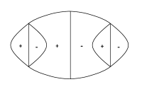
Figure 2: The nodal set and the signs of $v$.

Similarly to [19], our construction links the solutions of (1.6) to some eigenfunction of the Laplacian. Specifically, if $u$ is a solution of (1.6), then $v=u_{x}$ satisfies $\Delta v+4v=0$ in $\Omega$. Moreover, if $u\geq 0$ in $\Omega$, then $v=0$ on all nodal curves of $u$ in $\Omega$. Also, one has $v=0$ on $H_{0}$ and all the other symmetry lines of $u$ parallel to $H_{0}$. Thus, from Figure 1 we infer that the nodal set of $v$ should look like as indicated in Figure 2.

Thus a key prerequisite for our construction is a solution of $\Delta v+4v=0$ with the nodal structure as in Figure 2. Once such a solution $v$ is found, we complete the construction by exhibiting an antiderivative of $v$ with respect to $x$ which satisfies (1.6), (1.7) for some function $h$, is nonnegative, and has the nodal set as in Figure 1.

To indicate how we find a solution $v$ of $\Delta v+4v=0$ with the desired nodal structure, let us first consider a solution of the same equation given explicitly by

$$w(x,y):=(\cos(y\sqrt{3})-\cos x)\sin x.$$

A scaled version of this function was used in one of the examples of [19]; in fact, $w=u_{x}$, where $u(x,y)=(\cos x-\cos(\sqrt{3}y))^{2}/2$ is a nonnegative solution of (1.6), (1.7) with $h(y)=-4\sin^{2}(\sqrt{3}y)$ and $\Omega=\{(x,y)\in{\mathbb{R}}^{2}\;:\;|x-2\pi\pm\sqrt{3}y|<2\pi\}$. As depicted in Figure 3, the nodal set of $w$ in $\bar{\Omega}$ consists of line segments which intersect at degenerate zeros of $w$. Our goal is to perturb $w$, adding to it a small multiple of another solution of $\Delta v+4v=0$, so as to deform the nodal structure in Figure 3 to that in Figure 2. Thus, after the perturbation the solution looses some of its degenerate zeros, producing smooth nodal curves near the original corners of $\Omega$, while other degenerate zeros are kept intact to make intersections of nodal curves with $\partial\Omega$ possible. The details of this perturbation analysis are given in the next section, together with the proof of Theorem 1.1.

Figure 3: The nodal set of $w$ in $\bar{\Omega}$.

We remark that for the proof of Theorem 1.1, it is not necessary that $v$ vanishes on the whole boundary of $\Omega$. However, this is the case in our construction and it yields the extra information that the solution $u$ also satisfies

$$\frac{\partial u(x,y)}{\partial\nu}=0\quad(x,y)\in\partial\Omega,$$ (1.8)

where $\nu$ is the outer unit normal vector field on $\Omega$. Thus $u$ is a nonzero nonnegative solution of the overdetermined problem (1.6), (1.7), (1.8) (note that [21] rules out the existence of such solutions for spatially homogeneous equations, unless $\Omega$ is a ball).

Finally, we remark that the domain $\Omega$ in our construction is also convex in $y$ and symmetric about the $x$-axis, and the function $h$ is an even function of $y$. Thus the only obstacle to a possible application of the method of moving hyperplanes in the $y$-direction (which, obviously, would rule out the nodal structure in Figure 1) is the fact that $h$ is not decreasing in $y>0$.

2 Proof of Theorem 1.1

Following the above outline, we first want to find a solution of the linear equation

$$\Delta v+4v=0$$ (2.1)

with a suitable nodal structure. To start with, we consider the function

$$w(x,y):=(\cos(y\sqrt{3})-\cos x)\sin x.$$ (2.2)

It is a solution of (2.1) on ${\mathbb{R}}^{2}$ whose nodal set consists of the lines

$$\{x=k\pi\},\ k\in{\mathbb{Z}},\quad\text{and}\quad$$ (2.3)

$$\{y=\pm\frac{1}{\sqrt{3}}(x+2k\pi)\},\ k\in{\mathbb{Z}}.$$ (2.4)

Moreover, $w$ is odd about each of these nodal lines and it is even about the horizontal lines $y=k\pi/\sqrt{3}$, $k\in{\mathbb{Z}}$. We say that $w$ is even (resp. odd) about a line, if $w=w\circ P$ (resp. $w=-w\circ P$), where $P$ is the reflection about the line in question.

Our goal is to find a perturbation $w+\epsilon\psi$ of $w$ with the nodal structure as depicted in Figure 2. This will be accomplished by means of a function $\psi:{\mathbb{R}}^{2}\to{\mathbb{R}}$ with the following properties:

• $\psi$ is a solution of (2.1) on ${\mathbb{R}}^{2}$,

• $\psi(k\pi,\cdot)\equiv 0$ and $\psi$ is odd about the vertical line $\{x=k\pi\}$ for each $k\in{\mathbb{Z}}$,

• $\psi$ is even about the $x$-axis,

• $D\psi(z_{0})=0,\quad D^{2}\psi(z_{0})=0$,

• $\psi_{x}(z_{1})<0$, $\psi_{x}(z_{2})>0$, $\psi_{xy}(z_{2})>0$,

where

$$z_{0}=(\pi,\pi/\sqrt{3}),\quad z_{1}=(0,0),\quad z_{2}=(0,2\pi/\sqrt{3}),$$ (2.5)

and $D\psi$ and $D^{2}\psi$ stand for the gradient and the Hessian matrix of $\psi$, respectively. Note that $z_{0}$, $z_{1}$, $z_{2}$ are the only degenerate zeros of $w$ in $[0,\pi]\times[0,2\pi/\sqrt{3})$ (see Figure 4).

Figure 4: The solid lines in the left figure show the nodal lines of $w$ intersecting at the degenerate zeros $z_{0}$, $z_{1}$, $z_{2}$. The right figure depicts the effect of the perturbation $w+\epsilon\psi$ on the nodal set near $z_{0}$, $z_{1}$, $z_{2}$, and in $(0,\pi)\times(0,2\pi/\sqrt{3})$ under assumptions (W1)–(W5) (Lemma 2.2). The whole domain $\Omega$ can be recovered from the right picture by performing, in succession, reflections about the lines $x=\pi$, $y=0$, and $x=0$.

Lemma 2.1.

There exist is an analytic function $\psi:{\mathbb{R}}^{2}\to{\mathbb{R}}$ such that (W1)–(W5) hold.

We postpone the proof of this lemma until the end of this section.

Lemma 2.2.

Assume that $\psi:{\mathbb{R}}^{2}\to{\mathbb{R}}$ is an analytic function satisfying (W1)–(W5). If $\epsilon>0$ is sufficiently small, then the function $v=w+\epsilon\psi$ has the following properties:

• $v$ is a solution of (2.1) on ${\mathbb{R}}^{2}$,

• $v(k\pi,\cdot)\equiv 0$ and $v$ is odd about the vertical line $\{x=k\pi\}$ for each $k\in{\mathbb{Z}}$,

• $v$ is even about the $x$-axis.

• There exist $s\in(\pi/\sqrt{3},2\pi/\sqrt{3})$ and a continuous function $\mu$ on $[-s,s]$ with the following properties:

  • $\mu$ is even, $0<\mu<2\pi$ on $[0,s)$, $\mu(s)=0$, and $\mu(\pi/\sqrt{3})=\pi$,

  • $\mu$ is analytic in $(-s,s)$, $\mu^{\prime}<0$ on $(0,s)$, and $\mu(y)\mu^{\prime}(y)$ has a finite limit as $y\nearrow s$,

  • the domain $\Omega:=\{(x,y):y\in(-s,s),-\mu(y)<x<\mu(y)\}$ is analytic,

  • the nodal set of $v$ in $\bar{\Omega}$ consists of

    $$\partial\Omega=\{(m(y),y):y\in[-s,s]\}\cup\{(-m(y),y):y\in[-s,s]\},$$

    the line segments $\{(x,y)\in\Omega:x=k\pi\}$, $k=0,\pm 1$, and the two analytic curves $\{(2\pi-\mu(y),y):y\in(-\pi/\sqrt{3},\pi/\sqrt{3}])\}$, $\{(-2\pi+\mu(y),y):y\in(-\pi/\sqrt{3},\pi/\sqrt{3}])\}$.

Note that according to (V4), the nodal set of $v$ is as in Figure 2.

Proof of Lemma 2.2..

Properties (V0)-(V3) follow immediately from (W1)-(W3) (independently of the choice of $\epsilon$). Let us now consider the nodal set of $v$ in $[-2\pi,2\pi]\times[-2\pi/\sqrt{3},2\pi/\sqrt{3}]$. By the symmetry properties (V2), (V3), we only need to understand the nodal set in $[0,\pi]\times[0,2\pi/\sqrt{3}]$; the rest is determined by reflections. We first investigate the nodal set of $v$ near the degenerate zeros $z_{0}$, $z_{1}$, $z_{2}$ of $w$.

Local analysis near $z_{0}=(\pi,\pi/\sqrt{3})$. By (W2), $v$ is odd about the vertical line $x=\pi$, in particular, $v(z_{0})=0$. By (2.2) and (W4),

$$Dv(z_{0})=0,\quad D^{2}v(z_{0})=0.$$ (2.6)

We next apply to $v$ the following well-known equal-angle property of the nodal set of solutions of a planar linear elliptic equations (see, for example, [1, 13] or [14, Theorem 2.1]). From such well known results, $v$ has a finite order, say $j$, of vanishing at $z_{0}$. Moreover, there is a ball $B$ centered at $z_{0}$ such that the nodal set of $v$ in $B$ consists of $k:=2j$ $C^{1}$-curves ending at $z_{0}$ and having tangents at $z_{0}$, and these tangents form $k$ angles of equal size. In the present case, relations (2.6) imply $j\geq 3$, hence $k\geq 6$.

We claim that if $\epsilon$ is sufficiently small, then $k=6$. Indeed, since $\psi$ is odd about the line $x=\pi$, we can write it as $\psi(x,y)=\tilde{\psi}(x,y)\sin x$, where $\tilde{\psi}$ is an analytic function, which is even about $x=\pi$. Then also $v(x,y)=\tilde{v}(x,y)\sin x$, where $\tilde{v}$ is still an analytic function, which is even about $x=\pi$. A simple computation shows that $D\tilde{v}(z_{0})=0$ and, for small $\epsilon>0$, $D^{2}\tilde{v}(z_{0})\approx\operatorname{diag}(-1,3)$. The Morse lemma implies that the nodal set of $\tilde{v}$ near $z_{0}$ consists of two smooth curves transversally intersecting at $z_{0}$. These can be viewed as four curves ending at $z_{0}$, which together with two segments of the vertical line $\{x=\pi\}$ exhaust the nodal set of $v$ near $z_{0}$. This gives $k\leq 6$, hence $k=6$ as claimed.

Now, the fact that $v$ is odd about $x=\pi$, in conjunction with the equal angle condition, implies the following conclusion.

• If $r_{0}>0$ is a sufficiently small radius, then in the ball $B(z_{0},r_{0})$ the set $v^{-1}(0)$ consists of the vertical line segment $\{(x,y)\in B(z_{0},r_{0}):x=\pi\}$ and two smooth curves $\Gamma_{1}$ and $P_{\pi}(\Gamma_{1})$, where $P_{\pi}$ denotes the reflection about the line $\{x=\pi\}$. The two curves intersect at $z_{0}$, $\Gamma_{1}$ is tangent at $z_{0}$ to $(\sqrt{3},-1)$, hence (with small enough $r_{0}$) at each of its points, $\Gamma_{1}$ is tangent to a vector in $\{(x,y):x>0,y<0\}.$

We shall presently see that the curve $\Gamma_{1}$ in this conclusion is actually analytic. By the evenness about $\{x=\pi\}$, $\tilde{v}(x,y)=\varphi((x-\pi)^{2},y)$, where $\varphi(q,r)$ is an analytic function near $(q,r)=(0,\pi/\sqrt{3})$. For small $\epsilon>0$, we have $\varphi_{q}(0,\pi/\sqrt{3})\neq 0$, hence the zeros of $\varphi$ near $(0,\pi/\sqrt{3})$ are given by $q=a(y)$, where $a$ is an analytic function satisfying $a(\pi/\sqrt{3})=0$. Then the nodal set of $\tilde{v}$ near $z_{0}$ is given by the equation $(x-\pi)^{2}=a(y)$. Since we already know that the nodal set consists of two smooth curves, it is easy to verify they must be analytic.

Local analysis near $z_{1}=(0,0)$. In view of (W2) and (W3), in a neighborhood of $z_{1}$ we have $\psi(x,y)=\tilde{\psi}(x,y)\sin x$, where $\tilde{\psi}(x,y)$ is an analytic function, which is even about the coordinate axes. Denote

$$\tilde{w}(x,y):=\cos(y\sqrt{3})-\cos x,\quad\tilde{v}:=\tilde{w}+\epsilon\tilde{\psi}.$$

By (W5), $\tilde{\psi}(0,0)=\psi_{x}(0,0)<0$. Further, $\tilde{w}(0,y)=\cos(y\sqrt{3})-1\leq 0$ and $\tilde{w}_{xx}(x,y)=\cos x>0$ if $x\approx 0$. Therefore, there exist positive constants $\alpha<\pi$, $\beta<\pi/\sqrt{3}$, such that $\tilde{\psi}<0<\tilde{w}_{xx}$ in the rectangle $[0,\alpha]\times[-\beta,\beta]$ (this is true regardless of $\epsilon$, as long as $\epsilon>0$). Consequently, $\tilde{v}<0$ on the segment $\{0\}\times[-\beta,\beta]$ and, if $\epsilon>0$ is sufficiently small, also $\tilde{v}_{xx}>0$ in $[0,\alpha]\times[-\beta,\beta]$. The latter and the relation $\tilde{v}_{x}(0,y)=0$ (which follows from the evenness of $\tilde{v}$) imply that $\tilde{v}_{x}>0$ in $(0,\alpha]\times[-\beta,\beta]$. Finally, making $\beta>0$ smaller if necessary, we have $\tilde{w}>0$ on the segment $\{\alpha\}\times[-\beta,\beta]$, hence $\tilde{v}>0$ on that segment if $\epsilon>0$ is sufficiently small. We conclude, that if $\epsilon>0$ is sufficiently small, then for each $y\in[-\beta,\beta]$, the function $\tilde{v}(\cdot,y)$ has a unique zero $x=\xi(y)$ in $(0,\alpha)$. By the implicit function theorem, the function $\xi$ is analytic and, by the uniqueness, $\xi$ is even.

We now show that $\xi^{\prime}(y)>0$ for $y>0$. Differentiating the identity $\tilde{v}(\xi(y),y)=0$, we obtain $\tilde{v}_{x}\xi^{\prime}+\tilde{v}_{y}\equiv 0$. Since $\tilde{v}_{x}>0$ in $(0,\alpha]\times[-\beta,\beta]$, we need to show that $\tilde{v}_{y}<0$ in $(0,\alpha]\times(0,\beta]$. By the evenness about $\{y=0\}$, $\tilde{v}_{y}=0$ when $y=0$. Since $\tilde{v}_{yy}(x,y)=-3\cos(y\sqrt{3})+\epsilon\tilde{\psi}_{yy}$, making $\beta$ smaller, if necessary, we achieve that $\tilde{v}_{yy}<0$ in $(0,\alpha]\times(0,\beta]$, for all sufficiently small $\epsilon>0$. This gives $\tilde{v}_{y}<0$ in $(0,\alpha]\times(0,\beta]$, as desired.

We summarize that for some positive constants $\alpha<\pi$, $\beta<\pi/\sqrt{3}$, the following statement is valid:

• For all sufficiently small $\epsilon>0$, the nodal set of $v$ in $[0,\alpha]\times[-\beta,\beta]$ consists of the segment $\{0\}\times[-\beta,\beta]$ and the curve $\Gamma_{2}:=\{(\xi(y),y):y\in[-\beta,\beta]\}$, where $\xi:[-\beta,\beta]\to(0,\alpha)$ is an even analytic function with $\xi^{\prime}>0$ on $(0,\beta]$.

Local analysis near $z_{2}=(0,2\pi/\sqrt{3})$. We proceed similarly as in the previous analysis. In a neighborhood of $z_{2}$, we have $\psi(x,y)=\tilde{\psi}(x,y)\sin x$, where $\tilde{\psi}(x,y)$ is an analytic function, which is even about $\{x=0\}$. We set

$$\tilde{w}(x,y):=\cos(y\sqrt{3})-\cos x,\quad\tilde{v}:=\tilde{w}+\epsilon\tilde{\psi}.$$

The functions $\tilde{v}$ and $\tilde{\psi}$ are even about the $y$-axis. By (W5),

$$\tilde{\psi}(0,2\pi/\sqrt{3})=\psi_{x}(0,2\pi/\sqrt{3})>0 \tilde{\psi}_{y}(0,2\pi/\sqrt{3})=\psi_{yx}(0,2\pi/\sqrt{3})>0$$ and .

Further, $\tilde{w}(x,2\pi/\sqrt{3})=1-\cos x\geq 0$ and

$$\tilde{w}_{y}(x,2\pi/\sqrt{3})=-\sqrt{3}\sin(y\sqrt{3})\geq 0 y\leq 2\pi/\sqrt{3} y\approx 2\pi/\sqrt{3}$$ for , .

Therefore, there exist positive constants $\gamma,\delta$ such that $\tilde{v}>0$ on the segment $[-\gamma,\gamma]\times\{2\pi/\sqrt{3}\}$ and $\tilde{v}_{y}>0$ in $[-\gamma,\gamma]\times[2\pi/\sqrt{3}-\delta,2\pi/\sqrt{3}]$ (this is true for each $\epsilon>0$). Making $\gamma$ smaller if necessary, we also have $\tilde{w}<0$ on the segment $[-\gamma,\gamma]\times\{2\pi/\sqrt{3}-\delta\}$, hence $\tilde{v}<0$ on that segment if $\epsilon>0$ is sufficiently small. Thus for each small $\epsilon>0$ and for each $x\in[-\gamma,\gamma]$, the function $\tilde{v}(x,\cdot)$ has a unique zero $\eta(x)$ in $(2\pi/\sqrt{3}-\delta,2\pi/\sqrt{3})$ and the function $\eta$ is analytic and even. We shall show in a moment that, possibly after making $\gamma>0$ smaller, for all sufficiently small $\epsilon>0$ one has $\eta^{\prime\prime}(0)<0$ and $\eta^{\prime}<0$ on $(0,\gamma]$. Therefore, with $s:=\eta(0)$, the following conclusion is valid.

• If $\epsilon>0$ is sufficiently small, the nodal set of $v$ in $[-\gamma,\gamma]\times[2\pi/\sqrt{3}-\delta,2\pi/\sqrt{3}]$ consists of the vertical segment $\{0\}\times[2\pi/\sqrt{3}-\delta,2\pi/\sqrt{3}]$ and the curve $\Gamma_{3}:=\{(x,\eta(x)):x\in[-\gamma,\gamma]\}$. Here $\eta:[-\gamma,\gamma]\to(2\pi/\sqrt{3}-\delta,2\pi/\sqrt{3})$ is an even analytic function with $\eta^{\prime\prime}(0)<0$ and $\eta^{\prime}<0$ on $(0,\gamma)$.

To verify that, indeed, $\eta^{\prime}<0$ for all sufficiently small $\epsilon$, differentiate the identity $\tilde{v}(x,\eta(x))=0$. This gives $\tilde{v}_{x}+\tilde{v}_{y}\eta^{\prime}\equiv 0$ and since $\tilde{v}_{y}>0$ in $[-\gamma,\gamma]\times[2\pi/\sqrt{3}-\delta,2\pi/\sqrt{3}]$, it is sufficient to verify that $\tilde{v}_{x}>0$ in $(0,\gamma]\times[2\pi/\sqrt{3}-\delta,2\pi/\sqrt{3}]$. We have $\tilde{v}_{x}=0$ when $x=0$ (by the evenness) and $\tilde{v}_{xx}(x,y)=\cos x+\epsilon\tilde{\psi}_{xx}(x,y)$. Thus, making $\gamma$ smaller, if necessary, we have $\tilde{v}_{xx}>0$ in $[0,\gamma]\times[2\pi/\sqrt{3}-\delta,2\pi/\sqrt{3}]$ for each sufficiently small $\epsilon>0$. This gives $\tilde{v}_{x}>0$ in $(0,\gamma]\times[2\pi/\sqrt{3}-\delta,2\pi/\sqrt{3}]$, as needed. Also $\eta^{\prime\prime}(0)=-\tilde{v}_{xx}(0,s)/\tilde{v}_{y}(0,s)<0$ for all sufficiently small $\epsilon>0$.

Below it will be useful to have introduced the inverse function to $\eta\big{\arrowvert}_{(0,\gamma)}$. Using (C2a), elementary arguments verify the following statements.

• With $\eta$ as in in (C2a), the function $\zeta:=(\eta\big{\arrowvert}_{(0,\gamma)})^{-1}:(\eta(\gamma),s)\to(0,\gamma)$ is analytic, $\zeta^{\prime}<0$ on $(\eta(\gamma),s)$ and $\xi(y)\xi^{\prime}(y)$ has a finite limit as $y\nearrow s$.

We now give a global description of the nodal set of $v$ in $[0,\pi]\times[0,2\pi/\sqrt{3}]$. Since $v$ is an analytic function, the implicit function theorem implies that away from the degenerate zeros of $v$, the nodal set of $v$ consists of analytic curves. Using the explicit structure of the nodal set of $w$, as given in (2.3), (2.4), and the fact that $z_{0}$, $z_{1}$, $z_{2}$ are the only degenerate zeroes of $w$ in $[0,\pi]\times[0,2\pi/\sqrt{3})$, a simple continuity argument leads to the the following conclusion.

• For any $r>0$, there is $\epsilon_{0}>0$ such that for each $\epsilon\in(0,\epsilon_{0})$ the nodal set of $v$ in

  $$G:=[0,\pi]\times[0,2\pi/\sqrt{3}]\setminus\bigcup_{i=1,2,3}B(z_{i},r)$$

  consists of segments of the vertical lines $\{x=0\}$, $\{x=\pi\}$, and two analytic curves $\Gamma_{4}$, $\Gamma_{5}$, $C^{1}$-close to the line segments $\{(x,y)\in G:x=2\pi-y\sqrt{3}\}$, $\{(x,y)\in G:x=y\sqrt{3}\}$, respectively. In particular, $\Gamma_{4}$ is at each of its points tangent to a vector $\{(x,y):x>0,y<0\}$ and $\Gamma_{5}$ is at each point tangent to a vector in $\{(x,y):x>0,y>0\}$.

To complete the proof of Lemma 2.2, we choose $r>0$ smaller than each of the positive constants $r_{0}$, $\alpha$, $\beta$, $\gamma$, $\delta$ appearing in (C0)-(C2), so that

$$\bar{B}(z_{0},r) \subset B(z_{0},r_{0}),$$

$$\bar{B}(z_{1},r) \subset(-\alpha,\alpha)\times(-\beta,\beta),$$

$$\bar{B}(z_{2},r) \subset(-\gamma,\gamma)\times(-\delta,\delta).$$

Then, by (C0) and (C2a),

$$\Gamma_{4}\cap\left((0,\gamma)\times(2\pi/\sqrt{3}-\delta,2\pi/\sqrt{3})\right) \subset\Gamma_{3},$$ (2.7)

$$\Gamma_{4}\cap B(z_{0},r) \subset\Gamma_{1}.$$

Similarly, by (C0) and (C1),

$$\Gamma_{5}\cap B(z_{0},r) \subset P_{\pi}(\Gamma_{1}),$$ (2.8)

$$\Gamma_{5}\cap\left((0,\alpha)\times(0,\beta)\right) \subset\Gamma_{2},$$

which is equivalent to

$$P_{\pi}(\Gamma_{5}\cap B(z_{0},r)) \subset\Gamma_{1},$$ (2.9)

$$P_{\pi}(\Gamma_{5}\cap((0,\alpha)\times(0,\beta))) \subset P_{\pi}(\Gamma_{2}).$$

By (2.7), (2.9), the union

$$\Gamma:=\Gamma_{3}\cup\Gamma_{4}\cup\Gamma_{1}\cup P_{\pi}(\Gamma_{5})\cup P_{\pi}(\Gamma_{2})$$

is an analytic curve. Moreover, (C0)-(CG) imply that at each point of $\Gamma\cap((0,2\pi)\times(0,2\pi/\sqrt{3}))$, $\Gamma$ has a tangent vector in $\{(x,y):x>0,y<0\}$. Therefore, there is an analytic function $\mu:(0,s)\to(0,2\pi)$ such that $\mu^{\prime}<0$ on $(0,s)$, and

$$\Gamma\cap\left((0,2\pi)\times(0,2\pi/\sqrt{3})\right)=\{(\mu(y),y):y\in(0,s)\}.$$

Clearly, $(\mu(\pi/\sqrt{3}),\pi/\sqrt{3})=z_{0}$, so $\mu(\pi/\sqrt{3})=\pi$. Moreover, near $y=0$, $\mu$ coincides with the function $P_{\pi}\circ\xi$ and near $y=s$ it coincides with the function $\zeta$ (see (C1), (C2b)). Therefore, $\mu$ extends to a continuous even function on $[-s,s]$, analytic in $(-s,s)$, which satisfies statements (i),(ii) of (V4). Define $\Omega$ as in (V4)(iii). Since $\mu\equiv\zeta=(\eta\big{\arrowvert}_{(0,\gamma)})^{-1}$ near $y=s$ and $\eta$ is an even analytic function, $\Omega$ is an analytic domain. Finally, since $v$ is odd about $\{x=k\pi\}$, $k\in{\mathbb{Z}}$, the curve $\Gamma$ and the whole boundary $\partial\Omega$ belong to the nodal set of $v$. The oddness of $v$ and the global description of the nodal set of $v$ in $[0,\pi]\times[0,2\pi/\sqrt{3}]$, as given above, imply that the nodal set of $v$ in $\Omega$ is as stated in (V4)(iv). This completes the proof of Lemma 2.2. ∎

We next prove that Theorem 1.1 follows from Lemma 2.2.

Proof of Theorem 1.1.

Let $v$, $\mu$, and $\Omega$ be as in Lemma 2.2. Then $\Omega$ is an analytic domain, which is convex in $x$ and symmetric about the $y$-axis (it is also convex in $y$ and symmetric about the $x$-axis). Replacing $v$ with $-v$, we can assume that

$$v>0 \{(x,y)\in\Omega:x\leq-\pi$$ in }, (2.10)

which is the left-most nodal domain of $v$. For each $(x,y)\in\bar{\Omega}$ we define

$$u(x,y):=\int_{\mu(y)}^{x}v(t,y)\,dt.\quad$$

Then $u$ is analytic in $\Omega$ and continuous on $\partial\Omega$. Since $v$ is odd about the lines $\{x=k\pi\}$, $k\in\{-1,0,1\}$, $u$ vanishes on $\partial\Omega$ and on $\{(2\pi-\mu(y):y\in(-\pi/\sqrt{3},\pi/\sqrt{3}])\}$, $\{(-2\pi+\mu(y):y\in(-\pi/\sqrt{3},\pi/\sqrt{3}])\}$. From (2.10) and the oddness properties of $v$ it follows that $u>0$ in the rest of $\Omega$.

Next, we compute (using $v(\mu(y),y)=0$)

$$\Delta u(x,y) =v_{x}(x,y)+\int_{\mu(y)}^{x}v_{yy}(s,y)\,ds-v_{y}(\mu(y),y)\mu^{\prime}(y)\quad$$

$$=v_{x}(x,y)-\int_{\mu(y)}^{x}(v_{xx}(s,y)+4v(s,y))\,ds-v_{y}(\mu(y),y)\mu^{\prime}(y)$$

$$=v_{x}(\mu(y),y)-4u(x,y)-v_{y}(\mu(y),y)\mu^{\prime}(y).$$

This shows that $u$ solves (1.6) with $h(y):=v_{y}(\mu(y),y)\mu^{\prime}(y)-v_{x}(\mu(y),y)$. Clearly, $h$ is even and continuous (in fact, analytic) in $(-s,s)$. Since $v_{y}(0,y)=0$ and $v_{y}$ is analytic, (V4)(ii) implies that $h(y)$ has a finite limit as $y\nearrow s$. Therefore $h$ extends to an even continuous function on ${\mathbb{R}}$. ∎

It remains to prove Lemma 2.1.

Proof of Lemma 2.1.

We look for $\psi$ in the form

$$\psi(x,y)=\sum_{k\in A}c_{k}\sin(kx)\cosh(y\sqrt{k^{2}-4}),$$ (2.11)

where $A$ is a finite subset of $\{k\in{\mathbb{N}}:k>4\}$ and $c_{k}$ are real coefficients to be determined. Obviously, this function satisfies (W1)-(W3) and

$$\psi_{y}(\pi,y)=\psi_{xx}(\pi,y)=\psi_{yy}(\pi,y)=0\text{ at $y=\pi/\sqrt{3}$}.$$

To meet the remaining requirements in (W4), (W5), we postulate

$$\psi_{x}(0,0) =-1,\quad\psi_{x}(\pi,\pi/\sqrt{3})=0,\quad\psi_{xy}(\pi,\pi/\sqrt{3})=0,$$ (2.12)

$$\psi_{x}(0,2\pi/\sqrt{3})=1,\quad\psi_{xy}(0,2\pi/\sqrt{3})=1.$$

Substituting (2.11) into (2.12), we obtain a system of five equations to be solved for $c_{k}$, $k\in A$. If $A$ consists of five even integers $k_{1}<\dots<k_{5}$, then (2.12) is solvable if $\det M\neq 0$ for the $5\times 5$ matrix $M$ whose rows are given by

$$(1,1,1,1,1),\ \left(\cosh\frac{\pi\nu_{j}}{\sqrt{3}}\right)_{j=1}^{5},\ \left(\nu_{j}\sinh\frac{\pi\nu_{j}}{\sqrt{3}}\right)_{j=1}^{5},$$

$$\left(\cosh\frac{2\pi\nu_{j}}{\sqrt{3}}\right)_{j=1}^{5},\ \left(\nu_{j}\sinh\frac{2\pi\nu_{j}}{\sqrt{3}}\right)_{j=1}^{5},$$

where $\nu_{j}:=\sqrt{k_{j}^{2}-4}$, $j=1,\dots 5$. We want to select the $k_{j}$, inductively, such that the leading principal minors (further just the minors) of $M$ have nonzero determinants. The first minor has determinant 1. Assume that for some $j<5$, $k_{1}<\dots<k_{j}$ have been selected such that the $j$-th minor has nonzero determinant. Consider the determinant of the $j+1$-st minor as a function of $\nu_{j+1}$. Expand this determinant down its $j+1$-st column. The last term in this expansion has the fastest growth, as $\nu_{j+1}\to\infty$, and it is multiplied by a nonzero constant (by the induction hypothesis). Hence if $k_{j+1}$ is sufficiently large, the determinant of the $j+1$-st minor is nonzero. This completes the induction, showing that the even numbers $k_{j}$ can be selected so as to make $\det M\neq 0$.

Thus (2.12) can be solved for $c_{k_{1}},\dots,c_{k_{5}}$ and the resulting function $\psi$ then satisfies all statements (W1)-(W5). ∎

References

- [1] G. Alessandrini, Nodal lines of eigenfunctions of the fixed membrane problem in general convex domains, Comment. Math. Helv. 69 (1), p. 142-154 (1994).
- [2] A. D. Alexandrov, A characteristic property of spheres, Ann. Math. Pura Appl. 58 (1962), 303–354.
- [3] H. Berestycki, Qualitative properties of positive solutions of elliptic equations, Partial differential equations (Praha, 1998), Chapman & Hall/CRC Res. Notes Math., vol. 406, Chapman & Hall/CRC, Boca Raton, FL, 2000, pp. 34–44.
- [4] H. Berestycki and L. Nirenberg, On the method of moving planes and the sliding method, Bol. Soc. Brasil. Mat. (N.S.) 22 (1991), 1–37.
- [5] F. Brock, Continuous rearrangement and symmetry of solutions of elliptic problems, Proc. Indian Acad. Sci. Math. Sci. 110 (2000), 157–204.
- [6] F. Da Lio and B. Sirakov, Symmetry results for viscosity solutions of fully nonlinear uniformly elliptic equations, J. European Math. Soc. 9 (2007), 317–330.
- [7] E. N. Dancer, Some notes on the method of moving planes, Bull. Austral. Math. Soc. 46 (1992), 425–434.
- [8] J. Dolbeault and P. Felmer, Symmetry and monotonicity properties for positive solutions of semi-linear elliptic PDE’s, Comm. Partial Differential Equations 25 (2000), no. 5-6, 1153–1169.
- [9] Y. Du, Order structure and topological methods in nonlinear partial differential equations. Vol. 1, Series in Partial Differential Equations and Applications, vol. 2, World Scientific Publishing Co. Pte. Ltd., Hackensack, NJ, 2006.
- [10] J. Földes, On symmetry properties of parabolic equations in bounded domains, J. Differential Equations 250 (2011), 4236–4261.
- [11] L. E. Fraenkel, An introduction to maximum principles and symmetry in elliptic problems, Cambridge Tracts in Mathematics, vol. 128, Cambridge University Press, Cambridge, 2000.
- [12] B. Gidas, W.-M. Ni, and L. Nirenberg, Symmetry and related properties via the maximum principle, Comm. Math. Phys. 68 (1979), 209–243.
- [13] P. Hartman and A. Wintner, On the local behavior of solutions of non-parabolic partial differential equations, Amer. J. Math. 75 (1953), 449–476.
- [14] B. Helffer, T. Hoffmann-Ostenhof, and S. Terracini, Nodal domains and spectral minimal partitions, Ann. Inst. H. Poincaré Anal. Non Linéaire 26 (2009), 101–138.
- [15] B. Kawohl, Symmetrization - or how to prove symmetry of solutions to a PDE, Partial differential equations (Praha, 1998), Chapman & Hall/CRC Res. Notes Math., vol. 406, Chapman & Hall/CRC, Boca Raton, FL, 2000, pp. 214–229.
- [16] W.-M. Ni, Qualitative properties of solutions to elliptic problems, Handbook of Differential Equations: Stationary Partial Differential Equations, vol. 1 (M. Chipot and P. Quittner, eds.), Elsevier, 2004, pp. 157–233.
- [17] P. Poláčik, Symmetry properties of positive solutions of parabolic equations: a survey, Recent progress on reaction-diffusion systems and viscosity solutions (W.-Y. Lin Y. Du, H. Ishii, ed.), World Scientific, 2009, pp. 170–208.
- [18] , Symmetry of nonnegative solutions of elliptic equations via a result of Serrin, Comm. Partial Differential Equations 36 (2011), 657–669.
- [19] , On symmetry of nonnegative solutions of elliptic equations, Ann. Inst. H. Poincaré Anal. Non Lineaire 29 (2012), 1–19.
- [20] P. Pucci and J. Serrin, The maximum principle, Progress in Nonlinear Differential Equations and their Applications, 73, Birkhäuser Verlag, Basel, 2007.
- [21] J. Serrin, A symmetry problem in potential theory, Arch. Rational Mech. Anal. 43 (1971), 304–318.