Antiferrosmectic ground state of two-component dipolar Fermi gases
– an analog of meson condensation in nuclear matter

Abstract

We show that an antiferrosmectic-C phase has lower energy at high densities than the non-magnetized Fermi gas and ferronematic phases in an ultracold gas of fermionic atoms, or molecules, with large magnetic dipole moments. This phase, which is analogous to meson condensation in dense nuclear matter, is a one-dimensional periodic structure in which the fermions localize in layers with their pseudospin direction aligned parallel to the layers, and staggered layer by layer.

Ultracold atoms with strong dipole-dipole interactions offer a unique opportunity to study the properties of many-body systems with long-range anisotropic interactions Baranov:2008 . Such systems enable one to realize in the laboratory analogs of meson condensation in nuclear matter, as a consequence of the similarities of the electric and magnetic dipole interactions to the nuclear tensor force. Systems of magnetic atoms such as dysprosium – which has the largest magnetic moment of all stable atoms, some 10 times that of alkali atoms, and currently trapped and cooled by Lev’s group Lev:2010 ; Lev:2012 – can exhibit novel quantum dipolar phases huidy . In particular, clouds of the fermionic isotopes, ¹⁶¹Dy and ¹⁶³Dy may be used to reveal different aspects of the dipolar Fermi gas. Examples are: spheroidal deformations of the Fermi surface in one-component Fermi systems with dipolar interactions, studied by Sogo et al. Sogo:2009 ; and ferronematic order with a deformed Fermi surface in two-component dipolar Fermi systems, pointed out by Fregoso et al. Fradkin:2009 ; Fradkin2 , which may appear when the repulsive contact interaction or the dipole-dipole interaction is sufficiently large. On the other hand, two-component uniform Fermi gases become unstable against long-wavelength local magnetization as the interactions become strong; see, e.g., RPA analyses in Refs. Yamaguchi:2010 ; Sogo:2012 . The ground state structure with local magnetization and its competition with the ferronematic state in the strong coupling region have not been explored so far.

In this paper, we propose a variational state of two-component quantum dipolar Fermi systems, with spatially varying magnetization, motivated by studies of classical dipoles on a three dimensional cubic lattice Luttinger:1946 and of meson-condensed systems in nuclear physics Kunihiro:1978 ; Matsui:1978 ; Baym:1979 ; Tamagaki:1993 .

The most advantageous structure of a dipolar system is determined by competition among the dipolar interaction favoring magnetization (spin polarization) varying in direction in space, short range repulsions favoring aligned spins, and particle kinetic energies favoring spatially uniform systems. Our new state is an antiferrosmectic-C (AFSC) phase chaikin , a one-dimensional layered structure with alternating dipoles parallel to the layers. The AFSC structure is illustrated in the top of Fig. 1 – layered in the $z$-direction with a staggered non-sinusoidal magnetization in the $x$-direction: $\braket{\vec{M}(\vec{r}\,)}=M_{x}(z)\hat{x}$ note1 . As we show, this state is energetically more favorable than the ferronematic phase over a wide region of dipole and short range repulsive interaction strengths. The AFSC phase has no net magnetization, but utilizes the dipole-dipole attraction efficiently.

We model the system of ultracold fermionic atoms or molecules with dipole-dipole interactions and short range repulsion in terms of the Hamiltonian:

$$H = \int\!{\rm d}\vec{r}_{1}\>\frac{\nabla\Psi^{\dagger}(\vec{r}_{1}\,)\cdot\nabla\Psi(\vec{r}_{1}\,)}{2m}$$

$$+ \frac{1}{2}\sum_{i,j=1}^{3}\sum_{\alpha,\alpha^{\prime},\,\beta,\,\beta^{\prime}}^{\uparrow,\downarrow}\int{\rm d}\vec{r}_{1}{\rm d}\vec{r}_{2}\>\psi^{\dagger}_{\alpha}(\vec{r}_{1})\psi^{\dagger}_{\beta}(\vec{r}_{2})\qquad\quad$$

$$\qquad\qquad\quad\times V(\vec{r}_{1},\vec{r}_{2})_{\alpha\alpha^{\prime},\,\beta\beta^{\prime}}^{ij}\psi_{\beta^{\prime}}(\vec{r}_{2})\psi_{\alpha^{\prime}}(\vec{r}_{1})~{}.$$

Here $\Psi=(\psi_{\uparrow},\psi_{\downarrow})$ describes fermions of mass $m$ in two hyperfine states with a transition magnetic moment $\mu$ note2 . For simplicity we refer to this internal degree of freedom as “spin.” The $\vec{\sigma}$ are the Pauli spin matrices. We take $\hbar=1$ throughout. Our model is characterized by the interaction potential

$$V(\vec{r}_{1},\vec{r}_{2})_{\alpha\alpha^{\prime},\,\beta\beta^{\prime}}^{ij} = \frac{\mu^{2}}{r^{3}}\bigl{\{}\sigma^{i}_{\alpha\alpha^{\prime}}(\delta_{ij}-3\hat{r}_{i}\hat{r}_{j})\sigma^{j}_{\beta\beta^{\prime}}\bigl{\}}$$ (2)

$$+\>g\delta_{\alpha\alpha^{\prime}}\frac{\delta_{ij}}{3}\delta(\vec{r}_{1}-\vec{r}_{2})\delta_{\beta\beta^{\prime}}~{},$$

where $r=|\vec{r}_{1}-\vec{r}_{2}|$ and $\hat{r}_{i}=(\vec{r}_{1}-\vec{r}_{2})_{i}/r$. The first term is the long-range dipole-dipole interaction potential. The second term is the short-range contact interaction potential, which operates only between different species owing to the Pauli principle. We assume for simplicity that it is always repulsive, i.e., $g>0$. We define the dimensionless coupling constants,

$$\lambda_{d}~{}=~{}n\mu^{2}/\epsilon_{{}_{F}},\quad\lambda_{s}~{}=~{}ng/\epsilon_{{}_{F}},$$ (3)

where $n$ is the average fermion density and $\epsilon_{{}_{F}}$ is the Fermi energy of the two-component fermions at the density. A coupled channel RPA analysis of the spin-triplet ($S=1$) excitation with angular momentum $L=0$ and $L=2$ states Sogo:2012 shows that the non-magnetized Fermi gas becomes unstable against a spatially varying magnetization beyond the critical line in the $\lambda_{s}$-$\lambda_{d}$ plane:

$$\left(1-\frac{3}{4}\lambda_{s}-2\pi\lambda_{d}\right)\left(1+\frac{\pi}{2}\right)-\frac{\pi^{2}}{2}\lambda_{d}^{2} = 0~{}.$$ (4)

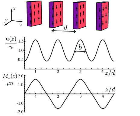
Figure 1: The uppermost panel illustrates the magnetization profile, and the lower two panels the spatial distribution along $z$-direction of the normalized number density and magnetization, Eqs. (6), in the AFSC state for $d=\sqrt{8}b$.

To seek the ground state of dipolar fermions in the strong coupling region beyond this critical line, we introduce a set of normalized basis states for particles localized in the $z$-direction, and in plane wave states in the transverse direction,

$$\phi_{\ell,\vec{q}_{\perp}}(x,y,z) = \frac{e^{-(z-d\ell)^{2}/2b^{2}}}{(\pi b^{2})^{1/4}}\frac{e^{i\vec{q}_{\perp}\cdot\vec{r}_{\perp}}}{\sqrt{V_{\perp}}}\chi_{\ell},$$ (5)

where the integer $\ell$, ranging from $-\infty$ to $+\infty$ labels the layer, $\vec{q}_{\perp}$ is the transverse momentum, $\vec{r}_{\perp}=(x,y)$, $V_{\perp}$ is the transverse two-dimensional volume, $d$ is the distance between neighboring layers, $b$ is the width of the layer, and the $\chi_{\ell}=(1,(-1)^{\ell+1})/\sqrt{2}$ are staggered spinors, with the center site, $\ell=0$, spin-down with respect to $\sigma_{x}$. We assume that the fermions are well localized in the $z$-direction, with $d\gtrsim\sqrt{2}b$, and in the AFSC ground state fill these states with all $\ell$, and $q_{\perp}$ up to the transverse Fermi momentum, $q_{F\perp}=\sqrt{4\pi nd}$.

The expectation values of the number density, $\Psi^{\dagger}\Psi$, and local magnetization, $\mu\Psi^{\dagger}\vec{\sigma}\Psi$, in the AFSC state are

$$\langle n(\vec{r}\,)\rangle = \frac{nd}{b\sqrt{\pi}}\sum_{\ell=-\infty}^{\infty}e^{-(z-d\ell)^{2}/b^{2}},$$

$$\langle{M_{x}}(\vec{r}\,)\rangle = -\frac{\mu nd}{b\sqrt{\pi}}\sum_{\ell=-\infty}^{\infty}(-1)^{\ell}e^{-(z-d\ell)^{2}/b^{2}},$$ (6)

and $\langle{M_{y}}(\vec{r}\,)\rangle=\langle{M_{z}}(\vec{r}\,)\rangle=0$. The AFSC state is indeed a layered structure in density, with staggered local magnetization, as illustrated in the middle and lower panels of Fig. 1. Using the Poisson summation formula, we can write the density and magnetization as

$$\langle n(\vec{r}\,)\rangle = n+2n\sum_{j=1}^{\infty}e^{-j^{2}\pi^{2}/\Gamma}\cos\left(2j\pi z/d\right),$$ (7)

$$\langle{M_{x}}(\vec{r}\,)\rangle \!\!\!\!\!= \!\!\!\!\!-2\mu n\sum_{j=1}^{\infty}e^{-(2j-1)^{2}\pi^{2}\!/4\Gamma}\!\cos\left\{(2j\!-\!1)\pi z/d\right\},$$

where the dimensionless localization parameter $\Gamma=(d/b)^{2}$ is the square of the ratio of the layer distance and the Gaussian width.

The energy density of the AFSC phase, ${\cal E}(\Gamma,\!\alpha)$, with $\alpha=1/8\pi ndb^{2}$, in units of the energy density of the free Fermi gas is

$$\frac{{\cal E}(\Gamma,\!\alpha)}{\frac{3}{5}n\epsilon_{F}}\! = \!\frac{10}{3(3\pi)^{2/3}}\Gamma^{1/3}\alpha^{2/3}+\frac{5}{3(3\pi)^{2/3}}\Gamma^{1/3}\alpha^{-1/3}$$

$$-\frac{20\pi}{3}\lambda_{d}\sum_{j=1}^{\infty}e^{-(2j-1)^{2}\pi^{2}\!/2\Gamma}\left\{\frac{1}{3}-F(\alpha)\right\}$$

$$\!\!+\frac{5}{6}\lambda_{s}\biggl{\{}\frac{1}{2}\!-\!\sum_{j=1}^{\infty}\bigl{[}e^{-(2j-1)^{2}\pi^{2}\!/2\Gamma}-e^{-2j^{2}\pi^{2}\!/\Gamma}\bigl{]}\!\biggl{\}}.$$

The first term on the right is the one-dimensional zero-point energy in the $z$-direction, and the second term is the two-dimensional kinetic, or Fermi, energy within a layer. We note that $2\alpha$ is the dimensionless ratio of these two terms. The third term arises from the dipole-dipole interaction, with $1/3$ and $-F(\alpha)$ the direct and exchange contributions, respectively, where

$$F(\alpha)$$

$$= \!\!\alpha\!\int_{0}^{\infty}\!{\rm d}sJ_{1}^{2}\!\left(\!\sqrt{2s/\alpha}\right)e^{s}\biggl{\{}\frac{2s+1}{s}K_{0}(s)\!-\!2K_{1}(s)\biggl{\}},$$

and $J_{i}$ and $K_{i}$ are the Bessel functions of the first kind and second kind, respectively. The final, positive, term in Eq. (LABEL:AFSC:energy) is the contribution of the contact interaction. The lowest energy AFSC state is obtained by minimizing ${\cal E}(\Gamma,\!\alpha)$ with respect to $\Gamma$ and $\alpha$ for given $\lambda_{d}$ and $\lambda_{s}$. It is sufficient to take only the $j=1$ mode in Eq. (LABEL:AFSC:energy) (one-mode approximation) to obtain the ground state energy to a few percent accuracy for $\Gamma\lesssim 10$, the regime in which particles are not too well localized in the layers. In constructing the phase diagram of the system as functions of the short range interaction, measured by $\lambda_{s}$, and the dipole-dipole interaction, measured by $\lambda_{d}$, as shown in Fig. 2, we compare the minimum ${\cal E}(\Gamma,\!\alpha)$ with the energy of the interacting Fermi gas phase [$\epsilon_{\rm FG}={\frac{3}{5}n\epsilon_{F}}\left(1+\frac{5}{12}\lambda_{s}\right)$] and with that of the fully polarized ferronematic state Fradkin:2009 ; note3 .

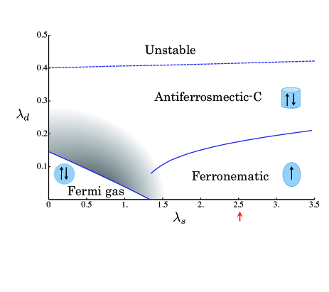
Figure 2: Schematic phase structure of dipolar fermions as a function of $\lambda_{s}$ and $\lambda_{d}$, showing the non-magnetized Fermi gas phase, the locally weakly magnetized state shown by the shaded area, the ferronematic region, and the antiferrosmectic-C region. Beyond the upper dashed line the system becomes unstable against collapse.

The resultant phase diagram, shown schematically in Fig. 2, is composed of four regions: (I) the non-magnetized Fermi gas phase (the lower left corner), which has a spherical Fermi surface with equal population of both species, (II) the AFSC phase (the upper right region) which has a cylindrical Fermi surface with equal populations of both species, (III) the ferronematic phase (the lower right region) which has a spheroidal Fermi surface with only a single species, and (IV) an unstable region. Determining the detailed structure of the intermediate locally weakly magnetized state, shown as the shaded area Sogo:2012 ; Matsui:1978 , and the question of whether this phase evolves smoothly into the AFSC phase with increasing dipole interaction strength, are interesting open problems beyond the scope of this paper.

In Fig. 3 we plot the localization parameter $\Gamma$ and the kinetic energy ratio $\alpha$ vs. $\lambda_{d}$ for $\lambda_{s}=2.5$, corresponding to the red arrow in Fig. 2. The exchange contribution of the dipole-dipole interaction in the AFSC state is of order 30% of the direct term, decreasing with increasing $\lambda_{d}$.

The different regions of the phase diagram are related as follows:

From Fermi gas to AFSC: The energy of the non-magnetized Fermi gas is increased only by the contact interaction, not by the dipolar interaction. On the other hand, the AFSC phase has a net decrease in energy from the dipolar attraction between neighboring layers, despite the increase of the fermion kinetic energy due to the spatial localization in the $z$-direction. Therefore, as $\lambda_{d}$ increases, the non-magnetized Fermi gas, after making a transition to a locally weakly magnetized phase (the shaded region in Fig. 2), passes into the AFSC phase.

From Fermi gas to ferronematic: The fully polarized ferronematic phase has only one component, and it does not experience the contact repulsion, although its Fermi energy increases in comparison to the two-component Fermi gas. Therefore, there is a transition from the Fermi gas phase to the ferronematic phase for sufficiently large $\lambda_{s}$, as long as $\lambda_{d}$ is small.

From ferronematic to AFSC: In the fully polarized ferronematic phase with small $\lambda_{d}$, the Fermi surface is deformed from spherical due to the anisotropy of the dipole interaction Sogo:2009 ; Fradkin:2009 . As $\lambda_{d}$ increases, however, the one-dimensional periodic structure emerges spontaneously, enhancing the dipolar attraction in a two-component system. This leads to a transition from weak to strong deformation of the Fermi surface, replacing the ferronematic phase by the AFSC phase for a wide range of $\lambda_{d}$.

Instability: For $\lambda_{d}$ above the dashed line in Fig. 3 ($\lambda_{d}\simeq 0.40\sim 0.43$), the AFSC phase becomes unstable due to large attraction between the layers. The dashed line is determined by the compressibility, $K^{-1}=n\partial P/\partial n=n^{2}\partial^{2}{\cal E}/\partial n^{2}$, vanishing. A similar instability of the ferronematic phase has been reported in Sogo:2009 ; Fradkin:2009 . Determining the stable states of the system above the dashed line remains a problem for future work.

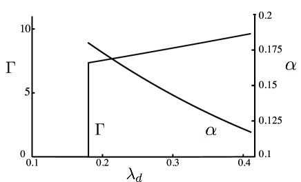
Figure 3: Optimal values of $\Gamma$ and $\alpha$ as a function of $\lambda_{d}$ for $\lambda_{s}=2.5$.

We now relate the present model to laboratory systems. Numerically, the coupling constants are $\lambda_{d}=2.7\times 10^{-3}m_{100}n_{12}^{1/3}\mu_{10}^{2}$ and $\lambda_{s}=2.6\times 10^{-2}n_{12}^{1/3}a_{10}$, where $m_{100}$ is the atomic (or molecular) mass in units of 100 proton masses, $n_{12}$ is the density in units of $10^{12}{\rm cm}^{-3}$, $\mu_{10}$ is the magnetic dipole moment in units of ${10\mu_{B}}$, and $a_{10}$ is the effective scattering length, $gm/4\pi$, in units of 10 nm. Then $\lambda_{d}/\lambda_{s}=0.1\times m_{100}\mu_{10}^{2}/a_{10}$. The distance $d$ between layers in the AFSC phase is $\sim 10^{2}n_{12}^{-1/3}$ in $\mu$m, which may be fine compared to the size of ultracold atomic gases. To reach into the AFSC phase with Dy atoms would require $n\sim 5\times 10^{17}$ cm^-3, a density which can be greatly reduced by resonantly enhancing $a$. Molecules with larger masses and magnetic moments, e.g. diatomic molecules of Dy, have larger $\lambda_{d}$ also enabling the AFSC phase to be realized at smaller density.

For dipoles with more than two internal states, the relation of diagonal and off-diagonal moments is modified, so that in Eq. (2) $\sigma_{z}$ must be replaced by diag$\{A,B\}$ where $A=\bra{\uparrow}\mu_{z}\ket{\uparrow}/\mu$, and $B=\bra{\downarrow}\mu_{z}\ket{\downarrow}/\mu$, with $\mu_{z}$ the $z$-component of the moment operator, and $\mu$ the transition moment. This correction enhances local magnetic fields along the $z$-direction, which for a system uniform in the $x$- and $y$-directions can at most be constant (and generally small compared with trapping fields).

Calculation of the finite temperature phase diagram remains an open problem. The scale of energies in the various phases at zero temperature are of order the Fermi energy, and so one expects significant structure to emerge at temperatures below the Fermi temperature. The regime of stability at finite temperature of the two-dimensional sheets in the AFSC phase in finite volume, particularly against a Landau-Peierls instability, needs to be determined. Finally, one should consider other possible phases in the system, e.g., AFSC states with population imbalance, states with structure in the sheets such as a “spaghetti phase” benjamin , and superfluid states of spin-triplet p-wave paired atoms which could emerge at large $\lambda_{d}$.

As Luttinger and Tisza Luttinger:1946 showed, the lowest energy configuration of classical dipoles on a cubic lattice has the same dipole configuration as the present AFSC phase. Thus we can reasonably expect that the AFSC state can be realized in an optical lattice and might even be enhanced when the pitch of the spontaneous localization is commensurate with that of the lattice potential.

The dipole-dipole interaction is caused by exchange of the vector potential $\vec{A}(\vec{r})$ between dipolar atoms. Therefore spatially varying magnetizations $\langle\vec{M}(\vec{r})\rangle$ in the AFSC phase correspond to the spontaneous formation of a non-zero $\langle\vec{A}(\vec{r})\rangle$, through the Maxwell equation: $\nabla^{2}\langle\vec{A}(\vec{r})\rangle=-4\pi\nabla\times\langle\vec{M}(\vec{r})\rangle$. Very similar meson condensed states have been proposed in nuclear physics where the $\rho$-meson in nuclear matter corresponds to $\vec{A}(\vec{r})$ for magnetic dipolar atoms, and the $\pi$-meso corresponds to the scalar potential $A_{0}(\vec{r})$ for electric dipolar atoms. Such a correspondence may open the interesting future possibility of learning properties of states of dense matter inside neutron stars via cold atom experiments in the laboratory.

- (1) Reviewed in M. A. Baranov, Phys. Rep. 464, 71 (2008).
- (2) M. Lu, S. H. Youn and B. L. Lev, Phys. Rev. Lett. 104, 063001 (2010).
- (3) M. Lu, N. Q. Burdick, and B. L. Lev, Phys. Rev. Lett. 108, 215301 (2012).
- (4) See, e.g., B. Lian, T.-L. Ho, and H. Zhai, Phys. Rev. A 85, 051606(R) (2012).
- (5) T. Sogo, L. He, T. Miyakawa, S. Yi, H. Lu and H. Pu, New J. Phys. 11, 055017 (2009).
- (6) B. M. Fregoso and E. Fradkin, Phys. Rev. Lett. 103, 205301 (2009).
- (7) B. M. Fregoso, K, Sun, E. Fradkin, and B. L. Lev, New J. of Phys. 11, 103003 (2009).
- (8) Y. Yamaguchi, T. Sogo, T. Ito and T. Miyakawa, Phys. Rev. A 82, 013643 (2010); K. Sun, C. Wu and S. D. Sarma, Phys. Rev. B 82, 075105 (2010).
- (9) T. Sogo, M. Urban, P. Schuck and T. Miyakawa, Phys. Rev. A 85, 031601(R) (2012).
- (10) J. M. Luttinger and L. Tisza, Phys. Rev. 70, 954 (1946).
- (11) T. Kunihiro, Prog. Theor. Phys. 60, 1229 (1978).
- (12) T. Matsui, K. Sakai, M. Yasuno, Prog. Theor. Phys. 60, 442 (1978); ibid. 61, 1093 (1979).
- (13) Reviewed in G. Baym and D. K. Campbell, in Mesons in Nuclei, ed. M. Rho and D. Wilkinson (North Holland, Amsterdam, 1979); A. B. Migdal et al., Phys. Rep. 192, 179 (1990).
- (14) R. Tamagaki et al., Prog. Theor. Phys. Suppl. 112, 1 (1993).
- (15) P. M. Chaikin and T. C. Lubensky, Principles of condensed matter physics (Cambridge Univ. Press, 1995).
- (16) This ordering is reminiscent of the smectic-C type structure in liquid crystals. Note that a smectic-A structure with leads to dipole-dipole repulsion between neighboring sheets and is not favored.
- (17) In general, the dipole moment is different for terms diagonal and off-diagonal in “spin”; the relevant interaction here is the transition between the two spin states, and thus is the transition spin magnetic moment. For example, in 163Dy the transition moment from the to the state is the ratio of off-diagonal to diagonal Clebsch-Gordan coefficients, , times the atomic magnetic moment, 10, or 4.26.
- (18) We do not consider here the partially polarized ferronematic state discussed in Fradkin:2009 , which occupies only a small region of the phase diagram.
- (19) B. Fregoso, private communication to G. Baym.