Exotic quantum statistics of composite particles and frustrated quasiparticles

Abstract

We study the exotic quantum statistical behavior of composite particle of double-spin cluster and quasiparticle of triple-spin cluster in a four-spin quantum model. We constructed a four spin-1/2 model on a triangular star lattice but added frustrated coupling terms of plaquette quasiparticles. The eigenstates of this model are maximal entangled quantum states like Greenberger-Horne-Zeilinger state and Yeo-Chua’s genuine four-qubit entangled state. We generalized the conventional definition for quantum statistics of two elementary particles to composite particle of multispin clusters. Greenberger-Horne-Zeilinger state and Yeo-Chua’s genuine four-qubit entangled state showed different behavior according to this generalized definition. The quantum statistical behavior of the composite particle of double-spin cluster is neither boson nor fermion in ground state and some intermediate excited states. The triple-spin cluster of this model is eigen-quasiparticles. We perform permutation operation on the eigenstates of triple-spin plaquette operator according to this generalized definition for quantum statistics of multi-spin clusters, the statistical matrix of exchanging two triple-spin quasiparticles is far beyond fermion and boson. The von Neumann entropy of the triple-spin quasiparticle is also highly nontrivial. These nontrivial quantum statistical behavior of plaquette quasiparticles is helpful for decoding the non-abelian anyons in Kitaev honeycomb model.

I Introduction

Fermion is the most fundamental building block for matters. Most bosons are composite particle of even number of fermions. The typical fermion, proton, is also a composite particle of three quarks. The collective wave function of two fermions is anti-symmetric, $\psi(r_{1},r_{2})=-\psi(r_{2},r_{1})$. While the collective wave function of two bosons is symmetric, $\psi(r_{1},r_{2})=\psi(r_{2},r_{1})$. The statistical factor of anyon is defined as $\psi(r_{1},r_{2})=e^{i\theta}\psi(r_{2},r_{1})$, where [$\theta=\alpha\pi$,$1<\alpha<2$]. Different statistical behavior of these composite particles leads to different physical phenomena. The unknown statistical behavior of composite particles gained long-lasting research interest until today. One recent study defines an arbitrary composite boson by the product of two fermion or boson operator sylee , interesting eigenstate and commutator was derived by defining an effective composite boson annihilation operator sylee . If Pauli principle has no influence on physical behavior of many composite bosons, the composite boson of two entangled fermions can be treated as an elementary bosonic particle Tichy . The upper and lower bounds of a defined quantity determines the bosonic statistical behavior of a pair of entangled fermions Chudzicki . Many composite particles in strongly correlated quantum many body system exhibits exotic statistical behavior beyond boson and fermion, such as quasiparticle and quasiholes in fractional quantum Hall system Laughlin , abelian anyon model for topological quantum computation Nayak , and so on. The non-abelian plaquette excitations in Kitaev’s honeycomb model obeys non-trivial topological fusion rule. However it is hard to find the exact relationship between the topological fusion rule and the conventional textbook definition of anyons above. In this paper, we proposed a generalized definition of the textbook’s definition of anyon for studying the composite particle of double-spins and triple-spin quasiparticles in a triangular star model with frustrated quasiparticle, which can be viewed as the minimal model of Kitaev honeycomb model kitaev , but the additionally introduced frustration terms makes it more complicate than Kitaev honeycomb model.

It is the quantum entanglement between the elementary particles of a composite particle that drives the statistical behavior of composite particle out of the scope of boson and fermion. Quantum entanglement attracted many research interests for quantum computation Horodecki Nest . The upper bounds of squared concurrence CJZhang and its dual lower bound of squared concurrence for arbitrary mixed state Mintert can be used to estimate the entanglement in experimental measurement. Modern quantum optical technology can implement finite number of qubits pan . Greenberger-Horne-Zeilinger state has been generated in laboratory GHZstate , so did the W-state of four qubits Wstate . The Cross-Kerr nonlinearity of quantum optics zhao is suggested for implementing Yeo-Chua’s genuine four-qubit entangled states yeo . Since the four-qubit states is very convenient for experiment implementation, theoretical research interest on quantum entanglement of four-qubit state is accumulating rapidly Horodecki .

Recently the classification of quantum entangled states by symmetry has aroused many research interest Vladislav Aulbach Migda Jeong wang Markham . Entangled state is categorized by the permutation symmetry of the subsystems Aulbach . the Greenberger-Horne-Zeilinger-Like symmetric state of four qubits is constructed By extending the symmetry of three-qubit Greenberger-Horne-Zeilinger (GHZ) state to four qubits Jeong . While most of these states is constructed without Hamiltonian. In this triangular model, we actually derived many entangled states by directly solving this four-spin quantum model. We generalize the textbook definition of permutating two particles in collective wave function to permutating two pairs of particles, and also generalize it to permutating two composite quasiparticle of three-spin cluster. With the help of Hamiltonian operator and plaquette operator, we found the generalized triplet state and singlet state of the composite spin of double-spins.

This four-spin model is inspired by Kitaev honeycomb lattice model for topological quantum computation kitaev Nayak . We built the coupled four spin model on a triangular star lattice. The first part of the Hamiltonian obeys the coupling rule of Kitaev honeycomb model kitaev . The newly added second part is anti-ferromagnetic coupling between neighboring plaquette operators which sits right at the center of plaquette. The anti-ferromagnetic coupling between particles on triangular lattice results in geometrically frustrated quantum system Moessner . The geometric frustration between plaquette quasiparticles of this four-spin model also introduced interesting statistics of quasiparticles beyond that of Kitaev honeycomb model, for instance, the ground state is no longer homogeneous gauge pattern.

The article is organized as following: In section II, we proposed the triangular star model and the generalized definition for statistics of composite particle of double-spins. The nontrivial statistical matrix of composite particle of double-spins was computed. In section III, we computed the quantum statistical matrix of the plaquette quasiparticle of triple-spin clusters. A non-trivial statistical matrix and von Neumann entropy was found. Section IV is a brief summary.

II The quantum statistics of composite double-spin operators in a triangular star model

This triangular star model places the four particles at the vertices of a triangular star lattice(Fig. 1). The triangular star has three independent triangular plaquette. The four particles coupled to each other following Kitaev honeycomb model. We added an antiferromagnetic coupling between the nearest neighboring plaquette on the Hamiltonian,

$$H_{a} = J_{x}\sigma^{x}_{1}\sigma^{x}_{3}+J_{y}\sigma^{y}_{1}\sigma^{y}_{2}+J_{z}\sigma^{z}_{2}\sigma^{z}_{3}+J_{x}\sigma^{x}_{2}\sigma^{x}_{4}+J_{y}\sigma^{y}_{3}\sigma^{y}_{4}$$ (1)

$$+ J_{z}\sigma^{z}_{1}\sigma^{z}_{4}+J_{p}\hat{S}_{\textbf{1}}\hat{S}_{\textbf{2}}+J_{p}\hat{S}_{\textbf{2}}\hat{S}_{\textbf{3}}+J_{p}\hat{S}_{\textbf{3}}\hat{S}_{\textbf{1}}.$$

$\begin{array}[]{c@{\hspace{0.15in}}c}\includegraphics[scale={0.23}]{four.eps}\hfil\hskip 10.84006pt&\includegraphics[scale={0.20}]{levels.eps}\\ \mbox{\bf(a)}\hfil\hskip 10.84006pt&\mbox{\bf(b)}\end{array}$

Figure 1: (a) The triangular star model. Quasiparticle sits right at the center of each triangle. (b) The eigenenergy levels of the triangular star model with respect to the parameter setting of $(J_{p}=2J_{x},\;J_{z}=2J_{x},\;J_{y}=2J_{x})$.

The three plaquette operators $\hat{S}_{\textbf{j}}$ are quantum string operators around each triangular plaquette,

$$\hat{S}_{\textbf{1}}=\sigma^{z}_{1}\sigma^{x}_{2}\sigma^{y}_{3},\;\;\hat{S}_{\textbf{2}}=\sigma^{z}_{4}\sigma^{y}_{2}\sigma^{x}_{3},\;\;\hat{S}_{\textbf{3}}=\sigma^{x}_{1}\sigma^{z}_{2}\sigma^{y}_{4}.\;\;$$ (2)

They commute with Hamiltonian and commute with each other, i.e., $[\hat{S}_{\textbf{i}},H]=0$, $[\hat{S}_{\textbf{i}},\hat{S}_{\textbf{j}}]=0,\;i\neq{j}=1,2,3$.

The three conserved plaquette operator divide the total Hilbert space into three sectors. Each plaquette operator has eigenvalues $+1$ and $-1$ within its Hilbert space, $\hat{S}_{\alpha}|\psi\rangle=\pm 1|\psi\rangle$. Every triangular plaquette operator defines an effective Ising spin within each sector. In the Kitaev honeycomb model, the ground state chooses a homogeneous gauge pattern. All plaquette operators take the same eigenvalue. As there is antiferromagnetic coupling between two plaquette, the ground state is no longer the homogeneous gauge pattern. The ground state bear the frustrated gauge pattern.

We first solve the model by diagonalizing the Hamiltonian matrix. The spin operators take a sixteen dimensional representation,

$$\sigma^{\mu}_{1} = \hat{\sigma}^{\mu}_{1}\otimes{\textbf{I}_{2}}\otimes{\textbf{I}_{3}}\otimes{\textbf{I}_{4}},\;\;\;\sigma^{\mu}_{2}={\textbf{I}_{1}}\otimes\hat{\sigma}^{\mu}_{2}\otimes{\textbf{I}_{3}}\otimes{\textbf{I}_{4}},$$

$$\sigma^{\mu}_{3} = {\textbf{I}_{1}}\otimes{\textbf{I}_{2}}\otimes\hat{\sigma}^{\mu}_{3}\otimes{\textbf{I}_{4}},\;\;\;\sigma^{\mu}_{4}={\textbf{I}_{1}}\otimes{\textbf{I}_{2}}\otimes{\textbf{I}_{3}}\otimes\hat{\sigma}^{\mu}_{4},\;\;\;$$ (3)

where $\hat{\sigma}^{\mu}_{i}$ are the conventional Pauli matrices and ${\textbf{I}_{i}}$ is the 2$\times$2 identity matrix. The symbol $\otimes$ denotes direct product. The eigenvalues of the sixteen dimensional Hamiltonian matrix lead to eight discrete energy levels,

$$E^{\pm}_{p} = 3J_{p}\pm 2\sqrt{J^{2}_{x}+J^{2}_{y}+J^{2}_{z}},\;\;$$

$$E^{\pm}_{\mu} = -J_{p}\pm 2J_{\mu},\;\;\;\;\;\mu=x,y,z.$$ (4)

Each energy level has two fold degeneracy. The energy levels are listed in Fig. 1 (b). The eigenenergy and eigenstates are computed directly from the Hamiltonian matrix. The newly added coupling terms of two plaquette operators commute with Hamiltonian. It does not modify the physics mechanism of Kitaev honeycomb model. The vortex excitation in the triangular plaquette represents the same type of quasiparticle excitation of Kitaev honeycomb model. The main different character of this triangle star model from Kitaev honeycomb model is the neighboring quasiparticles are now antiferromagnetically coupled to each other. As the three plaquette are placed on a triangle, it forms a typical pattern of frustrated Ising spin system. If the three quasiparticles have the same eigenvalue, it is a fully frustrated system since the spins intend to be parallel to each other. If there is only one pair of spin are oriented at the same direction, it is the minimally frustrated state. The ground state is the minimally frustrated quasiparticle state for which the system bears minimal energy.

The two levels with higher eigenenergy $E^{\pm}_{p}$ correspond to excited states for which the eigenvalues of the three plaquette operators takes the same value ${S}_{\textbf{1}}={S}_{\textbf{2}}={S}_{\textbf{3}}=\pm 1$. The three pairs of energy level with lower energy $E^{\pm}_{\mu}$ correspond to the frustrated gauge pattern. Only one pair of quasiparticles is not frustrated for $E^{\pm}_{p}$. If $J_{x}=J_{y}=J_{z}$, the six energy levels of $E^{\pm}_{\mu}$ would be degenerated.

If the quasiparticle coupling interaction $J_{p}$ becomes zero, the triangular star model reduces to a finite Kitaev honeycomb model on triangular star lattice. For a stronger quasiparticle coupling interaction than the spin coupling,

$$J_{p}=2J_{x},\;\;\;J_{z}=2J_{x},\;\;\;J_{y}=2J_{x},$$ (5)

there exists four degenerated states with zero energy. Without losing important physics, we focus on this special parameter setting of Eq. (5) in the following. By representing the eigenvectors of the 16 dimensional Hamiltonian matrix by the 16 four-spin basis, we derived the spin configurations corresponding to the four zero energy states,

$$|o\rangle_{1} = \frac{1}{2\sqrt{15}}[|\Uparrow\Uparrow\rangle+|\Downarrow\Downarrow\rangle+2|\circlearrowright\circlearrowleft\rangle+2|\circlearrowleft\circlearrowright\rangle$$

$$- 5|\circlearrowleft\circlearrowleft\rangle-5|\circlearrowright\circlearrowright\rangle],$$

$$|o\rangle_{2} = \frac{1}{2}[|\Uparrow\circlearrowright\rangle+|\circlearrowright\Uparrow\rangle+|\circlearrowleft\Downarrow\rangle+|\Downarrow\circlearrowleft\rangle],$$

$$|o\rangle_{3} = \frac{1}{2}[|\Uparrow\circlearrowleft\rangle+|\circlearrowright\Downarrow\rangle+|\circlearrowleft\Uparrow\rangle+|\Downarrow\circlearrowright\rangle],$$

$$|o\rangle_{4} = \frac{1}{2\sqrt{3}}[|\Uparrow\Downarrow\rangle+|\Downarrow\Uparrow\rangle+2|\circlearrowleft\circlearrowleft\rangle+2|\circlearrowright\circlearrowright\rangle$$ (6)

$$- |\circlearrowright\circlearrowleft\rangle-|\circlearrowleft\circlearrowright\rangle].$$

Here the symbols in the quantum wave function represent the double spin configurations,

$$|\Uparrow\rangle=|\uparrow\uparrow\rangle,\;|\Downarrow\rangle=|\downarrow\downarrow\rangle,\;|\circlearrowright\rangle=|\uparrow\downarrow\rangle,\;|\circlearrowleft\rangle=|\downarrow\uparrow\rangle.$$ (7)

The eigenenergy of the states above is zero, i.e., $H|o\rangle_{\mu}=0,\;\;\mu=1,2,3,4.$ The zero energy state pair of $|o\rangle_{2}$ and $|o\rangle_{3}$ comes from the minimal frustrated gauge pattern, i.e, $E^{+}_{x}=-J_{p}+2J_{x}=0$. The two zero energy states of $|o\rangle_{1}$ and $|o\rangle_{4}$ correspond to the fully frustrated states $E^{-}_{p}=3J_{p}-6J_{x}=0$.

The ground state has four fold degeneracy. We denote them as $|g\rangle_{\mu},\;\;\mu=1,2,3,4.$,

$$|g\rangle_{1}=\frac{1}{2}[|\Downarrow\circlearrowleft\rangle-|\Uparrow\circlearrowright\rangle+|\Uparrow\circlearrowleft\rangle-|\Downarrow\circlearrowright\rangle],$$

$$|g\rangle_{2}=\frac{1}{\sqrt{2}}[|\Downarrow\Uparrow\rangle-|\Uparrow\Downarrow\rangle],$$

$$|g\rangle_{3}=\frac{1}{{2}}[|\circlearrowleft\Uparrow\rangle-|\circlearrowright\Downarrow\rangle+|\circlearrowleft\Downarrow\rangle-|\circlearrowright\Uparrow\rangle],$$

$$|g\rangle_{4}=\frac{1}{\sqrt{2}}[|\circlearrowleft\circlearrowleft\rangle-|\circlearrowright\circlearrowright\rangle].$$ (8)

The eigenenergy of the four ground states are $E_{g}=-6J_{x}$, i.e., $\;H|g\rangle_{\mu}=-6J_{x}|g\rangle_{\mu},\;\;\mu=1,2,3,4.$ The ground states are the minimally frustrated quasiparticle states. Two of them comes from $E^{-}_{y}=-J_{p}-2J_{y}=-6J_{x}$. The other two states is for $E^{-}_{z}=-J_{p}-2J_{z}=-6J_{x}$. The spin configuration of the two states $|g\rangle_{1}$ and $|g\rangle_{3}$ is the superposition of three-up-one-down state and three-down-one-up state. The two states of $|g\rangle_{2}$ and $|g\rangle_{4}$ is the superposition state of four spin basis with two-up spins and two-down spins. If we flip the spins of all of the four ground states, it generates a minus sign upon the original wave function. So the ground state breaks $Z_{2}$ symmetry.

The whole Hilbert space of eigenstates can be classified into two classes. The first class breaks the $Z_{2}$ symmetry. This class only includes the ground state and the four degenerated states with respect to $2J_{x}$. The other class keeps $Z_{2}$ symmetry. This class includes the zero energy states, the highest excited states and all the rest excited states.

The energy level $\omega=12J_{x}$ is the highest energy level corresponding to the fully frustrated quasiparticle state. The spin configuration corresponding to this two-fold degenerated level is $|e\rangle_{15}$ and $|e\rangle_{16}$,

$$|e\rangle_{15} = \frac{1}{2\sqrt{3}}[|\Uparrow\Uparrow\rangle+|\Downarrow\Downarrow\rangle+2|\circlearrowright\circlearrowleft\rangle+2|\circlearrowleft\circlearrowright\rangle$$

$$+ |\circlearrowleft\circlearrowleft\rangle+|\circlearrowright\circlearrowright\rangle],$$

$$|e\rangle_{16} = \frac{1}{2\sqrt{15}}[|\Uparrow\Downarrow\rangle+|\Downarrow\Uparrow\rangle+2|\circlearrowright\circlearrowright\rangle+2|\circlearrowleft\circlearrowleft\rangle$$ (9)

$$+ 5|\circlearrowleft\circlearrowright\rangle+5|\circlearrowright\circlearrowleft\rangle],$$

The eigenstates of this model can be viewed as entangled quantum states of two double-spin clusters. For example, the nearest excited state above the zero energy state has four-fold degeneracy. The spin configuration of the four states are

$$|e\rangle_{11} = \frac{1}{\sqrt{2}}[-|\Uparrow\Uparrow\rangle+|\Downarrow\Downarrow\rangle],$$

$$|e\rangle_{12} = \frac{1}{2}[-|\Uparrow\circlearrowright\rangle-|\Uparrow\circlearrowleft\rangle+|\Downarrow\circlearrowright\rangle+|\Downarrow\circlearrowleft\rangle],$$

$$|e\rangle_{13} = \frac{1}{2}[-|\circlearrowright\Uparrow\rangle+|\circlearrowright\Downarrow\rangle-|\circlearrowleft\Uparrow\rangle+|\circlearrowleft\Downarrow\rangle],$$

$$|e\rangle_{14} = \frac{1}{\sqrt{2}}[-|\circlearrowright\circlearrowleft\rangle+|\circlearrowleft\circlearrowright\rangle].$$ (10)

The corresponding eigenenergy with respect to $\{|e\rangle_{11}$, $|e\rangle_{12}$, $|e\rangle_{13}$, $|e\rangle_{14}\}$ is $E=2J_{x}$. The spin configurations of $|e\rangle_{12}$ and $|e\rangle_{13}$ is the superposition of three-up-one-down and three-down-one-up. The state $|e\rangle_{11}$ can be viewed as a dual state of the well-known Greenberger-Horne- Zeilinger state for four qubit GHZstate ,

$$|GHZ\rangle=|\Uparrow\Uparrow\rangle+|\Downarrow\Downarrow\rangle.$$ (11)

$|e\rangle_{14}$ is a singlet pair state of two double-spin clusters . The other two states, $|e\rangle_{12}$ and $|e\rangle_{13}$, can be viewed as generalized W-state of four qubits Wstate ,

$$|W\rangle=(|\Uparrow\circlearrowright\rangle+|\Uparrow\circlearrowleft\rangle+|\circlearrowright\Uparrow\rangle+|\circlearrowleft\Uparrow\rangle).$$ (12)

The two degenerated states of energy level $E=-4J_{x}$ are $|e\rangle_{9}\}$ and $\{|e\rangle_{10}$, they both bear similar state structure as W-state,

$$|e\rangle_{9} = \frac{1}{{2}}[|\Uparrow\circlearrowright\rangle-|\circlearrowright\Uparrow\rangle-|\circlearrowleft\Downarrow\rangle+|\Downarrow\circlearrowleft\rangle],$$

$$|e\rangle_{10} = \frac{1}{{2}}[|\Uparrow\circlearrowleft\rangle-|\circlearrowleft\Uparrow\rangle-|\circlearrowright\Downarrow\rangle+|\Downarrow\circlearrowright\rangle].$$ (13)

These eigenstates are genuine entangled states of four spins. The zero energy states and highest excited states, $\{|o\rangle_{1}$, $|o\rangle_{4}\}$ and $\{|e\rangle_{15}$, $|e\rangle_{16}\}$, can be classified into the same class as Yeo-Chua’s genuine four-qubit entangled state yeo ,

$$|\chi^{00}\rangle = |\Downarrow\Downarrow\rangle-|\Downarrow\Uparrow\rangle-|\circlearrowleft\circlearrowleft\rangle+|\circlearrowleft\circlearrowright\rangle$$ (14)

$$+ |\circlearrowright\circlearrowleft\rangle+|\circlearrowright\circlearrowright\rangle+|\Uparrow\Downarrow\rangle+|\Uparrow\Uparrow\rangle.$$

The eigenstates of this model can be implemented by the same operation as that for generating Yeo-Chua’s genuine four-qubit entangled state using cross-Kerr nonlinearity zhao . These states can be mapped into graph states following the strategy of Ref. ye , the observable operators in graph state theory has a physical meaning in this quantum model. Usually Yeo-Chua’s genuine four-qubit entangled state or W-state is constructed without a Hamiltonian, but here we can derive the eigenenergy of these states. One can decompose an arbitrary entangled state as the superposition of these eigenstates. The weight of each eigenstate is marked by its eigenvalue. This offers us a new angle to see the internal structure of the quantum entanglement.

The Wootters’s concurrence provide a convenient way to quantify quantum entanglement of two-qubit states Wootters ,

$$\tau_{abcd}=|\langle\psi|\hat{\sigma}^{y}_{a}\otimes{\hat{\sigma}^{y}_{b}}\otimes{\hat{\sigma}^{y}_{c}}\otimes{\hat{\sigma}^{y}_{d}}|\psi^{\ast}\rangle|^{2}.$$ (15)

This concurrence has a physical interpretation in this quantum model since none of the eignestates here includes complex numbers. The concurrence operator corresponds to conserved plaquette operator in this triangular star model. The product of any two plaquette operators is a string of four identical spin operators,

$$\hat{S}_{\textbf{1}}\hat{S}_{\textbf{2}} = \sigma^{z}_{1}\sigma^{z}_{2}\sigma^{z}_{3}\sigma^{z}_{4},\;\ \hat{S}_{\textbf{2}}\hat{S}_{\textbf{3}}=\sigma^{x}_{1}\sigma^{x}_{2}\sigma^{x}_{4}\sigma^{x}_{3},$$

$$\hat{S}_{\textbf{3}}\hat{S}_{\textbf{1}} = \sigma^{y}_{1}\sigma^{y}_{2}\sigma^{y}_{3}\sigma^{y}_{4}.\;\;$$ (16)

The plaquette operators keep an arbitrary ground state vector within ground state. For example, the operation of plaquette operator $\hat{S}_{\textbf{1}}$ on the vector ground state, $\Psi_{[g_{1234}]}=[\;|g\rangle_{1},\;|g\rangle_{2}\;,|g\rangle_{3}\;,|g\rangle_{4}\;]^{T},$ gives a matrix,

$$\hat{S}_{\textbf{1}}\Psi_{[g_{1234}]}=\left[\begin{array}[]{cccc}0&0&i&0\\ 0&0&0&-i\\ -i&0&0&0\\ 0&i&0&0\\ \end{array}\right]\left[\begin{array}[]{c}|g\rangle_{1}\\ |g\rangle_{2}\\ |g\rangle_{3}\\ |g\rangle_{4}\\ \end{array}\right].$$ (25)

The operation of concurrence operator reads, $\hat{\tau}=\hat{S}_{\textbf{3}}\hat{S}_{\textbf{1}}$,

$$\hat{\tau}\Psi_{[g_{1234}]}=\left[\begin{array}[]{cccc}-1&0&0&0\\ 0&1&0&0\\ 0&0&-1&0\\ 0&0&0&1\\ \end{array}\right]\left[\begin{array}[]{c}|g\rangle_{1}\\ |g\rangle_{2}\\ |g\rangle_{3}\\ |g\rangle_{4}\\ \end{array}\right].$$ (34)

The four degenerated ground state are entangled states of four qubits. Since the concurrence operator now happened to be a physical observable, quantum entanglement maybe can be directly read out in experiment.

The textbook definition on quantum statistics of two indistinguishable particles starts from swapping the positions of the two particles, $\hat{P}\psi(r_{1},r_{2})=e^{i\theta}\psi(r_{2},r_{1})$, where $\theta$ is called a statistical angle and $\hat{P}$ is the exchange operator. $\theta=2\pi$ defines Boson, $\theta=\pi$ defines Fermion, while [$\theta=\alpha\pi$,$1<\alpha<2$] defines anyon.

Kitaev honeycomb model Hamiltonian can be equivalently mapped into a p-wave pairing Hamiltonian kitaev feng Nayak . This triangular star model can also transform into a fermion pairing model by inverse Jordan-Wigner transformation. Like the Cooper pair in BCS model, two spins in this model behaves as typical composite boson as that defined in Ref.sylee . While we define the composite Boson by spin operators,

$$d_{1}=\hat{\sigma}^{z}_{i}\hat{\sigma}^{z}_{j},\;\;\;d_{2}=\hat{\sigma}^{z}_{k}\hat{\sigma}^{z}_{l},\;\;\;(i\neq j\neq k\neq l).$$ (35)

These two composite Boson fulfills the Bosonic commutator $[d_{1},d_{2}]=0$. The spin operators in the composite Boson can also mapped into a string operator of fermion by Jordan-Wigner transformation feng . That kind of composite particle only exist in quantum many body system on lattice. Here we shall put the triangular star model equivalently on a one dimensional small lattice.

As all know, switching two fermions would generate a negative sign in front of the collective wave function. A composite particle composed of two fermions has complicate behaviorsylee . Here the composite particle of two spins also demonstrate complicate statistical behavior beyond Boson. We define a permutation operator $P[{12;34}]$,

$$P[{12;34}]\Psi(1234)=\Psi(3412)=\eta\Psi(1234).\;\;$$ (36)

Conventionally if $\eta=+1$, we call the composite particle as a Boson. The Composite particle is fermion if $\eta=-1$. If $\eta$ bear more complex structure, we might call the composite particle as exotic composite particles. These permutation operator plays a similar role as the braiding operator in fraction quantum Hall system Nayak . In the quantum Hall system, the wave function is Laughlin wave function, while the labels, ”1,2,3,4”, denote the position of quasiparticles or quasi-holes. Applying this permutation operator on the well-known Greenberger-Horne- Zeilinger state GHZstate shows it is symmetric state of double qubit,

$$P[{12;34}]|GHZ\rangle=|\Uparrow\Uparrow\rangle+|\Downarrow\Downarrow\rangle=|GHZ\rangle.$$ (37)

While the generalized W-state of four qubits Wstate is also symmetric state of double qubit,

$$P[{12;34}]|W\rangle=|\Uparrow\circlearrowright\rangle+|\Uparrow\circlearrowleft\rangle+|\circlearrowright\Uparrow\rangle+|\circlearrowleft\Uparrow\rangle=|W\rangle.$$ (38)

But Yeo-Chua’s genuine four-qubit entangled state yeo has complicate behavior under the operation of this permutation operator. We decompose Yeo-Chua’s state as the sum of two parts, $|\chi^{00}\rangle=|\chi_{1}^{00}\rangle+|\chi_{2}^{00}\rangle$,

$$|\chi_{1}^{00}\rangle = |\Downarrow\Downarrow\rangle+|\Uparrow\Uparrow\rangle+|\circlearrowright\circlearrowright\rangle-|\circlearrowleft\circlearrowleft\rangle+|\circlearrowleft\circlearrowright\rangle+|\circlearrowright\circlearrowleft\rangle,$$

$$|\chi_{2}^{00}\rangle = |\Uparrow\Downarrow\rangle-|\Downarrow\Uparrow\rangle.$$ (39)

The first part is symmetric of double qubit cluster, while the second part is anti-symmetric state of double qubit cluster,

$$P[{12;34}]|\chi_{1}^{00}\rangle=|\chi_{1}^{00}\rangle,\;\;\;P[{12;34}]|\chi_{2}^{00}\rangle=-|\chi_{2}^{00}\rangle.$$ (40)

The permutation operator reveals some fine property of entangled many qubit state. In this triangular star model, even if the four states bear the same eigenenergy, their behavior under the permutation operator is completely different.

The eigenstates of this model was expanded in the Hilbert space of the product operator of composite particle, $d_{1}d_{2}={\sigma}^{z}_{i}{\sigma}^{z}_{j}{\sigma}^{z}_{k}{\sigma}^{z}_{l}$. The four degenerated ground states include one femionic cluster state and one bosonic cluster states,

$$P[{12;34}]|g\rangle_{2}=(-1)|g\rangle_{2},\;\;P[{12;34}]|g\rangle_{4}=(+1)|g\rangle_{4}.$$ (41)

The rest two ground states can map into each other by the permutation operator,

$$P[{12;34}]|g\rangle_{1}=|g\rangle_{3},\;\;\;\;\;P[{12;34}]|g\rangle_{3}=|g\rangle_{1}.$$ (42)

So we define a four dimensional vector of ground cluster state,

$$\Psi_{[g_{(1234)}]}=[\;|g\rangle_{1},\;|g\rangle_{2}\;,|g\rangle_{3}\;,|g\rangle_{4}\;]^{T},$$ (43)

then the permutation operates on the vector states,

$$P[{12;34}]\Psi_{[g_{(1234)}]}=\left[\begin{array}[]{cccc}0&0&1&0\\ 0&-1&0&0\\ 1&0&0&0\\ 0&0&0&1\\ \end{array}\right]\left[\begin{array}[]{c}|g\rangle_{1}\\ |g\rangle_{2}\\ |g\rangle_{3}\\ |g\rangle_{4}\\ \end{array}\right].$$ (52)

If we select two states out of the four ground states as basis for quantum computation, the statistical factor of $\Psi_{[g_{1},g_{3}]}=[\;|g\rangle_{1},\;|g\rangle_{3}\;]^{T}$ is a Pauli matrix

$$\eta^{g13}_{{}_{[{12;34}]}}=\sigma^{x}.$$ (53)

For the other vector wave function of $\Psi_{[g_{2},g_{4}]}=[\;|g\rangle_{2},\;|g\rangle_{4}\;]^{T},$ the statistical factor of $\Psi_{[g_{2},g_{4}]}$ is another Pauli matrix

$$\eta^{g24}_{{}_{[{12;34}]}}=\sigma^{z}.$$ (54)

The statistical property of the nearest excited state above zero energy is similar to ground state,

$$P[{12;34}]|e\rangle_{11} = |e\rangle_{11},\;\;\;P[{12;34}]|e\rangle_{14}=-|e\rangle_{14}.$$

$$P[{12;34}]|e\rangle_{12} = |e\rangle_{13},\;\;\;P[{12;34}]|e\rangle_{13}=|e\rangle_{12}.$$ (55)

The four degenerate zero energy states and the highest excited states are all bosonic cluster states,

$$P[{12;34}]|o\rangle_{i} = |o\rangle_{i},\;\;i=1,2,3,4;$$

$$P[{12;34}]|e\rangle_{j} = |e\rangle_{j},\;\;j=15,16.$$ (56)

Their corresponding statistical factor are

$$\eta^{o}_{{}_{[{12;34}]}}=1,\;\;\;\;\;\eta^{15}_{{}_{[{12;34}]}}=1.$$ (57)

The first excited state has two degenerated states. Permutating two clusters produce a statistical factor beyond boson and fermions,

$$P[{12;34}]|e\rangle_{9} = e^{i\pi}[\sigma^{x}_{3}\sigma^{x}_{4}]|e\rangle_{10},\;\;$$

$$P[{12;34}]|e\rangle_{10} = e^{i\pi}[\sigma^{x}_{3}\sigma^{x}_{4}]|e\rangle_{9},$$ (58)

For the vector wave function of the first excited states, $\Psi_{[e_{9},e_{10}]}=[\;|e\rangle_{9},\;|e\rangle_{10}\;]^{T},$ the statistical factor of double spin clusters is

$$\eta^{e9}_{{}_{[{12;34}]}}=e^{i\pi}\sigma^{x}_{3}\sigma^{x}_{4}\left[\begin{array}[]{cc}0&1\\ 1&0\\ \end{array}\right].$$ (61)

As all know, logic gate operator in quantum computation can be expanded by Pauli spin matrices. Here the permutation operator of composite double spins provides one way of implementing quantum logic gate.

III The exotic quantum statistics of frustrated plaquette quasiparticle

Kitaev honeycomb model was first solved by representing a spin operator by two Majorana fermions kitaev . Later on, a further study was carried out by Jordan-Wigner transformation feng . Here we use the inverse representation of Jordan-Wigner transformation to formulate the Majorana fermion operators by spin operators yu . This inverse Jordan-Wigner transformation fulfills the commutator of fermions as that in the generalized Jordan-Wigner transformation Batista . Here we made a further mapping from fermion into Majorana fermion.

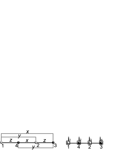
Figure 2: The one dimensional scheme of the triangular star model. The initial spatial ordering of the four particle is [1423]. The coupling bonds connecting the four particles remain the same as the original triangular star model.

The explicit formulation of inverse Jordan-Wigner transformation depends on the spatial order of the four particles. We squeeze the triangular star lattice to a one dimensional chain by keeping the topology of interacting bonds invariant. The indices $(^{\prime}1^{\prime},^{\prime}2^{\prime},^{\prime}3^{\prime},^{\prime}4^{\prime})$ in the Hamiltonian Eq. (1) are the name of the four particles instead of its spatial ordering in the one dimensional chain. We denote the four spatial positions along the one dimensional chain as $(\textbf{i}_{1}<\textbf{i}_{2}<\textbf{i}_{3}<\textbf{i}_{4})$(Fig. 2). If we place particle ${}^{\prime}1^{\prime}$ on $\textbf{i}_{4}$, the other three particles would sit on the rest three sites $(\textbf{i}_{1},\textbf{i}_{2},\textbf{i}_{3})$ before $\textbf{i}_{4}$. For a special case of the spatial ordering of the four particles $[1423]$, i.e., $(\textbf{i}_{1}=1,\;\textbf{i}_{2}=4,\;\textbf{i}_{3}=2,\;\textbf{i}_{4}=3)$, the inverse Jordan-Wigner transformation defines the spin representation of eight Majorana fermions,

$$\psi_{1} = \sigma_{1}^{y},\;\;\;\;\;\;\;\psi_{4}=\sigma_{4}^{x}\sigma^{z}_{1},\;\;\;\;\;\;\;\psi_{2}=\sigma_{2}^{y}\sigma^{z}_{1}\sigma^{z}_{4},\;\;\;$$

$$b_{1} = -\sigma_{1}^{x},\;\;\;\;\;b_{4}=-\sigma_{4}^{y}\sigma^{z}_{1},\;\;\;\;\;b_{2}=-\sigma_{2}^{x}\sigma^{z}_{1}\sigma^{z}_{4},$$

$$\psi_{3} = \sigma_{3}^{x}\sigma^{z}_{1}\sigma^{z}_{4}\sigma^{z}_{2},\;\;\;\;\;b_{3}=-\sigma_{3}^{y}\sigma^{z}_{1}\sigma^{z}_{4}\sigma^{z}_{2}.$$ (62)

The string operator of spins for Majorana fermion exactly fulfills the commutator of the original Majorana fermions, $b_{i}^{{\dagger}}=b_{i}$, $\psi_{i}^{{\dagger}}=\psi_{i}$, $\{b_{i},b_{j}\}=\delta_{ij}$, $\{\psi_{i},\psi_{j}\}=\delta_{ij}$, $\{b_{i},\psi_{j}\}=0$. The Hamiltonian Eq. (1) under the inverse Jordan-Wigner transformation Eq. (III) has the following formulation,

$$H = iJ_{x}b_{2}b_{4}-iJ_{y}[\hat{S}_{\textbf{2}}B_{23}]b_{3}b_{4}+iJ_{z}B_{14}b_{1}b_{4}$$ (63)

$$+ iJ_{x}[\hat{S}_{\textbf{1}}\hat{S}_{\textbf{2}}]b_{1}b_{3}-iJ_{y}[\hat{S}_{\textbf{3}}B_{14}]b_{1}b_{2}+iJ_{z}B_{23}b_{2}b_{3}$$

$$+ J_{p}\hat{S}_{\textbf{1}}\hat{S}_{\textbf{2}}+J_{p}\hat{S}_{\textbf{2}}\hat{S}_{\textbf{3}}+J_{p}\hat{S}_{\textbf{3}}\hat{S}_{\textbf{1}},$$

where $B_{14}=i\psi_{1}\psi_{4}$ and $B_{23}=i\psi_{2}\psi_{3}$ are the quantum bond operators on the $\sigma^{z}_{i}\sigma_{j}^{z}$ bond. The inverse Jordan-Wigner transformation is based on the string operator of $\sigma^{z}_{i}\sigma_{j}^{z}$. $B_{14}=i\psi_{1}\psi_{4}$ and $B_{23}=i\psi_{2}\psi_{3}$ commute with Hamiltonian. This can be checked by directly calculating the commutator term by term. For a more direct understanding, $B_{14}$ and $B_{23}$ are the pair operator of two fermions, it behaves like a boson as a composite operator. They both are the product of two $\psi-$type fermions, thus they commute with all $b-$type fermion operators. $B_{14}$ commutes with $B_{23}$. $B_{14}$ and $B_{23}$ commutes with the product operator of two plaquette operators. This can be checked by the fermionic representation of the plaquette operators,

$$\hat{S}_{\textbf{1}} = b_{1}\psi_{1}\psi_{2}b_{3},\;\;\;\;\hat{S}_{\textbf{2}}=\psi_{4}b_{4}b_{2}\psi_{3},\;\;$$

$$\hat{S}_{\textbf{3}} = \psi_{1}\psi_{2}b_{2}b_{4},\;\;\;\;\hat{S}_{\textbf{4}}=b_{1}\psi_{3}b_{3}\psi_{4}.\;\;$$ (64)

The fourth plaquette operator $\hat{S}_{\textbf{4}}=\sigma^{y}_{1}\sigma^{z}_{3}\sigma^{x}_{4}$ runs across the outer boundary of the triangular star. $\hat{S}_{\textbf{4}}$ is equivalent to the product of the other three plaquette operators, $\hat{S}_{\textbf{1}}\hat{S}_{\textbf{2}}\hat{S}_{\textbf{3}}=\hat{S}_{\textbf{4}}$. The product of two plaquette operators equals to the product of two conserved bond operator $B_{14}$ and $B_{23}$,

$$\hat{S}_{\textbf{1}}\hat{S}_{\textbf{3}}=-B_{14}B_{23},\;\;\;\;\;\;\hat{S}_{\textbf{2}}\hat{S}_{\textbf{4}}=-B_{14}B_{23}.\;\;$$ (65)

Every conserve quantum operator can be handled as good quantum number.

In the Kitaev honeycomb model, the fermionic representation of Kitaev Hamiltonian is a p-wave pairing Hamiltonian feng . The fermionic representation of the triangular star model is beyond a p-wave pairing Hamiltonian. We defined four complex fermions from Majorana fermions,

$$c_{a}^{\dagger} = \frac{1}{2}(b_{1}-ib_{3}),\;\;\;\;\;\;c_{a}=\frac{1}{2}(b_{1}+ib_{3}),$$

$$c_{b} = \frac{1}{2}(b_{2}+ib_{4}),\;\;\;\;\;\;c_{b}^{\dagger}=\frac{1}{2}(b_{2}-ib_{4}).$$ (66)

Every Majorana fermion can be expressed by the four complex fermions. Substituting the complex representation of Majorana fermions into Hamiltonian Eq. (63) gives

$$H = 2J_{x}\hat{S}_{\textbf{1}}\hat{S}_{\textbf{2}}c^{{\dagger}}_{a}c_{a}+2J_{x}c^{{\dagger}}_{b}c_{b}+\Delta c_{a}c_{b}-\Delta^{\ast}c^{{\dagger}}_{a}c^{{\dagger}}_{b}-t^{\ast}c_{a}c^{{\dagger}}_{b}$$ (67)

$$+ tc^{{\dagger}}_{a}c_{b}-2J_{x}+J_{p}\hat{S}_{\textbf{1}}\hat{S}_{\textbf{2}}+J_{p}\hat{S}_{\textbf{2}}\hat{S}_{\textbf{3}}+J_{p}\hat{S}_{\textbf{3}}\hat{S}_{\textbf{1}},$$

where $\Delta$ is the pairing gap function and $t$ is the hopping functions,

$$\Delta = J_{z}(B_{14}-B_{23})+iJ_{y}(S_{2}B_{23}-S_{3}B_{14}),$$

$$t = J_{z}(B_{14}+B_{23})-iJ_{y}(S_{2}B_{23}+S_{3}B_{14}).$$ (68)

This Hamiltonian is equivalent to a conventional pairing Hamiltonian for superconductivity that describes the generation and annihilation of a pair of complex fermions. For a partially fixed pattern of plaquette operator $\hat{S}_{\textbf{1}}\hat{S}_{\textbf{2}}=1$, the eigenenergy of the excited quasi-particle of complex fermions is

$$E=\pm\sqrt{4J^{2}_{x}+\Delta^{\ast}\Delta}\pm\sqrt{tt^{\ast}}+J_{p}\sum_{ij}\hat{S}_{\textbf{i}}\hat{S}_{\textbf{j}}.$$ (69)

We expressed this eigenenergy into plaquette operators to get clear vision on how eigenenergy depends on gauge pattern,

$$E = \pm\sqrt{4J^{2}_{x}+2J^{2}_{z}(1+{S}_{\textbf{3}}{S}_{\textbf{1}})+2J^{2}_{y}(1+{S}_{\textbf{2}}{S}_{\textbf{1}})}$$ (70)

$$\pm \sqrt{2J^{2}_{z}(1-{S}_{\textbf{3}}{S}_{\textbf{1}})+2J^{2}_{y}(1-{S}_{\textbf{2}}{S}_{\textbf{1}})}$$

$$+ J_{p}{S}_{\textbf{1}}{S}_{\textbf{2}}+J_{p}{S}_{\textbf{2}}{S}_{\textbf{3}}+J_{p}{S}_{\textbf{3}}{S}_{\textbf{1}}.$$

For another partially fixed pattern of plaquette operators $\hat{S}_{\textbf{1}}\hat{S}_{\textbf{2}}=-1$, the eigenenergy of the excited quasi-particle of the complex fermions is $E^{\prime}=\pm\sqrt{4J^{2}_{x}+t^{\ast}t}\pm\sqrt{\Delta\Delta^{\ast}}.$ Its dependence on the three plaquette operators is equivalent to Eq. 70 except that gauge pattern is different.

For the homogeneous gauge pattern, ${S}_{\textbf{1}}={S}_{\textbf{2}}={S}_{\textbf{3}}$, the eigenenergy of complex fermion excitations is $E=3J_{p}\pm 2\sqrt{J^{2}_{x}+J^{2}_{y}+J^{2}_{z}}$. Under the same parameter setting as last section, $\{J_{p}=2J_{x},\;J_{z}=2J_{x},\;J_{y}=2J_{x}\},$ the specific eigenenergy of complex fermion excitation contributes two levels: one level is $E=12J_{x}$, the other is $E=0$. $E=0$ is the vacuum state of complex fermion. $E=12J_{x}$ is its highest excited level. The eigenstates with respect to $E=0$ is $|o\rangle_{1}$ and $|o\rangle_{4}$. The eigenstates with respect to $\omega=12J_{x}$ is $|e\rangle_{15}$ and $|e\rangle_{16}$. For the inhomogeneous gauge pattern, $\hat{S}_{\textbf{1}}\hat{S}_{\textbf{2}}=-1$, the eigenstates with respect to $E=0$ is $|o\rangle_{2}$ and $|o\rangle_{3}$.

The conventional spin 1/2 particles may form a antisymmetric state $(|\uparrow\downarrow\rangle-|\downarrow\uparrow\rangle)$ and a symmetric state $(|\uparrow\uparrow\rangle+|\downarrow\downarrow\rangle)$. Usually the singlet state leads to lower energy. The triplet leads to higher energy. A singlet can be transformed into a triplet state by flipping the second spin or the first spin,

$$[\;\sigma^{x}_{2}|\uparrow\downarrow\rangle-e^{i\pi}\sigma^{x}_{2}|\downarrow\uparrow\rangle\;]\;\;\;=>\;\;[\;|\uparrow\uparrow\rangle+|\downarrow\downarrow\rangle\;].$$ (71)

The singlet state and triplet state above is defined for two spins. While the spin configuration of the triangle star model includes four spins. A similar transformation rule as that for a conventional singlet state and a triplet state also exist between the zero energy state and the highest energy states of this triangular star model. Here is we need to flip a pair of spins. Based on the spin configuration of zero energy states and the highest excited states, one may extract two unit configuration out of the complete states,

$$A = |\Uparrow\Uparrow\rangle+2|\circlearrowright\circlearrowleft\rangle+2|\circlearrowleft\circlearrowright\rangle+|\Downarrow\Downarrow\rangle,$$

$$B = 5|\circlearrowleft\circlearrowleft\rangle+5|\circlearrowright\circlearrowright\rangle.$$ (72)

Both the zero energy state and the highest excited state are linear combination of the two units,

$$|o\rangle_{1}=A-B,\;\;\;\;|e\rangle_{16}=[\sigma^{x}_{3}\sigma^{x}_{4}]A-e^{i\pi}[\sigma^{x}_{3}\sigma^{x}_{4}]B.$$ (73)

The same algebra relation also exist between the state $|o\rangle_{4}$ and $|e\rangle_{15}$. The two unit spin configurations of $|o\rangle_{4}$ and $|e\rangle_{15}$ are different from that of $|o\rangle_{1}$ and $|e\rangle_{16}$. Both $|o\rangle_{1}$ and $|e\rangle_{16}$ are bosonic state of double spin clusters. Thus the zero energy state can be viewed as the generalized singlet state of double spins, while the highest excited state is the generalized triplet state of double spins.

The plaquette quasiparticle coupling terms commute with the other terms in the Hamiltonian. The ground state is a minimal frustrated quasiparticle state. $\hat{S}_{\textbf{1}}$ map the four pure ground states into the same Hilbert space of ground state,

$$\hat{S}_{\textbf{1}}|g\rangle_{1} = i|g\rangle_{3},\;\;\;\;\;\;\hat{S}_{\textbf{1}}|g\rangle_{2}=-i|g\rangle_{4},$$

$$\hat{S}_{\textbf{2}}|g\rangle_{1} = -i|g\rangle_{3},\;\;\;\;\hat{S}_{\textbf{2}}|g\rangle_{2}=-i|g\rangle_{4}.$$ (74)

The corresponding eigenstates of plaquette operator $\hat{S}_{\textbf{1}}$ can be constructed by the four ground eigenstates,

$$|S^{+}\rangle_{A} = |g\rangle_{1}+i|g\rangle_{3},\;\;\;\;\;\;|S^{-}\rangle_{A}=|g\rangle_{1}-i|g\rangle_{3},$$

$$|S^{+}\rangle_{B} = |g\rangle_{2}-i|g\rangle_{4},\;\;\;\;\;\;|S^{-}\rangle_{B}=|g\rangle_{2}+i|g\rangle_{4},$$ (75)

$|S^{\pm}\rangle_{\mu}$ are the eigenstates of $\hat{S}_{\textbf{1}}$ and $\hat{S}_{\textbf{2}}$. their corresponding eigenenergy is $\pm 1$, i.e.,

$$\hat{S}_{\textbf{1}}|S^{+}\rangle_{A} = +1|S^{+}\rangle_{A},\;\;\;\;\;\;\hat{S}_{\textbf{1}}|S^{-}\rangle_{A}=-1|S^{-}\rangle_{A},$$

$$\hat{S}_{\textbf{2}}|S^{+}\rangle_{A} = -1|S^{+}\rangle_{A},\;\;\;\;\;\;\hat{S}_{\textbf{2}}|S^{-}\rangle_{A}=+1|S^{-}\rangle_{A}.$$ (76)

The explicit spin configuration of these eigenstate of plaquette operator are

$$|S^{+}\rangle_{A} = [|\Downarrow\circlearrowleft\rangle-|\Uparrow\circlearrowright\rangle+|\Uparrow\circlearrowleft\rangle-|\Downarrow\circlearrowright\rangle]$$

$$+ i[|\circlearrowleft\Uparrow\rangle-|\circlearrowright\Downarrow\rangle+|\circlearrowleft\Downarrow\rangle-|\circlearrowright\Uparrow\rangle],$$

$$|S^{+}\rangle_{B} = [|\Downarrow\Uparrow\rangle-|\Uparrow\Downarrow\rangle-i|\circlearrowleft\circlearrowleft\rangle+i|\circlearrowright\circlearrowright\rangle].$$ (77)

The three plaquette operators define three quasiparticles. These quasiparticles are eigen-excitation of this quantum spin model. We define the similar permutation operator to the double spin clusters to investigate the quantum statistics of the triple spin clusters,

$$P[{{S}_{\textbf{1}};{S}_{\textbf{2}}}]\;\Psi(1234)=\;P[{1;4}]\Psi(1234)=\eta_{{}_{[{S}_{\textbf{1}};{S}_{\textbf{2}}]}}\Psi(1234).$$ (78)

Here $(1234)$ indicates the index of the four spins. The four spins are indistinguishable particles, so does the plaquette quasiparticles. If we define the index of the four spins in a different order, the permutation matrix for exchanging two spins in the new space order are exactly the same as before. So the index here is simply one representation, it does not make any differences on the physics. According to this definition, the permutation operation on the eigenstates of the plaquette operator is

$$P[{{S}_{\textbf{1}};{S}_{\textbf{2}}}]\;|S^{+}\rangle_{B}=\;P[{1;4}]|S^{+}\rangle_{B}=\eta_{{}_{[{S}_{\textbf{1}};{S}_{\textbf{2}}]}}|S^{+}\rangle_{B}.$$ (79)

The spin configuration after the permutation is

$$P[{1;4}]\;|S^{+}\rangle_{B}=\;[|\circlearrowright\circlearrowright\rangle-|\circlearrowleft\circlearrowleft\rangle-i|\Uparrow\Downarrow\rangle+i|\Downarrow\Uparrow\rangle].$$ (80)

Comparing the spin configuration after the permutation with the spin configuration before the permutation,

$$P[{{S}_{\textbf{1}};{S}_{\textbf{2}}}]\;|S^{+}\rangle_{B}=i\sigma^{z}_{1}\sigma^{z}_{2}|S^{+}\rangle_{B}.$$ (81)

we read out the statistical matrix of two quasiparticles $[{S}_{\textbf{1}};{S}_{\textbf{2}}]$ in ground state $|S^{+}\rangle_{B}$,

$$\eta^{B+}_{{}_{[{S}_{\textbf{1}};{S}_{\textbf{2}}]}}=i\sigma^{z}_{1}\sigma^{z}_{2}.$$ (82)

Since the eigenvalue of ${S}_{\textbf{1}}$ and ${S}_{\textbf{2}}$ are both $+1$ for $|S^{+}\rangle_{B}$, the statistical factor has a simpler formulation. The statistical matrix of two quasiparticles is different for different eigenstate even if they are in the same Hilbert space of ground state with the same eigenenergy. We take another eigenstate $|S^{+}\rangle_{A}$ at ground state as an example. The eigenvalue of ${S}_{\textbf{1}}$ for $|S^{+}\rangle_{A}$ is $+1$, while The eigenvalue of ${S}_{\textbf{2}}$ for $|S^{+}\rangle_{A}$ is $-1$. In this case, the statistical matrix is much more complex than $\eta^{B+}_{{}_{[{S}_{\textbf{1}};{S}_{\textbf{2}}]}}$. $|S^{+}\rangle_{A}$ can be represented by a matrix state,

$$|S^{+}\rangle_{A}=\left(\begin{array}[]{cccccccc}1&0&0&0&0&0&0&0\\ 0&-1&0&0&0&0&0&0\\ 0&0&1&0&0&0&0&0\\ 0&0&0&-1&0&0&0&0\\ 0&0&0&0&i&0&0&0\\ 0&0&0&0&0&-i&0&0\\ 0&0&0&0&0&0&i&0\\ 0&0&0&0&0&0&0&-i\\ \end{array}\right)\left(\begin{array}[]{c}|\Downarrow\circlearrowleft\rangle\\ |\Uparrow\circlearrowright\rangle\\ |\Uparrow\circlearrowleft\rangle\\ |\Downarrow\circlearrowright\rangle\\ |\circlearrowleft\Uparrow\rangle\\ |\circlearrowright\Downarrow\rangle\\ |\circlearrowleft\Downarrow\rangle\\ |\circlearrowright\Uparrow\rangle\\ \end{array}\right)\;.$$ (99)

The explicit spin configuration after permutating the two plaquette quasi-particles for this state reads

$$P[{{S}_{\textbf{1}};{S}_{\textbf{2}}}]|S^{+}\rangle_{A}=[|\circlearrowright\Downarrow\rangle-|\circlearrowleft\Uparrow\rangle+|\Uparrow\circlearrowleft\rangle-|\Downarrow\circlearrowright\rangle]$$

$$+i[|\Uparrow\circlearrowright\rangle-|\Downarrow\circlearrowleft\rangle+|\circlearrowleft\Downarrow\rangle-|\circlearrowright\Uparrow\rangle].$$ (100)

We also represent this spin configuration $P[{{S}_{\textbf{1}};{S}_{\textbf{2}}}]|S^{+}\rangle_{A}$ by the matrix formulation,

$$P|S^{+}\rangle_{A}=\left(\begin{array}[]{cccccccc}-i&0&0&0&0&0&0&0\\ 0&i&0&0&0&0&0&0\\ 0&0&1&0&0&0&0&0\\ 0&0&0&-1&0&0&0&0\\ 0&0&0&0&-1&0&0&0\\ 0&0&0&0&0&1&0&0\\ 0&0&0&0&0&0&i&0\\ 0&0&0&0&0&0&0&-i\\ \end{array}\right)\left(\begin{array}[]{c}|\Downarrow\circlearrowleft\rangle\\ |\Uparrow\circlearrowright\rangle\\ |\Uparrow\circlearrowleft\rangle\\ |\Downarrow\circlearrowright\rangle\\ |\circlearrowleft\Uparrow\rangle\\ |\circlearrowright\Downarrow\rangle\\ |\circlearrowleft\Downarrow\rangle\\ |\circlearrowright\Uparrow\rangle\\ \end{array}\right)\;.$$ (117)

Performing some matrix algebra for solving the equation, $P[{{S}_{\textbf{1}};{S}_{\textbf{2}}}]\;|S^{+}\rangle_{A}=\eta^{A+}_{{}_{[{S}_{\textbf{1}};{S}_{\textbf{2}}]}}|S^{+}\rangle_{A}$, we derive the statistical matrix,

$$\eta^{A+}_{{}_{[{S}_{\textbf{1}};{S}_{\textbf{2}}]}}=\left(\begin{array}[]{cccccccc}-i&0&0&0&0&0&0&0\\ 0&-i&0&0&0&0&0&0\\ 0&0&1&0&0&0&0&0\\ 0&0&0&1&0&0&0&0\\ 0&0&0&0&i&0&0&0\\ 0&0&0&0&0&i&0&0\\ 0&0&0&0&0&0&1&0\\ 0&0&0&0&0&0&0&1\\ \end{array}\right)\;.$$ (126)

This is a highly nontrivial statistical matrix. If the statistical matrix is a positive identity matrix, the two quasiparticles are boson. If the statistical matrix is a negative identity matrix, the two quasiparticles are fermion. While $\eta^{A+}_{{}_{[{S}_{\textbf{1}};{S}_{\textbf{2}}]}}$ has complex elements. Following the same procedure, we can find the statistical matrix of other plaquette quasiparticles in other eigenstate. If quasiparticle ${S}_{\textbf{1}}$ complete a closed trajectory and returns to its starting point (Fig 3), then the product of a series of statistical matrices must fulfill the relationship,

$$P[{{S}_{\textbf{3}};{S}_{\textbf{2}}}]P[{{S}_{\textbf{2}};{S}_{\textbf{1}}}]P[{{S}_{\textbf{1}};{S}_{\textbf{3}}}]P[{{S}_{\textbf{1}};{S}_{\textbf{2}}}]=I,$$ (127)

where $I$ is an identity matrix. This nontrivial statistical behavior of plaquette quasiparticle has potential application in constructing non-trivial quantum logical gate.

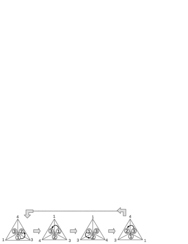
Figure 3: The permutating steps for plaquette quasiparticle ${S}_{\textbf{1}}$ to complete a circle around the center.

The three spins in one triangular plaquette are highly entangled with each other. The entropy of reduced density operator of the triple spin quasiparticle can be used as quantification of quantum entanglement. We compute the reduced density operator of $S^{+}\rangle_{B}$ for plaquette operator $S_{\textbf{2}}=\sigma^{y}_{2}\sigma^{x}_{3}\sigma^{z}_{4}$. The density operator is calculated by tracing out spin ”1”, i.e., $\rho_{{}_{S_{\textbf{2}}}}(S^{+}\rangle_{B})=Tr_{{}_{[1]}}\left[|S^{+}\rangle_{BB}\langle{S^{+}}|]_{[1234]}\right]$,

$$\rho_{{}_{S_{\textbf{2}}}}(|S^{+}\rangle_{B})=\left(\begin{array}[]{cccc}1&i&0&0\\ -i&-1&0&0\\ 0&0&1&-i\\ 0&0&-i&-1\\ \end{array}\right)\;.$$ (132)

The eigenvalue of this density operators is $\vec{\lambda}=[\sqrt{2},\sqrt{2},0,0].$ Only the two non-zero eigenvalues, $\lambda_{1}=\sqrt{2}$ and $\lambda_{2}=\sqrt{2}$, contribute to von Neumann entropy,

$$S(\rho)=-\lambda_{1}Log[\lambda_{1}]-\lambda_{2}Log[\lambda_{2}]=-\sqrt{2}Log[{{2}}].$$ (133)

the numerical value of von Neumann entropy $S(\rho)=-0.980258$. The quantum entanglement of the three spin in plaquette $S_{\textbf{2}}$ is not trivial. We can continue to calculate the reduced density operator and von Neumann entropy for other plaquette operators, $S_{\textbf{3}}=\sigma^{y}_{4}\sigma^{x}_{1}\sigma^{z}_{2}$ and $S_{\textbf{1}}$.

The reduced density operator of is originally based on the spatial order $[1423]$. If we modify the spatial ordering of the four spins in the eigenstate, the final density density operator are exactly the same as the original spatial ordering. Thus the fours are essentially not spatially indistinguishable.

IV Summary

Composite particle of multi-spin clusters in strongly correlated quantum many body system bear nontrivial statistics beyond boson and fermion. We extended the textbook definition for quantum statistics of two elementary particle to composite particle consist of many particles. The generalized definition is applied to study the quantum statistics of double-spin clusters and triple-spin quasiparticles in a triangular star quantum model. The eigenstates of this model are genuine entangled four qubit states. This Hamiltonian spontaneously generated eigenstates which shows some similar but different internal structure as Greenberger-Horne-Zeilinger state and Yeo-Chua’s genuine entangled states.

With the complete eigenenergy levels and explicit spin configuration of eigenstates, we found the zero energy state is an anti-symmetric state of two double-spin clusters, the highest excited state is a symmetric state of two double-spin clusters. In zero energy level and the highest energy level, two double-spin clusters behaves as boson. While in ground state and other intermediate excited state, the double-spin cluster shows fermionic behavior. This is partly because the ground state here is minimally frustrated states. If we choose different basis vector out of the four degenerated ground states, the statistical matrix produce the well known Pauli matrices. While Pauli matrix is convenient for constructing quantum logic gates.

We introduced frustrated coupling plaquette quasiparticles in this triangular star model. The triple-spin clusters states are the eigenstates of this model. Thus the excitation of triple-spin cluster is well defined quasiparticle. The Hamiltonian is mapped into a fermion pairing Hamiltonian of complex fermions. The statistical matrix of two triple-spin clusters on the first excited state is neither fermion nor boson. This suggest the plaquette quasiparticle obey exotic quantum statistics. The von Neumann entropy of the reduced density operator of the triangular plaquette excitation is also highly nontrivial. The plaquette quasiparticle in this triangular star model follows the same quantum symmetry as that in Kitaev honeycomb model, the main difference is here we introduced frustrations between quasiparticles and the quantum operator of these quasiparticle is only a half of the length as the hexagonal plaquette in Kitaev honeycomb model. Here the generalized definition of quantum statistics out of the textbook’s definition may help us to understand the non-abelian anyon in Kitaev honeycomb model.

V Acknowledgment

This work is supported by the Fundamental Research Funds for the Central Universities.

References

• (1) S. Y. Lee, J. Thompson, P. Kurzynski, A. Soeda, and D. Kaszlikowski, Phys. Rev. A 88, 063602 (2009), (2013).
• (2) C. Tichy, P. A. Bouvrie, and K. M${\o}$lmer, Phys. Rev. A 86, 042317 (2009), (2012).
• (3) C. Chudzicki, O. Oke, and W. K. Wootters, Phys. Rev. Lett. 104, 070402 (2010).
• (4) R. B. Laughlin, Phys. Rev. Lett. 50, 1395 (1983).
• (5) C. Nayak, S. H. Simon, A. Stern, M. Freedman and S. Das Sarma, Rev. Mod. Phys. 80, 1083 (2008).
• (6) A. Kitaev, Ann. Phys. 321, 2 (2006).
• (7) R. Horodecki, P. Horodecki, M. Horodecki, and K. Horodecki, Rev. Mod. Phys. 81, 865 (2009), and references therein, (2009).
• (8) M. V. d. Nest, Phys. Rev. Lett. 110, 060504 (2009), (2013).
• (9) C. J. Zhang, Y. X. Gong, Y. S. Zhang, and G. C. Guo, Phys. Rev. A 78, 042308 (2008).
• (10) F. Mintert and A. Buchleitner, Phys. Rev. Lett. 98, 140505 (2007).
• (11) J. W. Pan, Z. B. Chen, C. Y. Lu, H. Weinfurter, A. Zeilinger, M. Zukowski, Rev. Mod. Phys. 84, 777 (2012).
• (12) D. M. Greenberger, M.A. Horne, and A. Zeilinger, in Bell s Theorem, Quantum Theory, and Conceptions of the Universe, edited by M. Kafatos (Kluwer Academic, Dordrecht, 1989), pp. 69 C72, (1989).
• (13) A. Zeilinger, M.A. Horne, and D. M. Greenberger, in Proceedings of Squeezed States and Quantum Uncertainty, edited by D. Han, Y. S. Kim, and W.W. Zachary, NASA Conference Publication No. 3135 (NASA, Washington, DC, 1992), pp. 73 C81, (1992).
• (14) L. F. Zhao , B. H. Lai , F. Mei, Y. F. Yu, X. L. Feng and Z. M. Zhang, Chin. Phys. B 19, 094207 (2010).
• (15) Y. Yeo and W. K. Chua, Phys. Rev. Lett. 84, 4457 (2000).
• (16) V. Popkov, and M. Salerno, arXiv:1112.6352 [cond-mat.stat-mech], (2011).
• (17) M. Aulbach, Int. J. Quantum Inform. 10, 1230004 (2012).
• (18) P. Migda, J. Rodriguez-Laguna, and M. Lewenstein, arXiv:1305.1506v2 [quant-ph], ( 2013).
• (19) J. B. Park, E. Jung and D. Park, arXiv:1305.2012v1 [quant-ph], (2013).
• (20) S. H. Wang, Y. Lu, M. Gao, J. L. Cui, and J. L. Li, arXiv:1209.0063 [quant-ph], (2013).
• (21) Z. Z. Wang, and D. Markham, arXiv: 1210.1754 [quant-ph], (2012).
• (22) R. Moessner, S. L. Sondhi and P. Chandra, Phys. Rev. Lett. 84, 4457 (2000).
• (23) X. Y. Feng, G. M. Zhang, and T. Xiang, Phys. Rev. Lett. 98, 087204 (2007); H. D. Chen and J. P. Hu, Phys. Rev. B 76, 193101 (2007).
• (24) Y. Yu and T. Si, arXiv:0804.0483 (2008).
• (25) C. D. Batista, G. Ortiz, Phys. Rev. Lett. 86, 1082 (2001); M. S. Kochmanski, J. Tech. Phys., 36, 485 (1995), arXiv:cond-mat/9807388.
• (26) M. Y. Ye and X. M. Lin, Phys. Let. A 372, 4157 (2008).
• (27) W. K. Wootters, Phys. Rev. Lett. 80, 2245 (1998); S. Hill and W. K. Wootters , Phys. Rev. Lett. 78, 5022 (1997).