Variations on the magnetic torque acting on a wire

Abstract

The relation $\boldsymbol{M}=\boldsymbol{\mu}\times\boldsymbol{B}$ is presented in all elementary courses on electromagnetism but it is usually given just for the simple case of a rectangular wire. We will present a completely general but elementary proof of this relation together with two more advanced proof methods. We will then provide some extensions: non-closed wires and non-uniform magnetic field.

1 Introduction

The torque $\boldsymbol{M}$ acting on a wire induced by a uniform magnetic field $\boldsymbol{B}$ is given by the well known formula

$$\boldsymbol{M}=\boldsymbol{\mu}\times\boldsymbol{B}\ ,$$ (1)

where $\boldsymbol{\mu}$ is the magnetic dipole moment of the wire. In all elementary textbooks on electromagnetism (see e.g. Refs. [1, 2]) this formula is introduced by studying the example of a rectangular wire, for which the magnetic dipole moment can be explicitly written as $AI\boldsymbol{n}$, where $A$ is the area of the wire, $I$ is the current passing through it and $\boldsymbol{n}$ is the normal to the plane of the wire, with orientation consistent with that of the current.

Also in more advanced textbooks the complete derivation of Eq. (1) is usually skipped and just the example of the rectangular wires is presented. Two notable exceptions to this rule are the 8th volume of the Landau theoretical physics course (Ref. [3], pag. 128) and the book by J. D. Jackson (Ref. [4], pag. 188-190): the (sketch of the) proof by Landau relies on a variation on the theme of the Stokes theorem

$$\oint\mathrm{d}\boldsymbol{\ell}\times\boldsymbol{X}=\int\mathrm{d}\boldsymbol{\sigma}\times(\boldsymbol{\nabla}\times\boldsymbol{X})+\int(\mathrm{d}\boldsymbol{\sigma}\cdot\boldsymbol{\nabla})\boldsymbol{X}-\int\mathrm{d}\boldsymbol{\sigma}(\boldsymbol{\nabla}\cdot\boldsymbol{X})\ ,$$ (2)

where $\boldsymbol{X}$ is a generic vector field and the integrals in the left and right hand side of the equation are line and surface integrals respectively. Jackson’s proof uses instead the identity

$$\int(f\boldsymbol{Y}\cdot\boldsymbol{\nabla}g+g\boldsymbol{Y}\cdot\boldsymbol{\nabla}f+fg\boldsymbol{\nabla}\cdot\boldsymbol{Y})\mathrm{d}^{3}\boldsymbol{r}=0$$ (3)

where $f$ and $g$ are scalar functions of the position and $\boldsymbol{Y}$ is a vector field of compact support.

We will present a completely elementary proof of Eq. (1) together with the ones by Landau and Jackson, reviewed here with some more details than in the original references. We will then show how the computation can be extended to the more general cases of non closed wires and non-uniform magnetic field.

2 An elementary proof

The starting point is the Lorentz force acting on an element $\mathrm{d}\boldsymbol{\ell}$ of the wire, which in SI units is

$$\mathrm{d}\boldsymbol{F}=I\,\mathrm{d}\boldsymbol{\ell}\times\boldsymbol{B}\ ,$$ (4)

where $I$ is the current. The torque acting on the wire is then

$$\boldsymbol{M}=I\oint\boldsymbol{r}\times(\mathrm{d}\boldsymbol{\ell}\times\boldsymbol{B})\ .$$ (5)

Let us now suppose the wire to be parametrized by the function $\boldsymbol{s}(t)$, with $t\in[0,1]$ a real parameter. In this case $\mathrm{d}\boldsymbol{\ell}=\dot{\boldsymbol{s}}\mathrm{d}t$ (we denote by the dot the derivation with respect to $t$) and Eq. (5) can be rewritten in the form

$$\boldsymbol{M}=I\int_{0}^{1}\boldsymbol{s}\times(\dot{\boldsymbol{s}}\times\boldsymbol{B})\mathrm{d}t\ .$$ (6)

By using the vectorial identity

$$\boldsymbol{X}\times(\boldsymbol{Y}\times\boldsymbol{Z})=\boldsymbol{Y}(\boldsymbol{X}\cdot\boldsymbol{Z})-\boldsymbol{Z}(\boldsymbol{X}\cdot\boldsymbol{Y})$$ (7)

we can rewrite Eq. (6) in the form

$$\boldsymbol{M}=I\int_{0}^{1}\Big{\{}\dot{\boldsymbol{s}}(\boldsymbol{s}\cdot\boldsymbol{B})-\boldsymbol{B}(\dot{\boldsymbol{s}}\cdot\boldsymbol{s})\Big{\}}\,\mathrm{d}t$$ (8)

and it is simple to show that the second term vanishes in an uniform field: the vector $\boldsymbol{B}$ can be carried out of the integral, which finally reduces to

$$\int_{0}^{1}\dot{\boldsymbol{s}}\cdot\boldsymbol{s}\,\mathrm{d}t=\frac{1}{2}\int_{0}^{1}\frac{\mathrm{d}}{\mathrm{d}t}|\boldsymbol{s}|^{2}\,\mathrm{d}t=0$$ (9)

since $\boldsymbol{s}(0)=\boldsymbol{s}(1)$ for a closed wire.

By expressing the first term of Eq. (8) in components we have (summation on the repeated indices is always assumed when not otherwise stated)

$$\eqalign{&\int_{0}^{1}\Big{[}\dot{\boldsymbol{s}}(\boldsymbol{s}\cdot\boldsymbol{B})\Big{]}_{i}\,\mathrm{d}t=B_{j}\int_{0}^{1}\dot{s}_{i}s_{j}\,\mathrm{d}t=\\ &=\frac{1}{2}B_{j}\int_{0}^{1}(\dot{s}_{i}s_{j}+\dot{s}_{j}s_{i})\mathrm{d}t+\frac{1}{2}B_{j}\int_{0}^{1}(\dot{s}_{i}s_{j}-\dot{s}_{j}s_{i})\mathrm{d}t=\\ &=\frac{1}{2}B_{j}\int_{0}^{1}\frac{\mathrm{d}}{\mathrm{d}t}(s_{i}s_{j})\mathrm{d}t+\frac{1}{2}B_{j}\int_{0}^{1}(\dot{s}_{i}s_{j}-\dot{s}_{j}s_{i})\mathrm{d}t=\\ &=\frac{1}{2}\int_{0}^{1}\Big{[}\dot{\boldsymbol{s}}(\boldsymbol{B}\cdot\boldsymbol{s})-\boldsymbol{s}(\boldsymbol{B}\cdot\dot{\boldsymbol{s}})\Big{]}_{i}\mathrm{d}t}$$ (10)

where the total derivative term vanishes for the same reason as the integral in Eq. (9) does. On the other hand from the identity in Eq. (7) we have

$$(\boldsymbol{s}\times\dot{\boldsymbol{s}})\times\boldsymbol{B}=\dot{\boldsymbol{s}}(\boldsymbol{B}\cdot\boldsymbol{s})-\boldsymbol{s}(\boldsymbol{B}\cdot\dot{\boldsymbol{s}})\ ,$$ (11)

so that from Eq. (8), (9) and (10) we get

$$\boldsymbol{M}=\left(\frac{I}{2}\int_{0}^{1}(\boldsymbol{s}\times\dot{\boldsymbol{s}})\,\mathrm{d}t\right)\times\boldsymbol{B}\ ,$$ (12)

which is the desired Eq. (1) with the identification of the dipole magnetic moment

$$\boldsymbol{\mu}=\frac{I}{2}\int_{0}^{1}\boldsymbol{s}\times\dot{\boldsymbol{s}}\,\mathrm{d}t\ .$$ (13)

Going back to the line integral form we finally obtain

$$\boldsymbol{\mu}=\frac{I}{2}\oint\boldsymbol{r}\times\mathrm{d}\boldsymbol{\ell}\ ,$$ (14)

which for planar wires reduces to the simple expression $AI\boldsymbol{n}$, since the element of area is given by $\boldsymbol{n}\mathrm{d}A=\frac{1}{2}\boldsymbol{r}\times\mathrm{d}\boldsymbol{\ell}$.

3 Landau’s proof

In this section we will present a proof of Eq. (1) by using the identity Eq. (2), whose proof is given in A.

We first of all show how the form Eq. (14) of the magnetic dipole moment can be simplified by using the extension of the Stokes theorem proven in the appendix: by using Eq. (2) we immediately get (since $\boldsymbol{\nabla}\times\boldsymbol{r}=0$, $(\boldsymbol{a}\cdot\boldsymbol{\nabla})\boldsymbol{r}=\boldsymbol{a}$ and $\boldsymbol{\nabla}\cdot\boldsymbol{r}=3$)

$$\eqalign{\oint\mathrm{d}\boldsymbol{\ell}\times\boldsymbol{r}&=\int\mathrm{d}\boldsymbol{\sigma}\times(\boldsymbol{\nabla}\times\boldsymbol{r})+\int(\mathrm{d}\boldsymbol{\sigma}\cdot\boldsymbol{\nabla})\boldsymbol{r}-\int\mathrm{d}\boldsymbol{\sigma}(\boldsymbol{\nabla}\cdot\boldsymbol{r})=\\ &=\int\mathrm{d}\boldsymbol{\sigma}-3\int\mathrm{d}\boldsymbol{\sigma}=-2\int\mathrm{d}\boldsymbol{\sigma}}$$ (15)

and thus Eq. (14) becomes

$$\boldsymbol{\mu}=I\int\mathrm{d}\boldsymbol{\sigma}\ ,$$ (16)

which is the simplest extension to non planar wires of the expression $\boldsymbol{\mu}=AI\boldsymbol{n}$ valid in the planar case. Clearly the result of Eq. (16) does not depend on the choice of the surface of integration: if we denote by $\boldsymbol{c}$ a constant vector, the difference between the (projection on $\boldsymbol{c}$ of the) results obtained with two different choices $\Sigma_{1}$ and $\Sigma_{2}$ is given by

$$\boldsymbol{c}\cdot(\boldsymbol{\mu}_{1}-\boldsymbol{\mu}_{2})=I\left(\int_{\Sigma_{1}}\mathrm{d}\boldsymbol{\sigma}\cdot\boldsymbol{c}-\int_{\Sigma_{2}}\mathrm{d}\boldsymbol{\sigma}\cdot\boldsymbol{c}\right)=I\int_{V_{12}}(\boldsymbol{\nabla}\cdot\boldsymbol{c})\,\mathrm{d}^{3}\boldsymbol{r}=0\ ,$$ (17)

where $V_{12}$ is the volume bounded by the surfaces $\Sigma_{1}$ and $\Sigma_{2}$. Since this is true for every $\boldsymbol{c}$ we conclude that $\boldsymbol{\mu}_{1}=\boldsymbol{\mu}_{2}$.

In order to apply Eq. (2) to the computation of the torque it is convenient to use the following vectorial identity

$$\boldsymbol{X}\times(\boldsymbol{Y}\times\boldsymbol{Z})+\boldsymbol{Y}\times(\boldsymbol{Z}\times\boldsymbol{X})+\boldsymbol{Z}\times(\boldsymbol{X}\times\boldsymbol{Y})=0$$ (18)

and rewrite Eq. (5) in the form

$$\boldsymbol{M}=-I\oint\mathrm{d}\boldsymbol{\ell}\times(\boldsymbol{B}\times\boldsymbol{r})+I\oint(\boldsymbol{r}\times\mathrm{d}\boldsymbol{\ell})\times\boldsymbol{B}\ .$$ (19)

By comparison with Eq. (14) the second term can be recast in the form $2\boldsymbol{\mu}\times\boldsymbol{B}$, while applying Eq. (2) to the first term we get

$$\eqalign{&I\oint\mathrm{d}\boldsymbol{\ell}\times(\boldsymbol{B}\times\boldsymbol{r})=I\int\mathrm{d}\boldsymbol{\sigma}\times\Big{(}\boldsymbol{\nabla}\times(\boldsymbol{B}\times\boldsymbol{r})\Big{)}+\\ &+I\int(\mathrm{d}\boldsymbol{\sigma}\cdot\boldsymbol{\nabla})(\boldsymbol{B}\times\boldsymbol{r})-I\int\mathrm{d}\boldsymbol{\sigma}\Big{(}\boldsymbol{\nabla}\cdot(\boldsymbol{B}\times\boldsymbol{r})\Big{)}\ .}$$ (20)

By using the relations (which can be easily checked by direct computation)

$$\eqalign{&\boldsymbol{\nabla}\times(\boldsymbol{B}\times\boldsymbol{r})=2\boldsymbol{B}\\ &(\mathrm{d}\boldsymbol{\sigma}\cdot\boldsymbol{\nabla})(\boldsymbol{B}\times\boldsymbol{r})=\boldsymbol{B}\times\mathrm{d}\boldsymbol{\sigma}\\ &\boldsymbol{\nabla}\cdot(\boldsymbol{B}\times\boldsymbol{r})=0}$$ (21)

and Eq. (16) we thus get

$$I\oint\mathrm{d}\boldsymbol{\ell}\times(\boldsymbol{B}\times\boldsymbol{r})=2I\int\mathrm{d}\boldsymbol{\sigma}\times\boldsymbol{B}+I\int\boldsymbol{B}\times\mathrm{d}\boldsymbol{\sigma}=I\int\mathrm{d}\boldsymbol{\sigma}\times\boldsymbol{B}=\boldsymbol{\mu}\times\boldsymbol{B}\ .$$ (22)

Using this result in Eq. (19) we finally obtain Eq. (1).

4 Jackson’s proof

This proof makes use of Eq. (3), which is easily proven: since we assumed $\boldsymbol{Y}$ to be a function of compact support we have, by using the divergence theorem for a large enough volume $V$ (bounded by the surface $\Sigma$),

$$\int_{V}\boldsymbol{\nabla}\cdot(fg\boldsymbol{Y})\mathrm{d}^{3}\boldsymbol{r}=\int_{\Sigma}fg\,\mathrm{d}\boldsymbol{\sigma}\cdot{\boldsymbol{Y}}=0\ ,$$ (23)

since $\boldsymbol{Y}$ vanishes on $\Sigma$. By using the identity

$$\boldsymbol{\nabla}\cdot(fg\boldsymbol{Y})=f\boldsymbol{Y}\cdot\boldsymbol{\nabla}g+g\boldsymbol{Y}\cdot\boldsymbol{\nabla}f+fg\boldsymbol{\nabla}\cdot\boldsymbol{Y}$$ (24)

we thus get Eq. (3).

The starting point is Eq. (5), which can be rewritten by noting that the current density $\boldsymbol{j}$ has support on the wire and that $I\mathrm{d}\boldsymbol{\ell}=\boldsymbol{j}\mathrm{d}^{3}\boldsymbol{r}$, thus

$$\boldsymbol{M}=I\oint\boldsymbol{r}\times(\mathrm{d}\boldsymbol{\ell}\times\boldsymbol{B})=\int\boldsymbol{r}\times(\boldsymbol{j}\times\boldsymbol{B})\mathrm{d}^{3}\boldsymbol{r}\ .$$ (25)

By using Eq. (7) this expression becomes

$$\boldsymbol{M}=\int\boldsymbol{j}(\boldsymbol{r}\cdot\boldsymbol{B})\mathrm{d}^{3}\boldsymbol{r}-\int\boldsymbol{B}(\boldsymbol{r}\cdot\boldsymbol{j})\mathrm{d}^{3}\boldsymbol{r}\ .$$ (26)

If we now use Eq. (3) with $f=g=r_{i}$ (component $i$ of $\boldsymbol{r}$) and $\boldsymbol{Y}=\boldsymbol{j}$, remembering that $\boldsymbol{\nabla}\cdot\boldsymbol{j}=0$, we get (no summation over repeated indices)

$$0=\int(f\boldsymbol{Y}\cdot\boldsymbol{\nabla}g+g\boldsymbol{Y}\cdot\boldsymbol{\nabla}f)\mathrm{d}^{3}\boldsymbol{r}=2\int r_{i}j_{i}\,\mathrm{d}^{3}\boldsymbol{r}$$ (27)

and by summing over $i$ we obtain

$$\int\boldsymbol{r}\cdot\boldsymbol{j}\,\mathrm{d}^{3}\boldsymbol{r}=0\ ,$$ (28)

so the second term of Eq. (26) vanishes in an uniform magnetic field.

By using instead $f=r_{i}$, $g=r_{k}$ and $\boldsymbol{Y}=\boldsymbol{j}$ we get (again no summation on indices)

$$\int(r_{i}j_{k}+r_{k}j_{i})\mathrm{d}^{3}\boldsymbol{r}=0$$ (29)

and, by means of manipulations analogous to the ones in Eq. (10), we obtain

$$\int\boldsymbol{j}(\boldsymbol{r}\cdot\boldsymbol{B})\mathrm{d}^{3}\boldsymbol{r}=\frac{1}{2}\int\Big{(}\boldsymbol{j}(\boldsymbol{B}\cdot\boldsymbol{r})-\boldsymbol{r}(\boldsymbol{B}\cdot\boldsymbol{j})\Big{)}\mathrm{d}^{3}\boldsymbol{r}=\frac{1}{2}\int(\boldsymbol{r}\times\boldsymbol{j})\times\boldsymbol{B}\mathrm{d}^{3}\boldsymbol{r}\ ,$$ (30)

so that

$$\boldsymbol{M}=\frac{1}{2}\int(\boldsymbol{r}\times\boldsymbol{j})\times\boldsymbol{B}\mathrm{d}^{3}\boldsymbol{r}\ .$$ (31)

By using again the fact that $I\mathrm{d}\boldsymbol{\ell}=\boldsymbol{j}\mathrm{d}^{3}\boldsymbol{x}$ we see by comparison with Eq. (14) that

$$\boldsymbol{\mu}=\frac{1}{2}\int\boldsymbol{r}\times\boldsymbol{j}\mathrm{d}^{3}\boldsymbol{r}$$ (32)

and Eq. (31) thus reduces to Eq. (1).

5 Comments and extensions

We have seen in the previous sections that the torque generated by an uniform magnetic field $\boldsymbol{B}$ on a wire is given by

$$\boldsymbol{M}=\boldsymbol{\mu}\times\boldsymbol{B}\ ,$$ (33)

where the magnetic dipole moment $\boldsymbol{\mu}$ has the following equivalent definitions:

$$\boldsymbol{\mu}=\frac{I}{2}\int_{0}^{1}\boldsymbol{s}\times\dot{\boldsymbol{s}}\,\mathrm{d}t=\frac{I}{2}\oint\boldsymbol{r}\times\mathrm{d}\boldsymbol{\ell}=I\int\mathrm{d}\boldsymbol{\sigma}=\frac{1}{2}\int\boldsymbol{r}\times\boldsymbol{j}\mathrm{d}^{3}\boldsymbol{r}\ .$$ (34)

It is instructive to go through the different proofs presented of the relation Eq. (33) to search for the key ingredients used: from the first proof it is clear that, for a formula like Eq. (33) to be valid, the wire must be closed, an aspect whose importance is not completely evident in the usual example of the rectangular wire. This same requirement is naturally fundamental also for the second proof, since the Stokes theorem could not be applied to an open wire, and, although in a less trivial way, it is fundamental also in the third proof: there the main ingredient was current conservation, but the current would not be conserved in an open wire (see also below). Also, in all the proofs, the uniformity of the magnetic field was crucial to carry $\boldsymbol{B}$ out of the integration and factorize $\boldsymbol{\mu}$.

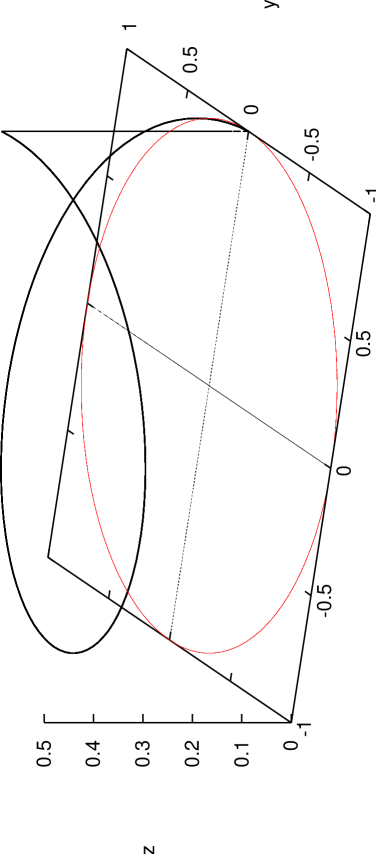
Figure 1: The wire parametrically represented by Eq. (35) with $\alpha=1$.

The first form of Eq. (34) is usually the most direct one to use in computations involving non-planar wires which are not trivially decomposable into planar ones. A simple non-trivial example is the wire in Fig. (1), whose parametrization is

$$\boldsymbol{s}(t)=\left\{\begin{array}[]{ll}\cos(4\pi t)\hat{x}+\sin(4\pi t)\hat{y}+\alpha t\hat{z}&t\in[0,1/2]\\ \rule{0.0pt}{14.22636pt}\hat{x}+\alpha(1-t)\hat{z}&t\in(1/2,1]\end{array}\right.\ .$$ (35)

It is simple to show that

$$\int_{0}^{1}\boldsymbol{s}\times\dot{\boldsymbol{s}}\,\mathrm{d}t=\alpha\hat{y}+2\pi\hat{z}$$ (36)

and thus the magnetic dipole moment of the wire parametrized by Eq. (35) is

$$\boldsymbol{\mu}=\frac{I\alpha}{2}\hat{y}+I\pi\hat{z}\ ,$$ (37)

which clearly reduce to the planar result $AI\hat{z}$, with $A=\pi$, when $\alpha=0$.

Various extensions of the result in Eq. (33)-(34) can easilly be performed: a particularly simple one is to consider a non-closed wire, i.e. $\boldsymbol{\Delta}=\boldsymbol{s}(1)-\boldsymbol{s}(0)\neq 0$. Clearly in this case on the wire it is acting also a net force: from Eq. (4) it is immediate to get for the total force the expression

$$\boldsymbol{F}=I\boldsymbol{\Delta}\times\boldsymbol{B}$$ (38)

and collecting the previously vanishing terms in Eq. (9)-(10) we obtain for the torque

$$\eqalign{\boldsymbol{M}&=\boldsymbol{\mu}\times\boldsymbol{B}+\frac{I}{2}\big{(}\boldsymbol{s}(1)(\boldsymbol{s}(1)\cdot\boldsymbol{B})-\boldsymbol{B}|\boldsymbol{s}(1)|^{2}\big{)}-\\ &\qquad-\frac{I}{2}\big{(}\boldsymbol{s}(0)(\boldsymbol{s}(0)\cdot\boldsymbol{B})-\boldsymbol{B}|\boldsymbol{s}(0)|^{2}\big{)}=\\ &=\boldsymbol{\mu}\times\boldsymbol{B}+\frac{I}{2}\boldsymbol{s}(1)\times(\boldsymbol{s}(1)\times\boldsymbol{B})-\\ &\qquad-\frac{I}{2}\boldsymbol{s}(0)\times(\boldsymbol{s}(0)\times\boldsymbol{B})\ ,}$$ (39)

where now $\boldsymbol{\mu}$ is defined by the first expression in Eq. (34). Since a net force is acting on the wire, the torque depends on the choice of the pole used (i.e. on the origin of the coordinates in our computation) and Eq. (39) can not in general be written in term of $\boldsymbol{\Delta}$ only; this happens only if we choose the pole in $\boldsymbol{s}(0)$, in which case Eq. (39) collapses to

$$\boldsymbol{M}=\boldsymbol{\mu}\times\boldsymbol{B}+\frac{I}{2}\boldsymbol{\Delta}\times(\boldsymbol{\Delta}\times\boldsymbol{B})\quad(\,\mathrm{pole\ in\ }\boldsymbol{s}(0)\,)\ .$$ (40)

This result can be obtained also using the methods of Sec. 4 by noting that, for a non-closed wire, the current is not conserved and a source and a sink have to be present at the wire endings:

$$\boldsymbol{\nabla}\cdot\boldsymbol{j}=I\delta(\boldsymbol{r}-\boldsymbol{s}(0))-I\delta(\boldsymbol{r}-\boldsymbol{s}(1))\ .$$ (41)

Another possible extension is the one to a non uniform magnetic field (again for a closed wire). Let us consider for simplicity only the first linear correction to the uniform field case:

$$\boldsymbol{B}(\boldsymbol{r})=\boldsymbol{b}+\underline{\boldsymbol{a}}\boldsymbol{r}\ ,$$ (42)

where $\boldsymbol{b}$ is a constant vector and $\underline{\boldsymbol{a}}$ is a linear operator, i.e. in component we have

$$B_{i}(\boldsymbol{r})=b_{i}+a_{ij}r_{j}\ .$$ (43)

The requirement $\boldsymbol{\nabla}\cdot\boldsymbol{B}=0$ imposes the restriction $\mathrm{Tr}\underline{\boldsymbol{a}}=0$ and, if we further assume that the currents that generate $\boldsymbol{B}$ are far away from the wire (“far away” means here that these currents do not contribute to the various line or surface integrals), from $\boldsymbol{\nabla}\times\boldsymbol{B}=0$ the relation $a_{ij}=a_{ji}$ follows, i.e. the matrix $\underline{\boldsymbol{a}}$ is symmetric. Since Eq. (8) is linear in $\boldsymbol{B}$, we can calculate the corrective term to $\boldsymbol{M}$ by simply using $\boldsymbol{b}=0$. We than have (using $\boldsymbol{s}(0)=\boldsymbol{s}(1)$)

$$\eqalign{&\int_{0}^{1}\Big{[}\boldsymbol{B}(\dot{\boldsymbol{s}}\cdot\boldsymbol{s})\Big{]}_{i}\mathrm{d}t=a_{ij}\int_{0}^{1}s_{j}\dot{s}_{k}s_{k}\mathrm{d}t=\\ &=\frac{1}{2}a_{ij}\int_{0}^{1}s_{j}\frac{\mathrm{d}}{\mathrm{d}t}(s_{k})^{2}\mathrm{d}t=-\frac{1}{2}\int_{0}^{1}(s_{k})^{2}a_{ij}\dot{s}_{j}\mathrm{d}t}$$ (44)

and thus

$$\int_{0}^{1}\boldsymbol{B}(\dot{\boldsymbol{s}}\cdot\boldsymbol{s})\mathrm{d}t=-\frac{1}{2}\oint r^{2}\underline{\boldsymbol{a}}\mathrm{d}\boldsymbol{\ell}\ .$$ (45)

On the other hand

$$\int_{0}^{1}\dot{\boldsymbol{s}}(\boldsymbol{s}\cdot\boldsymbol{B})\mathrm{d}t=\oint\mathrm{d}\boldsymbol{\ell}\big{(}\boldsymbol{r}\cdot(\underline{\boldsymbol{a}}\boldsymbol{r})\big{)}$$ (46)

and we thus obtain for the torque caused by the non-uniform magnetic field in Eq. (42) the expression

$$\boldsymbol{M}=\boldsymbol{\mu}\times\boldsymbol{b}+\frac{I}{2}\oint r^{2}\underline{\boldsymbol{a}}\mathrm{d}\boldsymbol{\ell}-I\oint\mathrm{d}\boldsymbol{\ell}\big{(}\boldsymbol{r}\cdot(\underline{\boldsymbol{a}}\boldsymbol{r})\big{)}\ .$$ (47)

The second term can be written also as a surface integral, indeed if we use the result Eq. (72) of B with $\boldsymbol{B}$ given by Eq. (42) we get

$$\boldsymbol{M}=\boldsymbol{\mu}\times\boldsymbol{b}+I\int\mathrm{d}\boldsymbol{\sigma}\times(\underline{\boldsymbol{a}}\boldsymbol{r})+I\int\boldsymbol{r}\times(\underline{\boldsymbol{a}}\mathrm{d}\boldsymbol{\sigma})$$ (48)

Clearly in the non-uniform field case also a non-vanishing net force is in general present, which, by using Eq. (2) (remembering that $\boldsymbol{\nabla}\cdot\boldsymbol{B}=0$ and $\boldsymbol{\nabla}\times\boldsymbol{B}=0$), can be written as

$$\boldsymbol{F}=\int(\mathrm{d}\boldsymbol{\sigma}\cdot\boldsymbol{\nabla})\boldsymbol{B}=\underline{\boldsymbol{a}}\boldsymbol{\mu}=\boldsymbol{\nabla}(\boldsymbol{\mu}\cdot\boldsymbol{B})$$ (49)

If we denote by $b$ the modulus of $\boldsymbol{b}$, by $a$ a typical value of $\underline{\boldsymbol{a}}$ and we consider a wire of typical linear dimension $L$, the contributions in Eq. (47)-(49) are of order

$$M\sim bL^{2}+aL^{3}\qquad F\sim aL^{2}$$ (50)

and the first of these equations can conveniently be rewritten as

$$M\sim bL^{2}\left(1+\frac{L}{\lambda}\right)\ ,$$ (51)

where $\lambda=b/a$ is the typical length scale of variation of the magnetic field in Eq. (42). It is then clear that, as intuitively obvious, the non uniformity of the magnetic field can be neglected as far as $L\ll\lambda$. For dimensional reasons the force in Eq. (50) has one power of $L$ missing with respect to the torque, but dimensionality would suggests also the presence of a term $bL$, which is absent since in an uniform field no net force is acting on the wire. Because of the absence of this leading contribution, the non uniformity of the magnetic field can not be neglected even for small wires in the force computation.

For a generic non-uniform magnetic field, Eq. (42) is just the first term of a Taylor expansion, whose general form is

$$B_{i}=a^{(0)}_{i}+a^{(1)}_{ij_{1}}r_{j_{1}}+a^{(2)}_{ij_{1}j_{2}}r_{j_{1}}r_{j_{2}}+\cdots+a^{(n)}_{ij_{1}\cdots j_{n}}r_{j_{1}}\cdots r_{j_{n}}+\cdots$$ (52)

where $a^{(n)}_{ij_{1}\cdots j_{n}}$ is symmetric under permutations of $j_{1},\ldots,j_{n}$. The condition $\boldsymbol{\nabla}\cdot\boldsymbol{B}=0$ becomes for the $n-$th term

$$0=\partial_{i}B_{i}=a^{(n)}_{ij_{i}\cdots j_{n}}\partial_{i}(r_{j_{1}}\cdots r_{j_{n}})=na^{(n)}_{iij_{2}\cdots j_{n}}r_{j_{2}}\cdots r_{j_{n}}$$ (53)

and the condition $\boldsymbol{\nabla}\times\boldsymbol{B}=0$ gives

$$0=\partial_{\alpha}B_{\beta}-\partial_{\beta}B_{\alpha}=n(a^{(n)}_{\beta\alpha j_{2}\cdots j_{n}}-a^{(n)}_{\alpha\beta j_{2}\cdots j_{n}})r_{j_{2}}\cdots r_{j_{n}}\ ,$$ (54)

so that $a^{(n)}_{ij_{1}\cdots j_{n}}$ is again completely symmetric and traceless. It is then not difficult to generalize Eq. (47) and Eq. (48). We can introduce a characteristic length $\lambda_{(n)}$ for every term in Eq. (52) by

$$\lambda_{(n)}=\sqrt[n]{\frac{a^{(0)}}{a^{(n)}}}\ ,$$ (55)

where $a^{(0)}$ and $a^{(n)}$ stand here for typical values, and Eq. (51) generalizes to

$$M\sim a^{(0)}L^{2}\Big{[}1+\frac{L}{\lambda_{(1)}}+\left(\frac{L}{\lambda_{(2)}}\right)^{2}+\cdots+\left(\frac{L}{\lambda_{(n)}}\right)^{n}+\cdots\Big{]}\ .$$ (56)

For a typical magnetic field we have

$$\lambda_{(1)}\lesssim\lambda_{(2)}\lesssim\cdots\lesssim\lambda_{(n)}\lesssim\cdots$$ (57)

and we thus see that the expansion Eq. (56) can be truncated to the $n-$th term if the typical linear dimension of the wire satisfies

$$\frac{L}{\lambda_{(n+1)}}\left(\frac{\lambda_{(n)}}{\lambda_{(n+1)}}\right)^{n}\ll 1\ .$$ (58)

6 Conclusions

We discussed three different methods to compute the torque acting on a generic wire in an uniform magnetic field, the first is completely elementary, the other two present a higher degree of mathematical sophistication. We have then shown how the computation can be generalized to the cases of non-closed wires and non-uniform magnetic field.

Appendix A An extension of the Stokes theorem

The Stokes theorem relates the circuitation of a field along a closed curve to the flux of its curl: in formulae (see e.g. Ref. [5])

$$\oint\mathrm{d}\boldsymbol{\ell}\cdot\boldsymbol{X}=\int\mathrm{d}\boldsymbol{\sigma}\cdot(\boldsymbol{\nabla}\times\boldsymbol{X})\ ,$$ (59)

while we are interested in line integrals of the form

$$\boldsymbol{I}=\oint\mathrm{d}\boldsymbol{\ell}\times\boldsymbol{X}\ .$$ (60)

In order to make use of the Stokes theorem in the computation of the r.h.s of Eq. (60), it is convenient to take the scalar product of $\boldsymbol{I}$ with a constant vector, which we will denote by $\boldsymbol{c}$:

$$\boldsymbol{c}\cdot\boldsymbol{I}=\oint\boldsymbol{c}\cdot(\mathrm{d}\boldsymbol{\ell}\times\boldsymbol{X})=\oint\mathrm{d}\boldsymbol{\ell}\cdot(\boldsymbol{X}\times\boldsymbol{c})=\int\mathrm{d}\boldsymbol{\sigma}\cdot\Big{[}\boldsymbol{\nabla}\times(\boldsymbol{X}\times\boldsymbol{c})\Big{]}\ ,$$ (61)

where in the intermediate step we used the identity $\boldsymbol{A}\cdot(\boldsymbol{B}\times\boldsymbol{C})=\boldsymbol{B}\cdot(\boldsymbol{C}\times\boldsymbol{A})$ and the last identity is just the usual Stokes theorem.

Passing in components and remembering that $\boldsymbol{c}$ is a constant vector, we get

$$\eqalign{\Big{[}\boldsymbol{\nabla}\times(\boldsymbol{X}\times\boldsymbol{c})\Big{]}_{i}&=\epsilon_{ijk}\partial_{j}\epsilon_{klm}X_{l}c_{m}=\\ &=-\epsilon_{kji}\epsilon_{klm}\partial_{j}X_{l}c_{m}=\\ &=-(\delta_{jl}\delta_{im}-\delta_{jm}\delta_{il})\partial_{j}X_{l}c_{m}}$$ (62)

and thus

$$\boldsymbol{\nabla}\times(\boldsymbol{X}\times\boldsymbol{c})=-\boldsymbol{c}(\boldsymbol{\nabla}\cdot\boldsymbol{X})+(\boldsymbol{c}\cdot\boldsymbol{\nabla})\boldsymbol{X}\ .$$ (63)

In a similar way it can be shown that

$$\boldsymbol{c}\times(\boldsymbol{\nabla}\times\boldsymbol{X})=-(\boldsymbol{c}\cdot\boldsymbol{\nabla})\boldsymbol{X}+\boldsymbol{\nabla}(\boldsymbol{c}\cdot\boldsymbol{X})$$ (64)

and by summing theese two equations we get

$$\boldsymbol{\nabla}\times(\boldsymbol{X}\times\boldsymbol{c})=(\boldsymbol{\nabla}\times\boldsymbol{X})\times\boldsymbol{c}+\boldsymbol{\nabla}(\boldsymbol{c}\cdot\boldsymbol{X})-\boldsymbol{c}(\boldsymbol{\nabla}\cdot\boldsymbol{X})\ .$$ (65)

By using this identity in Eq. (61) we obtain

$$\eqalign{\boldsymbol{c}\cdot\boldsymbol{I}&=\int\mathrm{d}\boldsymbol{\sigma}\cdot\Big{\{}(\boldsymbol{\nabla}\times\boldsymbol{X})\times\boldsymbol{c}\Big{\}}+\int\mathrm{d}\boldsymbol{\sigma}\cdot\boldsymbol{\nabla}(\boldsymbol{c}\cdot\boldsymbol{X})-\\ &\qquad-\int\boldsymbol{c}\cdot\mathrm{d}\boldsymbol{\sigma}(\boldsymbol{\nabla}\cdot\boldsymbol{X})=\\ &=\int\boldsymbol{c}\cdot\Big{\{}\mathrm{d}\boldsymbol{\sigma}\times(\boldsymbol{\nabla}\times\boldsymbol{X})\Big{\}}+\int\mathrm{d}\boldsymbol{\sigma}\cdot\boldsymbol{\nabla}(\boldsymbol{c}\cdot\boldsymbol{X})-\\ &\qquad-\int\boldsymbol{c}\cdot\mathrm{d}\boldsymbol{\sigma}(\boldsymbol{\nabla}\cdot\boldsymbol{X})}$$ (66)

and by replacing the constant vector $\boldsymbol{c}$ by the versors of the coordinate axes we finally get the desired extension of the Stokes theorem

$$\boldsymbol{I}=\int\mathrm{d}\boldsymbol{\sigma}\times(\boldsymbol{\nabla}\times\boldsymbol{X})+\int(\mathrm{d}\boldsymbol{\sigma}\cdot\boldsymbol{\nabla})\boldsymbol{X}-\int\mathrm{d}\boldsymbol{\sigma}(\boldsymbol{\nabla}\cdot\boldsymbol{X})\ .$$ (67)

Appendix B Another variant of the Stokes theorem

In this appendix we will deduce another variant of the Stokes theorem, this time referred to integrals of the form of the torque:

$$\boldsymbol{J}=\oint\boldsymbol{r}\times(\mathrm{d}\boldsymbol{\ell}\times\boldsymbol{B})$$ (68)

Multiplying $\boldsymbol{J}$ by the constant vector $\boldsymbol{c}$ we can use

$$\boldsymbol{c}\cdot\Big{(}\boldsymbol{r}\times(\mathrm{d}\boldsymbol{\ell}\times\boldsymbol{B})\Big{)}=(\mathrm{d}\boldsymbol{\ell}\times\boldsymbol{B})\cdot(\boldsymbol{c}\times\boldsymbol{r})=\mathrm{d}\boldsymbol{\ell}\cdot\Big{(}\boldsymbol{B}\times(\boldsymbol{c}\times\boldsymbol{r})\Big{)}$$ (69)

to get, by the Stokes theorem,

$$\boldsymbol{c}\cdot\boldsymbol{J}=\int\mathrm{d}\boldsymbol{\sigma}\cdot\Big{\{}\boldsymbol{\nabla}\times\Big{(}\boldsymbol{B}\times(\boldsymbol{c}\times\boldsymbol{r})\Big{)}\Big{\}}\ .$$ (70)

By proceeding as in Eq. (62) it can be shown that

$$\boldsymbol{\nabla}\times(\boldsymbol{Y}\times\boldsymbol{Z})=(\boldsymbol{Z}\cdot\boldsymbol{\nabla})\boldsymbol{Y}-(\boldsymbol{Y}\cdot\boldsymbol{\nabla})\boldsymbol{Z}+\boldsymbol{Y}(\boldsymbol{\nabla}\cdot\boldsymbol{Z})-\boldsymbol{Z}(\boldsymbol{\nabla}\cdot\boldsymbol{Y})$$ (71)

and, by using $\boldsymbol{\nabla}\cdot\boldsymbol{B}=0$ and $\boldsymbol{\nabla}\cdot(\boldsymbol{c}\times\boldsymbol{r})=0$, we get

$$\boldsymbol{c}\cdot\boldsymbol{J}=\int\mathrm{d}\boldsymbol{\sigma}\cdot\Big{[}\Big{(}(\boldsymbol{c}\times\boldsymbol{r})\cdot\boldsymbol{\nabla}\Big{)}\boldsymbol{B}\Big{]}+\boldsymbol{c}\cdot\int\mathrm{d}\boldsymbol{\sigma}\times\boldsymbol{B}\ .$$ (72)

For an uniform magnetic field only the last term survives and gives once again Eq. (1).

References

References

• [1] D.ย J.ย Griffiths, Introduction to Electrodynamics, 2nd ed. (Prentice Hall, Englewood Cliffs, New Jersey, 1989).
• [2] R.ย P.ย Feynman, R.ย B.ย Leighton, M.ย Sand, The Feynman Lectures on Physics, Mainly Electromagnetism and Matter (Addison-Wesley, Reading, Massachussetts, 1964).
• [3] L.ย D.ย Landau, E.ย M.ย Lifshitz and L.ย P.ย Pitaevskii, Electrodynamics of Continuous Media, 2nd ed. (Butterworth-Heinemann, Oxford, UK, 2004).
• [4] J.ย D.ย Jackson Classical Electrodynamics, 3rd ed. (John Wiley & Sons, Hoboken, New Jersey, 1999).
• [5] W.ย Rudin Principles of Mathematical Analysis, 3rd ed. (McGraw-Hill, New York, 1976).
• [6] J.ย Franklin Classical Electromagnetism (Pearson, San Francisco, CA, 2005)