Non-negative least squares for high-dimensional linear models: consistency and sparse recovery without regularization
Abstract
Least squares fitting is in general not useful for high-dimensional linear models, in which the number of predictors is of the same or even larger order of magnitude than the number of samples. Theory developed in recent years has coined a paradigm according to which sparsity-promoting regularization is regarded as a necessity in such setting. Deviating from this paradigm, we show that non-negativity constraints on the regression coefficients may be similarly effective as explicit regularization if the design matrix has additional properties, which are met in several applications of non-negative least squares (NNLS). We show that for these designs, the performance of NNLS with regard to prediction and estimation is comparable to that of the lasso. We argue further that in specific cases, NNLS may have a better -rate in estimation and hence also advantages with respect to support recovery when combined with thresholding. From a practical point of view, NNLS does not depend on a regularization parameter and is hence easier to use.
keywords:
[class=AMS]keywords:
and
t1Supported by the Cluster of Excellence ’Multimodal Computing and Interaction’ (MMCI) of Deutsche Forschungsgemeinschaft (DFG)
1 Introduction
Consider the linear regression model
| (1.1) |
where is a vector of observations, a design matrix, a vector of noise and a vector of coefficients to be estimated. Throughout this paper, we are concerned with a high-dimensional setting in which the number of unknowns is at least of the same order of magnitude as the number of observations , i.e. or even , in which case one cannot hope to recover the target if it does not satisfy one of various kinds of sparsity constraints, the simplest being that is supported on , . In this paper, we additionally assume that is non-negative, i.e. . This constraint is particularly relevant when modelling non-negative data, which emerge e.g. in the form of pixel intensity values of an image, time measurements, histograms or count data, economical quantities such as prices, incomes and growth rates. Non-negativity constraints occur naturally in numerous deconvolution and unmixing problems in diverse fields such as acoustics [31], astronomical imaging [2], hyperspectral imaging [1], genomics [30], proteomics [42], spectroscopy [19] and network tomography [34]; see [14] for a survey. As reported in these references, non-negative least squares (NNLS) yields at least reasonably good, sometimes even excellent results in practice, which may seem surprising in view of the simplicity of that approach. The NNLS problem is given by the quadratic program
| (1.2) |
which is a convex optimization problem that can be solved efficiently [27]. A minimizer of (1.2) will be referred to as an NNLS estimator. Solid theoretical support for the empirical success of NNLS from a statistical perspective scarcely appears in the literature. An early reference is [19] dating back already two decades. The authors show that, depending on and the sparsity of , NNLS may have a ’super-resolution’-property that permits reliable estimation of . Rather recently, sparse recovery of non-negative signals in a noiseless setting () has been studied in [7, 18, 54, 55]. One important finding of this body of work is that non-negativity constraints alone may suffice for sparse recovery, without the need to employ sparsity-promoting -regularization as usually. On the other hand, it remains unclear whether similar results continue to hold in a more realistic noisy setup. At first glance, the following considerations suggest a negative answer. The fact that NNLS, apart from sign constraints, only consists of a fitting term, fosters the intuition that NNLS is prone to overfitting, specifically in a high-dimensional setting. Usefulness of NNLS in such setting appears to be in conflict with the well-established paradigm that a regularizer is necessary to prevent over-adaptation to noise and to enforce desired structural properties of the solution, like sparsity of the vector of coefficients. As one of the main contributions of the present paper, we characterize the self-regularizing property which NNLS exhibits for a certain class of designs that turn out to be tailored to the non-negativity constraint, thereby disentangling the apparent conflict above and improving the understanding of the empirical success of NNLS. More precisely, we show that for these designs, NNLS is rather closely related to the non-negative lasso problem
| (1.3) |
the sign-constrained counterpart to the popular lasso problem [46], which is given by
| (1.4) |
where is a tuning parameter. Elaborating on the relation between NNLS and the non-negative lasso, we establish that for the aforementioned class of designs, NNLS achieves comparable performance with regard to prediction, estimation of and support recovery when combined with subsequent thresholding. We here refer to the monograph [8], the survey [51] and the retrospective [47] for an overview on the appealing performance guarantees established for the lasso in the last decade, which have, along with favourable computational properties, contributed to its enormous popularity in data analysis. In this paper, we argue that, in view of both theoretical considerations and empirical evidence, improvements of NNLS over the (non-negative) lasso are possible, even though they are limited to a comparatively small set of designs. Differences in performance arise from the bias of the -regularizer in (1.3) and (1.4) that is responsible for a in general sub-optimal rate for estimation of in the -norm [59]. Unlike for NNLS, a tuning parameter needs to be specified for the (non-negative) lasso, as it is necessary for all regularization based-methods. Selection of the tuning parameter by means of cross-validation increases the computational burden and may be error-prone if done by a grid search, since the grid could have an unfavourable range or a too small number of grid points. Theoretical results on how to set the regularization parameter are often available, but require a sufficient degree of acquaintance with existing literature and possibly also knowledge of quantities such as the noise level. The last issue has been withstanding problem of the lasso until recently. In [4] and [45] two related variants of the lasso are proposed that have similar theoretical guarantees, while the tuning parameter can be set without knowledge of the noise level. On the other hand, NNLS is directly applicable, since it is free of tuning parameters.
Outline and contributions of the paper. The paper significantly extends a previous conference publication [43], which contains the first systematic analysis of NNLS in a high-dimensional setting. Recently, Meinshausen [34] has independently studied the performance of NNLS in such a setting. His work is related to ours in Section 3. The paper is organized as follows. In Section 2 we work out the self-regularizing property NNLS may have in conjunction with certain design matrices. Equipped with that property, a bound on the prediction error is stated that resembles a corresponding ’slow rate’ bound available for the lasso. Developing further the connection to the lasso, we use techniques pioneered in Bickel et al. [5] to prove bounds on the estimation error in -norm, , and an improved bound on the prediction error of NNLS in Section 3. In Section 4, we finally provide bounds on the sup-norm error of NNLS. Hard thresholding of is proposed for sparse recovery, and a data-driven procedure for selecting the threshold is devised. Section 4 also contains a discussion of advantages and disadvantages of NNLS relative to the non-negative lasso. In Section 5, we have a closer look at several designs, which satisfy the conditions required throughout the paper. In Section 6, we discuss the empirical performance of NNLS in deconvolution and sparse recovery in comparison to standard methods, in particular to the non-negative lasso. The appendix contains most of the proofs, apart from those that have been placed into a supplement.
Notation.
We denote the usual -norm by
. The cardinality of a set is denoted by . Let be index
sets. For a matrix , denotes the matrix one obtains
by extracting the columns corresponding to . For ,
denotes the -th column of . The
matrix is the sub-matrix of by extracting rows in and columns
in . Likewise, for , is the
sub-vector corresponding to . Identity matrices and vectors of ones of
varying dimensions are denoted by respectively . The symbols and denote
componentwise inequalities and componentwise strict inequalities,
respectively. In addition, for some matrix , means that all
entries of are at least equal to a scalar . The
non-negative orthant is denoted by
. The standard simplex in , that is the set is denoted by . Lower and uppercase c’s like and etc. denote positive constants not depending on the
sample size whose values may differ from line to line. In general, the
positive integers and depend on . Landau’s symbols
are denoted by . Asymptotics is to be understood w.r.t.
a triangular array of observations .
Normalization. If not stated otherwise, the design matrix is considered as
deterministic, having its columns normalized such that ,
.
General linear position.
We say that the columns of are in general linear position in if the following condition (GLP) holds
| (1.5) |
where for , denotes the submatrix of consisting of the columns corresponding to .
2 Prediction error: a bound for ’self-regularizing’ designs
The main result of the following section is a bound on the excess error of NNLS that resembles the so-called slow rate bound of the lasso [24, 3, 8]. In contrast to the latter, the corresponding bound for NNLS only holds for a certain class of designs. We first show that extra conditions on the design are in fact necessary to obtain such bound. We then introduce a condition on that we refer to as ’self-regularizing property’ which is sufficient to establish a slow rate bound for NNLS. The term ’self-regularization’ is motivated from a resulting decomposition of the least squares objective into a modified fitting term and a quadratic term that plays a role similar to an -penalty on the coefficients. This finding provides an intuitive explanation for the fact that NNLS may achieve similar performance than the lasso, albeit no explicit regularization is employed.
2.1 A minimum requirement on the design for non-negativity being an actual constraint
In general, the non-negativity constraints in (1.2) may not be meaningful at all, given the fact that any least squares problem can be reformulated as a non-negative least squares problem with an augmented design matrix . More generally, NNLS can be as ill-posed as least squares if the following condition does not hold.
| (2.1) |
Condition requires the columns of be contained in the interior of a half-space containing the origin. If fails to hold, , so that there are infinitely many minimizers of the NNLS problem (1.2). If additionally and the columns of are in general linear position (condition in (1.5)), must be in the interior of . It then follows that , where denotes the polyhedral cone generated by the columns of . Consequently, the non-negativity constraints become vacuous and NNLS yields perfect fit for any observation vector . In light of this, constitutes a necessary condition for a possible improvement of NNLS over ordinary least squares.
2.2 Overfitting of NNLS for orthonormal design
Since NNLS is a pure fitting approach, over-adaptation to noise is a natural concern. Resistance to overfitting can be quantified in terms of when in (1.1). It turns out that condition is not sufficient to ensure that with high probability, as can be seen from studying orthonormal design, i.e. . Let be a standard Gaussian random vector. The NNLS estimator has the closed form expression
so that the distribution of each component of is given by a mixture of a point mass at zero and a half-normal distribution. We conclude that is of the order with high probability. The fact that is orthonormal is much stronger than the obviously necessary half-space constraint . In fact, as rendered more precisely in Section 5, orthonormal design turns out to be at the edge of the set of designs still leading to overfitting.
2.3 A sufficient condition on the design preventing NNLS from overfitting
We now present a sufficient condition has to satisfy so that overfitting is prevented. That condition arises as a direct strengthening of (). In order to quantify the separation required in , we define
| (2.2) |
Note that if and only if is fulfilled. Also note that with , it holds that . Introducing the Gram matrix , we have by convex duality that
| (2.3) |
i.e. in geometrical terms, equals the distance of the convex hull of the columns of (scaled by ) to the origin. Using terminology from support vector machine classification (e.g. [41], Sec. 7.2), can be interpreted as margin of a maximum margin hyperplane with normal vector separating the columns of from the origin. As argued below, in case that scales as a constant, overfitting is curbed. This is e.g. not fulfilled for orthonormal design, where (cf. Section 5).
Condition 1.
A design is said to have a self-regularizing property if there exists a constant so that with as defined in (2.2), it holds that .
The term ’self-regularization’ expresses the fact that the design itself automatically generates a regularizing term, as emphasized in the next proposition and the comments that follow. We point out that Proposition 1 is a qualitative statement preliminary to the main result of the section (Theorem 1) and mainly serves an illustrative purpose.
Proposition 1.
Consider the linear model (1.1) with and having entries that are independent random variables with zero mean and finite variance. Suppose that satisfies Condition 1. We then have
| (2.4) |
with , where is a projection onto an -dimensional subspace of and is a diagonal matrix, the diagonal entries being contained in . Moreover, if , then any minimizer of (2.4) obeys .
In Proposition 1, the pure noise fitting problem is decomposed into a fitting term with modified design matrix , a second term that can be interpreted as squared non-negative lasso penalty (cf. (1.3)) and an additional stochastic term of lower order. As made precise in the proof, the lower bound on implies that the -norm of any minimizer is upper bounded by a constant. Prevention of overfitting is then an immediate consequence under the further assumption that the term tends to zero. This holds under rather mild additional conditions on [33] or more stringent conditions on the tails of the noise distribution. As a last comment, let us make the connection of the r.h.s. of (2.4) to a non-negative lasso problem more explicit. Due to the correspondence of the level sets of the mappings and on , we have
| (2.5) |
where is a non-negative, monotonically increasing function of . Proposition 1 in conjunction with (2.5) provides a high-level understanding of what will be shown in the sequel, namely that NNLS may inherit desirable properties of the (non-negative) lasso with regard to prediction, estimation and sparsity of the solution.
2.4 Slow rate bound
Condition 1 gives rise to the following general bound on the -prediction error of NNLS. Note that in Theorem 1 below, it is not assumed that the linear model is specified correctly. Instead, we only assume that there is a fixed target to be approximated by a non-negative combination of the columns of .
Theorem 1.
Let , where is fixed and has i.i.d. zero-mean sub-Gaussian entries with parameter 111See Appendix A for background on sub-Gaussian random variables. Define
Suppose that satisfies Condition 1. Then, for any minimizer of the NNLS problem (1.2) and any , it holds with probability no less than that
| (2.6) |
for all .
Comparison with the slow rate bound of the lasso.
Theorem 1 bounds the excess error by a term of order , which implies that NNLS can be consistent in a regime in which the number of predictors is nearly exponential in the number of observations . That is, NNLS constitutes a ’persistent procedure’ in the spirit of Greenshtein and Ritov [24] who coined the notion of ’persistence’ as distinguished from classical consistency with a fixed number of predictors. The excess error bound of Theorem 1 is of the same order of magnitude as the corresponding bound of the lasso [24, 3, 8] that is typically referred to as slow rate bound. Since the bound (2.6) depends on , it is recommended to solve the quadratic program in (2.3) before applying NNLS, which is roughly of the same computational cost. Unlike Theorem 1, the slow rate bound of the lasso does not require any conditions on the design and is more favourable than (2.6) regarding the constants. In [52, 25], improvements of the slow rate bound are derived. On the other hand, the results for the lasso require the regularization parameter to be chosen appropriately.
Remark 1.
NNLS has been introduced as a tool for ’non-negative data’. In this context, the assumption of zero-mean noise in Theorem 1 is questionable. In case that the entries of have a positive mean, one can decompose into a constant term, which can be absorbed into the linear model, and a second term which has mean zero, so that Theorem 1 continues to be applicable.
3 Fast rate bound for prediction and bounds on the -error for estimation,
Within this section, we further elaborate on the similarity in performance of -regularization and NNLS for designs with a self-regularizing property. We show that the latter admits a reduction to the scheme pioneered in [5] to establish near-optimal performance guarantees of the lasso and the related Dantzig selector [13] with respect to estimation of and and prediction under a sparsity scenario. Similar results are shown e.g. in [10, 13, 50, 57, 36, 12, 59], and we shall state results of that flavour for NNLS below. Throughout the rest of the paper, the data-generating model (1.1) is considered for a sparse target with support .
Reduction to the scheme used for the lasso.
As stated in the next lemma, if the design satisfies Condition 1, the NNLS estimator has, with high probability, the property that has small -norm, or that is contained in the convex cone
| (3.1) |
The latter property is shared by the lasso and Dantzig selector with different values of the constant [13, 5].
Lemma 1.
Assume that , where has support , has i.i.d. zero-mean sub-Gaussian entries with parameter . Further assume that satisfies Condition 1. Denote . Then, for any , at least one of the following two events occurs with probability no less than :
The rightmost event is most favourable, since it immediately yields the assertion of Theorem 2 below. On the other hand, under the leftmost event, one is in position to carry over techniques used for analyzing the lasso. When combined with the following Condition 2, near-optimal rates with regard to estimation and prediction can be obtained.
Condition 2.
Let and for and ,
We say that the design satisfies the -restricted eigenvalue condition if there exists a constant so that
| (3.2) |
Condition 2 is introduced in [5]. It is weaker than several
other conditions such as those in [13, 36]
employed in the same context; for a comprehensive comparison of these and
related conditions, we refer to [50]. Moreover, we note that
Condition 2 is satisfied with overwhelming probability if
belongs to a rather broad class of random sub-Gaussian matrices with
independent rows as long as scales as [39].
Using Lemma 1, the next statement follows along the lines of the analysis in [5].
Theorem 2.
In addition to the conditions of Lemma 1, assume further that satisfies the -restricted eigenvalue condition. It then holds for any and any that
with probability no less than .
Theorem 2 parallels Theorem 7.2 in [5],
establishing that the lasso adapts to the underlying sparsity, since its
performance attains (apart from factors logarithmic in ) what could be achieved if the support were
known in advance. The rates of Theorem 2 for NNLS are the same
as those for the lasso, modulo (less favourable) multiplicative constants.
The required condition on the design is a combination of the self-regularizing
property and the restricted eigenvalue condition. At first glance, these two
conditions might appear to be contradicting each other, since the first one is
not satisfied if the off-diagonal entries of are too small, while
for , we have . We resolve this apparent contradiction in Section 5 by
providing designs satisfying both conditions simultaneously. The use
of Condition 2 in place of more restrictive conditions like
restricted isometry properties (RIP, [13]) used earlier
in the literature turns out to be crucial here, since these conditions
impose much stronger constraints on the magnitude of the off-diagonals entries of
as discussed in detail in [37].
A result of the same spirit as Theorem 2 is shown in the recent paper
[34] by Meinshausen who has independently studied the
performance of NNLS for high-dimensional linear models. That paper provides
an -bound for estimation of and a fast rate bound for
prediction with better constants than those in above theorem, even though the
required conditions are partly more restrictive. The ingredients leading to
those bounds are the self-regularizing property, which is termed ’positive
eigenvalue condition’ there, and the ’compatibility condition’ [50, 51]
which is used in place of Condition 2. We prefer the latter here,
because the ’compatibility condition’ is not sufficient to establish -bounds for
estimation for . As distinguished from our Theorem 2, a lower bound
on the minimum non-zero coefficient of is additionally required
in the corresponding result in [34].
4 Estimation error with respect to the norm and support recovery by thresholding
In the present section, we directly derive bounds on the -estimation error of NNLS without resorting to techniques and assumptions used in the analysis of the lasso. Instead, we build on the geometry underlying the analysis of NNLS for sparse recovery in the noiseless case [16, 17, 54, 18]. In light of the stated bounds, we subsequently study the performance of a thresholded NNLS estimator with regard to support recovery.
4.1 Main components of the analysis
In the sequel, we provide the main steps towards the results stated in this section. Basic to our approach is a decomposition of the NNLS problem into two sub-problems corresponding to the support and the off-support . For this purpose, we need to introduce the following quantities. For a given support , let and denote the projections on the subspace spanned by and its orthogonal complement, respectively. In the context of the linear model (1.1), we then set
| (4.1) |
These quantities appear in the following key lemma that contains the aforementioned decomposition of the NNLS problem.
Lemma 2.
Lemma 2 is used in the proof of Theorem 3 below in the following way. We first study the off-support problem separately, establishing an upper bound on the -norm of its minimizer in dependence of the separating hyperplane constant introduced in the next paragraph. Substituting that bound into , we conclude an upper bound on and in turn, by the lemma, on . In this second step, we exploit the fact that if , it equals the corresponding unconstrained least squares estimator.
Separating hyperplane constant.
To establish an upper bound on , we require a positive lower bound on the following quantity to which we refer as separating hyperplane constant, which is nothing else than the constant (2.2) introduced in the context of self-regularization designs in Section 2 with respect to the matrix in (4.1). The term ’separating hyperplane constant’ follows the geometric interpretation as margin of a hyperplane that contains the origin and that separates from . Accordingly, for given , we define
| (4.2) |
By convex duality, we have
| (4.3) | ||||
The last line highlights the connection to (2.3) in Section 2. Expanding under the assumption that the submatrix is invertible, can also be written as
| (4.4) |
It is shown in [44] that having is a necessary and sufficient condition for recovery of by NNLS in the absence of noise (). Thus, the appearance of in the present context is natural.
4.2 Bounds on the -error
The upper bound of the next theorem additionally depends on the quantities below, which also appear in the upper bound on the -error of the lasso [53].
| (4.5) |
Theorem 3.
Assume that , where and has i.i.d. zero-mean sub-Gaussian entries with parameter . For , set
| (4.6) |
If , then the NNLS estimator has the following properties with probability no less than :
Discussion.
Theorem 3 can be summarized as follows. Given a sufficient amount of separation between and as quantified by , the -norm of the off-support coefficients is upper bounded by the effective noise level proportional to divided by , provided that the entries of are all large enough. The upper bound depends in particular on the ratio . In Section 5, we discuss a rather special design for which ; for a broader class of designs that is shown to satisfy the conditions of Theorem 2 as well, roughly scales as . Moreover, we have . In total, the -bound can hence be as large as even if scales favourably, a bound that may already be implied by the -bound in Theorem 2. On the positive side, Theorem 3 may yield a satisfactory result for constant or growing only slowly with , without requiring the restricted eigenvalue condition of Theorem 2.
Towards a possible improvement of Theorem 3.
The potentially sub-optimal dependence on the sparsity level in the bounds of Theorem 3 is too pessimistic relative to the empirical behaviour of NNLS as discussed in Section 6. The performance reported there can be better understood in light of Theorem 4 below and the comments that follow. Our reasoning is based on the fact that any NNLS solution can be obtained from an ordinary least squares solution restricted to the variables in the active set , cf. Lemma 3 in Appendix E. For the subsequent discussion to be meaningful, it is necessary that the NNLS solution and thus its active set are unique, for which a sufficient condition is thus established along the way.
Theorem 4.
Let the data-generating model be as in Theorem 3 and let be arbitrary. If the columns of are in general linear position (1.5) and if
| (4.7) |
then, with probability at least , the NNLS solution is unique and its active set satisfies . Conditional on that event, if furthermore as defined in (4.6), then and
| (4.8) |
in with probability at least .
We first note that for bounded away from , condition (4.7) is fulfilled if scales as . Second, the condition on is the same as in the previous Theorem 3, so that the scope of application of the above theorem remains limited to designs with an appropriate lower bound on . At the same time, Theorem 4 may yield a significantly improved bound on as compared to Theorem 3 if , the smallest singular value of , scales more favourably than , noting that as long as , . In the first place, control of requires control over the cardinality of the set . In a regime with scaling as a constant multiple of with , , it is not restrictive to assume that as the smallest singular value of a tall submatrix of is lower bounded by a positive constant, as it has been done in the literature on -regularization [13, 57, 36]. That assumption is strongly supported by results in random matrix theory [32, 38]. In Section 5 the hypothesis of having is discussed in more detail for the class of so-called equi-correlation-like designs. For equi-correlated design, it is even possible to derive the distribution of conditional on having (Proposition 2 in Section 5).
4.3 Support recovery by thresholding
The bounds on the estimation error presented in the preceding two sections imply that hard thresholding of the NNLS estimator may be an effective means for recovery of the support . Formally, for a threshold , the hard-thresholded NNLS estimator is defined by
| (4.9) |
and we consider as an estimator for . In principle, the threshold might be chosen according to Theorem 3 or 4: if and , where and denote upper bounds on and , respectively, one has that with the stated probabilities. This approach, however, is not practical, since the bounds and depend on constants that are not accessible. In the sequel, we propose a data-driven approach as devised in [23] for support recovery on the basis of marginal regression. A central observation in [23] is that direct specification of the threshold can be avoided if the purpose of thresholding is support recovery. In fact, given a ranking of the predictors so that for all , it suffices to estimate . In light of Theorems 2 to 4, NNLS may give rise to such ranking by setting
| (4.10) |
where is the sequence of coefficients arranged in decreasing order. Theorem 5 below asserts that conditional on having an ordering in which the first variables are those in , support recovery can be achieved by using the procedure in [23]. Unlike the corresponding result in [23], our statement is non-asymptotic and comes with a condition that is easier to verify. We point out that Theorem 5 is of independent interest, since it is actually not specific to NNLS, but would equally apply to any estimator yielding the correct ordering of the variables.
Theorem 5.
Consider the data-generating model of Theorem 3 and suppose that the NNLS estimator has the property that according to (4.10), it holds that for all . For any , set
| (4.11) | ||||
with denoting the projection on the linear space spanned by the
variables whose ranks are no larger than (using ).
Let .
If , then
with probability no less than .
We note that the required lower bound on is rather moderate. Similar
or even more stringent lower bounds are required throughout the literature on
support recovery in a noisy setup [53, 33, 12, 58, 59, 9], and are typically already needed to ensure
that the variables in are ranked at the top (cf. also Theorems 2 to 4).
Strictly speaking, the estimate in Theorem 5 is not
operational, since knowledge of the noise level is assumed. In
practice, has to be replaced by a suitable estimator. Variance
estimation in high-dimensional linear regression with Gaussian errors continues to be a topic of
active research, with several significant advances made very recently
[26]. In our experiments, this issue appears to be minor, because
even naive plug-in estimation of the form yields satisfactory results 222We note that the denominator could
be replaced by , with denoting the degrees of freedom of NNLS
(which, to the best of our knowledge, is not known).(cf. Section
6).
A nice property of the approach is its computational
simplicity. Repeated evaluation of in (4.11) can be
implemented efficiently by updating QR decompositions.
Finally, we note that subsequent to thresholding, it is beneficial to
re-compute the NNLS solution using data only, because the
removal of superfluous variables leads to a more accurate estimation of the
support coefficients.
4.4 Comparison of NNLS and the non-negative lasso
Let us recall the non-negative lasso problem (1.3) given by
with minimizer denoted by . In the present subsection, we elaborate on similarities and differences of NNLS and the non-negative lasso regarding the -error in estimating . We first state a result according to which the non-negative lasso succeeds in support recovery. We then argue that in general, the non-negative lasso does not attain the optimal rate in estimation with respect to the -norm by providing a specific design as counterexample. We finally conclude by summarizing benefits and drawbacks of the non-negative lasso and NNLS in an informal way.
Non-negative irrepresentable condition.
We study the performance of the non-negative lasso estimator under a version of the ’irrepresentable condition’ that takes into account non-negativity of the regression coefficients. The irrepresentable condition has been employed e.g. in [35, 60, 53, 51] to study the (ordinary) lasso from the point of view of support recovery. For given , the non-negative irrepresentable constant is defined as
| (4.12) |
It follows from the analysis in [53] that the non-negative irrepresentable condition is necessary for the non-negative lasso to recover the support , cf. Theorem 6 below.
Remark 2.
We here point out that the condition can be regarded as a strengthening of the condition
| (4.13) |
which is a necessary condition for recovering a non-negative solution with support as minimum -norm solution of an underdetermined linear system of equations [61], which corresponds to a non-negative lasso problem in the absence of noise. The non-negative irrepresentable condition results from (4.13) by additionally requiring the vector to be contained in the column space of . Condition (4.13) highlights a conceptual connection to the separating hyperplane constant as defined in (4.2). Note that as distinguished from (4.2), the separating hyperplane underlying (4.13) does not contain the origin.
Support recovery with the non-negative lasso.
Using the scheme developed in [53], one can show that under the non-negative irrepresentable condition and a suitable choice of the regularization parameter , the non-negative lasso has the property that , i.e. no false positive variables are selected, and support recovery can be deduced from having an appropriate lower bound on the minimum support coefficient . Along with a bound on , this is stated in the next theorem.
Theorem 6.
Assume that , where has support and has i.i.d. zero-mean sub-Gaussian entries with parameter . Suppose further that the non-negative irrepresentable condition according to (4.12) holds. For any , if
| (4.14) | ||||
then and with probability at least .
There is some resemblance of the bound in (4.14) and that of Theorem 3 for NNLS, with playing a role comparable to and being a lower bound on the quantity defined in (4.5). On the other hand, Theorem 6 yields a considerably stronger control of the off-support coefficients () as does Theorem 3, which only provides an -bound on . Irrepresentable conditions as in above theorem are regarded as rather restrictive in the literature [57, 36, 59]. Even in case the condition is fulfilled, the choice of in (4.14) with possibly close to one may impose a rather stringent lower bound on in order to achieve support recovery. At the same time, the choice in combination with the restricted eigenvalue condition (Condition 2), which is regarded as far less restrictive than the irrepresentable condition, only yields a bound on for , and it is no longer guaranteed that . As a result, two-stage procedures like subsequent thresholding of may be needed for support recovery. However, this approach in general entails a sub-optimal condition on because of the term scaling as in the worst case. In Appendix J this issue is illustrated by providing an explicit example of a design representing that worst case. We point out that optimal rates for estimation in sup-norm of the order have been established e.g. in [33, 9, 12] for the lasso under ’mutual incoherence’ conditions requiring fairly restrictive upper bounds on the maximum inner product between two distinct columns of .
NNLS vs. the non-negative lasso: pros and cons.
To sum up, we list advantages and disadvantages of NNLS and the non-negative lasso, thereby providing some guidance on when to use which approach in practice. While NNLS can formally be seen as a special case of the non-negative lasso with , we suppose for the subsequent discussion that as it is standard in the literature on the lasso.
-
•
As already stressed previously, reasonable performance of NNLS in a high-dimensional regime is restricted to a specific class of designs, which excludes standard models such as random Gaussian design matrices (cf. the discussion in Section 5). This contrasts with the non-negative lasso, which has at least moderate performance guarantees via a slow rate bound in spirit of Theorem 1 without further conditions on the design.
-
•
As discussed in the previous paragraph, the non-negative lasso does not always attain the optimal rate for estimating in the sup-norm, in which case some room for improvement is left for NNLS. In Section 6, we present two designs for which NNLS empirically yields a better performance both with regard to estimation and support recovery via thresholding, where the -error in estimation enters crucially. On the other hand, as asserted by Theorem 6 the non-negative lasso succeeds in support recovery even without thresholding in certain regimes.
-
•
From the point of view of a practitioner who is little familiar with theoretical results on how to set the regularization parameter of the (non-negative) lasso, NNLS has the advantage that it can be applied directly, without the need to specify or tune a regularization parameter.
5 Discussion of the analysis of NNLS for selected designs
Our main results concerning the performance of NNLS as stated in Theorems 1 to 4 are subject to the following conditions: the self-regularizing property (Theorem 1), a combination of that property with a restricted eigenvalue condition (Theorem 2), a lower bound on the separating hyperplane constant (Theorem 3), and sparsity of the NNLS solution (Theorem 4). In the present section, we discuss to what extent these conditions are fulfilled for selected designs, which we here roughly divide into three classes. The first is the class of non-self-regularizing designs for which non-negativity constraints on the regression coefficients do not seem to yield any significant advantage. This is in contrast to the third class of equi-correlation-like designs, which are shown to be tailored to NNLS. The second class comprises designs with a block or band structure arising in typical applications.
5.1 Non-self regularizing designs
In this paragraph, we provide several common examples of designs not having the self-regularizing property of Condition 1. Consequently, our main results, which rely on that condition, do not apply. Those designs can be identified by evaluating the quantity (2.3) underlying Condition 1. From
| (5.1) |
we see that the sum of the entries of must scale as for Condition 1 to be satisfied. In particular, this requires to have entries lower bounded by a positive constant, and a maximum eigenvalue scaling as . Among others, this is not fulfilled for the following examples.
Example 1: orthonormal design
Example 2: power decay
Example 3: random Gaussian matrices
Consider a random matrix whose entries are drawn i.i.d. from the standard
Gaussian distribution. We here refer to the work [18] in
which NNLS is studied in the noiseless case. In that work, random Gaussian
matrices are considered as part of a broader class termed the centro-symmetric
ensemble. In a nutshell, that class encompasses random matrices with
independent columns whose entries have mean zero. The authors of
[18] point out the importance
of Wendel’s Theorem [40, 56], which provides the
exact probability for the columns of being contained in a half-space,
i.e. of having . That result implies via Hoeffding’s inequality that for ,
with probability at least so that
the non-negativity constraints in NNLS become meaningless (cf. the discussion
following (2.1)).
In all these three examples, a similar reasoning applies with regard to the
scaling of the separating hyperplane constant (4.3),
because its role is that of with respect to the matrix . As a consequence, it is not hard to see that the scalings of the above examples
continue to hold (uniformly in ) with replaced by .
5.2 Designs with non-negative Gram matrices having a band or block structure
We now present a simple sufficient condition for the self-regularizing
property to be satisfied, based on which we will identify a class of
designs for which non-negativity of the regressions coefficients
may be a powerful constraint.
Suppose that the Gram matrix has the property that all its entries are lower
bounded by a positive constant . We then have the following lower
bound corresponding to the upper bound (5.1) above.
| (5.2) |
i.e. Condition 1 is satisfied with . More generally, in case that has exclusively non-negative entries and the set of variables can be partitioned into blocks such that the minimum entries of the corresponding principal submatrices of are lower bounded by a positive constant, then Condition 1 is satisfied with :
| (5.3) | ||||
where in the last equality we have used that the minimum of the map over the simplex is attained for .
As sketched in Figure 1, the lower bound (5.3)
particularly applies to design matrices whose entries contain the
function evaluations at points of
non-negative functions such as splines, Gaussian kernels and related ’localized’ functions
traditionally used for data smoothing. If the points are placed evenly in then the corresponding
Gram matrix effectively has a band structure. For instance, suppose that , and consider indicator functions of sub-intervals , where and for some positive integer . Setting and partitioning the by dividing into intervals
and accordingly , , we have that such that Condition 1
holds with .

Applications. As mentioned in the introduction, NNLS has been shown to be remarkably effective in solving deconvolution problems [30, 31, 42]. The observations there are signal intensities measured over time, location etc. that can be modelled as a series of spikes (Dirac impulses) convolved with a point-spread function (PSF) arising from a limited resolution of the measurement device. The PSF is a non-negative localized function as outlined in the previous paragraph. Deconvolution of spike trains is studied in more detail in Section 6.1 below. Similarly, bivariate PSFs can be used to model blurring in greyscale images, and NNLS has been considered as a simple method for deblurring and denoising [2].
5.3 Equi-correlation-like designs
We first discuss equi-correlated design before studying random designs whose population Gram matrix has equi-correlation structure. While the population setting is limited to having , the case is possible for random designs.
Equi-correlated design.
For , consider equi-correlated design with Gram matrix . We then have
| (5.4) |
so that the design has the self-regularizing property of Condition 1. Let be arbitrary. According to representation (4.4), the corresponding separating hyperplane constant can be evaluated similarly to (5.4). We have
| (5.5) | ||||
where from the second to the third line we have used that is an eigenvector of corresponding to its largest eigenvalue . We observe that , i.e. (5.5) holds uniformly in . We are not aware of any design for which , which lets us hypothesize that the scaling of in (5.5) uniformly over all sets of a fixed cardinality is optimal. On the other hand, when not requiring uniformity in , can be as large as a constant independent of , as it is the case for the following example. Consider a Gram matrix of the form
Combining (5.4) and (5.5), we obtain that independently of the specific form of . At the same time, this scaling does not hold uniformly over all choices of with given the equi-correlation structure of the block .
Sparsity of the NNLS solution for equi-correlated design.
Exploiting the specifically simple structure of the Gram matrix, we are able to derive the distribution of the cardinality of the active set of the NNLS solution conditional on the event . For the sake of better illustration, the result is stated under the assumption of Gaussian noise. Inspection of the proof shows that, with appropriate modifications, the result remains valid for arbitrary noise distributions.
Proposition 2.
Consider the linear model , where , for , and has i.i.d. zero-mean, Gaussian entries with variance . Let further . For any , if , then the event occurs with probability at least . Furthermore, let be a -dimensional zero-mean Gaussian random vector with covariance and let denote the arrangement of the components of in decreasing order. Conditional on the event , the cardinality of the active set has the following distribution:
| (5.6) | ||||
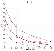
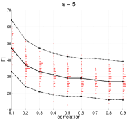
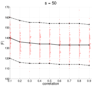
Proposition 2 asserts that conditional on having the support of included in the active set, the distribution of its cardinality is plus an extra term, whose distribution depends on that of the random variables and a ’threshold’ . In order to better understand the role of these quantities, let us first consider the case , i.e. orthonormal design: since , the distribution of is equal to plus the distribution of the number of non-negative components of a -dimensional Gaussian random vector, i.e. a binomial distribution with trials and a probability of success of (cf. also Section 2.2). Once , the distribution of gets shifted towards , noting that forms a non-increasing sequence. Specifically, for , , i.e. the larger the correlation , the stronger the concentration of the distribution of near zero. The threshold is decreasing in , i.e. the number of extra variables increases with . While the distribution of is not directly accessible, it can be approximated arbitrarily well by Monte Carlo simulation for given , and (note that the distribution does not depend on the scale of the noise ). Figure 2 depicts the -quantiles of the distribution of in virtue of (5.6) for and various choices of and . The results are based on Monte Carlo simulations for each value of . For comparison, for each pair , we generate 100 datasets with according to the model of Proposition 2 with standard Gaussian noise (the components of are set to the given lower bound on in to ensure that the event has probability close to one). We then solve the corresponding NNLS problems using the active set algorithm of Lawson and Hanson [29] and obtain the cardinalities of the active sets. Figure 2 shows a strong agreement of the predictions regarding the size of the active set based on the distribution of Proposition 2 and the empirical distributions.
 |
 |
 |
Non-negative random designs with equi-correlation structure.
We now consider random design matrices whose population Gram matrix is that of equi-correlated design, but with the possibility that . It is investigated to what extent these random design matrices inherit properties from the population setting studied in the previous paragraph. Specifically, we consider the following ensemble of random matrices
| (5.7) |
All random designs from the class share the property that the population Gram matrix possesses equi-correlation structure after re-scaling the entries of by a common factor. Denoting the mean of the entries and their squares by and , respectively, we have
such that re-scaling by leads to equi-correlation structure
with parameter . Since applications of NNLS predominantly
involve non-negative design matrices, it is instructive to have a closer
look at the class (L.5) as a basic model for such designs. Among
others, the class of sub-Gaussian random designs on encompasses the
zero-truncated Gaussian distribution, all
distributions on a bounded subset of , e.g. the family of beta
distributions (with the uniform distribution as special case) on ,
Bernoulli distributions on or more generally multinomial distributions on
positive integers , as well as any finite mixture of these distributions.
As shown in the sequel, the class (L.5) provides instances of
designs for which Theorems 2 to Theorems 4
yield meaningful results in the setting. Our reasoning hinges on both
theoretical analysis providing bounds on the deviation from population
counterparts as well as on numerical results.
Self-regularizing property + restricted eigenvalue condition of
Theorem 2.
Recall that Theorem 2 requires a combination of the
self-regularizing property (Condition 1) and the restricted
eigenvalue condition (Condition 2) to be satisfied. This turns out
to be the case for designs from in light of he following proposition. The
statement relies on recent work of Rudelson and Zhou [39]
on the restricted eigenvalue condition for random matrices with
independent sub-Gaussian rows.
Proposition 3.
Let be a random matrix from (L.5) scaled such that for some . Set . There exists constants depending only on , and the sub-Gaussian parameter of the centered entries of so that if , then, with probability at least , has the self-regularizing property with and satisfies the restricted eigenvalue condition of Theorem 2 with .
Scaling of .
The next proposition controls the deviation of the separating hyperplane
constant from its population counterpart as derived in
(5.5).
Proposition 4.
Let be a random matrix from (L.5) scaled such that for some . Fix , . Then there exists constants depending only on and the sub-Gaussian parameter of the centered entries of such that for all ,
with probability no less than .
|
|
|
|
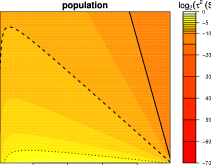
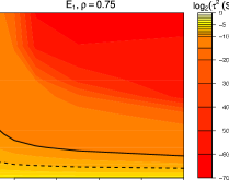
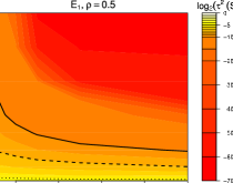
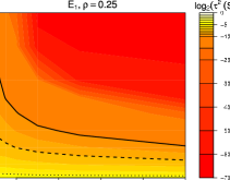
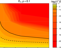
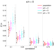
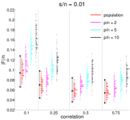
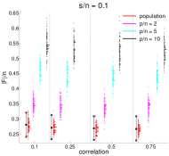
It turns out that the requirement on the sample size as indicated by Proposition 4 is too strict in light of the results of complementary numerical experiments. For these experiments, is kept fixed and and vary. For each combination of and several representatives of (re-scaled such that the population Gram matrix has equi-correlation structure), 100 random design matrices are generated. We set , compute using a QR decomposition of and then solve the quadratic program with value by means of an interior point method [6]. As representatives of , we have considered matrices whose entries have been drawn from the following distributions. In order to obtain population Gram matrices of varying correlation , we use mixture distributions with one of two mixture components being a point mass at zero (denoted by ). Note that the larger the proportion of that component, the smaller .
-
:
, ()
-
:
()
-
:
, ()
-
:
, ()
For space reasons, we here only report the results for . Regarding to , the reader is referred
to the supplement; in brief, the results confirm
what is shown here. Figure 3 displays
the 0.05-quantiles of over sets of 100 replications. It is
revealed that for to be positive, does not need to be as large
relative to as suggested by Proposition 4. In fact, even for
as large as , is sufficiently bounded away from zero as
long as is not dramatically larger than ().
Implications for compressed sensing-type problems.
In compressed
sensing (CS) [15, 13], the goal is to recover a sparse
vector from a limited number of non-adaptive measurements. In the
typical setup, the measurements are linear combinations of ,
contaminated with additive noise and thus fall under the linear model
(1.1). CS is related to group testing
[20, 21]. Here, indicates the
presence of a certain attribute of low prevalence in objects, e.g.
presence of a rare disease in individuals or of a defect in manufactured
goods. An effective strategy for locating the affected entities is by
forming groups, testing for prevalence at the group level, discarding
groups with a negative test result, and repeating the procedure with
a new set of groups. The measurements obtained in this way are both
adaptive and non-linear and hence do not fit into the conventional framework
of CS. However, this is the case if it is possible to obtain aggregate
measurements (i.e. sums) over arbitrary groups. As exemplified in
Figure 4, the information of interest can be retrieved from few
aggregated measurements and the associated group assignments. Proper
measurement design needs to achieve a proper amount of overlapping of the
groups. In fact, it is not possible to recover from a reduced
number of measurements involving only disjoint groups. At the same time,
overlapping has to be limited to ensure that collections of columns
of the measurement matrix are linearly independent; otherwise, recovery
of is not possible in general. Without further prior knowledge,
about the location of the non-zero entries of , random group
assignments in which each entity , , is assigned to
group , , independently with probability , appears
to be reasonable in light of the results of the previous paragraph.
Propositions 3 and 4 assert
that, with high probability, the resulting measurement matrix suits well a
sparse recovery approach based on NNLS.
Network tomography as discussed in [34] arises
as a generalization of the above setting with measurements of the
form , where represents the
measurement design and is the adjacency matrix
of the nodes whose status of interest is contained in . The goal is to spot sources of anomaly within the network. As
distinguished from a random design setting, the measurement matrix
cannot be chosen freely, since is fixed and the choice of
is subject to various constraints. Therefore, it is not clear a priori
whether satisfies our conditions, even though is potentially self-regularizing as is non-negative.
Sparsity of the solution.
In Proposition 2, we have characterized the sparsity
in the population setting. It is of interest to investigate this aspect for
random design in the setup, particularly in light of Theorem
4, which implicitly relies on having a sparse NNLS
solution. We here provide a sketch of the empirical behaviour within the
experimental framework of the previous paragraph. We generate random design
matrices (, ) from for the four values of
the parameter as given above. For several values of ranging from
to , we generate observations , where is a Gaussian noise
vector, and the components of are set to the lower bound in
Proposition 2. For each
combination of , 100 replications are considered and the
fraction of active variables is determined.
 |
 |
 |
 |
 |
 |
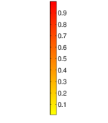
Figure 5 summarizes the main findings of this experimental study. For fixed , the top panel depicts the empirical distributions of over the 100 replications in comparison to the population setting (cf. Figure 2). We observe that for all parameter configurations under consideration, the cardinalities of the active sets stay visibly away from with being no larger than . The cardinalities of the active sets are larger than in the population case. The higher the sparsity level and the ratio , the more pronounced the shifts toward larger cardinalities: while for and , the empirical distribution of is rather close to that of the population, there is a consistent gap for . The bottom panel displays how scales with . For plotting and space reasons, we restrict us to the -quantiles over the 100 replications and , which, as indicated by the plots of the top panel, is the worst case among all values of considered. The two surface plots for and are of a similar form; a noticeable difference occurs only for rather small . It can be seen that for fixed, roughly remains constant as varies. On the other hand, increases rather sharply with . For , we observe a breakdown, as . We point out that as long as , it holds that the NNLS solution and the active set are unique (with probability one), as follows from Lemma 5 in Appendix G.
6 Empirical performance
We here present the results of simulation studies in order to compare the performance of NNLS and the non-negative lasso in terms of prediction, estimation and sparse recovery.
6.1 Deconvolution of spike trains
We consider a positive spike-deconvolution model as in [30], as it commonly appears in various fields of applications. The underlying signal is a function on of the form
with , , where is given and the ’s define the locations of the spikes contained in . The amplitudes are assumed to be positive. The goal is to determine the positions as well as the amplitudes of the spikes from (potentially noisy) samples of the underlying signal . As demonstrated below, NNLS can be a first step towards deconvolution. The idea is to construct a design matrix of the form , where for candidate positions placed densely in and are the points at which the signal is sampled. Under an additive noise model with zero-mean sub-Gaussian noise , i.e.
| (6.1) |
and if has the self-regularizing property (cf. Section 2), it follows immediately from Theorem 1 that the -prediction error of NNLS is bounded as
| (6.2) |
where . Even though it is not realistic to assume that , i.e. that the linear model is correctly specified, we may think of being negligible as long as the are placed densely enough. This means that NNLS may be suitable for de-noising. Furthermore, the bound (6.2) implies that must have large components only for those columns of corresponding to locations near the locations of the spikes, which can then be estimated accurately by applying a simple form of post-processing as discussed in [42]. On the other hand, the application of fast rate bounds such as that of Theorem 2 or corresponding results for the lasso is not adequate here, because the dense placement of the results into a tiny, if not zero, value of the restricted eigenvalue of Condition 2.
 |
 |
For our simulation study, we consider model (6.1) as starting point. The signal is composed of five spikes of amplitudes between and convolved with a Gaussian function. The design matrix contains evaluations of Gaussians at points , where both the centers of the as well as the are equi-spaced in the unit interval. We have by construction that so that . The standard deviation of the Gaussians is chosen such that it is roughly twice the spacing of the . At this point, it is important to note that the larger the standard deviations of the Gaussians, the larger the constant (2.2), which here evaluates as . According to that setup, we generate 100 different vectors resulting from different realizations of the noise whose entries are drawn i.i.d. from a Gaussian distribution with standard deviation . The left panel of Figure 6 visualizes the setting. We compare the performance of NNLS, lasso/non-negative lasso with (i) fixed regularization parameter fixed to (ii) chosen from the grid by tenfold cross-validation, ridge regression (tuned by tenfold cross-validation) and an oracle least squares estimator based on knowledge of the positions of the spikes. The right panel of Figure 6 contains boxplots of the MSEs over all 100 replications. The performance of NNLS is only slightly inferior to that of the non-negative lasso, which is not far from the oracle, and roughly as good as that of the lasso. All methods improve substantially over ridge regression. The lower part of the left panel provides a summary of the NNLS estimator , which is remarkably sparse and concentrated near the positions of the underlying spikes.
6.2 Sparse recovery
We now present the results of simulations in which we investigate the
performance of NNLS with regard to estimation and sparse recovery in
comparison to that of the non-negative lasso.
Setup. We generate data , where has i.i.d. standard Gaussian
entries. For the design , two setups are considered.
Design I: Equi-correlation like design.
The matrix is generated by drawing its entries independently from the
uniform distribution on and rescaling them such that the population
Gram matrix is of equi-correlation structure with . Random matrices of
that form have been considered for the numerical results in Section
5.3 (cf. Figures 2 to 5). For given
, the target is generated by setting , , where
denotes the smallest eigenvalue of the population Gram
matrix, the are drawn uniformly from , and we let
the parameter vary. We further set , .
Design II: Localized non-negative functions.
The setup leading to the second class of designs can be regarded as a
simplification of the deconvolution problem discussed in
the previous subsection to fit into the standard sparse recovery
framework. Indeed, in the experiments of Section 6.1,
recovery of the support of fails in the presence of noise, because the
’s are placed too densely relative to the number of sampling
points; see [11] for a similar discussion concerning the
recovery of mixture components in sparse mixture density estimation. In order
to circumvent this issue, we use the following scheme. As in Section
6.1, we consider sampling points ,
, in and localized functions ,where here ,
with . The centers , , are taken from the interval
, where and . Given the sparsity level , is
partitioned into sub-intervals of equal length and the centers
corresponding to are drawn from the uniform distributions on these
intervals. The remaining centers corresponding to
are drawn uniformly from , where is set to enforce a
sufficient amount of separation of the from the . We here choose . The design matrix
is then of the form , ,
, where the ’s are scaling factors such that . As
for Design I, we generate observations , where , and , . The are random variables from the uniform distribution on and
the choice
has turned out to yield sufficiently challenging problems.
For both Design I and II, two sets of experiments are performed. In the first
one, the parameter controlling the magnitude of the coefficients of the
support is fixed to (Design I) respectively (Design II) , while the aspect ratio of and the
fraction of sparsity vary. In the second set of experiments,
is fixed to (Design I) and (Design II), while and
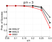
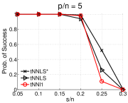
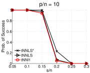
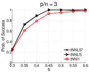
vary. Each configuration is replicated 100 times for .
Comparison. Across these runs, we compare thresholded NNLS, the non-negative lasso (NN), the thresholded non-negative
lasso (tNN) and orthogonal matching pursuit (OMP, [48, 58])
with regard to their performance in sparse recovery. Additionally, we compare
NNLS and NN with as defined below (both
without subsequent thresholding) with regard to
estimation of in -norm (Tables
1 and 2) and
-norm (the results are contained in the supplement).
The performance of thresholded NNLS with regard to sparse recovery is assessed in two
ways. For the first one (referred to as ’tNNLS∗’), success is reported whenever , i.e. there exists a
threshold that permits support recovery. Second, the procedure of Theorem
5 (with replaced by the naive estimate
) is used to determine the threshold in a data-driven
manner without knowledge of . This approach is referred to as tNNLS. For tNN, both the regularization parameter
and the threshold have to be specified. Instead of fixing to a single value, we
give tNN a slight advantage by simultaneously considering all solutions prior to thresholding,
where equals the choice of the regularization parameter advocated in
[5] to achieve the optimal rate for the estimation of
in the -norm and can be interpreted as
empirical counterpart to . The non-negative lasso modification of LARS
[22] is used to obtain the solutions
; we
then report success of tNN whenever holds for at least one of these solutions. We
point out that specification of is based on knowledge of the noise
variance, which constitutes a second potential advantage for tNN.
Under the conditions of Theorem 6, NN recovers the support
directly without thresholding. In order to judge the usefulness
of subsequent thresholding of NN, we obtain as well the set of
non-negative lasso solutions and check whether the sparsity pattern of any of these
solutions recovers .
Given its simplicity, OMP serves as basic reference
method. Success is reported whenever the
support has been recovered after steps.
 |
 |
 |
 |
 |
 |
 |
 |
 |
 |
 |
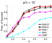 |
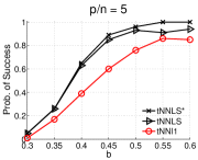
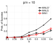
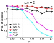
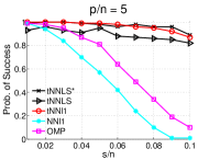
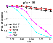
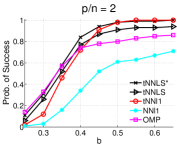
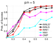
Discussion of the results. In summary, Figures 7 and 8 indicate that for the two setups under consideration, NNLS and its thresholded version exhibit excellent performance in sparse recovery. A superior performance relative to the thresholded non-negative lasso is achieved particularly in more difficult parameter regimes characterized by comparatively small signal strength or high fraction of sparsity. The results of the experiments reveal that the non-negative lasso without thresholding may perform well in estimation, but it is not competitive as far as sparse recovery is concerned. This observation is in agreement with existing literature in which the restrictiveness of the conditions for the lasso to select the correct set of variables is pointed out and two stage procedures like thresholding are proposed as remedy [63, 36, 59, 62, 49]. At this point, we stress again that NNLS only requires one parameter (the threshold) to be set, whereas competitive performance with regard to sparse recovery based on the non-negative lasso entails specification of two parameters. Let us now give some more specific comments separately for the two designs. For Design I, thresholded NNLS visibly improves over tNN, predominantly even in case that the threshold is chosen adaptively without knowledge of . For Design II, noticeable differences between tNNLS∗ and tNN occur for small values of . Apart from that, the performance is essentially identical. Even though the results of tNNLS remain competitive, they fall behind those of tNNLS∗ and tNN. OMP partially keeps up with the other methods for and/or small, while NN succeeds as well in a substantial fraction of cases for small . This is to be contrasted with the situation for Design I, in which both OMP and NN do not even achieve success in a single trial. This outcome is a consequence of the fact that the non-negative irrepresentable condition (cf. Section 4.4), which is necessary for the success of OMP as well [58], fails to hold in all these runs. The -errors in estimating reported in Tables 1 and 2 are in accordance with the sparse recovery results. The smaller and , the closer NNLS and NN are in performance. An advantage of NNLS arises for more extreme combinations of . A similar conclusion can be drawn for the -errors (cf. supplement).
| nnls | nn | nnls | nn | |
| .34.005 | .34.005 | .35.005 | .36.005 | |
| .37.005 | .37.005 | .41.005 | .40.005 | |
| .41.006 | .42.009 | .44.005 | .46.012 | |
| .43.006 | .46.012 | .50.007 | .56.023 | |
| .48.006 | .54.020 | .58.009 | .72.030 | |
| .55.007 | .64.027 | .70.012 | 1.01.04 | |
| nnls | nn | nnls | nn | |
| .37.005 | .38.005 | .43.006 | .43.006 | |
| .44.005 | .45.006 | .51.007 | .52.007 | |
| .52.007 | .54.007 | .66.009 | .71.012 | |
| .61.008 | .66.009 | 1.01.02 | 1.28.03 | |
| .81.014 | 1.32.04 | 1.91.02 | 2.17.02 | |
| 1.36.03 | 1.90.03 | 2.32.02 | 2.36.03 | |
| nnls | nn | nnls | nn | |
| .20.005 | .32.005 | .21.005 | .32.005 | |
| .23.004 | .34.004 | .24.007 | .35.006 | |
| .25.006 | .36.005 | .27.008 | .37.006 | |
| .28.010 | .37.009 | .28.009 | .37.006 | |
| .29.010 | .37.007 | .32.012 | .39.010 | |
| nnls | nn | nnls | nn | |
| .21.004 | .32.004 | .22.005 | .33.006 | |
| .23.005 | .34.004 | .24.005 | .35.005 | |
| .27.005 | .36.005 | .27.006 | .37.006 | |
| .29.011 | .37.009 | .30.009 | .37.006 | |
| .32.011 | .40.010 | .32.011 | .39.008 | |
Acknowledgements
We would like to thank Mike Davies, Rolf Schneider, Jared Tanner and Roman Vershynin for helpful discussions. We thank the Editor and the reviewers for thorougly reading the manuscript and providing valuable comments and suggestions. We are also indebted to a reviewer of an earlier draft, whose comments prompted us to organize Section 3 in its present form.
Appendix A Standard tail bounds for sub-Gaussian random variables
A zero-mean random variable is called sub-Gaussian if there exists (referred to as sub-Gaussian parameter) so that the moment-generating function obeys the bound . It follows that if are i.i.d. copies of and , then is sub-Gaussian with parameter . We have the well-known tail bound
| (A.1) |
Combining the previous two facts and using a union bound with it follows that for any collection of vectors , ,
| (A.2) |
To obtain the main results of the paper, (L.1) is applied with and under the assumption , , , and the choice for , which yields
| (A.3) |
Appendix B Proof of Proposition 1
Since satisfies Condition 1, by (2.2), there exists a unit vector so that
| (B.1) |
for some constant . Setting as the projection on the subspace orthogonal to , the least squares objective can be decomposed as follows.
where . In the last line, we have invoked the assumptions made for . Writing for the diagonal matrix with the entries of on its diagonal and setting and , we have
where we have used (B.1). Note that by (B.1) and , has the property claimed in the statement. In view of the presence of the term , any minimizer of the r.h.s. must obey . As a result,
which finishes the proof of the first claim of the proposition. To establish the second claim, observe that any satisfies
Expanding the square and re-arranging, we obtain
As established above, , so that as long as .
Appendix C Proof of Theorem 1
Since is a minimizer of the NNLS problem (1.2) and since is a feasible solution, we have that
| (C.1) | ||||
Write , and . We now lower bound using the self-regularizing property of Condition 1 according to (2.3).
| (C.2) | ||||
Second, we bound the r.h.s. of (C.1). We set and use the bound
obtaining that
| (C.3) |
Inserting the lower bound (C.2) into (C.3), we obtain
| (C.4) |
We may assume that , otherwise the assertion of the theorem would follow immediately, because is already bounded for feasibility reasons, see below. Dividing both sides by and re-arranging yields
| (C.5) |
where we have assumed that (if that were not the case, one would obtain , which is stronger than (C.5), since ). We now substitute (C.5) back into (C.1) and add to both sides of the inequality in order to obtain
noting that by feasibility of , one has and hence . Using (A.3), the event holds with probability no less than . The result follows.
Appendix D Proofs of Lemma 1 and Theorem 2
We build on ideas already used in the proof of Theorem 1. In particular, all notations introduced in the previous proof are adopted. First note that and . Hence, we obtain the following analog to (C.4).
Dividing both sides by , assuming that (otherwise, the claim as in the first event of Lemma 1 would follow trivially), we obtain
If , then the first event of Lemma
1 occurs. Otherwise, we conclude that the second event of
Lemma 1 occurs by applying (A.3)
to bound as in the proof of Theorem 1.
In the latter case, the assertion of Theorem 2 follows
immediately. Thus, the rest of the proof is conditional on the first event.
In terms of Condition 2, , so
that one may invoke the restricted eigenvalue condition (L.18),
which, when applied to (C.1), yields
which implies that
The preceding bound in turn implies
Controlling as above, the -bound and the bound on the prediction error follow. The bound on for can be established similarly. The proof is along the lines of the proof of Theorem 7.2 in [5] and is hence omitted.
Appendix E Proof of Lemma 2
The proof of the lemma relies on the following auxiliary result, which is immediate from the KKT optimality conditions of the NNLS problem. Its proof is hence omitted.
Lemma 3.
is a minimizer of the NNLS problem (1.2) if and only if there exists such that
Lemma 3 implies that any NNLS solution is a minimizer of a least squares problem subject to the equality constraint given the active set , that is
Proof of Lemma 2. The NNLS objective can be split into two parts as follows.
| (E.1) |
Separate minimization of the second summand on the r.h.s. of (E.1) yields . Substituting for in the first summand, and minimizing the latter amounts to solving . In view of Lemma 3, if , it coincides with an unconstrained least squares estimator corresponding to problem . This implies that the optimal value of must be zero, because the observation vector of the non-negative least squares problem is contained in the column space of . Since the second summand in (E.1) corresponding to cannot be made smaller than by separate minimization, we have minimized the non-negative least squares objective.
Appendix F Proof of Theorem 3
We here state and prove a result that is slightly more general than Theorem 3, as it covers also the case of an approximately sparse target. Writing for the sequence of ordered coefficients, let be the set of the largest coefficients of (for simplicity, assume that there are no ties). For the result that follows, we think of being considerably smaller than the entries of .
Theorem 7.
Consider the linear model , where and has i.i.d. zero-mean sub-Gaussian entries with sub-Gaussian parameter . For , set
| and |
If , then the NNLS estimator has the following properties with probability no less than :
The special case of exact sparsity in which equals the support of is obtained for (cf. Theorem 3).
Proof.
First note that in the more general case with , an analog of Lemma 2 holds with
Consider problem .
Step 1: Controlling via
. Since is a minimizer and is feasible
for , we have
which implies that
| (F.1) | ||||
In the last inequality, we have used that for all , it holds that
| (F.2) |
As observed in (4.3), , s.t. the l.h.s. of (F.1) can be lower bounded via
| (F.3) |
Combining (F.1) and (F.3), we have
.
Step 2: Back-substitution into (P2). Equipped with the bound
just derived, we insert into problem of Lemma 2,
and show that in conjunction with the assumptions made for the minimum
support coefficient , the ordinary least squares
estimator corresponding to ()
has only positive components. Lemma 2 then yields . Using the closed form expression for the ordinary least squares estimator, one obtains
| (F.4) | ||||
It remains to control the two terms and . For the second term, we have
| (F.5) | ||||
Step 3: Putting together the pieces. The two random terms and are maxima of a finite collection of linear combinations of sub-Gaussian random variables so that (L.1) in Appendix A can be applied by estimating Euclidean norms. For , we use (F.2). Second, we have
| (F.6) |
where denotes the -th canonical basis vector. One has
It follows that for any the event
holds with probability no less than . Conditional on that event, it follows that with as in Theorem 3, we have
and hence, using the lower bound on , that and thus also that . ∎
Appendix G Proof of Theorem 4
Part 1: proof of uniqueness.
To prove the first part of the theorem asserting uniqueness of the NNLS solution, we need two additional lemmas. The first one is a concentration result which is a special case of Theorem 2.5 in [28].
Lemma 4.
Let be a projection matrix on a -dimensional subspace of and let be a random vector whose entries are i.i.d. zero-mean sub-Gaussian random variables with parameter . Then
where is a universal constant.
The second lemma provides two sufficient conditions for the NNLS solution to be unique.
Lemma 5.
Let the columns of be in
general linear position. Then the NNLS problem
has a unique solution if one of the following holds:
(i) , (ii) .
Moreover, under (ii) the active set satisfies . Conversely,
if has a distribution that is absolutely continuous with respect to the
Lebesgue measure, then implies with probability one
that the NNLS problem has a unique solution.
Proof.
Suppose that (i) holds. The fact that the columns of are in general linear position implies that is strictly positive definite so that the NNLS objective is strictly convex and hence has a unique minimizer. We now turn to the case . We first note that is unique, because it is the projection of onto the polyhedral cone , which is a convex set. Moreover, under (ii), must be contained in the boundary of (by general linear position, the interior of is non-empty). Note that equals the union of the facets of , that is
From , it hence follows that the active set has cardinality at most . General linear
position implies that the linear system has exactly
one solution .
Concerning the second part of the lemma, the assertion is
trivial for . Conversely, if , the fact that allows us to conclude that
so that the assertion follows from the reasoning above. For the third part, we
note that the fact that has a distribution which is absolutely continuous
with respect to the Lebesgue measure implies that is not contained in any
subspace of dimension smaller than with probability one, so that
, and the claim
follows from part (ii).
∎
Using Lemma 5 and the condition (4.7)
we will show that for , condition (ii) of Lemma 5 holds with the stated probability, from which we will conclude the proof of the first part of the theorem. Note that for , uniqueness follows from general linear position while the claim is trivial. Let us recall the decomposition of Lemma 2. Note that
hence it suffices to show that the right hand side is strictly positive. Suppose conversely that , then . Since is a minimizer of , , which, by the definition of , implies that
and in turn
Hence, conditional on the event
| (G.1) |
it holds that
which contradicts (4.7). As a result, as was to be shown. Invoking Lemma 4 with so that by general linear position and treating the second event in (G.1) as in step 3 of Appendix F, the probability of the event (G.1) is no less than .
Part 2: proof of the bound on .
Given uniqueness of the NNLS solution and in turn of its active set , the stated bound on follows readily once it holds that . In fact, the optimality conditions of the NNLS problem (cf. Lemma 3) then yield that can be recovered from the linear system
where the second equality results from . As an immediate consequence, we have that
In order to control the random term, we may follow the reasoning below (F.6) to conclude that for any , the event
has probability at least . It remains to show that under the conditions of the theorem, we indeed have that . This is done by referring to the scheme in Appendix F . Given the lower bound on , it is established that the event and in turn occurs with probability at least . This finishes the proof.
Appendix H Proof of Theorem 5
We first recall that the analysis is conditional on the event
| (H.1) |
Our proof closely follows the corresponding proof in [23]. We show in two steps that both and . For both steps, we shall need the following observations. Let denote the linear space spanned by the top variables according to the given ranking, , and let . Let further , , which are subspaces of of dimension at most . In case that the dimension of is one, let be the unit vector spanning and let otherwise, . Note that as appearing in the definition of the ’s equals the projection on the , . In particular, we have
| (H.2) |
Step 1: no false negatives
In the sequel, let denote the threshold of the procedure so that
Later in the proof, it will be verified that can be chosen as asserted in the theorem. We first note that conditional on , by definition of , it holds that the event is contained in the event . Hence it suffices to upper bound the probability of the event . We have
| (H.3) | ||||
where and denote the projection on the linear spaces spanned by the columns of corresponding to respectively , . In order to obtain the second inequality, we have used again that we work conditional on the event . As will be established at the end of the proof, we further have
| (H.4) |
Combining (H.3) and (H.4), it suffices to upper bound
| (H.5) |
as will be done below after fixing .
Step 2: no false positives
Conditional on , the probability of having a false positive selection is upper bounded as
| (H.6) |
Choosing for an arbitrary , using the assumption on , and controlling according to (L.1) in the usual way, the probabilities (H.5) and (H) do not exceed . The assertion of the theorem then follows. To conclude the proof, it remains to establish (H.4). Let us fix an arbitrary . We have
Write for the vector of regression coefficients for the linear regression of on , i.e.
and note that, according to a block decomposition of the matrix
We conclude the proof from and
Appendix I Proof of Theorem 6
Consider the non-negative lasso problem (1.3). It follows from the KKT optimality conditions that any minimizer of (1.3) satisfies
| (I.1) | ||||
Following the technique employed in [53], we establish that under the conditions of the theorem, the unique minimizer of the non-negative lasso problem is given by and with the specified probability, where denotes the minimizer of the following constrained non-negative lasso problem
| (I.2) |
To this end, in view of (I.1), it suffices to show that the following system of inequalities is satisfied
| (I.3) |
In view of the required lower bound on in (4.14), we have
| (I.4) |
with probability at least , handling the random term as (F.6) in the proof of Theorem 3. Substituting (I.4) back into (I.3), we find that the following system of inequalities must hold true:
| (I.5) |
In light of the maximal inequality (L.1), the event
| (I.6) |
occurs with probability at least , noting that for all . Hence, conditional on the events and (I.6), each component of the left hand side of (I.5) is no larger than (cf. definition (4.12)), so that for , the system of inequalities (I.5) and hence also (I.3) are indeed fulfilled.
Appendix J Example of a design for which the non-negative lasso performs sub-optimally
As indicated in the discussion following Theorem 6, the non-negative lasso does not always attain the optimal rate for estimating with respect to the -norm. For the data-generating model of Theorem 6 we give an example of a design so that the non-negative lasso estimator has the property
| (J.1) |
with high probability, provided the regularization parameter (as conventionally suggested in the literature) and the minimum support coefficient . For the same design, if , the NNLS estimator obeys the bound
| (J.2) |
with high probability. In order to establish (J.1), we shall build on the scheme used for the proof of Theorem 6 in the previous paragraph. Consider a design whose Gram matrix is of the form
where
The constant in the denominator is chosen for convenience; any other constant larger than would do as well. Using Schur complements, one computes that
As a result, we have that
| (J.3) |
where is the first canonical basis vector. Furthermore, the sequence of eigenvalues of (ordered decreasingly) is given by
From the proof of Theorem 6, we know that given the active set , the non-negative lasso estimator has the following closed form expression.
| (J.4) |
If , the claim (J.1) follows trivially from the assumption . Conversely, if , (J.4) and the block structure of imply that
using (J.3) and the maximal inequality (L.1) to upper bound the
second term after the third inequality. The latter scales as with
probability at least . Furthermore, we have used that
and .
Regarding the upper bound (J.2) for NNLS, we note
that the optimality conditions of the NNLS problem (Lemma 3)
in conjunction with the block structure of imply that
with probability at least , provided exceeds the bound on the right hand side. Similarly,
with probability at least , so that (J.2) follows.
Appendix K Proof of Proposition 2
We start by noting that is strictly positive definite so that the NNLS problem is strictly convex. Thus, the NNLS solution and its active set are unique. Let us first consider the case . Using a slight modification of the scheme used in the proofs of Theorem 3 and 4, we will show that under the required condition on , the event holds with the stated probability, which proves the first statement of the proposition. Following the proof of Theorem 3, we have that
with probability at least , where we have used the closed form expression for in (5.5). In order to verify that , we follow the back-substitution step (step 2 in Appendix F) apart from the following modification. In place of (F.5), we bound
For the first equality, we have used that and the fact that the matrix has constant entries equal to . For the second inequality, we have used that is an eigenvector of corresponding to its largest eigenvalue . Turning to step 3 in Appendix F, we note that with ,
so that with probability at least as claimed.
We now turn to the second statement of the proposition concerning the
(conditional) distribution of the cardinality of the active set.
Conditional on the event , the KKT optimality conditions of the NNLS
problem as stated in Lemma 3 imply that the following block system of
inequalities holds.
| (K.1) |
Resolving the top block for , we obtain
Back-substituting that expression into the bottom block of inequalities yields the following system of inequalities.
| (K.2) |
where . For equi-correlated design with , we have that
| (K.3) |
cf. the derivation in (5.5). Denote , and . Using Lemma 3 and (K.3), (K.2) can be written as
| (K.4) | ||||
Set so that is a zero-mean Gaussian random vector with covariance
In view of (K.3), has the distribution as claimed in Proposition 2. From (K.4), we conclude that
| (K.5) |
In particular, recalling that denotes the arrangement of the components of in decreasing order, if , then (K.4) implies that , and as stated in the proposition. Let us henceforth assume that , in which case (K.4) implies that is non-empty. We may then resolve the first set of equations in (K.4) with respect to , which yields
where the second equality is an application of the Sherman-Woodbury-Morrison formula. This implies in turn that
Substituting this expression back into (K.4), we obtain
| (K.6) | ||||
Now note that for ,
From
(K.5) and the inequalities in (K.6), it then follows that
where is the largest integer so that with as defined in (5.6), which finishes the proof for . Turning to the case , a similar scheme can be used, starting from the system of inequalities . The expressions used above remain valid with .
Appendix L Proof of Propositions 3 and 4
References
- and. Z. Guo and Osher [2010] A. Szlam and. Z. Guo and S. Osher. A split Bregman method for non-negative sparsity penalized least squares with applications to hyperspectral demixing. In IEEE International Conference on Image Processing, 2010.
- Bardsley and Nagy [2006] J. Bardsley and J. Nagy. Covariance-preconditioned iterative methods for nonnegatively constrained astronomical imaging. SIAM Journal on Matrix Analysis and Applications, 27:1184–1198, 2006.
- Bartlett et al. [2012] P. Bartlett, S. Mendelson, and J. Neeman. -regularized linear regression: Persistence and oracle inequalities. Probability Theory and Related Fields, 254:193–224, 2012.
- Belloni et al. [2011] A. Belloni, V. Chernozukov, and L. Wang. Square root lasso: Pivotal recovery of sparse signals via conic programming. Biometrika, 98:791–806, 2011.
- Bickel et al. [2009] P. Bickel, Y. Ritov, and A. Tsybakov. Simultaneous analysis of Lasso and Dantzig selector. The Annals of Statistics, 37:1705–1732, 2009.
- Boyd and Vandenberghe [2004] S. Boyd and L. Vandenberghe. Convex Optimization. Cambridge University Press, 2004.
- Bruckstein et al. [2008] A. Bruckstein, M. Elad, and M. Zibulevsky. On the uniqueness of nonnegative sparse solutions to underdetermined systems of equations. IEEE Transactions on Information Theory, 54:4813–4820, 2008.
- Bühlmann and van de Geer [2011] P. Bühlmann and S. van de Geer. Statistics for high-dimensional data. Springer, 2011.
- Bunea [2008] F. Bunea. Honest variable selection in linear and logistic regression models via and penalization. The Electronic Journal of Statistics, 2:1153–1194, 2008.
- Bunea et al. [2007] F. Bunea, A. Tsybakov, and M. Wegkamp. Sparsity oracle inequalities for the lasso. The Electronic Journal of Statistics, 1:169–194, 2007.
- Bunea et al. [2010] F. Bunea, A. Tsybakov, M. Wegkamp, and A. Barbu. SPADES and mixture models. The Annals of Statistics, 38:2525–2558, 2010.
- Candes and Plan [2009] E. Candes and Y. Plan. Near-ideal model selection by -minimization. The Annals of Statistics, 37:2145–2177, 2009.
- Candes and Tao [2007] E. Candes and T. Tao. The Dantzig selector: statistical estimation when is much larger than . The Annals of Statistics, 35:2313–2351, 2007.
- Chen and Plemmons [2007] D. Chen and R. Plemmons. Nonnegativity constraints in numerical analysis. In Symposium on the Birth of Numerical Analysis, 2007.
- Donoho [2006] D. Donoho. Compressed sensing. IEEE Transactions on Information Theory, 52:1289–1306, 2006.
- Donoho and Tanner [2005a] D. Donoho and J. Tanner. Sparse nonnegative solution of underdetermined linear equations by linear programming. Proceedings of the National Academy of Science, 102:9446–9451, 2005a.
- Donoho and Tanner [2005b] D. Donoho and J. Tanner. Neighbourliness of randomly projected simplices in high dimensions. Proceedings of the National Academy of Science, 102:9452–9457, 2005b.
- Donoho and Tanner [2010] D. Donoho and J. Tanner. Counting the faces of randomly-projected hypercubes and orthants, with applications. Discrete and Computational Geometry, 43:522–541, 2010.
- Donoho et al. [1992] D. Donoho, I. Johnstone, J. Hoch, and A. Stern. Maximum entropy and the nearly black object. Journal of the Royal Statistical Society Series B, 54:41–81, 1992.
- Dorfman [1943] R. Dorfman. The detection of defective members of large populations. The Annals of Mathematical Statistics, 14:436–440, 1943.
- Du and Hwang [2006] D. Du and F. Hwang. Pooling Designs and Nonadaptive Group Testing. Twayne Publishers, 2006.
- Efron et al. [2004] B. Efron, T. Hastie, I. Johnstone, and R. Tibshirani. Least Angle Regression. The Annals of Statistics, 32:407–499, 2004.
- Genovese et al. [2012] C. Genovese, J. Jin, L. Wasserman, and Z. Yao. A Comparison of the Lasso and Marginal Regression. Journal of Machine Learning Research, 13:2107–2143, 2012.
- Greenshtein and Ritov [2004] E. Greenshtein and Y. Ritov. Persistence in high-dimensional linear predictor selection and the virtue of overparametrization. Bernoulli, 6:971–988, 2004.
- Hebiri and Lederer [2013] M. Hebiri and J. Lederer. How correlations influence Lasso Prediction. IEEE Transactions on Information Theory, 59:1846–1854, 2013.
- Huet et al. [2012] S. Huet, C. Giraud, and N. Verzelen. High-dimensional regression with unknown variance. Statistical Science, 27:500–518, 2012.
- Kim et al. [2010] D. Kim, S. Sra, and I. Dhillon. Tackling box-constrained convex optimization via a new projected quasi-Newton approach. SIAM Journal on Scientific Computing, 32:3548–3563, 2010.
- Latala et al. [2007] R. Latala, P. Mankiewicz, K. Oleskiewicz, and N. Tomczak-Jaegermann. Banach-Mazur distances and projections on random subgaussian polytopes. Discrete and Computational Geometry, 38:29–50, 2007.
- Lawson and Hanson [1987] R. Lawson and C. Hanson. Solving least squares problems. SIAM Classics in Applied Mathematics, 1987.
- Li and Speed [2000] L. Li and T. Speed. Parametric deconvolution of positive spike trains. The Annals of Statistics, 28:1279–1301, 2000.
- Lin et al. [2004] Y. Lin, D. Lee, and L. Saul. Nonnegative deconvolution for time of arrival estimation. In ICASSP, 2004.
- Litvak et al. [2005] A. Litvak, A. Pajor, M. Rudelson, and N. Tomczak-Jaegermann. Smallest singular value of random matrices and geometry of random polytopes. Advances in Mathematics, 195:491–523, 2005.
- Lounici [2008] K. Lounici. Sup-norm convergence rate and sign concentration property of Lasso and Dantzig Selectors. The Electronic Journal of Statistics, 2:90–102, 2008.
- Meinshausen [2013] N. Meinshausen. Sign-constrained least squares estimation for high-dimensional regression. The Electronic Journal of Statistics, 7:1607–1631, 2013.
- Meinshausen and Bühlmann [2006] N. Meinshausen and P. Bühlmann. High-dimensional graphs and variable selection with the lasso. The Annals of Statistics, 34:1436–1462, 2006.
- Meinshausen and Yu [2009] N. Meinshausen and B. Yu. Lasso-type recovery of sparse representations for high-dimensional data. The Annals of Statistics, 37:246–270, 2009.
- Raskutti et al. [2010] G. Raskutti, M. Wainwright, and B. Yu. Restricted nullspace and eigenvalue properties for correlated Gaussian designs. Journal of Machine Learning Research, 11:2241–2259, 2010.
- Rudelson and Vershynin [2010] M. Rudelson and R. Vershynin. Non-asymptotic theory of random matrices: extreme singular values. In International Congress of Mathematics, 2010.
- Rudelson and Zhou [2013] M. Rudelson and S. Zhou. Reconstruction from anisotropic random measurements. IEEE Transactions on Information Theory, 59:3434–3447, 2013.
- Schneider and Weil [2008] R. Schneider and W. Weil. Stochastic and Integral Geometry. Springer, 2008.
- Schölkopf and Smola [2002] B. Schölkopf and A. Smola. Learning with kernels. MIT Press, Cambridge, Massachussets, 2002.
- Slawski and Hein [2010] M. Slawski and M. Hein. Sparse recovery for Protein Mass Spectrometry data. In NIPS workshop on practical applications of sparse modelling, 2010.
- Slawski and Hein [2011] M. Slawski and M. Hein. Sparse recovery by thresholded non-negative least squares. In Advances in Neural Information Processing Systems 24, pages 1926–1934. 2011.
- Slawski and Hein [2012] M. Slawski and M. Hein. Non-negative least squares for high-dimensional linear models: consistency and sparse recovery without regularization. arXiv:1205.0953v1, 2012.
- Sun and Zhang [2012] T. Sun and C-H Zhang. Scaled sparse linear regression. Biometrika, 99:879–898, 2012.
- Tibshirani [1996] R. Tibshirani. Regression shrinkage and variable selection via the lasso. Journal of the Royal Statistical Society Series B, 58:671–686, 1996.
- Tibshirani [2011] R. Tibshirani. Regression shrinkage and selection via the lasso: a retrospective (with discussion). Journal of the Royal Statistical Society Series B, 73:273–282, 2011.
- Tropp [2004] J. Tropp. Greed is good: Algorithmic results for sparse approximation. IEEE Transactions on Information Theory, 50:2231–2242, 2004.
- Tsybakov [2010] A. Tsybakov. Discussion of ’Stability Section’ by N. Meinshausen and P. Bühlmann. Journal of the Royal Statistical Society Series B, 72:467, 2010.
- van de Geer [2008] S. van de Geer. High-dimensional generalized linear models and the lasso. The Annals of Statistics, 36:614–645, 2008.
- van de Geer and Bühlmann [2009] S. van de Geer and P. Bühlmann. On the conditions used to prove oracle results for the Lasso. The Electronic Journal of Statistics, 3:1360–1392, 2009.
- van de Geer and Lederer [2012] S. van de Geer and J. Lederer. From Probability to Statistics and Back: High-Dimensional Models and Processes. A Festschrift in Honor of Jon Wellner, chapter ’The Lasso, correlated design, and improved oracle inequalities’. IMS Collections. 2012.
- Wainwright [2009] M. Wainwright. Sharp thresholds for noisy and high-dimensional recovery of sparsity using -constrained quadratic programming (Lasso). IEEE Transactions on Information Theory, 55:2183–2202, 2009.
- Wang and Tang [2009] M. Wang and A. Tang. Conditions for a Unique Non-negative Solution to an Underdetermined System. In Proceedings of Allerton Conference on Communication, Control, and Computing, 2009.
- Wang et al. [2011] M. Wang, W. Xu, and A. Tang. A unique nonnegative solution to an undetermined system: from vectors to matrices. IEEE Transactions on Signal Processing, 59:1007–1016, 2011.
- Wendel [1962] J.G. Wendel. A problem in geometric probability. Mathematics Scandinavia, 11:109–111, 1962.
- Zhang and Huang [2008] C-H Zhang and J. Huang. The sparsity and bias of the Lasso selection in high-dimensional linear regression. The Annals of Statistics, 36:1567–1594, 2008.
- Zhang [2009a] T. Zhang. On the Consistency of Feature Selection using Greedy Least Squares Regression. Journal of Machine Learning Research, 10:555–568, 2009a.
- Zhang [2009b] T. Zhang. Some Sharp Performance Bounds for Least Squares Regression with Regularization. The Annals of Statistics, 37:2109–2144, 2009b.
- Zhao and Yu [2006] P. Zhao and B. Yu. On model selection consistency of the lasso. Journal of Machine Learning Research, 7:2541–2567, 2006.
- Zhao [2012] Y-B Zhao. Sparsest and least -norm nonnegative solutions to linear systems with applications to compressive sensing and linear programs. Technical report, University of Birmingham, 2012.
- Zhou [2009] S. Zhou. Thresholding procedures for high dimensional variable selection and statistical estimation. In NIPS, 2009.
- Zou [2006] H. Zou. The adaptive lasso and its oracle properties. Journal of the American Statistical Association, 101:1418–1429, 2006.
Supplementary material to
’Non-negative least squares for high-dimensional linear
models: consistency and sparse recovery
without regularization’
Proofs of Propositions 3 and 4
We here provide proofs of Propositions 3 and 4 concerning random equi-correlation-like matrices. These proofs rely on a series of lemmas that are stated first.
Additional lemmas
We recall from Appendix A of the paper that a zero-mean random variable is called sub-Gaussian if there exists (referred to as sub-Gaussian parameter) so that the moment-generating function obeys the bound . If are i.i.d. copies of and , , are fixed vectors, then
| (L.1) |
Bernstein-type inequality for squared sub-Gaussian random variables
The following exponential inequality combines Lemma 14, Proposition 16 and Remark 18 in [4].
Lemma 1.
Let be i.i.d. zero-mean sub-Gaussian random variables with parameter and the property that . Then for any , one has
| (L.2) |
where is an absolute constant.
Concentration of extreme singular values of sub-Gaussian random matrices
Let and denote the minimum and maximum singular value of a matrix . The following lemma is a special case of Theorem 39 in [4].
Lemma 2.
Let be an matrix with i.i.d. zero-mean sub-Gaussian entries with sub-Gaussian parameter and unit variance. Then for every , with probability at least , one has
| (L.3) |
with , depending only on .
Entry-wise concentration of the Gram matrix associated with a sub-Gaussian random matrix
The next lemma results from Lemma 1 in [2] and the union bound.
Lemma 3.
Let be an random matrix of i.i.d. zero-mean, unit variance sub-Gaussian entries with parameter . Then
| (L.4) |
for all .
Application to
Recall that the class is given by
| (L.5) |
We shall make use of the following decomposition valid for any from (L.5).
| (L.6) |
where the entries of are zero mean sub-Gaussian random variables with parameter , say, and is an -matrix of ones. In the sequel, we specialize to the case where the entries of are scaled such that
| (L.7) |
for , i.e. the population Gram matrix has equi-correlation structure. Then, decomposition (L.6) becomes
| (L.8) |
Accordingly, we have the following expansion of .
| (L.9) |
Observe that
| (L.10) |
where is a diagonal matrix with diagonal entries , . It hence follows from (L.1) that
| (L.11) |
Combining (L.7), (L.9), (L.11) and Lemma 3, it follows that there exists a constant depending only on such that
| (L.12) |
Let now , be given. Without loss of generality, let us assume that . In the sequel, we control . From decomposition (L.9), we obtain that
| (L.13) |
Introduce as the vector of column means of . We have that
| (L.14) |
Moreover,
| (L.15) |
Noting that the are i.i.d. zero-mean sub-Gaussian random variables with parameter and variance no larger than one, we are in position to apply Lemma 1, which yields that for any
| (L.16) |
Combining (L.13), (L.14) and
(L.16) and using Lemma
2 to control the term
, we obtain that
for any and any
| (L.17) | ||||
where only depend on the sub-Gaussian parameter . Equipped with these auxiliary results, we now turn to the proofs of Proposition 3 and 4.
Proof of Proposition 3
Let us first recall the restricted eigenvalue condition.
Condition 2.
Let and for and ,
We say that the design satisfies the -restricted eigenvalue condition if there exists a constant so that
| (L.18) |
The proof of Proposition 3 relies on a recent result in [3]. In order to state that result, we need the following preliminaries concerning -random variables taken from [1] (see Definition 1.1.1 and Theorem 1.1.5 therein).
Definition 1.
A random variable is said to be with parameter if
| (L.19) |
Lemma 4.
If a random variable has the property that there exist positive constants so that
then is with parameter no more than .
The following statement is essentially a special case of Theorem 1.6 in [3]. We state it in simplified form that is sufficient for our purpose here.
Lemma 5.
Let be a matrix whose rows , are independent random vectors that are
-
1.
isotropic, i.e. , ,
-
2.
, i.e. there exists such that for every unit vector
(L.20)
Let further be a positive definite matrix with minimum eigenvalue and set . Then, for any and any , there exist positive constants , (the first depending on the parameter ) so that if
with probability at least , satisfies the -restricted eigenvalue condition with .
We now state and prove Proposition 3.
Proposition 3.
Let be a random matrix from (L.5) scaled such that for some . Set . There exists constants depending only on , and the sub-Gaussian parameter of the centered entries of so that if , then, with probability at least , has the self-regularizing property with and satisfies the restricted eigenvalue condition of Theorem 2 with .
Proof.
We first show that satisfies the self-regularizing property with with probability at least . According to Eq.(6.4) in the paper, we have
Consequently, in virtue of (L.12), there exists a numerical constant depending on and only so that if , with the probability as claimed. In the sequel, it will be shown that conditional on the event , Lemma 5 can be applied with
where is the root of and is a constant depending only on and . By construction, has independent isotropic rows. It remains to establish that the rows satisfy condition (L.20) of Lemma 5. Since the rows of are i.i.d., it suffices to consider a single row. Let us write for the transpose of the first row of and accordingly for the transpose of the first row of . Furthermore, we make use of the decomposition , where the entries of are i.i.d zero-mean sub-Gaussian random variables with parameter (cf. (L.8)). We then have for any unit vector
For the second equality, we have used that is an eigenvector of with eigenvalue , while the inequality results from Cauchy-Schwarz. We now estimate the moment-generating function of the random variable as follows. For any , we have
where . For the third equality, we have used that the maximum eigenvalue of equals . Analogously, we obtain that
From the Chernov bound, we hence obtain that for any
Invoking Lemma 4 with and , it follows that the random variable is with parameter , and we conclude that the rows of the matrix indeed satisfy condition (L.20) with equal to that value of the parameter. ∎
Proof of Proposition 4
Proposition 4.
Let be a random matrix from (L.5) scaled such that for some . Fix , . Then there exists constants depending only on and the sub-Gaussian parameter of the centered entries of such that for all ,
with probability no less than .
Proof.
The scaling of is analyzed based on representation
| (L.21) |
In the following, denote by the unit sphere in . Expanding the square in (L.21), we have
| (L.22) | ||||
For the last inequality, we have used that . We further set
| (L.23) | ||||
| (L.24) |
The random terms and will be controlled uniformly over and below by invoking (L.12) and (L.17). For the moment, we treat these two terms as constants. We now minimize the lower bound in (L.22) w.r.t. and separately from . This minimization problem involving and only reads
| (L.25) |
We first derive an expression for
| (L.26) |
We decompose , where is the projection of on the unit vector , which is an eigenvector of associated with its largest eigenvalue . By Parseval’s identity, we have , for some . Inserting this decomposition into (L.26) and noting that the remaining eigenvalues of are all equal to , we obtain that
| (L.27) | ||||
where we have used that . Let us put aside the constraint for a moment. The function in (L.27) is a convex function of , hence we may find an (unconstrained) minimizer by differentiating and setting the derivative equal to zero. This yields , which coincides with the constrained minimizer if and only if . Otherwise, . We can rule out the case , since for all
We have and . Hence, the function in (L.26) is given by
| (L.28) |
The minimization problem (L.25) to be considered eventually reads
| (L.29) |
We argue that it suffices to consider the case in (L.28) provided
| (L.30) |
a condition we will comment on below. If this condition is met, differentiating shows that is increasing on . In fact, for all in that interval,
Considering the case , we observe that is convex provided
| (L.31) |
a condition we shall comment on below as well. Provided (L.30) and (L.31) hold true, differentiating (L.29) and setting the result equal to zero, we obtain that the minimizer of (L.29) is given by . Substituting this result back into (L.29) and in turn into the lower bound (L.22), one obtains after collecting terms
| (L.32) | ||||
In order to control (L.23), we apply (L.17) with the choices
Consequently, there exists a constant depending only on so
that if
, we have that
| (L.33) | ||||
In order to control (L.24) and the last term in (L.32), we make use of (L.12), which yields that
| (L.34) | ||||
For the remainder of the proof, we work conditional on the two events and . In view of (L.33) and (L.34), we first note that there exists depending only on and such that if the two conditions (L.30) and (L.31) supposed to be fulfilled previously indeed hold. To conclude the proof, we re-write (L.32) as
| (L.35) | ||||
Conditional on , there exists depending only on and such that if , when inserting the resulting scalings separately for each summand in (L.35), we have that
| (L.36) | ||||
We conclude that if , (L.36) holds with probability no less than .
∎
Empirical scaling of for
In Section 6.3, we have empirically investigated the scaling of for the class (L.5) in a high-dimensional setting for the following designs.
-
:
, ()
-
:
()
-
:
, ()
-
:
, ()
The results for are presented in the paper, and the results for to are displayed below.
![[Uncaptioned image]](/html/1205.0953/assets/x30.png)
![[Uncaptioned image]](/html/1205.0953/assets/x31.png)
|
![[Uncaptioned image]](/html/1205.0953/assets/x32.png)
|
![[Uncaptioned image]](/html/1205.0953/assets/x33.png)
|
![[Uncaptioned image]](/html/1205.0953/assets/x34.png)
|
![[Uncaptioned image]](/html/1205.0953/assets/x35.png)
|
![[Uncaptioned image]](/html/1205.0953/assets/x36.png)
|
![[Uncaptioned image]](/html/1205.0953/assets/x37.png)
|
![[Uncaptioned image]](/html/1205.0953/assets/x38.png)
|
![[Uncaptioned image]](/html/1205.0953/assets/x39.png)
|
![[Uncaptioned image]](/html/1205.0953/assets/x40.png)
|
![[Uncaptioned image]](/html/1205.0953/assets/x41.png)
|
![[Uncaptioned image]](/html/1205.0953/assets/x42.png)
|
Additional empirical results on the -error in estimating
The results in the two tables below are complementary to the experimental results in Section 6.2 of the paper. We here report (NNLS) and (NN) in correspondence to Tables 1 and 2 of the paper.
Design I
| nnls | nn | nnls | nn | nnls | nn | nnls | nn | |
| 1.0.01 | 1.0.01 | 1.1.01 | 1.1.01 | 1.2.01 | 1.2.01 | 1.3.01 | 1.3.01 | |
| 1.4.01 | 1.4.01 | 1.6.01 | 1.6.01 | 1.8.02 | 1.8.02 | 2.1.02 | 2.1.02 | |
| 1.8.01 | 1.8.02 | 2.0.02 | 2.0.02 | 2.4.02 | 2.4.02 | 3.1.04 | 3.4.05 | |
| 2.1.02 | 2.2.04 | 2.5.02 | 2.6.07 | 3.1.03 | 3.3.04 | 5.4.10 | 6.9.19 | |
| 2.5.02 | 2.6.04 | 3.1.03 | 3.7.14 | 4.5.07 | 7.2.27 | 12.0.2 | 15.3.2 | |
| 3.0.03 | 3.4.11 | 4.0.05 | 5.5.24 | 8.1.19 | 12.8.3 | 18.6.1 | 19.8.1 | |
Design II
| nnls | nn | nnls | nn | nnls | nn | nnls | nn | |
| 0.6.01 | 0.7.01 | 0.6.01 | 0.7.01 | 0.6.01 | 0.7.01 | 0.6.01 | 0.7.01 | |
| 0.7.01 | 1.0.01 | 0.7.01 | 1.0.01 | 0.7.01 | 1.0.01 | 0.7.01 | 1.0.01 | |
| 0.8.01 | 1.2.01 | 0.8.01 | 1.2.01 | 0.8.01 | 1.2.02 | 0.9.01 | 1.2.01 | |
| 0.9.01 | 1.3.02 | 0.9.01 | 1.3.02 | 0.9.01 | 1.3.02 | 1.0.01 | 1.4.01 | |
| 1.0.01 | 1.4.02 | 1.0.01 | 1.5.02 | 1.0.01 | 1.5.02 | 1.1.01 | 1.5.02 | |
References
- [1] D. Chafai, O. Guedon, G. Lecue, and A. Pajor. Interactions between Compressed Sensing, Random Matrices and High-dimensional Geometry. Lecture Notes, Université Paris Est Marne-la Vallée, 2012.
- [2] P. Ravikumar, M. Wainwright, G. Raskutti, and B. Yu. High-dimensional covariance estimation by minimizing -penalized log-determinant divergence. The Electronic Journal of Statistics, 4:935–980, 2011.
- [3] M. Rudelson and S. Zhou. Reconstruction from anisotropic random measurements. IEEE Transactions on Information Theory, to appear, 2012.
- [4] R. Vershynin. In: Compressed Sensing: Theory and Applications, Y. Eldar and G. Kutyniok (eds.), chapter ’Introduction to the non-asymptotic analysis of random matrices’. Cambridge University Press, 2012.