Constraint LTL Satisfiability Checking without Automata

Abstract

This paper introduces a novel technique to decide the satisfiability of formulae written in the language of Linear Temporal Logic with both future and past operators and atomic formulae belonging to constraint system $\mathcal{D}$ (CLTLB($\mathcal{D}$) for short). The technique is based on the concept of bounded satisfiability, and hinges on an encoding of CLTLB($\mathcal{D}$) formulae into QF-EU$\mathcal{D}$, the theory of quantifier-free equality and uninterpreted functions combined with $\mathcal{D}$. Similarly to standard LTL, where bounded model-checking and SAT-solvers can be used as an alternative to automata-theoretic approaches to model-checking, our approach allows users to solve the satisfiability problem for CLTLB($\mathcal{D}$) formulae through SMT-solving techniques, rather than by checking the emptiness of the language of a suitable automaton. The technique is effective, and it has been implemented in our $\mathds{Z}$ot formal verification tool.

1 Introduction

Finite-state system verification has attained great successes, both using automata-based and logic-based techniques. Examples of the former are the so-called explicit-state model checkers Holzmann (1997) and symbolic model checkers Clarke et al. (1996). However, some of the best results in practice have been obtained by logic-based techniques, such as Bounded Model Checking (BMC) Biere et al. (1999). In BMC, a finite-state machine $A$ (typically, a version of Büchi automata) and a desired property $P$ expressed in Propositional Linear Temporal Logic (PLTL) are translated into a Boolean formula $\phi$ to be fed to a SAT solver. The translation is made finite by bounding the number of time instants. However, infinite behaviors, which are crucial in proving, e.g., liveness properties, are also considered by using the well-known property that a Büchi automaton accepts an infinite behavior if, and only if, it accepts an infinite periodic behavior. Hence, chosen a bound $k>0$, a Boolean formula $\phi_{k}$ is built, such that $\phi_{k}$ is satisfiable if and only if there exists an infinite periodic behavior of the form $\alpha\beta^{\omega}$, with $|\alpha\beta|\leq k$, that is compatible with system $A$ while violating property $P$. This procedure allows counterexample detection, but it is not complete, since the violations of property $P$ requiring “longer“ behaviors, i.e., of the form $\alpha\beta^{\omega}$ with $|\alpha\beta|>k$, are not detected. However, in many practical cases it is possible to find bounds large enough for representing counterexamples, but small enough so that the SAT solver can actually find them in a reasonable time.

Clearly, the BMC procedure can be used to check satisfiability of a PLTL formula, without considering a finite state system $A$. This has practical applications, since a PLTL formula can represent both the system and the property to be checked (see, e.g., Pradella et al. (2013), where the translation into Boolean formulae is made more specific for dealing with satisfiability checking and metric temporal operators). We call this case Bounded Satisfiability Checking (BSC), which consists in solving a so-called Bounded Satisfiability Problem: Given a PLTL formula $P$, and chosen a bound $k>0$, define a Boolean formula $\phi_{k}$ such that $\phi_{k}$ is satisfiable if, and only if, there exists an infinite periodic behavior of the form $\alpha\beta^{\omega}$, with $|\alpha\beta|\leq k$, that satisfies $P$.

More recently, great attention has been given to the automated verification of infinite-state systems. In particular, many extensions of temporal logic and automata have been proposed, typically by adding integer variables and arithmetic constraints. For instance, PLTL has been extended to allow formulae with various kinds of arithmetic constraints Comon and Cortier (2000); Demri and D’Souza (2002). This has led to the study of CLTL($\mathcal{D}$), a general framework extending the future-only fragment of PLTL by allowing arithmetic constraints belonging to a generic constraint system $\mathcal{D}$. The resulting logics are expressive and well-suited to define infinite-state systems and their properties, but, even for the bounded case, their satisfiability is typically undecidable Demri and Gascon (2006), since they can simulate general two-counter machines when $\mathcal{D}$ is powerful enough (e.g., Difference Logic).

However, there are some decidability results, which allow in principle for some kind of automatic verification. Most notably, satisfiability of CLTL($\mathcal{D}$) is decidable (in PSPACE) when $\mathcal{D}$ is the class of Integer Periodic Constraints (IPC^∗) Demri and Gascon (2007), or when it is the structure $(D,<,=)$ with $D\in\{\mathbb{N},\mathbb{Z},\mathbb{Q},\mathbb{R}\}$ Demri and D’Souza (2007). In these cases, decidability is shown by using an automata-based approach similar to the standard case for LTL, by reducing satisfiability checking to the verification of the emptiness of Büchi automata. Given a CLTL($\mathcal{D}$) formula $\phi$, with $\mathcal{D}$ as in the above cases, it is possible to define an automaton $\mathcal{A}_{\phi}$ such that $\phi$ is satisfiable if, and only if, the language recognized by $\mathcal{A}_{\phi}$ is not empty.

These results, although of great theoretical interest, are of limited practical relevance for what concerns a possible implementation, since the involved constructions are very inefficient, as they rely on the complementation of Büchi automata.

In this paper, we extend the above results to a more general logic, called CLTLB($\mathcal{D}$), which is an extension of PLTLB (PLTL with Both future and past operators) with arithmetic constraints in constraint system $\mathcal{D}$, and define a procedure for satisfiability checking that does not rely on automata constructions.

The idea of the procedure is to determine satisfiability by checking a finite number of $k$-satisfiability problems. Informally, $k$-satisfiability amounts to looking for ultimately periodic symbolic models of the form $\alpha\beta^{\omega}$, i.e., such that prefix $\alpha\beta$ of length $k$ admits a bounded arithmetic model (up to instant $k$). Although the $k$-bounded problem is defined with respect to a bounded arithmetical model, it provides a representation of infinite symbolic models by means of ultimately periodic words. When CLTLB($\mathcal{D}$) has the property that its ultimately periodic symbolic models, of the form $\alpha\beta^{\omega}$, always admit an arithmetic model, then the $k$-satisfiability problem can be reduced to satisfiability of QF-EU$\mathcal{D}$ (the theory of quantifier-free equality and uninterpreted functions combined with $\mathcal{D}$). In this case, $k$-satisfiability is equivalent to satisfiability over infinite models.

There are important examples of constraint systems $\mathcal{D}$, such as for example IPC^∗, in which determining the existence of arithmetical models is achieved by complementing a Büchi automaton $\mathcal{A}_{C}$. In this paper we define a novel condition, tailored to ultimately periodic models of the form $\alpha\beta^{\omega}$, which is proved to be equivalent to the one captured by automaton $\mathcal{A}_{C}$. Thanks to this condition, checking for the existence of arithmetical models can be done in a bounded way, without resorting to the construction (and the complementation) of Büchi automata. This is the key result that makes our decision procedure applicable in practice.

Symmetrically to standard LTL, where bounded model-checking and SAT-solvers can be used as an alternative to automata-theoretic approaches to model-checking, reducing satisfiability to $k$-satisfiability allows us to determine the satisfiability of CLTLB($\mathcal{D}$) formulae through Satisfiability Modulo Theories (SMT) solvers, instead of checking the emptiness of a Büchi automaton. Moreover, when the length of all prefixes $\alpha\beta$ to be tested is bounded by some $K\in\mathbb{N}$, then the number of bounded problems to be solved is finite. Therefore, we also prove that $k$-satisfiability is complete with respect to the satisfiability problem, i.e., by checking at most $K$ bounded problems the satisfiability of CLTLB($\mathcal{D}$) formulae can always be determined.

To the best of our knowledge, our results provide the first effective implementation of a procedure for solving the CLTLB($\mathcal{D}$) satisfiability problem: we show that the encoding into QF-EU$\mathcal{D}$ is linear in the size of the formula to be checked and quadratic in the length $k$. The procedure is implemented in the $\mathds{Z}$ot toolkit, which relies on standard SMT-solvers, such as Z3 Microsoft Research (2009).

The paper is organized as follows. Section 2 describes CLTL($\mathcal{D}$) and CLTLB($\mathcal{D}$), and their main known decidability results and techniques. Section 3 defines the $k$-satisfiability problem, introduces the bounded encoding of CLTLB($\mathcal{D}$) formulae, and shows its correctness. Section 4 introduces a novel, bounded condition for checking the satisfiability of CLTLB($\mathcal{D}$) formulae when $\mathcal{D}$ is IPC^∗, and discusses some cases under which the encoding can be simplified. Section 5 studies the complexity of the defined encoding and proves that, provided that $\mathcal{D}$ satisfies suitable conditions, there exists a completeness threshold. Section 6 illustrates an application of the CLTLB logic and the $\mathds{Z}$ot toolkit to specify and verify a system behavior. Section 7 describes relevant related works. Finally, Section 8 concludes the paper highlighting some possible applications of the implemented decision procedure for CLTLB($\mathcal{D}$).

2 Preliminaries

This section presents an extension to Kamp’s Kamp (1968) PLTLB, by allowing formulae over a constraint system. As suggested in Comon and Cortier (2000), and unlike the approach of Demri (2004), the propositional variables of this logic are Boolean terms or atomic arithmetic constraints.

2.1 Language of constraints

Let $V$ be a finite set of variables; a constraint system is a pair $\mathcal{D}=(D,\mathcal{R})$ where $D$ is a specific domain of interpretation for variables and constants and $\mathcal{R}$ is a family of relations on $D$. An atomic $\mathcal{D}$-constraint is a term of the form $R(x_{1},\dots,x_{n})$, where $R$ is an $n$-ary relation of $\mathcal{R}$ on domain $D$ and $x_{1},\dots,x_{n}$ are variables. A $\mathcal{D}$-valuation is a mapping $v:V\to D$, i.e., an assignment of a value in $D$ to each variable. A constraint is satisfied by a $D$-valuation $v$, written $v\models_{\mathcal{D}}R(x_{1},\dots,x_{n})$, if $(v(x_{1}),\dots,v(x_{n}))\in R$.

In Section 4 we consider $\mathcal{D}$ to be Integer Periodic Constraints (IPC^∗) or its fragments (e.g., $(\mathbb{Z},<,=)$ or $(\mathbb{N},<,=)$) and $(D,<,=)$ when $<$ is a dense order without endpoints, e.g., $D\in\{\mathbb{R},\mathbb{Q}\}$. The language IPC^∗ is defined by the following grammar, where $\xi$ is the axiom:

$$\xi:=\theta\mid x<y\mid\xi\wedge\xi\mid\neg\xi$$

$$\theta:=x\equiv_{c}d\mid x\equiv_{c}y+d\mid x=y\mid x<d\mid x=d\mid\theta\wedge\theta\mid\neg\theta$$

where $x,y\in V$, $c\in\mathbb{N}^{+}$ and $d\in\mathbb{Z}$. The first definition of IPC^∗ can be found in Demri and Gascon (2005); it is different from ours since it allows existentially quantified formulae (i.e., $\theta:=\exists x\>\theta$) to be part of the language. However, since IPC^∗ is a fragment of Presburger arithmetic, it has the same expressivity as the above quantifier-free version (but with an exponential blow-up to remove quantifiers).

Given a valuation $v$, the satisfaction relation $\models_{\mathcal{D}}$ is defined:

• $v\models_{\mathcal{D}}x\sim y$ iff $v(x)\sim v(y)$;

• $v\models_{\mathcal{D}}x\sim d$ iff $v(x)\sim d$;

• $v\models_{\mathcal{D}}x\equiv_{c}d$ iff $v(x)-d=kc$ for some $k\in\mathbb{Z}$;

• $v\models_{\mathcal{D}}x\equiv_{c}y+d$ iff $v(x)-v(y)-d=kc$ for some $k\in\mathbb{Z}$;

• $v\models_{\mathcal{D}}\xi_{1}\wedge\xi_{2}$ iff $v\models_{\mathcal{D}}\xi_{1}$ and $v\models_{\mathcal{D}}\xi_{2}$;

• $v\models_{\mathcal{D}}\neg\xi$ iff $v\not\models_{\mathcal{D}}\xi$;

where $\sim$ is either $=$ or $<$. A constraint is satisfiable if there exists a valuation $v$ such that $v\models_{\mathcal{D}}\xi$. Given a set of IPC^∗ constraints $C$, we write $v\models_{\mathcal{D}}C$ when $v\models_{\mathcal{D}}\xi$ for every $\xi\in C$.

2.2 Syntax of CLTLB

CLTLB($\mathcal{D}$) is defined as an extension of PLTLB, where atomic formulae are relations from $\mathcal{R}$ over arithmetic temporal terms defined in $\mathcal{D}$. The resulting logic is actually equivalent to the quantifier-free fragment of first-order LTL over signature $\mathcal{R}$. Let $x$ be a variable; arithmetic temporal terms (a.t.t.) are defined as:

$$\alpha:=c\mid x\mid\mathrm{X}\alpha\mid\mathrm{Y}\alpha.$$

where $c$ is a constant in $D$ and $x$ is a variable over $D$. The syntax of (well formed) formulae of CLTLB($\mathcal{D}$) is recursively defined as follows:

$$\phi:=\begin{gathered}R(\alpha_{1},\dots,\alpha_{n})\mid\phi\wedge\phi\mid\neg\phi\mid\mathbf{X}\phi\mid\mathbf{Y}\phi\mid\phi\mathbf{U}\phi\mid\phi\mathbf{S}\phi\end{gathered}$$

where $\alpha_{i}$’s are a.t.t.’s, $R\in\mathcal{R}$; $\mathbf{X}$, $\mathbf{Y}$, $\mathbf{U}$, and $\mathbf{S}$ are the usual “next”, “previous”, “until”, and “since” operators from LTL.

Note that $\mathrm{X}$ and $\mathbf{X}$ are two distinct operators; if $\phi$ is a formula, $\mathbf{X}\phi$ has the standard PLTL meaning, while $\mathrm{X}\alpha$ denotes the value of a.t.t. $\alpha$ in the next time instant. The same holds for $\mathrm{Y}$ and $\mathbf{Y}$, which refer to the previous time instant. Thanks to the obvious property that $\mathrm{X}\mathrm{Y}x\equiv\mathrm{Y}\mathrm{X}x\equiv x$, we will assume, with no loss of generality, that a.t.t.’s do not contain any nested alternated occurrences of the operators $\mathrm{X}$ and $\mathrm{Y}$. Each relation symbol is associated with a natural number denoting its arity. As we will see in Section 3.4, we can treat separately $0$-ary relations, i.e., propositional letters, whose set is denoted by $\mathcal{R}_{0}$. We also write CLTLB$(\mathcal{D},\mathcal{R}_{0})$ to denote the language CLTLB over the constraint system $\mathcal{D}$ whose $0$-ary relations are exactly those in $\mathcal{R}_{0}$. CLTL$(\mathcal{D})$ is the future-only fragment of CLTLB$(\mathcal{D})$.

The depth $|\alpha|$ of an a.t.t. is the total amount of temporal shift needed in evaluating $\alpha$:

$$|x|=0,\quad|\mathrm{X}\alpha|=|\alpha|+1,\quad|\mathrm{Y}\alpha|=|\alpha|-1.$$

Let $\phi$ be a CLTLB($\mathcal{D},\mathcal{R}_{0}$) formula, $x$ a variable of $V$ and $\Gamma_{x}(\phi)$ the set of all a.t.t.’s occurring in $\phi$ in which $x$ appears. We define the “look-forwards” $\lceil\phi\rceil_{x}$ and “look-backwards” $\lfloor\phi\rfloor_{x}$ of $\phi$ relatively to $x$ as:

$$\lceil\phi\rceil_{x}=\max_{{\alpha_{i}}\in\Gamma_{x}(\phi)}\{0,|\alpha_{i}|\},\quad\lfloor\phi\rfloor_{x}=\min_{{\alpha_{i}}\in\Gamma_{x}(\phi)}\{0,|\alpha_{i}|\}.$$

The definitions above naturally extend to $V$ by letting $\lceil\phi\rceil=\max_{x\in V}\{\lceil\phi\rceil_{x}\}$, $\lfloor\phi\rfloor=\min_{x\in V}\{\lfloor\phi\rfloor_{x}\}$. Hence, $\lceil\phi\rceil$ ($\lfloor\phi\rfloor$) is the largest (smallest) depth of all the a.t.t.’s of $\phi$, representing the length of the future (past) segment needed to evaluate $\phi$ in the current instant.

2.3 Semantics

The semantics of CLTLB($\mathcal{D},\mathcal{R}_{0}$) formulae is defined with respect to a strict linear order representing time $(\mathbb{Z},<)$. Truth values of propositions in $\mathcal{R}_{0}$, and values of variables belonging to $V$ are defined by a pair $(\pi,\sigma)$ where $\sigma:\mathbb{Z}\times V\to D$ is a function which defines the value of variables at each position in $\mathbb{Z}$ and $\pi:\mathbb{Z}\to\wp(\mathcal{R}_{0})$ is a function associating a subset of the set of propositions with each element of $\mathbb{Z}$. Function $\sigma$ is extended to terms as follows:

$$\sigma(i,\alpha)=\sigma(i+|\alpha|,x_{\alpha})$$

where $x_{\alpha}$ is the variable in $V$ occurring in term $\alpha$, if any; otherwise $x_{\alpha}=\alpha$. The semantics of a CLTLB($\mathcal{D},\mathcal{R}_{0}$) formula $\phi$ at instant $i\geq 0$ over a linear structure $(\pi,\sigma)$ is recursively defined by means of a satisfaction relation $\models$ as follows, for every formulae $\phi,\psi$ and for every a.t.t. $\alpha$:

$$(\pi,\sigma),i\models p \text{ iff }p\in\pi(i)\text{ for }p\in\mathcal{R}_{0}$$

$$(\pi,\sigma),i\models R(\alpha_{1},\dots,\alpha_{n}) \text{ iff }(\sigma(i+|\alpha_{1}|,x_{\alpha_{1}}),\dots,\sigma(i+|\alpha_{n}|,x_{\alpha_{n}}))\in R\text{ for }R\in\mathcal{R}\setminus\mathcal{R}_{0}$$

$$(\pi,\sigma),i\models\neg\phi \text{ iff }(\pi,\sigma),i\not\models\phi$$

$$(\pi,\sigma),i\models\phi\wedge\psi \text{ iff }(\pi,\sigma),i\models\phi\,\text{and}\,(\pi,\sigma),i\models\psi$$

$$(\pi,\sigma),i\models\mathbf{X}\phi \text{ iff }(\pi,\sigma),i+1\models\phi$$

$$(\pi,\sigma),i\models\mathbf{Y}\phi \text{ iff }(\pi,\sigma),i-1\models\phi\wedge i>0$$

$$(\pi,\sigma),i\models\phi\mathbf{U}\psi \text{ iff }\exists\,j\geq i:(\pi,\sigma),j\models\psi\ \wedge(\pi,\sigma),n\models\phi\ \forall n:\ i\leq n<j$$

$$(\pi,\sigma),i\models\phi\mathbf{S}\psi \text{ iff }\exists\,0\leq j\leq i:(\pi,\sigma),j\models\psi\,\wedge(\pi,\sigma),n\models\phi\ \forall n:\ j<n\leq i.$$

A formula $\phi\in$ CLTLB($\mathcal{D},\mathcal{R}_{0}$) is satisfiable if there exists a pair $(\pi,\sigma)$ such that $(\pi,\sigma),0\models\phi$; in this case, we say that $(\pi,\sigma)$ is a model of $\phi$, $\pi$ is a propositional model and $\sigma$ is an arithmetic model. By introducing as primitive the connective $\vee$, the dual operators “release” $\mathbf{R}$, “trigger” $\mathbf{T}$ and “previous” $\mathbf{Z}$ are defined as: $\phi\mathbf{R}\psi\equiv\neg(\neg\phi\mathbf{U}\neg\psi)$, $\phi\mathbf{T}\psi\equiv\neg(\neg\phi\mathbf{S}\neg\psi)$ and $\mathbf{Z}\phi\equiv\neg\mathbf{Y}\neg\phi$; by applying De Morgan’s rules, we may assume every CLTLB formula to be in positive normal form, i.e., negation may only occur in front of atomic propositions and relations.

2.4 CLTL with automata

The satisfiability problem for CLTL formula $\phi$ consists in determining whether there exists a model $(\pi,\sigma)$ for $\phi$ such that $(\pi,\sigma),0\models\phi$. In this section, we recall some known results where the propositional part $\pi$ of $(\pi,\sigma)$ is either missing or can be eliminated (hence, with a slight abuse of notation we will write $\sigma,0\models\phi$ instead of $(\pi,\sigma),0\models\phi$).

Hereafter, we restrict $\mathcal{D}$ to be the structure defined by ${\rm IPC}^{*}$, or by $(D,<,=)$, where $D\in\{\mathbb{N},\mathbb{Z},\mathbb{Q},\mathbb{R}\}$. For such constraint systems a decision procedure based on Büchi automata is studied in Demri and D’Souza (2007). The presented notions are essential to develop our decision procedure without automata construction.

Let $\phi$ be a CLTLB($\mathcal{D}$) formula and $\mathit{terms}(\phi)$ be the set of arithmetic terms of the form $\mathrm{X}^{i}x$ for all $0\leq i\leq\lceil\phi\rceil$ or of the form $\mathrm{Y}^{i}x$ for all $1\leq i\leq-\lfloor\phi\rfloor$ and for all $x\in V$. If domain $D$ is discrete, let $const^{\prime}(\phi)=\{m,\dots,M\}$ be the set of constants occurring in $\phi$, where $m,M\in D$ are the minimum and maximum constants. We extend $const^{\prime}(\phi)$ to the set $\mathit{const}(\phi)=[m,M]$ of all values between $m$ and $M$.

A set of $\mathcal{D}$-constraints over $\mathit{terms}(\phi)$ is maximally consistent if for every $\mathcal{D}$-constraint $\theta$ over $\mathit{terms}(\phi)\cup\mathit{const}(\phi)$, either $\theta$ or $\neg\theta$ is in the set.

Definition 1.

A symbolic valuation $sv$ for $\phi$ is a maximally consistent set of $\mathcal{D}$-constraints over $\mathit{terms}(\phi)$ and $\mathit{const}(\phi)$.

The original definition of symbolic valuation for IPC^∗ constraint systems in Demri and Gascon (2005) is slightly different. Our definition does not consider explicitly relation $x=d$ and periodic relation $x\equiv_{c}d$, with $c,d\in D$, because they are inherently represented in the $k$-bounded arithmetical models defined in Section 3.1. Equality between variables and constants do not require to be symbolically represented by a symbolic constraint of the form $x=d$ as $k$-bounded arithmetical models associate each variable with an “explicit” value from $D$. Moreover, given $x$ a value from $D$, relation $x\equiv_{c}d$ is inherently defined.

The satisfiability of a symbolic valuation is defined as follows, by considering each a.t.t. as a new fresh variable.

Definition 2.

The set of all symbolic valuations for $\phi$ is denoted by $SV(\phi)$. Let $A$ be a set of variables and $\mathit{fresh}:\mathit{terms}(\phi)\rightarrow A$ be an injective function mapping each a.t.t of $\phi$ to a fresh variable in set $A$. Function $\mathit{fresh}$ is naturally extended to every symbolic valuation $sv$ for $\phi$, by replacing each a.t.t. $\alpha\in\mathit{terms}(\phi)$ in $sv$ with $\mathit{fresh}(\alpha)$. Symbolic valuations for $\phi$ are now defined over the set $\mathit{fresh}(\mathit{terms}(\phi))$. A symbolic valuation $sv$ for $\phi$ is satisfiable if there exists a $\mathcal{D}$-valuation $v^{\prime}:A\rightarrow D$, such that $v^{\prime}\models_{\mathcal{D}}\mathit{fresh}(sv)$, i.e., satisfiability of $sv$ considers all a.t.t.’s as fresh variables.

Given a symbolic valuation $sv$ and a $\mathcal{D}$-constraint $\xi$ over a.t.t.’s, we write $sv\,|\!\!\!\ext@arrow 0359\arrowfill@\Relbar\Relbar\Relbar{}{\mbox{\it{\tiny sym}}}\xi$ if for every $\mathcal{D}$-valuation $v^{\prime}$ such that $v^{\prime}\models_{\mathcal{D}}\mathit{fresh}(sv)$ then we have $v^{\prime}\models_{\mathcal{D}}\mathit{fresh}(\xi)$. We assume that the problem of checking $sv\,|\!\!\!\ext@arrow 0359\arrowfill@\Relbar\Relbar\Relbar{}{\mbox{\it{\tiny sym}}}\xi$ is decidable. The satisfaction relation $\,|\!\!\!\ext@arrow 0359\arrowfill@\Relbar\Relbar\Relbar{}{\mbox{\it{\tiny sym}}}$ can also be extended to infinite sequences $\rho:\mathbb{N}\rightarrow SV(\phi)$ (or, equivalently, $\rho\in SV(\phi)^{\omega}$) of symbolic valuations; it is the same as $\models$ for all temporal operators except for atomic formulae:

$$\rho,i\,|\!\!\!\ext@arrow 0359\arrowfill@\Relbar\Relbar\Relbar{}{\mbox{\it{\tiny sym}}}\xi\text{ iff }\rho(i)\,|\!\!\!\ext@arrow 0359\arrowfill@\Relbar\Relbar\Relbar{}{\mbox{\it{\tiny sym}}}\xi.$$

Then, given a CLTLB($\mathcal{D}$) formula $\phi$, we say that a symbolic model $\rho$ symbolically satisfies $\phi$ (or $\rho$ is a symbolic model for $\phi$) when $\rho,0\,|\!\!\!\ext@arrow 0359\arrowfill@\Relbar\Relbar\Relbar{}{\mbox{\it{\tiny sym}}}\phi$.

In the rest of this section we consider CLTLB($\mathcal{D}$) formulae that do not include arithmetic temporal operator $\mathrm{Y}$. This is without loss of generality, as Property 3 will show.

Definition 3.

A pair of symbolic valuations $(sv_{1},sv_{2})$ for $\phi$ is locally consistent if, for all $R$ in $\mathcal{D}$:

$$R(\mathrm{X}^{i_{1}}x_{1},\dots,\mathrm{X}^{i_{n}}x_{n})\in sv_{1}\text{ implies }R(\mathrm{X}^{i_{1}-1}x_{1},\dots,\mathrm{X}^{i_{n}-1}x_{n})\in sv_{2}$$

with $i_{j}\geq 1$ for all $j\in[1,n]$. A sequence of symbolic valuations $sv_{0}sv_{1}\dots$ is locally consistent if all pairs $(sv_{i},sv_{i+1})$, $i\geq 0$, are locally consistent.

A locally consistent infinite sequence $\rho$ of symbolic valuations admits an arithmetic model, if there exists a $\mathcal{D}$-valuation sequence $\sigma$ such that $\sigma,i\models\rho(i)$, for all $i\geq 0$. In this case, we write $\sigma,0\models\rho$.

The following fundamental proposition draws a link between the satisfiability by sequences of symbolic valuations and by sequences of $\mathcal{D}$-valuations.

Proposition 1 (Demri and D’Souza (2007)).

A CLTL($\mathcal{D}$) formula $\phi$ is satisfiable if, and only if, there exists a symbolic model for $\phi$ which admits an arithmetical model, i.e., there exist $\rho$ and $\sigma$ such that $\rho,0\,|\!\!\!\ext@arrow 0359\arrowfill@\Relbar\Relbar\Relbar{}{\mbox{\it{\tiny sym}}}\phi$ and $\sigma,0\models\rho$.

Following Demri and D’Souza (2007), for constraint systems of the form $(D,<,=)$, where $<$ is a strict total ordering on $D$, it is possible to represent a symbolic valuation $sv$ by its labeled directed graph $G_{sv}=(V,\tau)$, $\tau\subseteq V\times\{<,=\}\times V$, such that $(x,\sim,y)\in\tau$ if, and only if, $x\sim y\in sv$. This construction extends also to sequences: given a sequence $\rho$ of symbolic valuations, it is possible to represent $\rho$ via the graph $G_{\rho}$ obtained by superimposition of the graphs corresponding to the symbolic evaluations $\rho(i)$. More formally $G_{\rho}=(V\times\mathbb{N},\tau_{\rho})$, where $((x,i),\sim,(y,j))\in\tau_{\rho}$ if, and only if, either $i\leq j$ and $(x\sim\mathrm{X}^{j-i}y)\in\rho(i)$, or $i>j$ and $(\mathrm{X}^{i-j}x\sim y)\in\rho(j)$.

An infinite path $d:\mathbb{N}\rightarrow V\times\mathbb{N}$ in $G_{\rho}$, is called a forward (resp. backward) path if:

1. for all $i\in\mathbb{N}$, there is an edge from $d(i)$ to $d(i+1)$ (resp., an edge from $d(i+1)$ to $d(i)$);

2. for all $i\in\mathbb{N}$, if $d(i)=(x,j)$ and $d(i+1)=(x^{\prime},j^{\prime})$, then $j\leq j^{\prime}$.

A forward (resp. backward) path is strict if there exist infinitely many $i$ for which there is a <-labeled edge from $d(i)$ to $d(i+1)$ (resp., from $d(i+1)$ to $d(i)$). Intuitively, a (strict) forward path represents a sequence of (strict) monotonic increasing values whereas a (strict) backward path represents a sequence of (strict) monotonic decreasing values.

Given a CLTL($\mathcal{D}$) formula $\phi$, it is possible Demri and D’Souza (2007) to define a Büchi automaton $\mathcal{A}_{\phi}$ recognizing symbolic models of $\phi$, and then reducing the satisfiability of $\phi$ to the emptiness of $\mathcal{A}_{\phi}$. The idea is that automaton $\mathcal{A}_{\phi}$ should accept the intersection of the following languages, which defines exactly the language of symbolic models of $\phi$:

• the language of LTL models $\rho$;

• the language of sequences of locally consistent symbolic valuations;

• the language of sequences of symbolic valuations which admit an arithmetic model.

Language (1) is accepted by the Vardi-Wolper automaton $\mathcal{A}_{s}$ of $\phi$ Vardi and Wolper (1986), while language (2) is recognized by the automaton $\mathcal{A}_{\ell}=(SV(\phi),sv_{0},\xrightarrow{},SV(\phi))$, where the states are $SV(\phi)$, all accepting; $sv_{0}$ is the initial state; and the transition relation is such that $sv_{i}\xrightarrow{sv_{i}}sv_{i+1}$ if, and only if, all pairs $(sv_{i},sv_{i+1})$ are locally consistent Demri and D’Souza (2007).

If the constraint system we are considering has the completion property (defined next), then all sequences of locally consistent symbolic valuations admit an arithmetic model, and condition (3) reduces to (2).

2.4.1 Completion property

Each automaton involved in the definition of $\mathcal{A}_{\phi}$ has the function of “filtering” sequences of symbolic valuations so that 1) they are locally consistent, 2) they satisfy an LTL property and 3) they admit a (arithmetic) model. For some constraint systems, admitting a model is a consequence of local consistency. A set of relations over $D$ has the completion property if, given:

(i)

a symbolic valuation $sv$ over a finite set of variables $H\subseteq V$,

(ii)

a subset $H^{\prime}\subseteq H$,

(iii)

a valuation $v^{\prime}$ over $H^{\prime}$ such that $v^{\prime}\models sv^{\prime}$, where $sv^{\prime}$ is the subset of atomic formulae in $sv$ which uses only variables in $H^{\prime}$

then there exists a valuation $v$ over $V$ extending $v^{\prime}$ such that $v\models sv$. An example of such a relational structure is $(\mathbb{R},<,=)$. Let $(D,<,=)$ be a relational structure defining the language of atomic formulae. We say that $D$ is dense, with respect to the order $<$, if for each $d,d^{\prime}\in D$ such that $d<d^{\prime}$, there exists $d^{\prime\prime}\in D$ such that $d<d^{\prime\prime}<d^{\prime}$, whereas $D$ is said to be open when for each $d\in D$, there exist two elements $d^{\prime},d^{\prime\prime}\in D$ such that $d^{\prime}<d<d^{\prime\prime}$.

Lemma 1 (Lemma 5.3, Demri and D’Souza (2007)).

Let $(D,<,=)$ be a relational structure where $D$ is infinite and $<$ is a total order. Then, it satisfies the completion property if, and only if, domain $D$ is dense and open.

The following result relies on the fact that every locally consistent sequence of symbolic valuations with respect to the relational structure $\mathcal{D}$ admits a model.

Proposition 2.

Let $\mathcal{D}$ be a relational structure satisfying the completion property and $\phi$ be a CLTL($\mathcal{D}$) formula. Then, the language of sequences of symbolic valuations which admit a model is $\omega$-regular.

In this case the automaton $\mathcal{A}_{\phi}$ that recognizes exactly all the sequences of symbolic valuations which are symbolic models of $\phi$ is defined by the intersection (à la Büchi) $\mathcal{A}_{\phi}=\mathcal{A}_{s}\cap\mathcal{A}_{\ell}$.

In general, however, language (3) may not be $\omega$-regular. Nevertheless, if the constraint system is of the form $(D,<,=)$, it is possible to define an automaton $\mathcal{A}_{C}$ that accepts a superset of language (3), but such that all its ultimately periodic words are sequences of symbolic valuations that admit an arithmetic model. Actually, $\mathcal{A}_{C}$ recognizes a sequence $\rho$ of symbolic valuations that satisfies the following property:

Property 1.

There do not exist vertices $u$ and $v$ in the same symbolic valuation in $G_{\rho}$ satisfying all the following conditions:

1. there is an infinite forward path $d$ from $u$;

2. there is an infinite backward path $e$ from $v$;

3. $d$ or $e$ are strict;

4. for each $i,j\in\mathbb{N}$, whenever $d(i)$ and $e(j)$ belong to the same symbolic valuation, there exists an edge, labeled by $<$, from $d(i)$ to $e(j)$.

Informally, Property 1 guarantees that in the model there does not exist an infinite forward path whose values are infinitely often less than values of an infinite backward path; in other words, an infinite strict/non-strict monotonic increasing sequence of values can not be infinitely often less than an infinite non-strict/strict monotonic decreasing sequence of values.

The proposed method is general and it can be used whenever it is possible to build an automaton $\mathcal{A}_{C}$ which defines a condition $C$ guaranteeing the existence of a sequence $\sigma$ such that $\sigma,0\models\rho$. In particular, for constraint systems IPC^∗, $(\mathbb{N},<,=)$, and $(\mathbb{Z},<,=)$, $\mathcal{A}_{C}$ can be effectively built. Let $\mathcal{A}_{\phi}$ be defined as the (Büchi) product of $\mathcal{A}_{\ell},\mathcal{A}_{s},\mathcal{A}_{C}$; since emptiness of Büchi automata can be checked just on ultimately periodic words, the language of $A_{\phi}$ is empty if, and only if, $\phi$ does not have a symbolic model (which is equivalent to not having an arithmetical model).

When the condition $C$ is sufficient and necessary for the existence of models $\sigma$ such that $\sigma,0\models\rho$, then automaton $\mathcal{A}_{\phi}$ represents all the sequences of symbolic valuations which admit a model $\sigma$. A fundamental lemma, on which Proposition 3 below relies, draws a sufficient and necessary condition for the existence of models of sequences of symbolic valuations.

Lemma 2 (Demri and D’Souza (2007)).

Let $\rho$ be an ultimately periodic sequence of symbolic valuations of the form $\rho=\alpha\beta^{\omega}\in SV(\phi)^{\omega}$ that is locally consistent. Then, $\sigma,0\models\rho$ (i.e., $\rho$ admits a model $\sigma$) if, and only if, $\rho$ satisfies $C$.

Therefore, the satisfiability problem can be solved by checking the emptiness of the language recognized by the automaton $\mathcal{A}_{\phi}$.

Proposition 3 (Demri and D’Souza (2007)).

A CLTL($\mathcal{D}$) formula $\phi$ is satisfiable if, and only if, the language $\mathscr{L}(\mathcal{A}_{\phi})$ is not empty.

In the next section, we provide a way for checking the satisfiability of CLTLB($\mathcal{D}$) formulae that does not require the construction of automata $\mathcal{A}_{s}$, $\mathcal{A}_{\ell}$ and $\mathcal{A}_{C}$. Our approach takes advantage of the semantics of CLTLB($\mathcal{D}$) for building models of formulae through a semi-symbolic construction. We use a reduction to a Satisfiability Modulo Theories (SMT) problem which extends the one proposed for Bounded Model Checking Biere et al. (2003). In the automata-based construction the definition of automaton $\mathcal{A}_{\phi}$ may be prohibitive in practice and requires to devise alternative ways that avoid the exhaustive enumeration of all the states in $\mathcal{A}_{\phi}$. In fact, the size of $\mathcal{A}_{s}$ is exponential with respect to the size of the formula and condition $C$, which needs to be checked when the constraint system does not have the completion property, as in the case of $(\mathbb{Z},<,=)$, is defined by complementing, through Safra’s algorithm, automaton $\mathcal{A}_{\neg C}$ which recognizes symbolic sequences satisfying the negated condition $C$ Demri and D’Souza (2007). Since to show the satisfiability of a formula one can exhibit an ultimately periodic model whose length may be much smaller than the size of automaton $\mathcal{A}_{\phi}$, in many cases the whole construction of $\mathcal{A}_{\phi}$ is useless. However, proving unsatisfiability is comparable in complexity to defining the whole automaton $\mathcal{A}_{\phi}$ because it requires to verify that no ultimately periodic model $\alpha\beta^{\omega}$ can be constructed for size $|\alpha\beta|$ equal to the size of automaton $\mathcal{A}_{\phi}$. Motivated by the arguments above, we define the bounded satisfiability problem which consists in looking for ultimately periodic symbolic models $\alpha\beta^{\omega}$ such that prefix $\alpha\beta$ is of fixed length (which is an input of the problem) and which admits a finite arithmetical model $\sigma_{k}$. Since symbolic valuations partition the space of variable valuations, an assignment of values to terms uniquely identifies a symbolic valuation (see next Lemma 3). For this reason, we do not need to precompute the set $SV(\phi)$ and instead we enforce the periodicity between a pair of sets of relations, those defining the first and last symbolic valuations in $\beta$. We show that, when a formula $\phi$ is boundedly satisfiable, then it is also satisfiable. We provide a (polynomial-space) reduction from the bounded satisfiability problem to the satisfiability of formulae in the quantifier-free theory of equality and uninterpreted functions QF-EUF combined with $\mathcal{D}$.

3 Satisfiability of CLTLB($\mathcal{D}$) without automata

In this section, we introduce our novel technique to solve the satisfiability problem of CLTLB($\mathcal{D}$) formulae without resorting to an automata-theoretic construction.

First, we provide the definition of the $k$-satisfiability problem for CLTLB$(\mathcal{D})$ formulae in terms of the existence of a so-called $k$-bounded arithmetical model $\sigma_{k}$, which provides a finite representation of infinite symbolic models by means of ultimately periodic words. This allows us to prove that $k$-satisfiability is still representative of the satisfiability problem as defined in Section 2.3. In fact, for some constraint systems, a bounded solution can be used to build the infinite model $\sigma$ for the formula from the $k$-bounded one $\sigma_{k}$ and from its symbolic model. We show in Section 3.4 that a formula $\phi$ is satisfiable if, and only if, it is $k$-satisfiable and its bounded solution $\sigma_{k}$ can be used to derive its infinite model $\sigma$. In case of negative answer to a $k$-bounded instance, we can not immediately entail the unsatisfiability of the formula. However, we prove in Section 5 that for every formula $\phi$ there exists an upper bound $K$, which can effectively be determined, such that if $\phi$ is not $k$-satisfiable for all $k$ in $[1,K]$ then $\phi$ is unsatisfiable.

3.1 Bounded Satisfiability Problem

We first define the Bounded Satisfiability Problem (BSP), by considering bounded symbolic models of CLTLB($\mathcal{D}$) formulae. For simplicity, we consider the set $\mathcal{R}_{0}$ of propositional letters to be empty; this is without loss of generality, as Property 2 of Section 3.4 attests. A bounded symbolic model is, informally, a finite representation of infinite CLTLB($\mathcal{D}$) models over the alphabet of symbolic valuations $SV(\phi)$. We restrict the analysis to ultimately periodic symbolic models, i.e., of the form $\rho=\alpha\beta^{\omega}$. Without loss of generality, we consider models where $\alpha=\alpha^{\prime}s$ and $\beta=\beta^{\prime}s$ for some symbolic valuation $s$. BSP is defined with respect to a $k$-bounded model $\sigma_{k}:\{\lfloor\phi\rfloor,\dots,k+\lceil\phi\rceil\}\times V\rightarrow D$, a finite sequence $\rho^{\prime}$ (with $|\rho^{\prime}|=k+1$) of symbolic valuations and a $k$-bounded satisfaction relation $\models_{k}$ defined as follows:

$$\sigma_{k},0\models_{k}\rho^{\prime}\text{ iff }\sigma_{k},i\models\rho^{\prime}(i)\text{ for all }0\leq i\leq k.$$

The $k$-satisfiability problem of formula $\phi$ is defined as follows:

Input

A CLTLB($\mathcal{D}$) formula $\phi$, a constant $k\in\mathbb{N}$

Problem

Is there an ultimately periodic sequence of symbolic valuations $\rho=\alpha\beta^{\omega}$ with $|\alpha\beta|=k+1$, $\alpha=\alpha^{\prime}s$ and $\beta=\beta^{\prime}s$, such that:

• $\rho,0\,|\!\!\!\ext@arrow 0359\arrowfill@\Relbar\Relbar\Relbar{}{\mbox{\it{\tiny sym}}}\phi$ and

• there is a $k$-bounded model $\sigma_{k}$ for which $\sigma_{k},0\models_{k}\alpha\beta$?

Since $k$ is fixed, the procedure for determining the satisfiability of CLTLB($\mathcal{D}$) formulae over bounded models is not complete: even if there is no accepting run of automaton $\mathcal{A}_{\phi}$ when $\rho^{\prime}$ as above has length $k$, there may be accepting runs for a larger $\rho^{\prime}$.

Definition 4.

Given a CLTLB($\mathcal{D}$) formula $\phi$, its completeness threshold $K_{\phi}$, if it exists, is the smallest number such that $\phi$ is satisfiable if and only if $\phi$ is $K_{\phi}$-satisfiable.

3.2 Avoiding explicit symbolic valuations

The next, fundamental Lemma 3 and Lemma 4 state how $k$-bounded models $\sigma_{k}$ are representative of ultimately periodic sequences of symbolic valuations, i.e., of symbolic models of the formula. More precisely, Lemma 4 allows for building a sequence of symbolic valuations from $\sigma_{k}$. Hence, the encoding described in the following Section 3.3 can consider only atomic subformulae occurring in CLTLB($\mathcal{D}$) formula $\phi$, even though the BSP for $\phi$ is defined with respect to sequences of symbolic valuations. The encoding also introduces additional constraints, to enforce periodicity of relations in $\mathcal{R}$, thus allowing us to derive an ultimately periodic symbolic model from $\sigma_{k}$.

To exploit this property, we adopt a special requirement on the constraint system. In fact, Lemma 3 and Lemma 4 rely on the following assumption, which guarantees the uniqueness of the symbolic valuation given an assignment to variables.

Definition 5.

A constraint system $\mathcal{D}=(D,\mathcal{R})$ is value-determined if, for all $m$ and for all $v\in D^{m}$, there exists at most one $m$-ary relation $R\in\mathcal{R}$ s.t. $v\models_{\mathcal{D}}R$.

For value-determined constraint systems we avoid the definition of set $SV(\phi)$ as we are allowed to derive symbolic models for $\phi$ through $\sigma_{k}$. Therefore, our approach is general and it can be used to solve CLTLB$(\mathcal{D})$ for a value-determined constraint system $\mathcal{D}$, which is the case of the constraint systems presented in Section 2.4.

Lemma 3.

Let $\mathcal{D}=(D,\mathcal{R})$ be a value-determined constraint system, $\phi$ be a CLTLB$(\mathcal{D})$ formula and $v$ be a $\mathcal{D}$-valuation extended to terms appearing in symbolic valuations of $SV(\phi)$. Then, there is a unique symbolic valuation $sv$ such that $v\models_{\mathcal{D}}sv.$

Proof.

Let $sv$ be the symbolic valuation, defined from the values in $v$, such that, for any $R\in\mathcal{R}$, if $v\models_{\mathcal{D}}\mathit{fresh}(R(\alpha_{1},\dots,\alpha_{n}))$ then $R(\alpha_{1},\dots,\alpha_{n})\in sv$ (where $\mathit{fresh}$ is the mapping introduced in Definition 2 to replace arithmetic temporal terms with fresh variables). We show that $sv$ is maximally consistent. Consistency is immediate, since if $v\models_{\mathcal{D}}\mathit{fresh}(R(\alpha_{1},\dots,\alpha_{n}))$ then $v\models_{\mathcal{D}}\mathit{fresh}(\neg R(\alpha_{1},\dots,\alpha_{n}))$ cannot hold. By contradiction, assume that $sv$ is not maximal, i.e., there is a relation $R^{\prime}\not\in sv$ such that $v\models_{\mathcal{D}}\mathit{fresh}(R^{\prime})$, and $sv\cup\{R^{\prime}\}$ is consistent. Hence, $v\models_{\mathcal{D}}sv\cup\{R^{\prime}\}$. By definition, a symbolic valuation $sv$ includes all relations among the terms of $\phi$, hence there is a relation $R^{\prime\prime}\in sv$, with $R^{\prime\prime}\neq R^{\prime}$, over the same set of terms of $R^{\prime}$. Hence, in constraint system $\mathcal{D}$ we have two different relations, $R^{\prime}$ and $R^{\prime\prime}$, over the same set of terms and such that $v\models_{\mathcal{D}}\mathit{fresh}(R^{\prime})$ and $v\models_{\mathcal{D}}\mathit{fresh}(R^{\prime\prime})$. But this contradicts the assumption that $\mathcal{D}$ is value-determined. ∎

Corollary 1.

Let $\phi$ be a CLTLB$(\mathcal{D})$ formula, $v$ a $\mathcal{D}$-valuation extended to terms of symbolic valuations and $sv$ a symbolic valuation in $SV(\phi)$. Then, for $v\models_{\mathcal{D}}sv$ and for all relations $R\in\mathcal{R}$

$$sv\,|\!\!\!\ext@arrow 0359\arrowfill@\Relbar\Relbar\Relbar{}{\mbox{\it{\tiny sym}}}R(\alpha_{1},\dots,\alpha_{n})\text{ iff }v\models_{\mathcal{D}}\mathit{fresh}(R(\alpha_{1},\dots,\alpha_{n})).$$

Proof.

Suppose that $sv\,|\!\!\!\ext@arrow 0359\arrowfill@\Relbar\Relbar\Relbar{}{\mbox{\it{\tiny sym}}}R(\alpha_{1},\dots,\alpha_{n})$. By definition, $sv\,|\!\!\!\ext@arrow 0359\arrowfill@\Relbar\Relbar\Relbar{}{\mbox{\it{\tiny sym}}}R(\alpha_{1},\dots,\alpha_{n})$ holds if, for every $\mathcal{D}$-valuation $v^{\prime}$ (over the set of terms in $sv$) such that $v^{\prime}\models_{\mathcal{D}}sv$, $v^{\prime}\models_{\mathcal{D}}\mathit{fresh}(R(\alpha_{1},\dots,\alpha_{n}))$ holds. Therefore, also $v\models_{\mathcal{D}}\mathit{fresh}(R(\alpha_{1},\dots,\alpha_{n}))$. The converse is an immediate consequence of Lemma 3.∎

Lemma 4.

Let $\phi$ be a CLTLB$(\mathcal{D})$ formula and $\sigma_{k}$ be a finite sequence of $\mathcal{D}$-valuations. Then, there exists a unique locally consistent sequence $\rho\in SV(\phi)^{k+1}$ such that $\sigma_{k},i\models\rho(i)$, for all $i\in[0,k]$.

Proof.

By Lemma 3 it follows that, for all $i\in[0,k]$, the assignment of variables defined by $\sigma_{k}$ is such that $\sigma_{k},i\models\rho(i)$ and $\rho(i)$ is unique. By Corollary 1, values in $\sigma_{k}$ from position $i$ satisfy a relation $R$ at position $i$ if, and only if, $R$ belongs to symbolic valuation $\rho(i)$, i.e., $\rho(i)\,|\!\!\!\ext@arrow 0359\arrowfill@\Relbar\Relbar\Relbar{}{\mbox{\it{\tiny sym}}}R\text{ iff }\sigma_{k},i\models\mathit{fresh}(R)$. In addition, any two adjacent symbolic valuations $\rho(i)$ and $\rho(i+1)$ are locally consistent, i.e., both $R(\mathrm{X}^{i_{1}}x_{1},\dots,\mathrm{X}^{i_{n}}x_{n})\in\rho(i)$ and $R(\mathrm{X}^{i_{1}-1}x_{1},\dots,\mathrm{X}^{i_{n}-1}x_{n})\in\rho(i+1)$. In fact, the evaluation in $\sigma_{k}$ of an arithmetic term $\mathrm{X}^{i_{j}}x_{j}$ in position $i$ is the same as the evaluation of $\mathrm{X}^{i_{j}-1}x_{j}$ in position $i+1$. ∎

3.3 An encoding for BSP without automata

We now show how to encode a CLTLB($\mathcal{D}$) formula into a quantifier-free formula in the theory $\text{EUF}\cup\mathcal{D}$ (QF-EU$\mathcal{D}$), where EUF is the theory of Equality and Uninterpreted Functions. This is the basis for reducing the BSP for CLTLB($\mathcal{D}$) to the satisfiability of QF-EU$\mathcal{D}$, as proved in Section 3.4. Satisfiability of QF-EU$\mathcal{D}$ is decidable, provided that $\mathcal{D}$ includes a copy of $\mathbb{N}$ with the successor relation and that $\text{EUF}\cup\mathcal{D}$ is consistent, as in our case. The latter condition is easily verified in the case of the union of two consistent, disjoint, stably infinite theories (as is the case for EUF and arithmetic). Bersani et al. (2010) describes a similar approach for the case of Integer Difference Logic (DL) constraints. It is worth noting that standard LTL can be encoded by a formula in QF-EU$\mathcal{D}$ with $\mathcal{D}=(\mathbb{N},<)$, rather than in Boolean logic Biere et al. (2006), resulting in a more succinct encoding.

The encoding presented below represents ultimately periodic sequences of symbolic valuations $\rho$ of the form $sv_{0}sv_{1}\dots sv_{loop-1}(sv_{loop}\dots sv_{k})^{\omega}$. To do this, we use a positive integer variable $loop$ for which we require $sv_{loop-1}=sv_{k}$. Therefore, we look for a finite word $\rho^{\prime}=sv_{0}sv_{1}\dots sv_{loop-1}(sv_{loop}\dots sv_{k})sv_{loop}$ of length $k+2$ representing the ultimately periodic model above. Instant $k+1$ in the encoding is used to correctly represent the periodicity of $\rho$ by constraining atomic formulae (propositions and relations) at positions $loop$ and $k+1$. Moreover, all subformulae of $\phi$ that hold at position $loop-1$ must also hold in $k$.

Encoding terms

We introduce arithmetic formula functions to encode the terms in set $\mathit{terms}(\phi)$. Let $\alpha$ be a term in $\mathit{terms}(\phi)$, then the arithmetic formula function $\bm{\alpha}:\mathbb{Z}\to D$ associated with it (denoted by the same name but written in boldface), is recursively defined with respect to a finite sequence of valuations $\sigma_{k}$ as:

$$\begin{array}[]{c|c|c}\alpha&0\leq i<k&i=k\\ \hline\cr x&\bm{x}(i)=\sigma_{k}(i,x)&\bm{x}(k)=\sigma_{k}(k,x)\\ \mathrm{X}\alpha^{\prime}&\,\,\bm{\alpha}(i)=\bm{\alpha^{\prime}}(i+1)&\,\,\bm{\alpha}(k)=\sigma_{k}(k+|\alpha^{\prime}|+1,x_{\alpha^{\prime}})\\ \end{array}$$

$$\begin{array}[]{c|c|c}\alpha&0<i\leq k+1&i=0\\ \hline\cr\mathrm{Y}\alpha^{\prime}&\,\,\bm{\alpha}(i)=\bm{\alpha^{\prime}}(i-1)&\,\,\bm{\alpha}(0)=\sigma_{k}(|\alpha^{\prime}|-1,x_{\alpha^{\prime}})\\ \end{array}$$

The conjunction of the above subformulae gives formula $|ArithConstraints|_{k}$. Implementing $|ArithConstraints|_{k}$ is straightforward. In fact, the assignments of values to variables are defined by the interpretation of the symbols of the QF-EU$\mathcal{D}$ formula. The values of variables $x$ at positions before $0$ and $k$, i.e. in intervals $[\lfloor\phi\rfloor,-1]$ and $[k+1,k+\lceil\phi\rceil]$, are defined by means of the values of terms $\alpha=\mathrm{X}^{i}x$ and $\alpha=\mathrm{Y}^{i}x$. For instance, the value of $x$ at position $0>i\geq\lfloor\phi\rfloor$ is $\sigma_{k}(i,x)$, but it is defined by the assignment for term $\alpha=\mathrm{Y}^{i}x$ at position $0$.

Encoding relations

Formula $|PropConstraints|_{k}$ encodes atomic subformulae $\theta$ containing relations over a.t.t.’s. Let $R$ be an $n$-ary relation of $\mathcal{R}$ that appears in $\phi$, and $\alpha_{1},\dots\alpha_{n}$ be a.t.t.’s. We introduce a formula predicate $\bm{\theta}:\mathbb{N}\rightarrow\{true,false\}$ — that is, a unary uninterpreted predicate denoted by the same name as the formula but written in boldface — for all $R(\alpha_{1},\dots,\alpha_{n})$ in $\phi$:

$$\begin{array}[]{c|c}\theta&0\leq i\leq k+1\\ \hline\cr R(\alpha_{1},\dots,\alpha_{n})&\,\,\bm{\theta}(i)\Leftrightarrow R(\bm{\alpha_{1}}(i),\ldots,\bm{\alpha_{n}}(i))\\ \neg R(\alpha_{1},\dots,\alpha_{n})&\,\,\bm{\theta}(i)\Leftrightarrow\neg R(\bm{\alpha_{1}}(i),\ldots,\bm{\alpha_{n}}(i))\end{array}$$

Encoding formulae

The truth value of a CLTLB formula is defined with respect to the truth value of its subformulae. We associate with each subformula $\theta$ a formula predicate $\bm{\theta}:\mathbb{N}\rightarrow\{true,false\}$. When the subformula $\theta$ holds at instant $i$ then $\bm{\theta}(i)$ holds. As the length of paths is fixed to $k+1$ and all paths start from $0$, formula predicates are actually subsets of $\{0,\dots,k+1\}$. Let $\theta$ be a subformula of $\phi$ and $p$ a propositional letter, formula predicate $\bm{\theta}$ is recursively defined as:

$$\begin{array}[]{c|c}\theta&0\leq i\leq k+1\\ \hline\cr p&\bm{p}(i)\\ \neg p&\,\,\bm{\theta}(i)\Leftrightarrow\neg\bm{p}(i)\\ \psi_{1}\wedge\psi_{2}&\,\,\bm{\theta}(i)\Leftrightarrow\bm{\psi_{1}}(i)\wedge\bm{\psi_{2}}(i)\\ \psi_{1}\vee\psi_{2}&\,\,\bm{\theta}(i)\Leftrightarrow\bm{\psi_{1}}(i)\vee\bm{\psi_{2}}(i)\end{array}$$

The conjunction of the formulae above is also part of formula $|PropConstraints|_{k}$. The temporal behavior of future and past operators is encoded in formula $|TempConstraints|_{k}$ by using their traditional fixpoint characterizations. More precisely, $|TempConstraints|_{k}$ is the conjunction of the following formulae, for each temporal subformula $\theta$:

$$\begin{array}[]{c|c}\theta&0\leq i\leq k\\ \hline\cr\mathbf{X}\psi&\bm{\theta}(i)\Leftrightarrow\bm{\psi}(i+1)\\ \psi_{1}\mathbf{U}\psi_{2}&\bm{\theta}(i)\Leftrightarrow(\bm{\psi_{2}}(i)\vee(\bm{\psi_{1}}(i)\wedge\bm{\theta}(i+1)))\\ \psi_{1}\mathbf{R}\psi_{2}&\bm{\theta}(i)\Leftrightarrow(\bm{\psi_{2}}(i)\wedge(\bm{\psi_{1}}(i)\vee\bm{\theta}(i+1)))\\ \end{array}$$

$$\begin{array}[]{c|c|c}\theta&0<i\leq k+1&i=0\\ \hline\cr\mathbf{Y}\psi&\bm{\mathbf{Y}\psi}(i)\Leftrightarrow\bm{\psi}(i-1)&false\\ \psi_{1}\mathbf{S}\psi_{2}&\bm{\theta}(i)\Leftrightarrow(\bm{\psi_{2}}(i)\vee(\bm{\psi_{1}}(i)\wedge\bm{\theta}(i-1)))&\bm{\theta}(0)\Leftrightarrow\bm{\psi_{2}}(0)\\ \psi_{1}\mathbf{T}\psi_{2}&\bm{\theta}(i)\Leftrightarrow(\bm{\psi_{2}}(i)\wedge(\bm{\psi_{1}}(i)\vee\bm{\theta})(i-1))&\bm{\theta}(0)\Leftrightarrow\bm{\psi_{2}}(0)\end{array}$$

Encoding periodicity

To represent ultimately periodic sequences of symbolic valuations we use a positive integer variable $\bm{loop}\in[1,k]$ that captures the position in which the loop starts in $sv_{0}sv_{1}\dots sv_{loop-1}(sv_{loop}\dots sv_{k})^{\omega}$. Informally, if the value of variable $\bm{loop}$ is $i$, then there exists a loop which starts at $i$. To encode the loop we require $sv_{loop-1}=sv_{k}$; this is achieved through the following formula $|LoopConstraints|_{k}$, which ranges over all relations $R\in\mathcal{R}$ and all terms in $\mathit{terms}(\phi)$:

$$\bigwedge_{\begin{array}[]{c}\theta=R(\alpha_{1},\dots,\alpha_{n})\\ R\in\mathcal{R},\alpha_{1},\dots,\alpha_{n}\in\mathit{terms}(\phi)\end{array}}\bm{\theta}(\bm{loop}-1)=\bm{\theta}(k).$$

Last state constraints (captured by formula $|LastStateConstraints|_{k}$) define the equivalence between the truth values of the subformulae of $\phi$ at position $k+1$ and those at the position indicated by the $\bm{loop}$ variable, since the former position is representative of the latter along periodic paths. These constraints have a similar structure as those in the Boolean encoding of Biere et al. (2006); for brevity, we consider only the case for infinite periodic words, as the case for finite words can be easily achieved. Hence, last state constraints are introduced through the following formula (where $sub(\phi)$ indicates the set of subformulae of $\phi$) by adding only one constraint for each subformula $\theta$ of $\phi$.

$$\begin{array}[]{l}\bigwedge_{\theta\in sub(\phi)}\bm{\theta}(k+1)\text{ iff }\bm{\theta}(\bm{loop}).\end{array}$$

Eventualities for $\mathbf{U}$ and $\mathbf{R}$

To correctly define the semantics of $\mathbf{U}$ and $\mathbf{R}$, their eventualities have to be accounted for. Briefly, if $\psi_{1}\mathbf{U}\psi_{2}$ holds at $i$, then $\psi_{2}$ eventually holds in some $j\geq i$; if $\psi_{1}\mathbf{R}\psi_{2}$ does not hold at $i$, then $\psi_{2}$ eventually does not hold in some $j\geq i$. Along finite paths of length $k$, eventualities must hold between $0$ and $k$. Otherwise, if there is a loop, an eventuality may hold within the loop. The Boolean encoding of Biere et al. (2006) introduces $k$ propositional variables for each subformula $\theta$ of $\phi$ of the form $\psi_{1}\mathbf{U}\psi_{2}$ or $\psi_{1}\mathbf{R}\psi_{2}$ (one for each $1\leq i\leq k$), which represent the eventuality of $\psi_{2}$ implicit in the formula. Instead, in the QF-EU$\mathcal{D}$ encoding, only one variable $\bm{j_{\psi_{2}}}\in D$ is introduced for each $\psi_{2}$ occurring in a subformula $\psi_{1}\mathbf{U}\psi_{2}$ or $\psi_{1}\mathbf{R}\psi_{2}$.

$$\begin{array}[]{c|c}\theta&\\ \hline\cr\psi_{1}\mathbf{U}\psi_{2}&\begin{array}[]{l}\bm{\theta}(k)\Rightarrow\bm{loop}\leq\bm{j_{\psi_{2}}}\leq k\wedge\bm{\psi_{2}}(\bm{j_{\psi_{2}}})\end{array}\\ \psi_{1}\mathbf{R}\psi_{2}&\begin{array}[]{l}\neg\bm{\theta}(k)\Rightarrow\bm{loop}\leq\bm{j_{\psi_{2}}}\leq k\wedge\neg\bm{\psi_{2}}(\bm{j_{\psi_{2}}})\end{array}\end{array}$$

The conjunction of the constraints above for all subformulae $\theta$ of $\phi$ constitutes the formula $|Eventually|_{k}$.

The complete encoding $|\phi|_{k}$ of $\phi$ consists of the logical conjunction of all above components, together with $\phi$ evaluated at the first instant of time.

3.4 Correctness of the BSP encoding

To prove the correctness of the encoding defined in Section 3.3, we first introduce two properties, which reduce CLTLB($\mathcal{D},\mathcal{R}_{0}$) to CLTLB($\mathcal{D}$) without $\mathrm{Y}$ operators. This allows us to base our proof on the automata-based construction for CLTLB($\mathcal{D}$) of Demri and D’Souza (2007). In particular, the two reductions are essential to take advantage of Proposition 2 and Lemma 2 of Section 2, to define a decision procedure for the bounded satisfiability problem of Section 3.1. The properties are almost obvious, hence we only provide the intuition behind their proof (see Bersani et al. (2012) for full details).

Property 2.

CLTLB($\mathcal{D},\mathcal{R}_{0}$) formulae can be equivalently rewritten into CLTLB($\mathcal{D}$) formulae.

According to the definition given in Section 2.2, CLTLB($\mathcal{D}$) is the language CLTLB where atomic formulae belong to the language of constraints in $\mathcal{D}$, which may contain also $0$-ary relations. In this case, atomic formulae are propositions $p\in\mathcal{R}_{0}$ or relations $R(\alpha_{1},\dots,\alpha_{n})$. Any positive occurrence of an atomic proposition $p\in\mathcal{R}_{0}$ in a CLTLB formula can be replaced by an equality relation of the form $x_{p}=1$. Then, a formula of CLTLB$(\mathcal{D},\mathcal{R}_{0})$ can be easily rewritten into a formula of CLTLB$(\mathcal{D})$ preserving the equivalence between them (modulo the rewriting of propositions in $\mathcal{R}_{0}$). We define a rewriting function $\mathit{np}$ over formulae such that $(\pi^{\prime},\sigma^{\prime}),0\models\phi$ if, and only if, $(\pi,\sigma),0\models\mathit{np}(\phi)\wedge\psi$ where $\sigma$ is the same as $\sigma^{\prime}$ except for new fresh variables $x_{p}$ representing atomic propositions, and $\psi$ is a formula restricting the values of variables $x_{p}$ to $\{0,1\}$.

For instance, let $\phi$ be the formula $\mathbf{G}(p\Rightarrow\mathbf{F}(\mathrm{X}x<y\wedge q))$, where the “eventually” ($\mathbf{F}$) and “globally” ($\mathbf{G}$) operators are defined as usual. The formula obtained by means of rewriting $\mathit{np}$ is

$$\mathbf{G}(x_{p}=1\Rightarrow\mathbf{F}(\mathrm{X}x<y\wedge x_{q}=1))\wedge\mathbf{G}\left(\begin{array}[]{c}(x_{p}=1\vee x_{p}=0)\\ \wedge\\ (x_{q}=1\vee x_{q}=0)\end{array}\right).$$

Note that formula $\mathit{np}(\phi)$ does not contain any propositional letters, so in a model $(\pi,\sigma)$ component $\pi$ associates with each instant the empty set. From now on we will consider only CLTLB$(\mathcal{D})$ formulae without propositional letters; hence, given a propositional letter-free formula $\phi$, we will write $\sigma,0\models\phi$ instead of $(\pi,\sigma),0\models\phi$.

Property 3.

CLTLB($\mathcal{D}$) formulae can be equivalently rewritten into CLTLB($\mathcal{D}$) formulae without $\mathrm{Y}$ operators.

Let $\mathit{sl}:\text{CLTLB($\mathcal{D}$)}\rightarrow\text{CLTLB($\mathcal{D}$)}$ be the following mapping, which transforms (by ”shifting to the left”) every formula $\phi$ into an equisatisfiable formula that does not contain any occurrence of the $\mathrm{Y}$ operator. Formula $\mathit{sl}(\phi)$ is identical to $\phi$ except that all a.t.t.’s of the form $\mathrm{X}^{i}x$ in $\phi$ are replaced by $\mathrm{X}^{i-\lfloor\phi\rfloor}x$, while all a.t.t.’s of the form $\mathrm{Y}^{i}x$ are replaced by $\mathrm{X}^{-i-\lfloor\phi\rfloor}x$. The latter replacement avoids negative indexes (since if $\phi$ contains a.t.t.’s of the form $\mathrm{Y}^{i}x$, then $\lfloor\phi\rfloor<0$). The $\mathit{sl}$ function can be naturally extended to symbolic valuations (i.e, sets of atomic constraints) and sequences $\rho$ thereof.

As a consequence, given a CLTLB($\mathcal{D}$) formula $\phi$, it is easy to see that $\mathrm{Y}$ does not occur in $\mathit{sl}(\phi)$. The equisatisfiability of formulae $\phi$ and $\mathit{sl}(\phi)$ is guaranteed by moving the origin of $\phi$ by $-\lfloor\phi\rfloor$ instants in the past. Since only $\mathrm{X}$ occurs in $\mathit{sl}(\phi)$, then models for CLTLB($\mathcal{D}$) formulae without $\mathrm{Y}$ are now sequences of $\mathcal{D}$-valuations $\sigma:\mathbb{N}\times V\rightarrow D$.

Proposition 4.

Let $\phi$ be a CLTLB($\mathcal{D}$) formula, then $\sigma,0\models\phi$ iff $\sigma,\lfloor\phi\rfloor\models\mathit{sl}(\phi)$.

Corollary 2.

Let $\rho\in SV(\phi)^{\omega}$ be a sequence of symbolic valuations. Then,

$$\begin{array}[]{c}\sigma,0\models\rho\quad\textrm{ iff }\quad\sigma,\lfloor\phi\rfloor\models\mathit{sl}(\rho)\\ \rho,0\,|\!\!\!\ext@arrow 0359\arrowfill@\Relbar\Relbar\Relbar{}{\mbox{\it{\tiny sym}}}\phi\quad\textrm{ iff }\quad\mathit{sl}(\rho),0\,|\!\!\!\ext@arrow 0359\arrowfill@\Relbar\Relbar\Relbar{}{\mbox{\it{\tiny sym}}}\mathit{sl}(\phi).\end{array}$$

We now have all necessary elements to prove the correctness of our encoding. We first provide the following three equivalences, which are proved by showing the implications depicted in Figure 1, where $\mathcal{A}_{s}\times\mathcal{A}_{\ell}$ is the automaton recognizing symbolic models of $\mathit{sl}(\phi)$:

1. Satisfiability of $|\phi|_{k}$ is equivalent to the existence of ultimately periodic runs of automaton $\mathcal{A}_{s}\times\mathcal{A}_{\ell}$.

2. $k$-satisfiability is equivalent to the existence of ultimately periodic runs of automaton $\mathcal{A}_{s}\times\mathcal{A}_{\ell}$.

3. $k$-satisfiability is equivalent to the satisfiability of $|\phi|_{k}$.

Then we draw, by Proposition 5, the connection between $k$-satisfiability and satisfiability for formulae over constraint systems satisfying the completion property. In Section 4, thanks to Proposition 6, we extend the result to constraint system IPC^∗, which does not have the completion property.

Figure 1: Proof schema.

Before tackling the theorems of Figure 1, we provide the definition of models for QF-EU$\mathcal{D}$ formulae $|\phi|_{k}$ built according to the encoding of Section 3.3. More precisely, a model $\mathcal{M}$ of $|\phi|_{k}$ is a pair $(D,{\mathcal{I}})$ where $D$ is the domain of interpretation of $\mathcal{D}$, and $\mathcal{I}$ maps

• each function symbol $\bm{\alpha}$ onto a function associating, for each position of time, an element in domain $D$, $\mathcal{I}(\bm{\alpha}):\mathbb{N}\rightarrow D$;

• each predicate symbol $\bm{\theta}$ onto a function associating, for each position of time, an element in $\{true,false\}$, $\mathcal{I}(\bm{\theta}):\mathbb{N}\rightarrow\{true,false\}$.

Note that mapping $\mathcal{I}$ trivially induces a finite sequence of $\mathcal{D}$-valuations $\sigma_{k}:\{\lfloor\phi\rfloor,\dots,k+\lceil\phi\rceil\}:V\rightarrow D$.

We start by showing that the existence of ultimately periodic runs of automaton $\mathcal{A}_{s}\times\mathcal{A}_{\ell}$ implies the satisfiability of $|\phi|_{k}$.

Theorem 1.

Let $\phi\in$ CLTLB($\mathcal{D}$) with $\mathbb{N}$ definable in $\mathcal{D}$ together with the successor relation. If there exists an ultimately periodic run $\rho=\alpha\beta^{\omega}$ ($|\alpha\beta|=k+1$) of $\mathcal{A}_{s}\times\mathcal{A}_{\ell}$ accepting symbolic models of $\mathit{sl}(\phi)$, then $|\phi|_{k}$ is satisfiable with respect to $k\in\mathbb{N}$ .

In the following proof, we use the generalized Büchi automaton obtained by the standard construction of Vardi and Wolper (1986), in the version of Demri and D’Souza (2007). Let $\phi^{\prime}$ be a CLTLB($\mathcal{D}$) formula (without the $\mathrm{Y}$ modality over terms). The closure of $\phi^{\prime}$, denoted $cl(\phi^{\prime})$, is the smallest negation-closed set containing all subformulae of $\phi$. An atom $\Gamma\subseteq cl(\phi^{\prime})$ is a subset of formulae of $cl(\phi^{\prime})$ that is maximally consistent, i.e., such that, for each subformula $\xi$ of $\phi^{\prime}$, either $\xi\in\Gamma$ or $\neg\xi\in\Gamma$. A pair $(\Gamma_{1},\Gamma_{2})$ of atoms is one-step temporally consistent when:

• for every $\mathbf{X}\psi\in cl(\phi^{\prime})$, then $\mathbf{X}\psi\in\Gamma_{1}\text{ iff }\psi\in\Gamma_{2}$,

• for every $\mathbf{Y}\psi\in cl(\phi^{\prime})$, then $\mathbf{Y}\psi\in\Gamma_{2}\text{ iff }\psi\in\Gamma_{1}$,

• if $\psi_{1}\mathbf{U}\psi_{2}\in\Gamma_{1}$, then $\psi_{2}\in\Gamma_{1}\text{ or both }\psi_{1}\in\Gamma_{1}\text{ and }\psi_{1}\mathbf{U}\psi_{2}\in\Gamma_{2}$,

• if $\psi_{1}\mathbf{S}\psi_{2}\in\Gamma_{2}$, then $\psi_{2}\in\Gamma_{2}\text{ or both }\psi_{1}\in\Gamma_{2}\text{ and }\psi_{1}\mathbf{S}\psi_{2}\in\Gamma_{1}$.

The automaton $\mathcal{A}_{s}=(SV(\phi^{\prime}),Q,Q_{0},\eta,F)$ is then defined as follows:

• $Q$ is the set of atoms;

• $Q_{0}=\{\Gamma\in Q:\phi^{\prime}\in\Gamma,\mathbf{Y}\psi\notin\Gamma\text{ for all }\psi\in cl(\phi^{\prime}),\psi_{1}\mathbf{S}\psi_{2}\in\Gamma\text{ iff }\psi_{2}\in\Gamma\}$;

• $\Gamma_{1}\xrightarrow{sv}\Gamma_{2}\in\eta$ iff

  • $sv\,|\!\!\!\ext@arrow 0359\arrowfill@\Relbar\Relbar\Relbar{}{\mbox{\it{\tiny sym}}}\Gamma_{1}$

  • $(\Gamma_{1},\Gamma_{2})$ is one-step consistent;

• $F=\{F_{1},\dots,F_{p}\}$, where $F_{i}=\{\Gamma\in Q\mid\psi_{i}\mathbf{U}\zeta_{i}\notin\Gamma\;\text{ or }\;\zeta_{i}\in\Gamma\}$ and $\{\psi_{1}\mathbf{U}\zeta_{1},\dots,\psi_{p}\mathbf{U}\zeta_{p}\}$ is the set of Until formulae occurring in $cl(\phi^{\prime})$.

Proof.

We prove that if there is a run in $\mathcal{A}_{s}\times\mathcal{A}_{\ell}$ accepting $\mathit{sl}(\phi)$, then formula $|\phi|_{k}$ is satisfiable (we assume the rewriting obtained through $\mathit{np}$). Suppose there exists an ultimately periodic symbolic model of length $k+1$ which is accepted by $\mathcal{A}_{s}\times\mathcal{A}_{\ell}$. It is a locally consistent sequence of symbolic valuations, $\rho=\alpha\beta^{\omega}$ of the form:

$$\rho=sv_{0}\dots sv_{loop-1}(sv_{loop}\dots sv_{k})^{\omega}$$

such that $\rho\in\mathscr{L}(\mathcal{A}_{s}\times\mathcal{A}_{\ell})$ (for simplicity, and without loss of generality, we assume that $sv_{loop-1}=sv_{k}$). $\rho$ is recognized by a periodic run of $\mathcal{A}_{s}\times\mathcal{A}_{\ell}$ of the form:

$$\upsilon=(\Gamma_{0},sv_{0})\dots(\Gamma_{loop-1},sv_{loop-1})((\Gamma_{loop},sv_{loop})\dots(\Gamma_{k},sv_{k}))^{\omega}.$$

For each subformula $\psi_{i}\mathbf{U}\zeta_{i}$ occurring in $\phi$, subrun $(\Gamma_{loop-1},sv_{loop-1})(\Gamma_{loop},sv_{loop})\dots(\Gamma_{k},sv_{k})$ visits control states of the set $F_{i}$, thus witnessing the acceptance condition of $\mathcal{A}_{s}$. From $\upsilon$ we build run $\gamma$ of $\mathcal{A}_{s}$:

$$\gamma=\Gamma_{0}\dots\Gamma_{loop-1}(\Gamma_{loop}\dots\Gamma_{k})^{\omega}.$$

In particular, $\rho$ is defined by the projection on the alphabet of $SV(\mathit{sl}(\phi))$ of the subformulae occurring in every $\Gamma_{i}$, for $0\leq i\leq k$. Sequence $\rho$ and its accepting run $\gamma$ can be translated by means of $\mathit{sl}^{-1}$ to obtain a symbolic model for $\phi$. In particular, because $\rho,0\,|\!\!\!\ext@arrow 0359\arrowfill@\Relbar\Relbar\Relbar{}{\mbox{\it{\tiny sym}}}\mathit{sl}(\phi)$ then we obtain, by Corollary 2, $\mathit{sl}^{-1}(\rho),0\,|\!\!\!\ext@arrow 0359\arrowfill@\Relbar\Relbar\Relbar{}{\mbox{\it{\tiny sym}}}\phi$. Similarly, by shifting all formulae in atoms of $\gamma$, we obtain an accepting run $\mathit{sl}^{-1}(\gamma)$ for $\phi$. The model for $|\phi|_{k}$ is given by the truth value of all the subformulae in each $\mathit{sl}^{-1}(\Gamma_{i})$ and the values of variables occurring in $\phi$ can be defined as explained later. In particular, we need to complete interpretation $\mathcal{I}$ for uninterpreted predicate and functions formulae: given a position $0\leq i\leq k$, for all subformulae $\theta\in cl(\phi)$ we define

• $\mathcal{I}(\bm{\theta})(i)=true$ iff $\theta\in\mathit{sl}^{-1}(\Gamma_{i})$,

• $\mathcal{I}(\bm{\theta})(i)=false$ iff $\neg\theta\in\mathit{sl}^{-1}(\Gamma_{i})$.

The truth value of subformulae $\psi\mathbf{R}\zeta$ and $\psi\mathbf{T}\zeta$ is derived by duality. To complete the interpretation of subformulae at position $k+1$ we can use values from position $loop$: $\mathcal{I}(\bm{\theta})(k+1)=\mathcal{I}(\bm{\theta})(loop)$. Note that by taking truth values of subformulae $\theta\in cl(\phi)$ from atoms $\mathit{sl}^{-1}(\Gamma_{i})$, $|propConstraints|_{k}$ are trivially satisfied (atoms are defined by using the same Boolean closure in $|propConstraints|_{k}$). The sequence $\rho$ of symbolic valuations is consistent and all the a.t.t.’s in the encoding of $|\phi|_{k}$ can be uniquely defined by considering at each position $i$ a symbolic valuation $\mathit{sl}^{-1}(sv_{i})$. Consider the sequence $\rho^{\prime}=sv_{0}\dots sv_{loop-1}(sv_{loop}\dots sv_{k})sv_{loop}$. Following (Demri and D’Souza, 2007, Lemma 5.2), we can build an edge-respecting assignment of values in $D$ for the finite graph $G_{\mathit{sl}^{-1}(\rho^{\prime})}$, which associates, for each for each variable $x\in V$ and for each position $\lfloor\phi\rfloor\leq i\leq k+1+\lceil\phi\rceil$, a value $\sigma_{k}(i,x)$. We exploit assignment $\sigma_{k}(i,x)$ to define $\mathcal{I}(\bm{\alpha})$, with $\alpha\in\mathit{terms}(\phi)$, in the following way (where $x_{\alpha}$ is the variable in $\alpha$):

$$\mathcal{I}(\bm{\alpha})(i)=\sigma_{k}(i+|\alpha|,x_{\alpha})$$

for all $0\leq i\leq k+1$. Then, formulae $|ArithConstraints|_{k}$ are satisfied. Since run $\upsilon$ is ultimately periodic, then control state $(\Gamma_{loop},sv_{loop})$ is visited at position $k+1$. It witnesses the satisfaction of $|LastStateConstraints|_{k}$ formulae, which prescribe that $\theta_{k+1}\text{ iff }\theta_{loop}$ for all $\theta\in cl(\phi)$. Finally, let us consider $|Eventually|_{k}$ formulae. If subformula $\varphi=\psi\mathbf{U}\zeta$ belongs to atom $\Gamma_{k}$, then there exists a position $j\geq k$ such that $\zeta$ holds in $j$. Since the model is periodic, then $k\leq j\leq k+|\beta|$, i.e., $\bm{j}_{\zeta}=j-|\beta|$ is a position such that $loop\leq\bm{j}_{\zeta}\leq k$. Moreover, if $\neg(\psi\mathbf{R}\zeta)=\neg\psi\mathbf{U}\neg\zeta$ belongs to $\Gamma_{k}$ then there exists a position $j\geq k$ such that $\neg\zeta$ holds in $j$. As in the previous case $loop\leq\bm{j}_{\zeta}\leq k$. Hence, the $|Eventually|_{k}$ formulae are satisfied. The initial atom $\Gamma_{0}$ is such that $\mathbf{Y}\varphi\not\in\Gamma_{0}$ and if $\psi\mathbf{S}\zeta\in\Gamma_{0}$ then $\zeta\in\Gamma_{0}$, which witnesses the encoding of subformulae $\mathbf{Y}\psi$ and $\psi\mathbf{S}\zeta$ at 0, i.e., $\theta_{0}\text{ iff }\perp$ and $\theta_{0}\text{ iff }\zeta_{0}$, respectively. ∎

We now prove the second implication, which draws the connection between the encoding and the $k$-satisfiability problem.

Theorem 2.

Let $\phi\in$ CLTLB($\mathcal{D}$) with $\mathbb{N}$ definable in $\mathcal{D}$ together with the successor relation. If $|\phi|_{k}$ is satisfiable, then formula $\phi$ is $k$-satisfiable with respect to $k\in\mathbb{N}$.

Proof.

We prove the theorem by showing that formula $|\phi|_{k}$ defines ultimately periodic symbolic models $\rho=\alpha\beta^{\omega}$ for formula $\phi$ such that $\sigma_{k},0\models_{k}\alpha\beta$ and $\rho,0\,|\!\!\!\ext@arrow 0359\arrowfill@\Relbar\Relbar\Relbar{}{\mbox{\it{\tiny sym}}}\phi$. Note that the encoding of $|\phi|_{k}$ defines precisely the truth value of all subformulae $\theta$ of $\phi$ in instants $i\in[0,k]$. Then, if $|\phi|_{k}$ is satisfiable, given an $i\in[0,k]$, the set of all subformulae

$$\Gamma_{i}=\{\varphi\in cl(\phi)\mid\text{ if }\bm{\theta}(i)\text{ holds then }\varphi=\theta\text{, else }\varphi=\neg\theta\}$$

is a maximal consistent set of subformulae of $\phi$. We have $\bm{loop}\in[1,k]$. The sequence of sets $\Gamma_{i}$ for $0\leq i\leq k$ is an ultimately periodic sequence of maximal consistent sets due to formulae $|LastStateConstraints|_{k}$ and $|LoopConstraints|_{k}$. We write $\Gamma|_{A}$ to denote the projection of $\mathcal{D}$-constraints in $\Gamma$ on symbols of the set $A$; e.g., if $A=\{R_{1},R_{2}\}$ then $\{R_{1}(x,y),R_{2}(\mathrm{X}x,\mathrm{Y}x),\theta_{1},\theta_{2}\}|_{A}=\{R_{1}(x,y),R_{2}(\mathrm{X}x,\mathrm{Y}x)\}$. The sequence of atoms is

$$\gamma=\Gamma_{0}\dots\Gamma_{loop-1}\left(\Gamma_{loop}\dots,\Gamma_{k}\right)^{\omega}$$

and such that $\Gamma_{loop-1}|_{\mathcal{R}}$ is equal to the set of relations of $\Gamma_{k}|_{\mathcal{R}}$ by $|LoopConstraints|_{k}$ formulae. Moreover, by $|LastStateConstraints|_{k}$ we have $\Gamma_{k+1}=\Gamma_{loop}$.

By Lemma 4, from the bounded sequence $\sigma_{k}$ of $\mathcal{D}$-valuations induced by $\mathcal{I}$, we have a unique locally consistent finite sequence of symbolic valuations $\alpha\beta$ such that $\sigma_{k},0\models_{k}\alpha\beta$. Formula $|LoopConstraints|_{k}$ witnesses ultimately periodic sequences of symbolic valuations $\rho$ because it is defined over the set of relations in $\mathcal{R}$ and all terms of the set $\mathit{terms}(\phi)$:

$$\rho=\alpha\beta^{\omega}=sv_{0}\dots sv_{loop-1}(sv_{loop}\dots sv_{k})^{\omega}$$

such that $sv_{loop-1}=sv_{k}$.

We call $\rho^{i}$ the suffix of $\rho$ that starts from position $i\geq 0$. By structural induction on $\phi$ one can prove that for all $0\leq i\leq k+1$, for all subformulae $\theta$ of $\phi$, $\bm{\theta}(i)$ holds (i.e., $\theta\in\Gamma_{i}$) if, and only if,

• $\rho^{i},0\,|\!\!\!\ext@arrow 0359\arrowfill@\Relbar\Relbar\Relbar{}{\mbox{\it{\tiny sym}}}\theta$ for $\theta$ of the form $R,\mathbf{X},\mathbf{U},\mathbf{R}$;

• $(sv_{0}\dots sv_{i}),i\,|\!\!\!\ext@arrow 0359\arrowfill@\Relbar\Relbar\Relbar{}{\mbox{\it{\tiny sym}}}\theta$ for $\theta$ of the form $\mathbf{Y},\mathbf{S},\mathbf{T}$.

Then, since by hypothesis $\bm{\phi}(0)$ holds, we have that $\rho,0\,|\!\!\!\ext@arrow 0359\arrowfill@\Relbar\Relbar\Relbar{}{\mbox{\it{\tiny sym}}}\phi$.

The base case is the unique fundamental part of the proof because the inductive step over temporal modalities is rather standard. Let us consider a relation formula $\theta$ of the form $R(\alpha_{1},\dots,\alpha_{n})$ where, for all $1\leq j\leq n$, $\alpha_{j}\in\mathit{terms}(\phi)$. We have to show that $\bm{\theta}(i)$ holds if, and only if, $sv_{i}\,|\!\!\!\ext@arrow 0359\arrowfill@\Relbar\Relbar\Relbar{}{\mbox{\it{\tiny sym}}}\theta$. We have that $\bm{\theta}(i)$ holds if, and only if, $\sigma_{k},i\models_{k}\theta$; since, by Lemma 4, $\sigma_{k},i\models\theta$ if, and only if, the symbolic valuation $sv_{i}$ induced by $\sigma_{k}$ at $i$ includes $\theta$, we have by definition $sv_{i}\,|\!\!\!\ext@arrow 0359\arrowfill@\Relbar\Relbar\Relbar{}{\mbox{\it{\tiny sym}}}\theta$.

We omit the inductive step, which is standard and is reported in Biere et al. (2006) and Pradella et al. (2013), since we use the same operators with the same encodings. ∎

Finally, the next theorem draws a link between $k$-satisfiability and the existence of an ultimately periodic run in automaton $\mathcal{A}_{s}\times\mathcal{A}_{\ell}$.

Theorem 3.

Let $\phi\in$ CLTLB($\mathcal{D}$) with $\mathbb{N}$ definable in $\mathcal{D}$ together with the successor relation. If formula $\phi$ is $k$-satisfiable with respect to $k\in\mathbb{N}$, then there exists an ultimately periodic run $\rho=\alpha\beta^{\omega}$ of $\mathcal{A}_{s}\times\mathcal{A}_{\ell}$, with $|\alpha\beta|=k+1$, accepting symbolic models of $\mathit{sl}(\phi)$.

Proof.

By definition, if $\phi$ is $k$-satisfiable so is $\mathit{sl}(\phi)$, and there is an ultimately periodic symbolic model $\rho=\alpha\beta^{\omega}$ such that $\rho,0\models\mathit{sl}(\phi)$. By Lemma 4, $\rho$ is locally consistent because there exists a $k$-bounded model $\sigma_{k}$ such that $\sigma_{k}\models_{k}\alpha\beta$. Therefore, $\rho\in\mathscr{L}(\mathcal{A}_{s}\times\mathcal{A}_{\ell})$. ∎

As explained in Section 2.4, each automaton involved in the definition of $\mathcal{A}_{\phi}$ has the function of “filtering” sequences of symbolic valuations so that 1) they are locally consistent, 2) they satisfy an LTL property and 3) they admit a (arithmetic) model. As mentioned in Section 2, for constraint systems that have the completion property local consistency is a sufficient and necessary condition for admitting a model. For these constraint systems $\mathcal{A}_{\phi}$ is exactly automaton $\mathcal{A}_{s}\times\mathcal{A}_{\ell}$, and from Proposition 2 and Theorem 2 we obtain the following result.

Proposition 5.

Let $\phi\in$ CLTLB($\mathcal{D}$) with $\mathbb{N}$ definable in $\mathcal{D}$ together with the successor relation and satisfying the completion property. Formula $\phi$ is $k$-satisfiable with respect to some $k\in\mathbb{N}$ if, and only if, there exists a model $\sigma$ such that $\sigma,0\models\phi$.

Proof.

Suppose formula $\phi$ is $k$-satisfiable. Then, by Theorem 3, there is a symbolic model $\rho=\alpha\beta^{\omega}$ such that $\rho,0\,|\!\!\!\ext@arrow 0359\arrowfill@\Relbar\Relbar\Relbar{}{\mbox{\it{\tiny sym}}}\mathit{sl}(\phi)$. By Proposition 2 $\rho$ admits a model $\sigma^{\prime}$, i.e., such that $\sigma^{\prime},0\models\mathit{sl}(\phi)$. By Corollary 2, we have $\sigma^{\prime},-\lfloor\phi\rfloor\models\phi$, so the desired $\sigma$ is simply $\sigma^{\prime}$ translated of $\lfloor\phi\rfloor$.

Conversely, if formula $\phi$ is satisfiable, then automaton $\mathcal{A}_{\mathit{sl}(\phi)}$ recognizes a nonempty language in $SV(\mathit{sl}(\phi))^{\omega}$. Hence, there is an ultimately periodic, locally consistent, sequence of symbolic valuations $\rho=\alpha\beta^{\omega}$, with $|\alpha\beta|=k+1$, which is accepted by automaton $\mathcal{A}_{\mathit{sl}(\phi)}$. Then, the model $\sigma_{k}$ that shows the $k$-satisfiability of $\phi$ is built considering prefix $\alpha\beta$, by defining an edge-respecting labeling of graph $G_{\alpha\beta}$. ∎

When constraint systems do not have the completion property, locally consistent symbolic models $\rho$ recognized by automaton $\mathcal{A}_{s}\times\mathcal{A}_{\ell}$ may not admit arithmetical models $\sigma$ such that $\sigma\models\rho$. However, as mentioned in Section 2.4.1, for some constraint systems $\mathcal{D}$, it is possible to define a condition $C$ over symbolic models such that $\rho\in\mathscr{L}(\mathcal{A}_{s}\times\mathcal{A}_{\ell})$ satisfies $C$ if, and only if $\rho$ admits a model. We tackle this issue in the next section.

4 Bounded Satisfiability of CLTLB$(\text{IPC}^{*})$

When $\mathcal{D}$ is IPC^∗, Proposition 5 does not apply since, by Lemma 1, IPC^∗ does not have the completion property. However, as shown by Lemma 2, ultimately periodic symbolic models of CLTLB(IPC^∗) formulae admit arithmetic model if, and only if, they obey the condition captured by Property 1. In this section, we define a simplified condition of (non) existence of arithmetical models for ultimately periodic symbolic models of CLTLB(IPC^∗) formulae, and we show its equivalence with Property 1. Then, we provide a bounded encoding through QF-EU$\mathcal{D}$ formulae (where $\mathcal{D}$ embeds $\mathbb{N}$ and the successor function) for the new condition, and we define a specialized version of Proposition 5 for $\mathcal{D}=\text{IPC}^{*}$. Finally, we introduce simplifications to the encoding that can be applied in special cases.

Let $\rho$ be a symbolic model for CLTLB(IPC^∗) formula $\phi$. To devise the simplified condition equivalent to Property 1, we provide a specialized version of graph $G_{\rho}$ where points are identified by their relative position within symbolic valuations. We introduce the notion of point $p=(x,j,h)$ in $\rho$ which we use to identify a variable or a constant $x\in V\cup\mathit{const}(\phi)$ at position $h$ within symbolic valuation $\rho(j)$; i.e., we refer to variable $x$, or constant $c$, at position $j+h$ of the symbolic model $\rho$. Given a point $p=(x,j,h)$ of $\rho$, we denote with $\mathit{var}(p)$ the variable $x$, with $\mathit{sv}(p)$ the symbolic valuation $j$ (with $\mathit{sv}(p)\geq 0$), and with $\mathit{shift}(p)$ the position $h$ of $x$ within the $j$-th symbolic valuation (with $\mathit{shift}(p)\in[\lfloor\phi\rfloor,\lceil\phi\rceil]$); also, $x(j+h)$ is the value of variable $x$ in position $h$ of the $j$-th symbolic valuation of $\rho$. Given a symbolic model $\rho$, we indicate by $P_{\rho}$ the set of points of $\rho$.

Different triples can refer to equivalent points. For example, variable $x$ in position $2$ of symbolic valuation $4$ (i.e., $(x,4,2)$) is the same as $x$ in position $1$ of adjacent symbolic valuation $5$ (i.e., $(x,5,1)$), and also of $x$ in position $0$ of symbolic valuation $6$ (i.e., $(x,6,0)$). Figures 2 and 3 show examples of equivalent points. Hence, we need to define an equivalence relation between triples, called local equivalence.

Definition 6.

For all points $p_{1}=(x,j,h)$, $p_{2}=(x,i,m)$ in $P_{\rho}$, we say that $p_{1}$ is locally equivalent to $p_{2}$ if $j+h=i+m$, with $i,j\geq 0$ and $h,m\in[\lfloor\phi\rfloor,\lceil\phi\rceil]$.

Definition 7.

We define the relation $\preccurlyeq\subseteq P_{\rho}\times P_{\rho}$. Given $p_{1}=(x,j,h)$ and $p_{2}=(y,i,m)$ of $P_{\rho}$, it is $p_{1}\preccurlyeq p_{2}$ if:

1. $i+m-(j+h)<-\lfloor\phi\rfloor+\lceil\phi\rceil+1$.

2. $j+h\leq i+m$

3. $x(j+h)\leq y(i+m)$

Similarly, relations $\prec,\succcurlyeq,\succ,\approx\;\subseteq P_{\rho}\times P_{\rho}$ are defined as above by replacing $\leq$ with, respectively, $<,\geq,>,=$ in Condition 3.

By Condition 1 of Definition 7, for each relation $\sim\in\{\preccurlyeq,\prec,\approx,\succ,\succcurlyeq\}$, $p_{1}\sim p_{2}$ may hold only if the distance between $p_{1}$ and $p_{2}$ is smaller than the size $-\lfloor\phi\rfloor+\lceil\phi\rceil+1$ of a symbolic valuation, i.e., $p_{1}$ and $p_{2}$ are “local”, in the sense that they belong either to the same symbolic valuation (i.e., $j=i$) or to the common part of “partially overlapping” symbolic valuations (see Figures 2 and 3 for examples of partially overlapping symbolic valuations). By Condition 2, each relation $\sim$ is a positional precedence, i.e., if $p_{1}\sim p_{2}$ then $p_{2}$ cannot positionally precede $p_{1}$. Condition 3 is well defined on symbolic valuations, since it corresponds to having, in graph $G_{\rho}$, an arc between $p_{1}$ and $p_{2}$ that is labeled with $\sim$. The reflexive relations $\preccurlyeq,\succcurlyeq$ have an antisymmetric property, in the sense that if $p_{1}\preccurlyeq p_{2}$ and $p_{2}\preccurlyeq p_{1}$, then $p_{1}\approx p_{2}$ and $p_{2}\approx p_{1}$ (analogously for $\succcurlyeq$): if $p_{1}=(x,j,h)$ and $p_{2}=(y,i,m)$, then $p_{1}$ and $p_{2}$ are at the same position $j+h=i+m$ and have the same value $x(j+h)=y(i+m)$.

Notice that the relations $\sim$ are not transitive, because of Condition 1: each relation $\sim$ is only “locally” transitive, in the sense that if $p_{1}\sim p_{2}$ and $p_{2}\sim p_{3}$, then $p_{1}\sim p_{3}$ if, and only if, Condition 1 holds for $p_{1}$ and $p_{3}$ (i.e., when also $p_{1},p_{3}$ are “local”, which in general may not be the case).

Definition 8.

We say that there is a local forward (resp. local backward) path from point $p_{1}$ to point $p_{2}$ if $p_{1}\preccurlyeq p_{2}$ (resp., $p_{1}\succcurlyeq p_{2}$); the path is called strict if $p_{1}\prec p_{2}$ (resp., $p_{1}\succ p_{2}$).

Obviously, given two points $p_{1}=(x,j,h)$ and $p_{2}=(y,i,m)$ of $P_{\rho}$ such that $|i+m-(j+h)|<-\lfloor\phi\rfloor+\lceil\phi\rceil+1$, it must be at least one of $p_{1}\preccurlyeq p_{2}$, $p_{2}\preccurlyeq p_{1}$, $p_{1}\succcurlyeq p_{2}$, $p_{2}\succcurlyeq p_{1}$; if it is both $p_{1}\preccurlyeq p_{2}$ and $p_{1}\succcurlyeq p_{2}$, then $p_{1}\approx p_{2}$, hence $x(j+h)=y(i+m)$.

It is immediate to notice that the local equivalence is a congruence for all relations, e.g., if $p_{1}$ is locally equivalent to $p^{\prime}_{1}$ and $p_{2}$ is locally equivalent to $p^{\prime}_{2}$ then $p_{1}\preccurlyeq p_{2}\text{ iff }p_{1}^{\prime}\preccurlyeq p_{2}^{\prime}$. Figures 2 and 3 depict examples of this fact.

We now extend the relations of Definition 8 to cope with non-overlapping symbolic valuations.

Definition 9.

Relation $\stackrel{{\scriptstyle\sim}}{{\frown}}\subseteq P_{\rho}\times P_{\rho}$, for every $\sim\in\{\preccurlyeq,\approx,\succcurlyeq\}$, denotes the transitive closure of $\sim$. Relations $\stackrel{{\scriptstyle\prec}}{{\frown}},\stackrel{{\scriptstyle\succ}}{{\frown}}\subseteq P_{\rho}\times P_{\rho}$, are defined as follows, for all $p_{1},p_{2}\in P_{\rho}$:

$p_{1}\stackrel{{\scriptstyle\prec}}{{\frown}}p_{2}$ if there exist $p^{\prime},p^{\prime\prime}\in P_{\rho}$ such that $p_{1}\stackrel{{\scriptstyle\preccurlyeq}}{{\frown}}p^{\prime}\prec p^{\prime\prime}\stackrel{{\scriptstyle\preccurlyeq}}{{\frown}}p_{2}$;

$p_{1}\stackrel{{\scriptstyle\succ}}{{\frown}}p_{2}$ if there exist $p^{\prime},p^{\prime\prime}\in P_{\rho}$ such that $p_{1}\stackrel{{\scriptstyle\succcurlyeq}}{{\frown}}p^{\prime}\succ p^{\prime\prime}\stackrel{{\scriptstyle\succcurlyeq}}{{\frown}}p_{2}$.

Figure 2: Adjacent and overlapping symbolic valuations $\rho(i)$ (solid line) and $\rho(i-2)$ (dotted line) of length 3 (with $-\lfloor\phi\rfloor=\lceil\phi\rceil=1$), with $p_{1}=(y,i,-1)$ and $p_{1}^{\prime}=(y,i-2,1)$ being locally equivalent. Both $p_{1}\stackrel{{\scriptstyle\sim}}{{\frown}}p_{2}$ and $p_{1}^{\prime}\stackrel{{\scriptstyle\sim}}{{\frown}}p_{2}$ hold.

Figure 3: Adjacent and overlapping symbolic valuations $\rho(i)$ (solid line) and $\rho(i+1)$ (dotted line) of length 3 ($-\lfloor\phi\rfloor=\lceil\phi\rceil=1$), with points $p_{2}=(x,i,1)$ and $p_{2}^{\prime}=(x,i+1,0)$ being locally equivalent. Both $p_{1}\stackrel{{\scriptstyle\sim}}{{\frown}}p_{2}$ and $p_{1}\stackrel{{\scriptstyle\sim}}{{\frown}}p_{2}^{\prime}$ hold.

Remark 1.

If $p_{1}=(x,j,h)$, $p_{2}=(y,i,m)$ and $p_{1}\stackrel{{\scriptstyle\preccurlyeq}}{{\frown}}p_{2}$, then it is $x(j+h)\leq y(i+m)$. The other cases of $\stackrel{{\scriptstyle\sim}}{{\frown}}$ are similar. If $\sim$ is, respectively, $\prec,\approx,\succ,\succcurlyeq$, then relation between $x(j+h)$ and $y(i+m)$ is, respectively, $<,=,>,\geq$. If it is $p_{1}\stackrel{{\scriptstyle\preccurlyeq}}{{\frown}}p_{2}$, but not $p_{1}\stackrel{{\scriptstyle\prec}}{{\frown}}p_{2}$, then along the path from $p_{1}$ to $p_{2}$ there are only arcs labeled with $\approx$, i.e. $p_{1}\stackrel{{\scriptstyle\approx}}{{\frown}}p_{2}$, so $x(j+h)=y(i+m)$. As a consequence, if it is $p_{1}\stackrel{{\scriptstyle\preccurlyeq}}{{\frown}}p_{2}$, but not $p_{1}\stackrel{{\scriptstyle\prec}}{{\frown}}p_{2}$, then it is also $p_{1}\stackrel{{\scriptstyle\succcurlyeq}}{{\frown}}p_{2}$. The dual properties hold for $\stackrel{{\scriptstyle\succcurlyeq}}{{\frown}}$ and $\stackrel{{\scriptstyle\succ}}{{\frown}}$.

Let $\rho=\alpha\beta^{\omega}\in SV(\phi)^{\omega}$ be an ultimately periodic symbolic model of $\phi$. We need to introduce another notion of equivalence, which is useful for capturing properties of points of symbolic valuations in $\beta^{\omega}$, though it is defined in general. More precisely, we consider two points $p,p^{\prime}\in P_{\rho}$ as equivalent when they correspond to the same variable, in the same position of the symbolic valuation, but in symbolic valuations that are $i|\beta|$ positions apart, for some $i\geq 0$. In fact, points in $\beta^{\omega}$ that are equivalent according to the definition below have the same properties concerning forward and backward paths.

Definition 10.

Two points $p,p^{\prime}\in P_{\rho}$ are equivalent, written $p\equiv p^{\prime}$, when $\mathit{var}(p)=\mathit{var}(p^{\prime})$, $\mathit{sv}(p^{\prime})=\mathit{sv}(p)+i|\beta|$ and $\mathit{shift}(p)=\mathit{shift}(p^{\prime})$, for some $i\in\mathbb{Z}$.

The main result of the section is Formula (1) on page 1, which is based on a number of intermediate results that are presented in the following. To test for the condition for the existence of arithmetic models of symbolic model $\rho=\alpha\beta^{\omega}$, one must represent infinite (possibly strict) forward and backward paths along $\rho$. To this end, we devise a condition for the existence of infinite paths, resulting from iterating suffix $\beta$ infinitely many times. Without loss of generality, in the following we consider ultimately periodic models $\rho=\alpha\beta^{\omega}$ in which $\alpha=\alpha^{\prime}s$ and $\beta=\beta^{\prime}s$, i.e., in which the last symbolic valuation of prefix $\alpha$ is the same as the last symbolic valuation of repeated suffix $\beta$. We indicate by $k+1$ the length of $\alpha\beta$, and we number the symbolic valuations in $\alpha\beta$ starting from $0$, so that the last element in prefix $\alpha$ is in position $|\alpha|-1$, the first element in suffix $\beta$ is in position $|\alpha|$, and the last element of $\beta$ is in position $k$ (hence, $\rho(|\alpha|-1)=\rho(k)=s$, with $k=|\alpha\beta|-1$). An infinite forward (resp. backward) path is represented as a cycle among variables belonging to symbolic valuations $\rho(|\alpha|-1)$ and $\rho(k)$, connected through relations $\stackrel{{\scriptstyle\preccurlyeq}}{{\frown}}$ and $\stackrel{{\scriptstyle\prec}}{{\frown}}$ (resp. $\stackrel{{\scriptstyle\succcurlyeq}}{{\frown}}$ and $\stackrel{{\scriptstyle\succ}}{{\frown}}$). Intuitively, in $\rho$ there is an infinite (strict) forward path when there are two points $p,p^{\prime}$ in $\alpha\beta$ – with $p\neq p^{\prime}$ – such that $\mathit{sv}(p)=|\alpha|-1$, $\mathit{sv}(p^{\prime})=k$, $p\equiv p^{\prime}$, and $p\stackrel{{\scriptstyle\preccurlyeq}}{{\frown}}p^{\prime}$ ($p\stackrel{{\scriptstyle\prec}}{{\frown}}p^{\prime}$). Now, all results required to obtain Formula (1) equivalent to Property 1 are provided.

We have the following property, which states that if in $\rho=\alpha\beta^{\omega}$ there is a finite forward path between two points $p,p^{\prime\prime}$ of the suffix $\beta^{\omega}$ with $p\equiv p^{\prime\prime}$, then there is also a finite forward path between $p$ and all points $p^{\prime}$ between $p$ and $p^{\prime\prime}$ such that $p^{\prime}\equiv p$.

Lemma 5.

Let $\rho=\alpha\beta^{\omega}\in SV(\phi)^{\omega}$ be an ultimately periodic word, and $\beta=\beta^{\prime}s^{\prime}\beta^{\prime\prime}$ for some $\beta^{\prime},\beta^{\prime\prime}\in SV(\phi)^{*},s^{\prime}\in SV(\phi)$; let $i$ be the position of $s^{\prime}$ in $\alpha\beta$ (so $\rho(i)=s^{\prime}$). Let $p_{i},p_{j}$ any two points of $P_{\rho}$ such that $\mathit{sv}(p_{i})=i$, $\mathit{sv}(p_{j})=j$ and $p_{i}\equiv p_{j}$. If $j>i+|\beta|$ and $p_{i}\stackrel{{\scriptstyle\sim}}{{\frown}}p_{j}$ (with $\sim\in\{\preccurlyeq,\prec,\approx,\succcurlyeq,\succ\}$), then it is also $p_{i}\stackrel{{\scriptstyle\sim}}{{\frown}}p^{\prime}$, with $p\equiv p^{\prime}$ and $\mathit{sv}(p^{\prime})=j-|\beta|$.

Proof.

First of all, note that, since $p_{i}\equiv p_{j}$, it is $\rho(j-|\beta|)=\rho(j)=s^{\prime}$.
Let us consider the case $p_{i}\stackrel{{\scriptstyle\preccurlyeq}}{{\frown}}p_{j}$. Then, there exist three points $p_{1},p_{2},p_{3}$ such that:

1. either $p^{\prime}\preccurlyeq p_{1}$, or $p^{\prime}\succcurlyeq p_{1}$

2. $p_{1}\stackrel{{\scriptstyle\preccurlyeq}}{{\frown}}p_{2}$

3. $p_{2}\preccurlyeq p_{j}$

4. $p_{i}\stackrel{{\scriptstyle\preccurlyeq}}{{\frown}}p_{3}$

5. $p_{3}\stackrel{{\scriptstyle\preccurlyeq}}{{\frown}}p_{1}$

6. either $p_{3}\preccurlyeq p^{\prime}$, or $p_{3}\succcurlyeq p^{\prime}$.

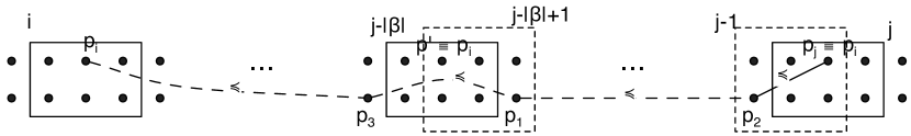
Figure 4: Relations between symbolic valuations $i$ and $j$.

Figure 4 exemplifies the conditions above. We have two cases. If $p^{\prime}\preccurlyeq p_{1}$, then, from conditions 2 and 3, and the definition of $\stackrel{{\scriptstyle\preccurlyeq}}{{\frown}}$, we have $p^{\prime}\stackrel{{\scriptstyle\preccurlyeq}}{{\frown}}p_{j}$; since $p_{i}$, $p^{\prime}$ and $p_{j}$ all belong to $\beta^{\omega}$ and are such that $p_{i}\equiv p^{\prime}\equiv p_{j}$, then the same forward path between $p^{\prime}$ and $p_{j}$ from which it descends $p^{\prime}\stackrel{{\scriptstyle\preccurlyeq}}{{\frown}}p_{j}$ can be iterated starting from $p_{i}$, because suffix $\beta^{\omega}$ is periodic. Then, $p_{i}\stackrel{{\scriptstyle\preccurlyeq}}{{\frown}}p^{\prime}$. If, instead, $p^{\prime}\succcurlyeq p_{1}$, then, by conditions 5 and 6, and definition of $\succcurlyeq$ and $\stackrel{{\scriptstyle\preccurlyeq}}{{\frown}}$, it is also $p_{3}\stackrel{{\scriptstyle\preccurlyeq}}{{\frown}}p^{\prime}$; finally, by condition 4 and transitivity of $\stackrel{{\scriptstyle\preccurlyeq}}{{\frown}}$, we have $p_{i}\stackrel{{\scriptstyle\preccurlyeq}}{{\frown}}p^{\prime}$.

The case $p_{i}\stackrel{{\scriptstyle\prec}}{{\frown}}p_{j}$ is similar, when one considers that, in addition to conditions 1-6, it must be $p_{i}\stackrel{{\scriptstyle\prec}}{{\frown}}p_{3}$, or $p_{3}\stackrel{{\scriptstyle\prec}}{{\frown}}p_{1}$, or $p_{1}\stackrel{{\scriptstyle\prec}}{{\frown}}p_{2}$, or $p_{2}\prec p_{j}$. If $p^{\prime}\preccurlyeq p_{1}$, then if it is $p_{1}\stackrel{{\scriptstyle\prec}}{{\frown}}p_{j}$, it is also $p^{\prime}\stackrel{{\scriptstyle\prec}}{{\frown}}p_{j}$, and the proof is as before. If, instead, it is not $p_{1}\stackrel{{\scriptstyle\prec}}{{\frown}}p_{j}$, then it must be $p^{\prime}\stackrel{{\scriptstyle\prec}}{{\frown}}p_{1}$, otherwise from Remark 1 it descends that the value of the variable in $p^{\prime}$ is equal to the value in $p_{j}$, and in turn that the value of the variable in $p_{i}$ is equal to the value in $p_{j}$, thus contradicting $p_{i}\stackrel{{\scriptstyle\prec}}{{\frown}}p_{j}$. If $p^{\prime}\succcurlyeq p_{1}$, then if $p_{i}\stackrel{{\scriptstyle\prec}}{{\frown}}p_{1}$ we have also $p_{i}\stackrel{{\scriptstyle\prec}}{{\frown}}p^{\prime}$. Otherwise, if it is not $p_{i}\stackrel{{\scriptstyle\prec}}{{\frown}}p_{1}$, then it must be $p_{1}\stackrel{{\scriptstyle\prec}}{{\frown}}p_{j}$, and in this case it must also be $p^{\prime}\succ p_{1}$ (hence also $p_{i}\stackrel{{\scriptstyle\prec}}{{\frown}}p^{\prime}$), or the arc between $p_{1}$ and $p^{\prime}$ is labeled with $=$, and we have that $p_{i}\stackrel{{\scriptstyle\preccurlyeq}}{{\frown}}p^{\prime}$, not $p_{i}\stackrel{{\scriptstyle\prec}}{{\frown}}p^{\prime}$ (hence $p_{i}\stackrel{{\scriptstyle\approx}}{{\frown}}p^{\prime}$ by Remark 1), and $p^{\prime}\stackrel{{\scriptstyle\prec}}{{\frown}}p_{j}$, which yields a contradiction.

The proofs for cases $p_{i}\stackrel{{\scriptstyle\succcurlyeq}}{{\frown}}p_{j}$, $p_{i}\stackrel{{\scriptstyle\succ}}{{\frown}}p_{j}$, and $p_{i}\stackrel{{\scriptstyle\approx}}{{\frown}}p_{j}$ are similar. ∎

We immediately have the following corollary, which states that a path looping through $p_{i}$ can be shortened to a single iteration.

Corollary 3.

Let $\rho=\alpha\beta^{\omega}\in SV(\phi)^{\omega}$, $p_{i}$ and $p_{j}$ as in Lemma 5. Then it is also $p_{i}\stackrel{{\scriptstyle\sim}}{{\frown}}p^{\prime}$, with $p\equiv p^{\prime}$ and $\mathit{sv}(p^{\prime})=i+|\beta|$.

The following lemma shows that there is an infinite non-strict (resp. strict) forward path in $\rho=(\alpha^{\prime}s)(\beta^{\prime}s)^{\omega}$ if, and only if, there is an infinite non-strict (resp. strict) forward path that loops through symbolic valuation $s$.

Lemma 6.

Let $\rho=\alpha\beta^{\omega}\in SV(\phi)^{\omega}$ be an ultimately periodic word, with $\alpha=\alpha^{\prime}s$ and $\beta=\beta^{\prime}s$. In $\rho$ there is an infinite non-strict (resp. strict) forward path if, and only if, there is an infinite non-strict (resp. strict) forward path that contains a denumerable set of points $\{p_{i}\}_{i\in\mathbb{N}}$ of $P_{\rho}$ such that:

1. $\mathit{sv}(p_{0})=|\alpha|-1=|\alpha^{\prime}|$,

2. $p_{i}\equiv p_{j}$ and $\mathit{sv}(p_{i})<\mathit{sv}(p_{j})$ for all $i<j\in\mathbb{N}$,

3. $p_{i}\stackrel{{\scriptstyle\preccurlyeq}}{{\frown}}p_{i+1}$ (resp. $p_{i}\stackrel{{\scriptstyle\prec}}{{\frown}}p_{i+1}$) for all $i\in\mathbb{N}$.

Proof.

Let us assume in $\rho$ there is an infinite non-strict forward path, and let $F=\{f_{i}\}_{i\in\mathbb{N}}$ be the points that it traverses (hence, it is $f_{i}\preccurlyeq f_{i+1}$ for all $i$). Note that $\mathit{sv}(f_{0})$ can be any, not necessarily $0$ or $|\alpha^{\prime}|$. Since suffix $\beta^{\omega}$ is periodic and each arc $\langle f_{i},f_{i+1}\rangle$ in $F$ connects two points that, for Condition 1 of Definition 7, dist at most $-\lfloor\phi\rfloor+\lceil\phi\rceil+1$ from one another, then there must be a sequence of points $Q=\{q_{i}\}_{i\in\mathbb{N}}$ such that, for each $q_{i}\in Q$

• $\mathit{sv}(q_{i+1})>\mathit{sv}(q_{i})>|\alpha^{\prime}|$

• there is a point $f_{j}\in F$ such that $f_{j}$ is locally equivalent to $q_{i}$

• $\rho(\mathit{sv}(q_{i}))=s$.

In other words, $Q$ is made by points of $F$ (or locally equivalent ones) that belong to one of the instances of symbolic valuation $s$ in $\beta^{\omega}$. For each $i\in\mathbb{N}$ it is $q_{i}\stackrel{{\scriptstyle\preccurlyeq}}{{\frown}}q_{i+1}$. Since the number of points in symbolic valuation $s$ is finite, there must be an element $q_{\bar{i}}\in Q$ such that an infinite number of points equivalent to $q_{\bar{i}}$ appear in $Q$. In other words, there is a denumerable sequence $L=\{l_{i}\}_{i\in\mathbb{N}}$ such that

• $l_{0}=q_{\bar{i}}$

• for all $i$ it is $l_{i}\equiv q_{\bar{i}}$.

Again, for all $i$ it is $l_{i}\stackrel{{\scriptstyle\preccurlyeq}}{{\frown}}l_{i+1}$ (also, it is $\mathit{sv}(l_{i})<\mathit{sv}(l_{i+1})$). Sequence $L$ is part of an infinite forward path that starts from $l_{0}$ and visits all $l_{i}$. The desired sequence $\{p_{i}\}_{i\in\mathbb{N}}$ that satisfies conditions 1-3 is $L$ translated of $\mathit{sv}(l_{0})-|\alpha^{\prime}|$, so that it starts from symbolic valuation in position $|\alpha^{\prime}|$ (the translation is possible because of the periodicity of $\beta^{\omega}$). Figure 5 shows an example of translation.

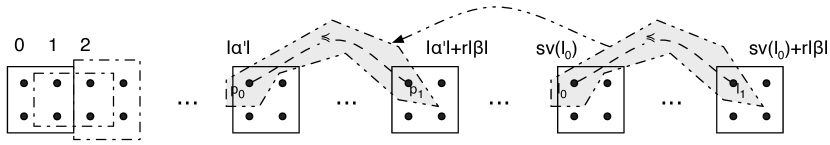
Figure 5: Example of translation from $l_{0}$ to $p_{0}$.

The proof in case of strict infinite paths is similar. ∎

A similar lemma holds for backward paths. We have the following result.

Theorem 4.

Let $\rho=\alpha\beta^{\omega}\in SV(\phi)^{\omega}$ be an ultimately periodic word, with $\alpha=\alpha^{\prime}s$ and $\beta=\beta^{\prime}s$. Then, there is a non-strict (resp. strict) infinite forward path in $\rho$ if, and only if, there are two points $p,p^{\prime}$ of $P_{\rho}$ such that $\mathit{sv}(p)=|\alpha^{\prime}|$, $\mathit{sv}(p^{\prime})=k$, $p\equiv p^{\prime}$, and $p\stackrel{{\scriptstyle\preccurlyeq}}{{\frown}}p^{\prime}$ (resp. $p\stackrel{{\scriptstyle\prec}}{{\frown}}p^{\prime}$).

Proof.

We consider the case for non-strict forward paths, the case for strict ones being similar.

Assume in $\rho$ there is an infinite non-strict forward path; then, by Lemma 6 there is also an infinite non-strict forward path that contains a denumerable set of points $\{p_{i}\}_{i\in\mathbb{N}}$ that satisfies conditions 1-3 of the lemma. Then, from Corollary 3 we immediately have $p_{0}\stackrel{{\scriptstyle\preccurlyeq}}{{\frown}}p^{\prime}$, with $p^{\prime}\equiv p_{0}$ and $\mathit{sv}(p^{\prime})=|\alpha^{\prime}|+|\beta|=k$ (recall that $|\alpha\beta|=k+1$).

Conversely, assume that there are two points $p,p^{\prime}$ such that $p=(x,|\alpha^{\prime}|,h)$, $p^{\prime}=(x,k,h)$, $p\equiv p^{\prime}$, and $p\stackrel{{\scriptstyle\preccurlyeq}}{{\frown}}p^{\prime}$. By definition of $p\stackrel{{\scriptstyle\preccurlyeq}}{{\frown}}p^{\prime}$, there exists a finite number of points $p^{1},p^{2},\dots$ such that $p\preccurlyeq p^{1}\preccurlyeq p^{2}\dots\preccurlyeq p^{\prime}$. This forward path can be iterated infinitely many times, since $p\equiv p^{\prime}$ and the suffix $\beta$ is repeated infinitely often. Therefore, point $p$ and points equivalent to $p$ satisfy conditions 1-3 of Lemma 6. By the same lemma, then, in $\rho$ there is an infinite non-strict forward path. ∎

Analogously, we can prove the following version of Theorem 4 in case of backward paths.

Theorem 5.

Let $\rho=\alpha\beta^{\omega}\in SV(\phi)^{\omega}$ be an ultimately periodic word, with $\alpha=\alpha^{\prime}s$ and $\beta=\beta^{\prime}s$. Then, there is a non-strict (resp. strict) infinite backward path in $\rho$ if, and only if, there are two points $p,p^{\prime}$ such that $\mathit{sv}(p)=|\alpha^{\prime}|$, $\mathit{sv}(p^{\prime})=k$, $p\equiv p^{\prime}$, and $p\stackrel{{\scriptstyle\succcurlyeq}}{{\frown}}p^{\prime}$ (resp. $p\stackrel{{\scriptstyle\succ}}{{\frown}}p^{\prime}$).

Our condition for the non existence of an arithmetic model for symbolic model $\rho=\alpha^{\prime}s(\beta^{\prime}s)^{\omega}$ (with $|\alpha^{\prime}s\beta^{\prime}s|=k+1$) if formalized by Formula (1) below; it captures Property 1 and takes advantage of the previous Theorems 4 and 5.

$$\begin{gathered}\exists p_{1}p_{2}p_{1}^{\prime}p_{2}^{\prime}\left(\begin{gathered}p_{1}\equiv p_{2}\ \wedge\ p_{1}^{\prime}\equiv p^{\prime}_{2}\ \wedge\\ \mathit{sv}(p_{1})=\mathit{sv}(p^{\prime}_{1})=|\alpha^{\prime}|\ \wedge\ \mathit{sv}(p_{2})=\mathit{sv}(p^{\prime}_{2})=k\ \wedge\\ p_{1}\stackrel{{\scriptstyle\preccurlyeq}}{{\frown}}p_{2}\ \wedge\ \ p^{\prime}_{1}\stackrel{{\scriptstyle\succcurlyeq}}{{\frown}}p^{\prime}_{2}\ \wedge\ (p_{1}\stackrel{{\scriptstyle\prec}}{{\frown}}p_{2}\ \vee\ \ p^{\prime}_{1}\stackrel{{\scriptstyle\succ}}{{\frown}}p^{\prime}_{2})\ \wedge\\ \ (p_{1}\prec p_{1}^{\prime}\vee{p_{1}^{\prime}}\succ{p_{1}})\end{gathered}\right).\end{gathered}$$ (1)

In Formula (1) four conditions are defined, similar to those of Property 1. Informally, Formula (1) says that:

1. there is an infinite forward path $f$ from $p_{1}$ (this derives from the fact that $p_{1}\stackrel{{\scriptstyle\preccurlyeq}}{{\frown}}p_{2}$, with $p_{1}\equiv p_{2}$, $\mathit{sv}(p_{1})=|\alpha^{\prime}|$, and $\mathit{sv}(p_{2})=k$);

2. there is an infinite backward path $b$ from $p_{1}^{\prime}$ (from $p_{1}^{\prime}\stackrel{{\scriptstyle\succcurlyeq}}{{\frown}}p_{2}^{\prime}$, with $p_{1}^{\prime}\equiv p_{2}^{\prime}$, where $\mathit{sv}(p_{1}^{\prime})=|\alpha^{\prime}|$, and $\mathit{sv}(p_{2}^{\prime})=k$);

3. at least one between $f$ and $b$ is strict;

4. between $p_{1}$ and $p_{1}^{\prime}$ there is an edge labeled with $<$.

In particular, condition $4$ of Property 1 is different from condition $4$ of Formula (1). In fact, the former one states that for each $i,j\in\mathbb{N}$, given a forward path $d$ and a backward path $e$, whenever $d(i)$ and $e(j)$ belong to the same symbolic valuation (i.e., $|i-j|<-\lfloor\phi\rfloor+\lceil\phi\rceil+1$) there is an edge labeled by $<$ from $d(i)$ to $e(j)$. In other words, this means that point $p_{d}$ representing $d(i)$ and point $p_{e}$ representing $e(j)$ are such that either $p_{d}\prec p_{e}$ or $p_{e}\succ p_{d}$. The next theorem shows that the conditions are nevertheless equivalent when $\rho=\alpha\beta^{\omega}$. In fact, whereas Property 1 is defined for a general $G_{\rho}$, Formula (1) is tailored to the finite representation of ultimately periodic symbolic models $\rho=\alpha\beta^{\omega}$.

Theorem 6.

Over ultimately periodic symbolic models of the form $\alpha^{\prime}s(\beta^{\prime}s)^{\omega}$, with $\alpha,\beta\in SV(\phi)^{*}$ and $s\in SV(\phi)$, Property 1 is equivalent to Formula (1).

Proof.

Let $\rho=\alpha^{\prime}s(\beta^{\prime}s)^{\omega}$ be an infinite symbolic model and assume that Formula (1) holds in $\alpha^{\prime}s\beta^{\prime}s$. Therefore, by Theorems 4 and 5, there exists a pair of points $p_{1}$ and $p_{1}^{\prime}$, such that $\mathit{sv}(p_{1})=\mathit{sv}(p_{1}^{\prime})=|\alpha^{\prime}|$, visited respectively by an infinite forward path and an infinite backward path, where at least one of the two is strict (because $p_{1}\stackrel{{\scriptstyle\prec}}{{\frown}}p_{2}\vee p^{\prime}_{1}\stackrel{{\scriptstyle\succ}}{{\frown}}p^{\prime}_{2}$ holds). Since $p_{1}\prec p_{1}^{\prime}\vee p_{1}^{\prime}\succ p_{1}$ holds, and $\equiv$ is a congruence for $\prec,\succ$, then also $p_{2}\prec p_{2}^{\prime}$ or $p_{2}^{\prime}\succ p_{2}$ hold. Now, consider any two points $u$ and $v$ in $\alpha^{\prime}s\beta^{\prime}s$, such that $\mathit{sv}(u)=\mathit{sv}(v)$ and $u$ (resp. $v$) belongs to the infinite strict forward (resp. backward) path from $p_{1}$ (resp. $p_{1}^{\prime}$). Then, it is $u\stackrel{{\scriptstyle\preccurlyeq}}{{\frown}}p_{2}$, $v\stackrel{{\scriptstyle\succcurlyeq}}{{\frown}}p_{2}^{\prime}$, and $p_{2}\prec p_{2}^{\prime}$ or $p_{2}^{\prime}\succ p_{2}$. Hence, it is also $u\prec v$ or $v\succ u$, i.e., between $u$ and $v$ there is an edge labeled with $<$.

Conversely, assume Property 1 holds; then, by Theorems 4 and 5 there are points $p_{1},p_{1}^{\prime},p_{2},p_{2}^{\prime}$ such that $\mathit{sv}(p_{1})=\mathit{sv}(p_{1}^{\prime})=|\alpha^{\prime}|$, $\mathit{sv}(p_{2})=\mathit{sv}(p_{2}^{\prime})=k$, $p_{1}\equiv p_{2}$, $p_{1}^{\prime}\equiv p_{2}^{\prime}$, $p_{1}\stackrel{{\scriptstyle\preccurlyeq}}{{\frown}}p_{2}$, $p_{1}^{\prime}\stackrel{{\scriptstyle\succcurlyeq}}{{\frown}}p_{2}^{\prime}$, and $p_{1}\stackrel{{\scriptstyle\preccurlyeq}}{{\frown}}p_{2}\vee p_{1}^{\prime}\stackrel{{\scriptstyle\succcurlyeq}}{{\frown}}p_{2}^{\prime}$ hold. From the proof of Theorem 4, point $p_{1}$ is equivalent to some point in the original forward path; similarly for point $p_{1}^{\prime}$. Then, since $p_{1}$ and $p_{1}^{\prime}$ belong to the same symbolic valuation, by condition 4 of Property 1, they are connected through an edge labeled with $<$, i.e., $p_{1}\prec p_{1}^{\prime}$ or $p_{1}^{\prime}\succ p_{1}$ hold. ∎

The next theorem extends Proposition 5 to constraint system IPC^∗, which does not benefit from the completion property.

Proposition 6.

Let $\phi\in$ CLTLB$(\mathcal{D})$ and $\mathcal{D}$ be IPC^∗. Formula $\phi$ is $k$-satisfiable and Formula (1) does not hold if, and only if, thre exists a model $\sigma$ such that $\sigma,0\models\phi$.

Proof.

By Theorems 1, 2, and 3, $\phi$ is $k$-satisfiable if, and only if, formula $|\phi|_{k}$ is satisfiable; in addition, when formula $|\phi|_{k}$ is satisfiable, it induces a model $\sigma_{k}$ and a sequence $\alpha\beta$ of symbolic valuations of length $k$ representing an infinite sequence $\rho=\alpha\beta^{\omega}$ of symbolic valuations such that $\rho\,|\!\!\!\ext@arrow 0359\arrowfill@\Relbar\Relbar\Relbar{}{\mbox{\it{\tiny sym}}}\phi$. Since Formula (1) does not hold, then by Theorem 6 Property 1 does not hold, hence, by Lemma 2, $\rho$ admits a model $\sigma$ such that $\sigma,0\models\phi$.

Conversely, if formula $\phi$ is satisfiable, then automaton $\mathcal{A}_{\phi}$ recognizes models which satisfy condition $C$. Then, a symbolic model $\alpha\beta^{\omega}\in\mathscr{L}(\mathcal{A}_{\phi})$ and a model $\sigma_{k},0\models_{k}\alpha\beta$ can be obtained as in the proof of Proposition 5. ∎

Bounded Encoding of Formula (1)

The encoding shown afterwards represents, by means of a finite representation, infinite – strict and non strict – paths over infinite symbolic models. As before, we consider models $\rho=\alpha\beta^{\omega}$ where $\alpha=\alpha^{\prime}s$ and $\beta=\beta^{\prime}s$, and we consider the finite sequence of symbolic valuations $\alpha^{\prime}s\beta^{\prime}s$, of length $k+1$. We indicate by $P_{\alpha\beta}\subset P_{\rho}$ the set of points of finite path $\alpha^{\prime}s\beta^{\prime}s$ (for all $p\in P_{\alpha\beta}$, it is $\mathit{sv}(p)\in[0,k]$). We use the points of $P_{\alpha\beta}$ to capture properties of $P_{\rho}$. To encode the previous formulae into QF-EU$\mathcal{D}$ formulae, where $\mathcal{D}$ is a suitable constraint system embedding $\mathbb{N}$ and having the successor function plus order $<$, we rearrange the formulae above by splitting information, which is now encapsulated in the notion of point, on variables and positions over the model. Predicate $\bm{f}^{<}_{x,y}:\mathbb{N}^{3}\rightarrow\{true,false\}$ for all pairs $x,y\in V\cup\mathit{const}(\phi)$ (resp. $\bm{f}^{\leq}_{x,y}$) encodes relation $p_{1}\prec p_{2}$ (resp. $p_{1}\preccurlyeq p_{2}$) where $p_{1}=(x,j,h)$ and $p_{2}=(y,j,m)$.

$$\begin{array}[]{c|c}0\leq j\leq k\text{ and }h\leq m&0\leq j\leq k\text{ and }h>m\\ \hline\cr\bm{f}^{<}_{x,y}(j,h,m)\Leftrightarrow\sigma_{k}(j+h,x)<\sigma_{k}(j+m,y)&\neg\bm{f}^{<}_{x,y}(j,h,m)\\ \bm{f}^{\leq}_{x,y}(j,h,m)\Leftrightarrow\sigma_{k}(j+h,x)\leq\sigma_{k}(j+m,y)&\neg\bm{f}^{\leq}_{x,y}(j,h,m)\end{array}$$

for all $h,m\in[\lfloor\phi\rfloor,\lceil\phi\rceil]$. The value of $\sigma_{k}(0+h,x)$ equals the value of term $\alpha=\mathrm{Y}^{|h|}x$, for $h\in[\lfloor\phi\rfloor,-1]$, or of term $\alpha=\mathrm{X}^{h}x$, for $h\in[0,\lceil\phi\rceil]$. For example, $\sigma_{k}(0+h,x)$ is $\bm{\alpha}(0)$, and $\sigma_{k}(k+h,x)$ is $\bm{\alpha}(k)$ (see $|ArithConstraints|_{k}$ in Section 3.3). Constants are implicitly included in the model. For instance, if $5\in\mathit{const}(\phi)$ and $x\in V$ we have the following formulae $\bm{f}^{<}_{x,5}(j,h,m)\text{ iff }\sigma_{k}(j+h,x)<5$ and $\bm{f}^{<}_{5,x}(j,h,m)\text{ iff }5<\sigma_{k}(j+m,x)$. When $x,y\in\mathit{const}(\phi)$ then $\bm{f}^{<}_{x,y}\text{ iff }x<y$ and $\bm{f}^{\leq}_{x,y}\text{ iff }x\leq y$ for all $0\leq j\leq k$ and $h\leq m$; $\neg\bm{f}^{<}_{x,y}$ and $\neg\bm{f}^{<}_{x,y}$ for all $0\leq j\leq k$ and $h>m$.

Relation $\stackrel{{\scriptstyle\prec}}{{\frown}}$ (resp. $\stackrel{{\scriptstyle\preccurlyeq}}{{\frown}}$) is encoded by uninterpreted predicates $\bm{F}^{<}_{x,y}:\mathbb{N}^{4}\rightarrow\{true,false\}$ (resp. $\bm{F}^{\leq}_{x,y}:\mathbb{N}^{4}\rightarrow\{true,false\}$) for all pairs of variables $x,y\in V\cup\mathit{const}(\phi)$. To build in practice $\stackrel{{\scriptstyle\prec}}{{\frown}}$ (resp., $\stackrel{{\scriptstyle\preccurlyeq}}{{\frown}}$) through $\bm{F}^{<}$ (resp. $\bm{F}^{\leq}$), over points of the symbolic model $\alpha^{\prime}s\beta^{\prime}s$, we construct the transitive closure of $\bm{F}^{<}$ (resp. $\bm{F}^{\leq}$) explicitly. Starting from $\rho(0)$, we propagate the information about relations $\prec$ and $\preccurlyeq$ that are represented by $\bm{f}^{<}$ and $\bm{f}^{\leq}$ among all points representing variables of model $\rho$. In fact, it is immediate to show that $p_{1}\stackrel{{\scriptstyle\prec}}{{\frown}}p_{2}$ holds if, and only if, there is a point $p$ such that either $p_{1}\prec p$ and $p\stackrel{{\scriptstyle\preccurlyeq}}{{\frown}}p_{2}$ or $p_{1}\preccurlyeq p$ and $p\stackrel{{\scriptstyle\prec}}{{\frown}}p_{2}$ (note that $p$ cannot be locally equivalent to both $p_{1}$ and $p_{2}$, but it can be locally equivalent to one of them). Similarly for the other relations. Figure 6 provides a graphical representation for $\stackrel{{\scriptstyle\prec}}{{\frown}}$.

Figure 6: Adjacent symbolic valuations $\rho(i)$ (solid line) and $\rho(i+1)$ (dotted line) not covering both points $p_{1}=(y,i,-1)$ and $p_{2}=(x,j,h)$ (with $j>i$ and $-1\leq h\leq 1$) of the model, with $p_{1}\prec p$, $p\stackrel{{\scriptstyle\preccurlyeq}}{{\frown}}p_{2}$ and $p_{1}\stackrel{{\scriptstyle\prec}}{{\frown}}p_{2}$.

Formulae defining $\bm{F}^{<}_{x,y}$ and $\bm{F}^{\leq}_{x,y}$ are the following:

$$\bm{F}^{<}_{x,y}(j,h,i,m) \Leftrightarrow\left\{\begin{gathered}\bigvee_{z\in V}\bigvee_{u=\lfloor\phi\rfloor}^{\lceil\phi\rceil}\bm{f}^{<}_{x,z}(j,h,u)\wedge\bm{F}^{\leq}_{z,y}(j,u,i,m)\vee\\ \bigvee_{z\in V}\bigvee_{u=\lfloor\phi\rfloor}^{\lceil\phi\rceil}\bm{f}^{\leq}_{x,z}(j,h,u)\wedge\bm{F}^{<}_{z,y}(j,u,i,m)\end{gathered}\right.$$ (4)

$$\bm{F}^{\leq}_{x,y}(j,h,i,m) \Leftrightarrow\bigvee_{z\in V}\bigvee_{u=\lfloor\phi\rfloor}^{\lceil\phi\rceil}\bm{f}^{\leq}_{x,z}(j,h,u)\wedge\bm{F}^{\leq}_{z,y}(j,u,i,m)$$ (5)

for all $j,i\in[0,k]$ with $j<i$ and for all $h,m\in[\lfloor\phi\rfloor,\lceil\phi\rceil]$ such that $i+m-(j+h)>-\lfloor\phi\rfloor+\lceil\phi\rceil$, $h=\lfloor\phi\rfloor$, $(x=z)\Rightarrow(h\neq u)$ and for all pairs $x,y\in V\cup\mathit{const}(\phi)$. When $j=i\in[0,k]$ and $h\leq m$, with $h,m\in[\lfloor\phi\rfloor,\lceil\phi\rceil]$:

$$\bm{F}^{<}_{x,y}(j,h,j,m) \Leftrightarrow\bm{f}^{<}_{x,y}(j,h,m)$$

$$\bm{F}^{\leq}_{x,y}(j,h,j,m) \Leftrightarrow\bm{f}^{\leq}_{x,y}(j,h,m)$$

When $j+h>i+m$:

$$\neg\bm{F}^{<}_{x,y}(j,h,i,m)$$

$$\neg\bm{F}^{\leq}_{x,y}(j,h,i,m)$$

Figure 7 shows how predicate $\bm{F}^{<}_{x,x}(i,0,j,1)$ is defined as conjunction of local relation $\bm{f}^{<}_{x,y}(i,0,1)$ and of $\bm{F}^{\leq}_{y,x}(i,1,j,1)$.

Figure 7: Definition of $\bm{F}^{<}$ by local relations $\bm{f}^{<}$.

The following formula $|CongruenceConstraints|_{k}$ defines congruence classes of locally equivalent points for relations $\stackrel{{\scriptstyle\prec}}{{\frown}},\stackrel{{\scriptstyle\preccurlyeq}}{{\frown}}$ captured by predicates $\bm{F}^{<}$ and $\bm{F}^{\leq}$. In fact, observe that, since from $p_{1}\preccurlyeq p_{2}$ we obtain $p^{\prime}_{1}\preccurlyeq p^{\prime}_{2}$, for all $p_{1}^{\prime}$ (resp. $p_{2}^{\prime}$) that is locally equivalent to $p_{1}$ (resp. $p_{2}^{\prime}$), then, in general, the congruence extends to $\stackrel{{\scriptstyle\preccurlyeq}}{{\frown}}$; i.e., from $p_{1}\stackrel{{\scriptstyle\preccurlyeq}}{{\frown}}p_{2}$ we obtain $p^{\prime}_{1}\stackrel{{\scriptstyle\preccurlyeq}}{{\frown}}p^{\prime}_{2}$ for all $p_{1}^{\prime},p_{2}^{\prime}$ locally equivalent to $p_{1},p_{2}$. An analogous argument holds for $\stackrel{{\scriptstyle\prec}}{{\frown}}$, $\stackrel{{\scriptstyle\succcurlyeq}}{{\frown}}$ and $\stackrel{{\scriptstyle\succ}}{{\frown}}$.

$$\begin{array}[]{c|c|c}i\in[1,k]&m\in[\lfloor\phi\rfloor,\lceil\phi\rceil]&j\\ \hline\cr\bm{F}^{<}_{x,y}(j,h,i,m)\Leftrightarrow\bm{F}^{<}_{x,y}(j+1,h-1,i,m)&h\in[\lfloor\phi\rfloor+1,\lceil\phi\rceil]&[0,i-1]\\ \bm{F}^{<}_{x,y}(j,h,i,m)\Leftrightarrow\bm{F}^{<}_{x,y}(j-1,h+1,i,m)&h\in[\lfloor\phi\rfloor,\lceil\phi\rceil-1]&[1,i]\end{array}$$

$$\begin{array}[]{c|c|c}j\in[0,k-1]&h\in[\lfloor\phi\rfloor,\lceil\phi\rceil]&i\\ \hline\cr\bm{F}^{<}_{x,y}(j,h,i,m)\Leftrightarrow\bm{F}^{<}_{x,y}(j,h,i+1,m-1)&m\in[\lfloor\phi\rfloor+1,\lceil\phi\rceil]&i\in[j,k-1]\\ \bm{F}^{<}_{x,y}(j,h,i,m)\Leftrightarrow\bm{F}^{<}_{x,y}(j,h,i-1,m+1)&m\in[\lfloor\phi\rfloor,\lceil\phi\rceil-1]&i\in[j+1,k].\end{array}$$

Predicates $\bm{b}^{>}_{x,y},\bm{b}^{\geq}_{x,y}$ for local backward paths $\succ,\succcurlyeq$, predicates $\bm{B}^{>}_{x,y},\bm{B}^{\geq}_{x,y}$ for backward paths $\stackrel{{\scriptstyle\succ}}{{\frown}},\stackrel{{\scriptstyle\succcurlyeq}}{{\frown}}$ and congruence among points are defined similarly. For brevity, we only show the definition of $\bm{b}^{>}_{x,y}$ and $\bm{b}^{\geq}_{x,y}$, the others are straightforward.

$$\begin{array}[]{c|c}0\leq j\leq k\text{ and }h\leq m&0\leq j\leq k\text{ and }h>m\\ \hline\cr\bm{b}^{>}_{x,y}(j,h,m)\Leftrightarrow\sigma_{k}(j+h,x)>\sigma_{k}(j+m,y)&\neg\bm{b}^{>}_{x,y}(j,h,m)\\ \bm{b}^{\geq}_{x,y}(j,h,m)\Leftrightarrow\sigma_{k}(j+h,x)\geq\sigma_{k}(j+m,y)&\neg\bm{b}^{\geq}_{x,y}(j,h,m)\end{array}$$

for all $h,m\in[\lfloor\phi\rfloor,\lceil\phi\rceil]$. When both $x,y\in const(\phi)$ then $\bm{b}^{>}_{x,y}(j,h,m)\text{ iff }x>y$ and $\bm{b}^{\geq}_{x,y}(j,h,m)\text{ iff }x\geq y$ for all $0\leq j\leq k$ and $h\leq m$; $\neg\bm{b}^{>}_{x,y}(j,h,m)$ and $\neg\bm{b}^{\geq}_{x,y}(j,h,m)$ for all $0\leq j\leq k$ and $h>m$.

Finally, the condition of existence defined by Formula (1) is encoded by the following QF-EU$\mathcal{D}$ formula. The condition is parametric with respect to a pair of variables $x,x^{\prime}\in V\cup\mathit{const}(\phi)$. The condition is meaningful only if $x\neq x^{\prime}$ and if either $x\notin\mathit{const}(\phi)$ or $x^{\prime}\notin\mathit{const}(\phi)$. In fact, a constant value never generates a strict (forward or backward) path; therefore, two constants can not satisfy the condition of non-existence of an arithmetical model. Formula $C_{x,x^{\prime}}$ below captures the existence in $\rho(|\alpha^{\prime}|)$ of a strict relation $<$ between two points, one of a forward and one of backward path, which involve variables $x$ and $x^{\prime}$. Variable $\bm{loop}$ has already been introduced in Section 7 and defines the position where, in $\alpha\beta$, suffix $\beta$ starts (as already explained $|\alpha^{\prime}|=\bm{loop}-1$).

$$C_{x,x^{\prime}}:=\bigvee_{h,h^{\prime}\in[\lfloor\phi\rfloor,\lceil\phi\rceil]}\left(\begin{gathered}\left(\begin{gathered}\bm{F}^{\leq}_{x,x}(\bm{loop}-1,h,k,h)\wedge\bm{B}^{>}_{x^{\prime},x^{\prime}}(\bm{loop}-1,h^{\prime},k,h^{\prime})\\ \vee\\ \bm{F}^{<}_{x,x}(\bm{loop}-1,h,k,h)\wedge\bm{B}^{\geq}_{x^{\prime},x^{\prime}}(\bm{loop}-1,h^{\prime},k,h^{\prime})\end{gathered}\right)\\ \wedge\\ \bm{f}^{<}_{x,x^{\prime}}(\bm{loop}-1,h,h^{\prime})\vee\bm{b}^{>}_{x^{\prime},x}(\bm{loop}-1,h^{\prime},h)\\ \end{gathered}\right).$$

In Formula $C_{x,x^{\prime}}$, we use explicitly points that were symbolically represented in Formula (1): $p_{1}=(x,loop-1,h)$, $p^{\prime}_{1}=(x^{\prime},loop-1,h^{\prime})$, $p_{2}=(x,k,h)$, $p^{\prime}_{2}=(x^{\prime},k,h^{\prime})$. It is immediate to see that formula $\bm{f}^{<}_{x,x^{\prime}}(\bm{loop}-1,h,h^{\prime})\vee\bm{b}^{>}_{x^{\prime},x}(\bm{loop}-1,h^{\prime},h)$ encodes $p_{1}\prec p_{1}^{\prime}\vee p_{1}^{\prime}\succ p_{1}$ of Formula (1) and formula $\bm{F}^{\leq}_{x,x}(\bm{loop}-1,h,k,h)\wedge\bm{B}^{>}_{x^{\prime},x^{\prime}}(\bm{loop}-1,h^{\prime},k,h^{\prime})$ , encodes $p_{1}\stackrel{{\scriptstyle\preccurlyeq}}{{\frown}}p_{2}\wedge p_{1}^{\prime}\stackrel{{\scriptstyle\preccurlyeq}}{{\frown}}p_{2}^{\prime}\wedge p_{1}\stackrel{{\scriptstyle\prec}}{{\frown}}p_{2}$ (similarly for formula $\bm{F}^{<}_{x,x}(\bm{loop}-1,h,k,h)\wedge\bm{B}^{\geq}_{x^{\prime},x^{\prime}}(\bm{loop}-1,h^{\prime},k,h^{\prime})$).

The existence condition of an arithmetical model is captured by the formula:

$$\bigwedge_{\footnotesize\begin{array}[]{c}x,x^{\prime}\in V\cup\mathit{const}(\phi)\\ x\neq x^{\prime},x\notin\mathit{const}(\phi)\lor x^{\prime}\notin\mathit{const}(\phi)\end{array}}\neg C_{x,x^{\prime}}$$ (6)

Given a CLTLB$(\textrm{IPC}^{*})$ formula $\phi$, the satisfiability of $\phi$ is reduced to the satisfiability of the following QF-EU($\mathcal{D}$) formula:

$$|\phi|_{k}\land\eqref{qf-euf-condition-C}.$$ (7)

If Formula (7) is unsatisfiable, then either $\phi$ does not admit symbolic models, or none of its symbolic models admits arithmetic models. Conversely, if Formula (7) is satisfiable, then there is a symbolic model $\rho$ of $\phi$ for which condition (6) holds, hence $\rho$ admits an arithmetic model and $\phi$ is satisfiable.

4.1 Simplifying the condition of existence of arithmetical models

In this section, we relax the condition of existence of an arithmetical model $\sigma$ for sequences of symbolic valuations of CLTLB(IPC^∗) formulae. In fact, Property 1 is stronger than necessary in those cases in which not all variables appearing in a formula $\phi$ are compared against each other. Consider for example the following formula

$$\mathbf{G}(x<\mathrm{X}x\wedge\neg(y<\mathrm{X}y))$$ (8)

which enforces strict increasing monotonicity for variable $x$ and decreasing monotonicity for variable $y$. Figure 8 shows a symbolic model for Formula (8) which does not admit arithmetic model, as it does not satisfy Property 1 (in fact, the strict forward path that visits all points $\{(x,i,0)\}_{i\in\mathbb{N}}$ and the strict backward path that visits all points $\{(y,i,0)\}_{i\in\mathbb{N}}$ are such that, for all $i$, $(x,i,0)\prec(y,i,0)$).

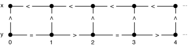
Figure 8: A symbolic model for Formula (8) that does not admit an arithmetical model.

However, in Formula (8) $x$ and $y$ are not compared, neither directly, nor indirectly, so if we disregard the relations between them in the symbolic model of Figure 8, and produce an assignment of the variables that only respects the relations between variables that are actually compared in the formula (i.e., $x$ with itself, and $y$ with itself) we obtain an arithmetic model for Formula (8). Figure 9 shows a “weaker” version of the symbolic model of Figure 8, one that is more concise to encode into QF-EU($\mathcal{D}$) formulae than the maximally consistent one, as it does not contain any comparison between unrelated terms.

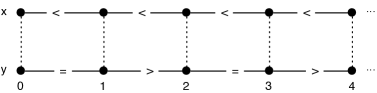
Figure 9: A weak symbolic model for Formula (8).

To characterize sequences of symbolic valuations which do not take into account relations among variables that are not compared with each other in a formula $\phi$, we first remark that $\phi$ induces a finite partition $\{V_{1},\dots,V_{h}\}$ of set $V$ such that $x,y\in V_{i}$ if and only if there is an IPC^∗ constraint $R(\mathrm{X}^{i}x,\mathrm{X}^{j}y)$ occurring in $\phi$, for some $i,j\in\mathbb{Z}$ (where we write $\mathrm{X}^{-n}$, with $n>0$, instead of $\mathrm{Y}^{n}$). Then, we introduce the notions of weak symbolic valuation and of sequence of weak symbolic valuations.

Definition 11.

Given a symbolic valuation $sv\in SV(\phi)$, its weak version $\overline{sv}$ is obtained by removing from $sv$ all relations $R(\mathrm{X}^{i}x,\mathrm{X}^{j}y)$ where $x\in V_{l}$ and $y\in V_{t}$ with $l\neq t$. We similarly define the weak version $\overline{\rho}$ of a sequence $\rho$ of symbolic valuations.

Given a CLTLB(IPC^∗) formula $\phi$, we indicate with $SV_{w}(\phi)$ the set of all its weak symbolic valuations. A weak symbolic model $\overline{\rho}\in SV_{w}(\phi)^{\omega}$ of $\phi$ is a sequence of weak symbolic valuations such that $\overline{\rho},0\,|\!\!\!\ext@arrow 0359\arrowfill@\Relbar\Relbar\Relbar{}{\mbox{\it{\tiny sym}}}\phi$. Given $\rho\in SV(\phi)^{\omega}$ and its weak version $\overline{\rho}$, $G_{\overline{\rho}}$ is the subgraph of $G_{\rho}$ ontained by removing all arcs between points $p=(x,j,h)$, $p^{\prime}=(y,i,m)$ such that $x\in V_{l}$, $y\in V_{t}$, and $l\neq t$.

The next lemma shows that focusing on weak symbolic valuations is enough to determine whether symbolic models for $\phi$ exist or not.

Lemma 7.

Let $\phi$ be a CLTLB(IPC^∗) formula. Given $\rho\in SV(\phi)^{\omega}$ such that $\rho,0\,|\!\!\!\ext@arrow 0359\arrowfill@\Relbar\Relbar\Relbar{}{\mbox{\it{\tiny sym}}}\phi$, it is also $\overline{\rho},0\,|\!\!\!\ext@arrow 0359\arrowfill@\Relbar\Relbar\Relbar{}{\mbox{\it{\tiny sym}}}\phi$. Conversely, given a sequence $\nu\in SV_{w}(\phi)$ of weak symbolic valuations, if $\nu,0\,|\!\!\!\ext@arrow 0359\arrowfill@\Relbar\Relbar\Relbar{}{\mbox{\it{\tiny sym}}}\phi$, then for any $\rho\in SV(\phi)$ such that $\overline{\rho}=\nu$ it is also $\rho,0\,|\!\!\!\ext@arrow 0359\arrowfill@\Relbar\Relbar\Relbar{}{\mbox{\it{\tiny sym}}}\phi$.

Proof.

Assume that $\rho\,|\!\!\!\ext@arrow 0359\arrowfill@\Relbar\Relbar\Relbar{}{\mbox{\it{\tiny sym}}}\phi$. We only need to focus on the base case, as the inductive one is trivial. For all $i$ and $R(\alpha_{1},\alpha_{2})$ occurring in $\phi$, $\rho,i\,|\!\!\!\ext@arrow 0359\arrowfill@\Relbar\Relbar\Relbar{}{\mbox{\it{\tiny sym}}}R(\alpha_{1},\alpha_{2})$ if, and only if, $R(\alpha_{1},\alpha_{2})\in\rho(i)$. Since $R(\alpha_{1},\alpha_{2})$ occurs in $\phi$ then, by Definition 11, it is also $R(\alpha_{1},\alpha_{2})\in\overline{\rho}(i)$, hence $\overline{\rho},i\,|\!\!\!\ext@arrow 0359\arrowfill@\Relbar\Relbar\Relbar{}{\mbox{\it{\tiny sym}}}R(\alpha_{1},\alpha_{2})$.

The converse case is similar. If $\nu\in SV_{w}(\phi)$ is such that $\nu,0\,|\!\!\!\ext@arrow 0359\arrowfill@\Relbar\Relbar\Relbar{}{\mbox{\it{\tiny sym}}}\phi$, then for all $i$ and $R(\alpha_{1},\alpha_{2})$ that occurs in $\phi$ it is $\nu,i\,|\!\!\!\ext@arrow 0359\arrowfill@\Relbar\Relbar\Relbar{}{\mbox{\it{\tiny sym}}}R(\alpha_{1},\alpha_{2})$ if, and only if, $R(\alpha_{1},\alpha_{2})\in\nu(i)$; in addition, for any $\rho$ such that $\overline{\rho}=\nu$ we have $R(\alpha_{1},\alpha_{2})\in\rho(i)$ if, and only if, $R(\alpha_{1},\alpha_{2})\in\nu(i)$. Finally, $\nu,i\,|\!\!\!\ext@arrow 0359\arrowfill@\Relbar\Relbar\Relbar{}{\mbox{\it{\tiny sym}}}R(\alpha_{1},\alpha_{2})$ implies $\rho,i\,|\!\!\!\ext@arrow 0359\arrowfill@\Relbar\Relbar\Relbar{}{\mbox{\it{\tiny sym}}}R(\alpha_{1},\alpha_{2})$. ∎

We have the following variant of Lemma 2, which defines a condition of existence of arithmetical models for symbolic ones that is checked on their weak countersparts.

Lemma 8.

Let $\phi$ be a CLTLB(IPC^∗) formula. Given an ultimately periodic, locally consistent sequence $\rho\in SV(\phi)^{\omega}$ of symbolic valuations, if there is $\sigma:\mathbb{Z}\times V\to D$ such that $\sigma,0\models\rho$, then Property 1 holds for graph $G_{\overline{\rho}}$. Conversely, if $\nu\in SV_{w}(\phi)^{\omega}$ is an ultimately periodic, locally consistent sequence of weak symbolic valuations such that Property 1 holds for graph $G_{\nu}$, then there are $\sigma$, $\rho$ such that $\overline{\rho}=\nu$ and $\sigma,0\models\rho$.

Proof.

If there is $\sigma$ such that $\sigma,0\models\rho$ then, by Lemma 2, Property 1 holds for $G_{\rho}$. Since $G_{\overline{\rho}}$ is a subgraph of $G_{\rho}$, a fortiori Property 1 holds for $G_{\overline{\rho}}$.

Conversely, if Property 1 holds for $G_{\nu}$, then each set of variables $V_{i}$, with $i\in\{1..h\}$, in which $V$ is partitioned induces an ultimately periodic sequence $\nu_{V_{i}}$ of symbolic valuations that only include constraints on $V_{i}$, such that its graph $G_{\nu_{V_{i}}}$ is not connected to any other graph $G_{\nu_{V_{j}}}$, for $j\neq i$. Then, Lemma 2 can be applied to $\nu_{V_{i}}$, which then admits an arithmetic model $\sigma_{V_{i}}:\mathbb{Z}\times V_{i}\to D$. By definition, each $\sigma_{V_{i}}$ assigns a different set of variables, so the complete arithmetic model $\sigma$ is simply the union of all $\sigma_{V_{i}}$. By Lemma 3, $\sigma$ induces a sequence of symbolic valuations $\rho$, and $\sigma,0\models\rho$, $\overline{\rho}=\nu$ by construction. ∎

Thanks to Lemmata 7 and 8, in Formula (1) and in the corresponding QF-EU($\mathcal{D}$) encoding of Formula (6) we can focus only on relations between points that belong to the same set $V_{i}$.

5 Complexity and Completeness

Complexity

In the following we provide an estimation of the size of the formulae constituting the encoding of Section 3.3, including, where they are needed, the constraints of Section 4.

The encoding of Section 3.3 is linear in the size of the formula $\phi$ (and of the bound $k$). In fact, if $m$ is the total number of subformulae and $n$ is the total number of temporal operators $\mathbf{U}$ and $\mathbf{R}$ occurring in $\phi$, the QF-EU$\mathcal{D}$ encoding requires $n+1$ integer variables (one each for $\bm{loop}$ and the $\bm{j_{\psi}}$’s) and $m$ unary predicates (one for each subformula in $cl(\phi)$).

The total size of the formulae in Section 4 is polynomial in bound $k$, in the cardinality of the set of variables and constants, and in the size of symbolic valuations. In fact, the encoding of the condition for the existence of an arithmetical model requires a QF-EU$(\mathbb{N},<,=)$ formula of size quadratic in the length $k$, cubic in the number $|V|$ of variables, and double quadratic in the size of symbolic valuations.

Let $\lambda$ be the size $\lambda=\lceil\phi\rceil-\lfloor\phi\rfloor+1$ of symbolic valuations and $V^{\prime}$ be the set $V\cup\mathit{const}(\phi)$. The total number of non-trivial predicates $\bm{f}^{\leq}_{x,y},\bm{f}^{<}_{x,y}$ (resp. $\bm{b}^{\geq}_{x,y},\bm{b}^{>}_{x,y}$), i.e., those where $h\leq m$, is defined by the following parametric formula (where $a,b$ are the sets to which $x,y$ belong, respectively):

$$N(a,b) =(k+1)\sum_{i=1}^{\lambda}|a|\cdot\left((\lambda-i)+(|b|-1)\cdot(\lambda-i+1)\right)$$

$$=(k+1)\left(|a||b|\frac{\lambda(\lambda+1)}{2}-|a|\lambda\right).$$

Each predicate has fixed dimension and the number of non-trivial ones results from the sum of the following three cases:

• $x,y\in V$, which is $N(V,V)$

• $x\in V$, $y\in\mathit{const}(\phi)$, which is $N(V,\mathit{const}(\phi))$

• $x\in\mathit{const}(\phi)$, $y\in V$, which is $N(\mathit{const}(\phi),V)$.

that is bounded by $N_{local}=N(V^{\prime},V^{\prime})\leq(k+1)|V^{\prime}|^{2}\lambda^{2}$.

To compute the size of formulae defining $\bm{F}^{\leq}_{x,y},\bm{F}^{<}_{x,y}$ (resp. $\bm{B}^{\geq}_{x,y},\bm{B}^{>}_{x,y}$) we first determine the number of pairs of points for which $\bm{F}^{\leq}_{x,y}(j,h,i,m)$ is not trivially false. The following function $N_{p,p^{\prime}}$

$$N_{p,p^{\prime}} =|V^{\prime}|\sum_{i=\lfloor\phi\rfloor}^{k+\lceil\phi\rceil}|V^{\prime}|(k+\lceil\phi\rceil-i)=|V^{\prime}|^{2}\sum_{i=0}^{k+\lambda-1}i=|V^{\prime}|^{2}\frac{(k+\lambda-1)(k+\lambda)}{2}$$

$$\leq|V^{\prime}|^{2}(k+\lambda)^{2}$$

corresponds to the number of pairs of points $p,p^{\prime}$ that generate non-trivial predicates $\bm{F}^{\leq}_{x,y}$, $\bm{F}^{<}_{x,y}$ (resp. $\bm{B}^{\geq}_{x,y}$, $\bm{B}^{>}_{x,y}$) because their position is such that $\mathit{sv}(p_{1})+\mathit{shift}(p_{1})\leq\mathit{sv}(p_{2})+\mathit{shift}(p_{2})$ (resp. $\mathit{sv}(p_{1})+\mathit{shift}(p_{1})\geq\mathit{sv}(p_{2})+\mathit{shift}(p_{2})$). We compute the size of (non-trivial) formulae (4)-(5) defining $\bm{F}^{<}_{x,y},\bm{F}^{\leq}_{x,y}$ (and $\bm{B}^{>}_{x,y},\bm{B}^{\geq}_{x,y}$) by counting the number of subformulae involved in their definition. We consider only the case for $\bm{F}^{<}_{x,y}$ because the others have the same (worst) complexity. Each Formula (4) involves, in the worst case (i.e., for points that do not belong to the same symbolic valuation), $|V|-1$ variables $z\in V$ with respect to $\lambda$ different positions $u$. Then, an instance of (4) requires at most $(|V|-1)\lambda$ disjuncts. The upper bound for the total size of all formulae defining predicates $\bm{F}^{\leq}_{x,y},\bm{F}^{<}_{x,y}$ (resp. $\bm{B}^{\geq}_{x,y},\bm{B}^{>}_{x,y}$) is

$$N_{far}=N_{p,p^{\prime}}2(|V|-1)\lambda\leq\lambda|V||V^{\prime}|^{2}(k+\lambda)^{2}\leq\lambda|V^{\prime}|^{3}(k+\lambda)^{2}.$$

The analysis of formulae $|CongruenceConstraints|_{k}$ shows that each point belongs to $\lambda$ symbolic valuations (e.g., if $\lceil\phi\rceil=0$, $\lfloor\phi\rfloor=-1$, then $\lambda=2$, and points $(x,4,1)$ and $(x,5,0)$ correspond to the same element), and for all pairs $p_{1},p_{2}$ we define the consistency of the definition of predicate $\bm{F}^{<}_{x,y}$ among the $\lambda$ points corresponding to $p_{1}$ and the $\lambda$ points corresponding to $p_{2}$. Therefore, we need at most

$$N_{CC}=4|V^{\prime}|^{2}\sum_{i=1}^{k}\lambda^{2}i\leq 4\lambda^{2}|V^{\prime}|^{2}k^{2}$$

constraints $|CongruenceConstraints|_{k}$, where each constraint has fixed dimension.

Finally, predicate $C_{x,x^{\prime}}$ appears in Formula (6) once for each of the $|V^{\prime}||V|\lambda^{2}$ pairs of points ${x,x^{\prime}}$. In addition, each instance of $C_{x,x^{\prime}}$ has $\lambda^{2}$ disjuncts, one for each possible pair $h,h^{\prime}\in[\lfloor\phi\rfloor,\lceil\phi\rceil]$. Therefore, the total size of Formula (6) is $N_{C}=|V||V^{\prime}|\lambda^{4}$.

Finally, the complete set of formulae that we require to capture the existence condition of arithmetical models over discrete domains has the following total size:

$$\begin{gathered}4N_{local}+4N_{far}+4N_{CC}+N_{C}\leq\\ 4(k+1)|V^{\prime}|^{2}\lambda^{2}+4\lambda|V^{\prime}|^{3}(k+\lambda)^{2}+16\lambda^{2}|V^{\prime}|^{2}k^{2}+|V||V^{\prime}|\lambda^{4}.\end{gathered}$$

In conclusion, for a given formula $\phi$, the parameters $\lambda$ and $|V^{\prime}|$ are fixed, hence the size is $\mathcal{O}(k^{2})$.

Completeness

Completeness has been studied in depth for Bounded Model Checking. Given a state-transition system $M$, a temporal logic property $\phi$ and a bound $k>0$, BMC looks for a witness of length $k$ for $\neg\phi$. If no witness exists then length $k$ may be increased and BMC may be reapplied. In principle, the process terminates when a witness is found or when $k$ reaches a value, the completeness threshold (see Definition 4), which guarantees that if no counterexample has been found so far, then no counterexample disproving property $\phi$ exists in the model. For LTL it is shown that a completeness threshold always exists; Clarke et al. (2004) shows a procedure to estimate an over-approximation of the value, by satisfying a formula representing the existence of an accepting run of the product automaton $M\times B_{\neg\phi}$, where $B_{\neg\phi}$ is the Büchi automaton for $\neg\phi$ and $M$ is the system to be verified.

In Bersani et al. (2011) we have already given a positive answer to the problem of whether there exists a completeness threshold for the satisfiability problem for CLTLB($\mathcal{D}$), provided that ultimately periodic symbolic models of the form $\alpha\beta^{\omega}$ of CLTLB($\mathcal{D}$) formulae admit an arithmetic model. By the results of Section 2.4.1 this occurs when the constraint system $\mathcal{D}$ has the completion property, or when condition $C$ holds. In Bersani et al. (2011) we used a mixed automata- and logic-based approach to show how completeness can be achieved for the satisfiability problem. In that approach automata $\mathcal{A}_{C}$ and $\mathcal{A}_{\ell}$ described in Section 2.4 are represented through CLTLB($\mathcal{D}$) formulae $\phi_{\mathcal{A}_{C}}$ and $\phi_{\mathcal{A}_{\ell}}$, respectively, described below. More precisely, formula $\phi_{\mathcal{A}_{C}}$ captures the runs of automaton $\mathcal{A}_{C}$, and similarly for $\phi_{\mathcal{A}_{\ell}}$ and $\mathcal{A}_{\ell}$. Then, checking the satisfiability for $\phi$ is reduced to studying a finite amount of $k$-satisfiability problems of formula $\phi\wedge\phi_{\mathcal{A}_{C}}\wedge\phi_{\mathcal{A}_{\ell}}$ for increasing values of $k$. Automaton $\mathcal{A}_{\ell}$ recognizes sequences of locally consistent symbolic valuations, so its runs are the models of formula $\phi_{\mathcal{A}_{\ell}}:=\mathbf{G}(\bigvee_{1}^{m}sv_{i}).$ Since the bounded representation of formulae (see Section 3.3) is not contradictory (i.e., two consecutive symbolic valuations are satisfiable when they are locally consistent), the previous formula exactly represents words of $\mathscr{L}(\mathcal{A}_{\ell})$. Formula $\phi_{\mathcal{A}_{C}}$, instead, is derived from automaton $\mathcal{A}_{C}$, by means of the translation in Sistla and Clarke (1985). Automaton $\mathcal{A}_{C}$ is built by complementing automaton $\mathcal{A}_{\neg C}$ Safra (1988), recognizing the complement language of $\mathscr{L}(\mathcal{A}_{C})$, which is obtained according to the procedure proposed in Demri and D’Souza (2007). Finally, to check the satisfiability of $\phi$ we verify whether formula $\phi\;\wedge\;\phi_{\mathcal{A}_{C}}\wedge\ \phi_{\mathcal{A}_{\ell}}$ is $k$-satisfiable, with $k\in\mathbb{N}$. The existence of a finite completeness threshold for the procedure above is a consequence of the existence of automaton $\mathcal{A}_{\phi}$ (see Section 2.4) recognizing symbolic models of $\phi$, and of Lemma 2 and Proposition 2. Let $rd(\mathcal{A}_{\phi})$ be the recurrence diameter of $\mathcal{A}_{\phi}$, i.e., the longest loop-free path in the automaton that starts from an initial state Kroening and Strichman (2003). Then, if formula $\phi\;\wedge\;\phi_{\mathcal{A}_{C}}\wedge\ \phi_{\mathcal{A}_{\ell}}$ is not $k$-satisfiable for all $k\in[1,rd(\mathcal{A}_{\phi})+1]$, then there is no ultimately periodic symbolic model $\rho$ such that both $\rho,0\,|\!\!\!\ext@arrow 0359\arrowfill@\Relbar\Relbar\Relbar{}{\mbox{\it{\tiny sym}}}\phi$ and there exists an arithmetic model $\sigma$ with $\sigma,0\models\rho$. Hence, formula $\phi$ is unsatisfiable. Otherwise, we have found an ultimately periodic symbolic model $\rho$ of length $k>0$ which admits an arithmetic model $\sigma$. From the $k$-bounded solution, we have a symbolic model $\rho=\alpha\beta^{\omega}$ and its bounded arithmetic model $\sigma_{k}$. The infinite model $\sigma$ is built from $\sigma_{k}$ by iterating infinitely many times the sequence of symbolic valuations in $\beta$. Therefore, the completeness bound for BSP of CLTLB($\mathcal{D}$) formulae is defined by the recurrence diameter of $\mathcal{A}_{\phi}$.

Thanks to the results of the previous sections, we can simplify the method presented in Bersani et al. (2011). We avoid the construction of automaton $\mathcal{A}_{\neg C}$ through Safra’s method and the construction of set $SV(\phi)$. In particular, we take advantage of the definition of $k$-bounded models of $\phi$. By Lemma 4, a finite sequence $\sigma_{k}$ of $\mathcal{D}$-valuations induces a unique locally consistent sequence of symbolic valuations $\rho$, such that $\sigma_{k},i\models\rho(i)$, for all $i\in[0,k]$. Therefore, we do not need to precompute set $SV(\phi)$ of symbolic valuations and formula $\phi_{\mathcal{A}_{\ell}}$ is no longer needed to obtain a finite locally consistent sequence of symbolic valuations. If $\phi$ is a formula of CLTLB$(\mathcal{D})$ and $\mathcal{D}$ has the completion property, we can simply solve $k$-satisfiability problems for $\phi$ instead of $\phi\wedge\phi_{\mathcal{A}_{\ell}}$; when $\mathcal{D}$ does not have the completion property, Formula (1) allows us to avoid the construction of $\mathcal{A}_{C}$. In the first case, by Theorems 1 – 3 and Proposition 5 $|\phi|_{k}$ is satisfiable if, and only if, there is an ultimately periodic run $\alpha\beta^{\omega}$ which is recognized by automaton $\mathcal{A}_{s}\times\mathcal{A}_{\ell}$. In the second case, Proposition 6 guarantees that $|\phi|_{k}$ is satisfiable and Formula (1) does not hold if, and only if, $\phi$ is satisfiable. Therefore, model $\alpha\beta^{\omega}$ obtained by solving the $k$-satisfiability problem belongs to the language recognized by automaton $\mathcal{A}_{s}\times\mathcal{A}_{\ell}$ and also to the one recognized by $\mathcal{A}_{C}$.

The completeness property still holds without the explicit representation of automata $\mathcal{A}_{\ell}$ and $\mathcal{A}_{C}$ in the formula we check for satisfiability. Since the role of Formula (1) is to filter, by eliminating edges in the automaton, some of the symbolic models of $\phi$ which, in turn, by Theorems 1 – 3 correspond to the runs of automaton $\mathcal{A}_{s}\times\mathcal{A}_{\ell}$, the completeness threshold for our decision procedure can be over-approximated by the recurrence diameter of $\mathcal{A}_{s}\times\mathcal{A}_{\ell}$, which is at most exponential in the size of $\phi$. Since the number of control states of automaton $\mathcal{A}_{s}$ is at most $\mathcal{O}(2^{|\phi|})$, a rough estimation for the completeness threshold is given by the value $|SV(\phi)|\cdot 2^{|\phi|}$. The number of symbolic valuations $|SV(\phi)|$ is, in the worst case, exponential in the size of formula $\phi$ Demri and D’Souza (2007).

6 Applications of k-bounded satisfiability

The decision procedure described in this paper has been implemented in our bounded satisfiability checker $\mathds{Z}$ot (http://zot.googlecode.com). The $ae^{2}Zot$ plug-in of $\mathds{Z}$ot solves $k$-satisfiability for CLTLB over Quantifier-Free Presburger arithmetic (${\rm QFP}$), of which IPC^∗ is a fragment, but it also supports the constraint system $(\mathbb{R},<,=)$. Even if constraint systems like IPC^∗, or fragments thereof, do not provide a counting mechanism (provided, for instance, through the addition of functions like $+$ in ${\rm QFP}$), they can still be used to represent an abstraction of a richer transition system. In fact, functions like addition, or in general relations over counters which embed a counting mechanism, make the satisfiability problem of CLTLB undecidable (see (Demri and D’Souza, 2007, Section 9.3)).

We next examplify the use of the CLTLB logic to specify and verify systems behavior, thus highlighting the applicability of the approach.

We use CLTLB over $(D,<,=)$ to specify a sorting process of a sequence of fixed length $N$ of values in $D$. Let $\mathbf{v}\in D^{N}$ be the (initial) vector that we want to sort and $\mathbf{a}\in D^{N}$ be the vector during each step of sorting. We write $\mathbf{v}(i)$ for the $i$-th component of $\mathbf{v}$, $1\leq i\leq N$. Notice that we will use the notation $\mathbf{a}(i)$, which, strictly speaking, is not a CLTLB term; however, since the length of the array is fixed, we can use $N$ variables $a_{i}$ to represent the elements of $\mathbf{a}$, one for each $\mathbf{a}(i)$. Then, in the following, if $\mathbf{a}(i)$ is replaced with $a_{i}$, one obtains CLTLB$(D,<,=)$ formulae. We define a set of formulae representing a sorting process which swaps unsorted pairs of values at some nondeterministically chosen position in the vector (we report here only the most relevant formulae). A variable $p\in[0,N-1]$ stores the position of elements which are a candidate pair for swapping; i.e., $p=i$ means that $\mathbf{a}(i)$ is swapped with $\mathbf{a}(i+1)$, while $p=0$ means that no elements are swapped (0 is not a position of the vector). A nondeterministic algorithm can swap arbitrarily two elements in $[1,N]$; then, the only constraint on variable $p$ is that it is $0\leq p<N$, i.e.: $\mathbf{G}(p<N\wedge p\geq 0)$. An unsorted pair of values is indexed by a nonzero value of $p$:

$$\mathbf{G}\left(\bigwedge_{i\in[1,N-1]}p=i\Rightarrow\mathbf{a}(i)>\mathbf{a}(i+1)\right).$$

A swap between two adjacent positions of $\mathbf{a}$ is formalized by the following formula:

$$\mathbf{G}\left(\bigwedge_{i\in[1,N-1]}p=i\Rightarrow\mathrm{X}\mathbf{a}(i)=\mathbf{a}(i+1)\wedge\mathrm{X}\mathbf{a}(i+1)=\mathbf{a}(i)\right).$$

Vector $\mathbf{a}$ is unchanged when no pairs are candidate for swapping: $\mathbf{G}(p=0\Rightarrow\bigwedge_{i\in[1,N]}(\mathbf{a}(i)=\mathrm{X}\mathbf{a}(i)))$. Various properties of the algorithm have been verified through the $ae^{2}Zot$ plugin of the $\mathds{Z}$ot tool, e.g., whether there exists a way to sort array $\mathbf{a}$ within $k$ steps (with $k$ the verification bound), which is formalized by the following formula:

$$\mathbf{F}\left(\bigwedge_{i\in[1,N-1]}(\mathbf{a}(i)\leq\mathbf{a}(i+1))\wedge\bigwedge_{i\in[1,N]}\bigvee_{j\in[1,N]}(\mathbf{a}(i)=\mathbf{v}(j))\right).$$

7 Related works

For some constraint system $\mathcal{D}$ more expressive than IPC^∗, the future fragment CLTL($\mathcal{D}$) can encode runs of Minsky machines, a class of Turing-equivalent two-counter automata. Minsky machines are finite state automata endowed with two nonnegative integer counters $c_{1},c_{2}$ which can be either incremented or decremented by $1$ and tested against $0$ over transitions. For example, to represent increment and decrement instructions the grammar of formulae $\xi$ of IPC^∗ can be enriched with formulae of the form $x<y+d$, where $d\in D$ and $x,y$ are variables (these correspond to difference logic – ${\rm DL}$ – constraints). Hereafter, we write ${\rm CLTL_{a}^{b}}(\mathcal{D})$ to denote the language of CLTL formulae such that the cardinality of $V$ is $a$ and $\lceil\phi\rceil$ is $b$ (while $\lfloor\phi\rfloor$ is of course 0).

The first undecidability result for the satisfiability of CLTL is given by Comon and Cortier (Comon and Cortier, 2000, Theorem 3) who show that halting runs of a Minsky machine can be encoded into ${\rm CLTL_{3}^{1}}({\rm DL})$ formulae where one auxiliary counter encodes control states of the system labeling instructions. Therefore, the satisfiability problem for ${\rm CLTL_{3}^{1}}({\rm DL})$ is $\Sigma_{1}^{1}$-hard. The authors suggest a way to regain decidability by means of a syntactic restriction on formulae including the $\mathbf{U}$ temporal operator. The “flat” fragment of ${\rm CLTL_{\omega}^{1}}({\rm DL})$ consists of CLTL formulae such that subformula $\phi$ of $\phi\mathbf{U}\psi$ is $\top$, $\perp$ or a conjunction $\zeta_{1}\wedge\dots\wedge\zeta_{m}$ where $\zeta_{i}\in{\rm DL}$. The fragment has a nice correspondence with a special class of counter system (flat relational counter system) with Büchi acceptance condition, for which the emptiness problem is decidable. Satisfiability is undecidable also in the case of ${\rm CLTL_{1}^{2}}({\rm DL})$ and ${\rm CLTL_{2}^{1}}({\rm DL})$. In fact, even though ${\rm CLTL_{1}^{2}}({\rm DL})$ has only one variable, it is expressive enough to encode runs of Minsky machines: models of ${\rm CLTL_{1}^{2}}({\rm DL})$ formulae can represent counter $c_{1}$ at even positions and counter $c_{2}$ at odd positions. The recurrence problem for nondeterministic Minsky machines, which is $\Sigma_{1}^{1}$-hard Alur and Henzinger (1994), can be reduced to the satisfiability problem for ${\rm CLTL_{1}^{2}}({\rm DL})$, which then results $\Sigma_{1}^{1}$-hard. From the previous undecidability results, the satisfiability problem for the CLTL language over two integer variables ${\rm CLTL_{2}^{1}}({\rm DL})$ is $\Sigma_{1}^{1}$-hard. In fact, formulae of ${\rm CLTL_{1}^{2}}({\rm DL})$ can be syntactically translated to formulae of ${\rm CLTL_{2}^{1}}({\rm DL})$ by means of a map $f$ such that $\phi$ belonging to ${\rm CLTL_{1}^{2}}({\rm DL})$ is satisfiable if, and only if, $f(\phi)$ belonging to ${\rm CLTL_{2}^{1}}({\rm DL})$ is satisfiable. Both the languages ${\rm CLTL_{1}^{2}}({\rm DL})$ and ${\rm CLTL_{2}^{1}}({\rm DL})$ are also $\Sigma_{1}^{1}$-complete by reducing the $\Sigma_{1}^{1}$-hard model-checking problem to satisfiability.

The satisfiability (and model-checking) problem for CLTL over structure $(D,<,=)$ with $D\in\{\mathbb{N},\mathbb{Z},\mathbb{Q},\mathbb{R}\}$ is studied in Demri and D’Souza (2007), and for ${\rm IPC}^{*}$ in Demri and Gascon (2007). Decidability of the satisfiability problem for the above cases is shown by means of an automata-based approach similar to the standard case for LTL. Satisfiability for ${\rm CLTL_{\omega}^{\omega}}({\rm IPC}^{*})$ and ${\rm CLTL_{\omega}^{\omega}}(<,=)$ over $\mathbb{N},\mathbb{Z},\mathbb{Q},\mathbb{R}$ is obtained by Demri and Gascon in Demri and Gascon (2005) by reducing it to the emptiness of Büchi automata. Given a CLTL formula $\phi$, it is possible to define an automaton $\mathcal{A}_{\phi}$ such that $\phi$ is satisfiable if, and only if, $\mathscr{L}(\mathcal{A}_{\phi})$ is not empty. Since the emptiness of $\mathscr{L}(\mathcal{A}_{\phi})$ in the considered structures is decidable with PSPACE upper bound (in the dimension of $\phi$), then the satisfiability problem is also decidable with the same complexity. We remark that the notion of symbolic valuation in that work is different from the one we adopted in Definition 1. Since the procedure is purely symbolic, constraints representing equality relation $x=d$ and constraints of the form $x\equiv_{c}d$, with $d,c\in D$, are explicitly considered, as no arithmetical model $\sigma$ is available. A symbolic valuation is defined there as a triple $\langle S_{1},S_{2},S_{3}\rangle$ where $S_{1}$ is a maximally consistent set of $\mathcal{D}$-constraints over $\mathit{terms}(\phi)$ and $\mathit{const}(\phi)$; $S_{2}$ is a set of constraints of the form $x=d$, and $S_{3}$ is a set of constraints $x\equiv_{K}c$, where constant $K$ is the least common multiple of constants occurring in constraints $x\equiv_{c}y$ and $x\equiv_{c}y+d$.

Schüle and Schneider Schüle and Schneider (2007) provide a general algorithm to decide bounded ${\rm LTL}(L)$ model-checking problems of infinite state systems where $L$ is a general underlying logic. An ${\rm LTL}(L)$ formula $\phi$ is translated into an equivalent Büchi automaton $\mathcal{A}_{\phi}$ which is symbolically represented by means of a structure defining its transition relation and acceptance condition. Then, the ${\rm LTL}(L)$ model-checking problem is reduced to the $\mu$-calculus model-checking problem modulo $L$, i.e., a verification of a fixpoint problem for a given Kripke structure with respect to symbolic representations of $\mathcal{A}_{\phi}$ and the underlying language $L$. Whenever properties are neither proved nor disproved over finite computations, their truth value can not be defined. For this reason, the authors adopt a three-valued logic to evaluate formulae whose components may have undefined value. Bounded model-checking is performed essentially by computing approximate fixpoint sets of the desired formula and by checking whether the initial condition is a subset of such set of states. The work of Schüle and Schneider (2007) is based on previous results presented in Schüle and Schneider (2004), which defines a hierarchy of Büchi automata (and, therefore, temporal formulae) for which infinite state bounded model-checking is complete. The specification language of Schüle and Schneider (2004) is the quantifier-free fragment of Presburger LTL, ${\rm LTL}({\rm PA})$, with past-time temporal modalities. The bounded model-checking problem is defined with respect to Kripke structures $(S,I,R)$ and it is solved by means of a reduction to the satisfiability of Presburger formulae. In general, acceptance conditions of Büchi automata, requiring that some states are visited infinitely often, can not be handled immediately by bounded approaches which do not consider ultimately periodic models used, for instance, in the bounded model-checking approach of Biere et al. Biere et al. (1999) or in the encoding of Büchi automata of de Moura et al. de Moura et al. (2002). Therefore, Schüle and Schneider follow a different approach, tailored to bounded verification, and focus on the analysis of some classes of ${\rm LTL}$ formulae, denoted TL_F and TL_G, such that the corresponding Büchi automaton has a simpler accepting condition which does not involve infinite computations. TL_F and TL_G are the sets of ${\rm LTL}$ formulae such that each occurrence of a weak/strong temporal operator is negative/positive and positive/negative, respectively. ${\rm LTL}$ formulae are then represented symbolically by an automaton which is built using the method proposed by Clarke et al. in Clarke et al. (1994) rather than using the Vardi-Wolper construction Vardi and Wolper (1986).

Reducing the model-checking problem to Presburger satisfiability is a rather standard approach when dealing with infinite-state systems. Demri et al. in Demri et al. (2010) show how to solve the ${\rm LTL}({\rm PA})$ model-checking problem for the class of admissible counter systems, which are finite state automata endowed with variables over $\mathbb{Z}$ whose transitions are labeled by Presburger formulae. In Demri et al. (2010) the authors study the decidability of the model-checking problem for admissible counter systems with respect to the first-order CTL^∗ language over Presburger formulae.

Hodkinson et al. study decidable fragments of first-order temporal logic in Hodkinson et al. (2000). Although some axiomatizations of first-order temporal logic are known, various incompleteness results induce the authors to study useful fragments with expressiveness between that of propositional and of first-order temporal logic. Hodkinson et al. are interested in studying the satisfiability problem and they do not consider the model-checking problem, which requires a formalism defining the interpretation of first-order variables over time. In other words, variables do not vary over time and their temporal behavior is not relevant. The languages investigated by the authors are obtained by restricting both the first-order part and the temporal part.

Bultan et al. present a symbolic model checker for analyzing programs with unbounded integer domains Bultan et al. (1999). Programs are defined by an event-action language where atomic events are expressed by Presburger formulae over programs variables $V$. Semantics of programs is defined in terms of infinite transition systems where the states are determined by the values of variables. The specification language is a CTL-like temporal logic enriched with Presburger-definable constraints over $V$. Solving the CTL model-checking problem involves the computation of least fixpoints over sets of programs states: the abstract interpretation of Cousot and Cousot Cousot and Cousot (1977) provides a method to compute approximation of fixpoints. Model-checking is done conservatively: the approximation technique admits false negatives, i.e., the solver may indicate that a property does not hold when it actually does. Programs are analyzed symbolically by means of symbolic execution techniques and they are represented by means of Presburger-definable transition systems where Presburger formulae represent symbolically the transition relation and the set of program states. Then, the state space is partitioned to reduce the complexity of verification and to obtain decidability for some classes of temporal properties, such as reachability ones. Experimental results, based on the standard Bakery algorithm and the Ticket mutual-exclusion algorithm, show the effectiveness of the method when verification involves a mutual exclusion requirement.

8 Conclusions and further developments

In this paper, we provide a procedure for deciding the satisfiability problem for CLTLB over some suitable constraint systems. The main advantage of our approach is that it allowed us to implement the first effective tool based on SMT-solvers for those logics. On one side, this method illustrates a new way to solve verification problems of formalisms dealing with variables ranging over infinite domains and having an inherent notion of discrete time as that of LTL. Instead of building an automaton for proving the satisfiability of a formula (which would be unfeasible in practice), we devise a direct method to construct one of its accepting runs which define a model for the formula. On the other hand, our framework constitutes a foundation for defining extensions to handle different temporal formalisms. In Bersani et al. (2013b) we use the same approach presented in this paper to allow for the use of variables whose behaviour is restricted to clocks Alur and Dill (1994) into CLTLB$(\mathbb{R},<,=)$. A clock is a nonnegative variable accumulating the time elapsed since the position where it was reset to 0 and that can be used to measure time between two discrete positions. When dealing with clocks, it is common to consider a uniform progression of time; the time elapsing is unique for all the clocks that are updated by the same value at each position of the discrete model. In Bersani et al. (2013b) we prove the decidability and the complexity of the satisfiability problem for the CLTLB logic endowed with a finite set of clocks, and we provide an effective implementation to solve it through SMT-solvers which extends the one presented in this work.

In Bersani et al. (2013a) we devise a reduction from MITL formulae interpreted over continuous time to CLTLB formulae with clocks. Since the reduction guarantees the equisatisfiability between the MITL formula and the resulting translation into CLTLB formulae, the satisfiability problem for the former logic can actually be solved.

References

- Alur and Dill (1994) Alur, R., Dill, D.L., 1994. A theory of timed automata. Theoretical Computer Science 126, 183–235.
- Alur and Henzinger (1994) Alur, R., Henzinger, T.A., 1994. A really temporal logic. Journal of the ACM 41, 181–204.
- Bersani et al. (2010) Bersani, M.M., Cavallaro, L., Frigeri, A., Pradella, M., Rossi, M., 2010. SMT-based verification of LTL specification with integer constraints and its application to runtime checking of service substitutability, in: IEEE International Conference on Software Engineering and Formal Methods, pp. 244–254.
- Bersani et al. (2012) Bersani, M.M., Frigeri, A., Morzenti, A., Pradella, M., Rossi, M., San Pietro, P., 2012. Constraint ltl satisfiability checking without automata. CoRR abs/1205.0946.
- Bersani et al. (2011) Bersani, M.M., Frigeri, A., Rossi, M., San Pietro, P., 2011. Completeness of the bounded satisfiability problem for constraint LTL, in: Reachability Problems, Springer. pp. 58–71.
- Bersani et al. (2013a) Bersani, M.M., Rossi, M., San Pietro, P., 2013a. Deciding the satisfiability of mitl specifications. CoRR abs/1307.4469.
- Bersani et al. (2013b) Bersani, M.M., Rossi, M., San Pietro, P., 2013b. A tool for deciding the satisfiability problem of continuous-time metric temporal logic, in: TIME 2013.
- Biere et al. (1999) Biere, A., Cimatti, A., Clarke, E., Zhu, Y., 1999. Symbolic model checking without BDDs, in: Tools and Algorithms for the Construction and Analysis of Systems. volume 1579 of Lecture Notes in Computer Science, pp. 193–207.
- Biere et al. (2003) Biere, A., Cimatti, A., Clarke, E.M., Strichman, O., Zhu, Y., 2003. Bounded model checking. Advances in Computers 58, 118–149.
- Biere et al. (2006) Biere, A., Heljanko, K., Junttila, T.A., Latvala, T., Schuppan, V., 2006. Linear encodings of bounded LTL model checking. Logical Methods in Computer Science 2.
- Bultan et al. (1999) Bultan, T., Gerber, R., Pugh, W., 1999. Model-checking concurrent systems with unbounded integer variables: symbolic representations, approximations, and experimental results. ACM Transactions on Programming Languages and Systems 21, 747–789.
- Clarke et al. (1994) Clarke, E., Grumberg, O., Hamaguchi, K., 1994. Another look at LTL model checking, in: Formal Methods in System Design, Springer-Verlag. pp. 415–427.
- Clarke et al. (2004) Clarke, E., Kroening, D., Ouaknine, J., Strichman, O., 2004. Completeness and complexity of bounded model checking, in: Verification, Model Checking, and Abstract Interpretation. volume 2937 of Lecture Notes in Computer Science, pp. 85–96.
- Clarke et al. (1996) Clarke, E., McMillan, K., Campos, S., Hartonas-Garmhausen, V., 1996. Symbolic model checking, in: Computer Aided Verification. volume 1102 of Lecture Notes in Computer Science, pp. 419–422.
- Comon and Cortier (2000) Comon, H., Cortier, V., 2000. Flatness is not a weakness, in: Computer Science Logic. volume 1862 of Lecture Notes in Computer Science, pp. 262–276.
- Cousot and Cousot (1977) Cousot, P., Cousot, R., 1977. Abstract interpretation: a unified lattice model for static analysis of programs by construction or approximation of fixpoints, in: Proceedings of the 4th ACM SIGACT-SIGPLAN symposium on Principles of programming languages, pp. 238–252.
- Demri (2004) Demri, S., 2004. LTL over integer periodicity constraints, in: Foundations of Software Science and Computation Structures. volume 2987 of Lecture Notes in Computer Science, pp. 121–135.
- Demri and D’Souza (2002) Demri, S., D’Souza, D., 2002. An automata-theoretic approach to constraint LTL, in: FST TCS 2002: Foundations of Software Technology and Theoretical Computer Science. volume 2556 of Lecture Notes in Computer Science, pp. 121–132.
- Demri and D’Souza (2007) Demri, S., D’Souza, D., 2007. An automata-theoretic approach to constraint LTL. Information and Computation 205, 380–415.
- Demri et al. (2010) Demri, S., Finkel, A., Goranko, V., van Drimmelen, G., 2010. Model-checking CTL* over flat Presburger counter systems. Journal of Applied Non-Classical Logics 20, 313–344.
- Demri and Gascon (2005) Demri, S., Gascon, R., 2005. Verification of qualitative constraints, in: CONCUR 2005 - Concurrency Theory. volume 3653 of Lecture Notes in Computer Science, pp. 518–532.
- Demri and Gascon (2006) Demri, S., Gascon, R., 2006. The Effects of Bounding Syntactic Resources on Presburger LTL. Technical Report LSV-06-5. LSV.
- Demri and Gascon (2007) Demri, S., Gascon, R., 2007. The effects of bounding syntactic resources on Presburger LTL, in: International Syposium on Temporal Representation and Reasoning (TIME), IEEE Computer Society. pp. 94–104.
- Hodkinson et al. (2000) Hodkinson, I.M., Wolter, F., Zakharyaschev, M., 2000. Decidable fragment of first-order temporal logics. Annals of Pure and Applied Logic 106, 85–134.
- Holzmann (1997) Holzmann, G., 1997. The model checker SPIN. IEEE Transactions on Software Engineering 23, 279 –295.
- Kamp (1968) Kamp, J.A.W., 1968. Tense Logic and the Theory of Linear Order. Ph.D. thesis. University of California at Los Angeles.
- Kroening and Strichman (2003) Kroening, D., Strichman, O., 2003. Efficient computation of recurrence diameters, in: Verification, Model Checking, and Abstract Interpretation. volume 2575 of Lecture Notes in Computer Science, pp. 298–309.
- Microsoft Research (2009) Microsoft Research, 2009. Z3: An efficient SMT solver. http://research.microsoft.com/en-us/um/redmond/projects/z3/.
- de Moura et al. (2002) de Moura, L.M., Rueß, H., Sorea, M., 2002. Lazy theorem proving for bounded model checking over infinite domains, in: Automated Deduction-CADE-18. volume 2392 of Lecture Notes in Computer Science, pp. 438–455.
- Pradella et al. (2013) Pradella, M., Morzenti, A., San Pietro, P., 2013. Bounded satisfiability checking of metric temporal logic specifications. ACM Transactions on Software Engineering and Methodology (TOSEM) 22.
- Safra (1988) Safra, S., 1988. On the complexity of omega -automata, in: IEEE Annual Symposium on Foundations of Computer Science, IEEE Computer Society. pp. 319–327.
- Schüle and Schneider (2004) Schüle, T., Schneider, K., 2004. Bounded model checking of infinite state systems: exploiting the automata hierarchy, in: Proceedings of the ACM and IEEE International Conference on Formal Methods and Models for Co-Design, pp. 17 – 26.
- Schüle and Schneider (2007) Schüle, T., Schneider, K., 2007. Bounded model checking of infinite state systems. Formal Methods in System Design 30, 51–81.
- Sistla and Clarke (1985) Sistla, A.P., Clarke, E.M., 1985. The complexity of propositional linear temporal logics. Journal of the ACM 32, 733–749.
- Vardi and Wolper (1986) Vardi, M.Y., Wolper, P., 1986. An automata-theoretic approach to automatic program verification, in: Proceedings, Symposium on Logic in Computer Science, IEEE Computer Society. pp. 332–344.