A Relationship between the Comoving Particle Number and the Effective Cosmological Constant

Abstract

In order to discuss and obtain the remaining inflaton potential, we introduced an idea called “effective static friction” in our last paper YCCHEN to balance the “force”, $\left.\frac{dV}{d\phi}\right|_{\phi=\phi\left(t_{rest}\right)}$, of inflaton. According to this idea, we now discover that, after the course of particle creation, there will be a relationship between the final relativistic particle number inside an arbitrary chosen comoving volume ($N_{\mathrm{r}}\left(t_{rest}\right)$) and the effective cosmological constant ($\Lambda$) in our Universe. This relationship can be expressed as $N_{\mathrm{r}}\left(t_{rest}\right)=\left(\frac{\ell^{2}m_{\phi}^{2}\Lambda}{4\pi G\sigma^{2}\left(t_{rest}\right)}\right)^{\nicefrac{{3}}{{2}}}$ when we employ the classical chaotic model, $V\left(\phi\right)=\frac{1}{2}m_{\phi}^{2}\phi^{2}$, and consider that $\phi$ comes to rest at $t_{rest}$. Moreover, we obtain an evolution equation for the particle number ($N_{\mathrm{r}}\left(t\right)$) inside the comoving volume. Meanwhile, a new inflaton field equation which contains parameters of $N_{\mathrm{r}}\left(t\right)$ and “particle creation coefficients” can also be found. Importantly, the results illustrate the fact that $\Lambda$ and $N_{\mathrm{r}}$ are the results of probability.

 

I Introduction

Since Einstein introduced the cosmological term ($\lambda$) in 1917 Einstein , several works have been proposed around the topic. However, including the research and observations of Hubble et al. Friedman ; Hubble ; Lemaitre , many of them have rejected the need for it as a requirement of cosmology. Nevertheless, the term’s existence is still an issue because vacuum energy density has been discovered in studies on quantum field theory Zel'dovich . Unfortunately, this still fails to provide a solution, as evidenced by the profound awareness of Weinberg, who indicates that vacuum energy densities can not be candidates for the cosmological term Weinberg-1 .

Interestingly, the term, which has a new role as the effective cosmological constant (ECC, $\Lambda$), became an active player again due to the amazing observations proposed by Riess and Schmidt et al. in 1998 acc:1998 and Perlmutter et al. in 1999 acc:1999 . These oppose intuition, revealing that our Universe is expanding with acceleration. Whereafter, since observational data draws out the famous tiny $\Lambda$ problem , we are immersed in confusion again.

On the other hand, Guth’s excellent research Guth indicates a new scenario—inflationary theory—that enables our Universe to solve the problems which emerge when observations are made using Hot Big Bang theory . Accordingly, vacuum energy density demands attention once again, because it needs to be of a huge value in order to initially trigger inflation. Due to these works, we are now aware of a bigger picture that illustrates how the Universe (smoothly) ends inflation. Furthermore, other outstanding research—the reheating reheating-1 ; reheating-2 ; reheating-3 and warm inflation Berera et al. scenarios —provides detailed discussion-material for questions relating to the course of the creation of matter in the very early Universe.

As is evident from the history of physics, simplicity and continuity are usually required indications of success for new theories. However, even though the simplest explanations in this case are that the cosmological constant can play the role of a fundamental constant in the equation of general relativity, or be a nonzero minimum potential of some scalar field(s), there remain coincidental problems that cannot be abandoned YCCHEN . Therefore we believe that the simplest explanation for accelerating expansion is the remaining inflaton potential. Based on these beliefs and the knowledge of mechanics, we are able to suggest a guess—the “effective friction”—to balance the “force” dependent on the remaining inflaton potential YCCHEN . Truthfully speaking, this is not an entirely fresh idea because similar thoughts have been mentioned in the warm inflation theory of Berera, Fang, Moss and others Berera et al. ; Moss . In particular, their work has analyzed the “dissipation term ”—a kind of damping force of inflaton—in the interaction of fields dissipation 1 ; dissipation 2 .

If our conjecture about effective friction proves feasible, an “effective static frictional force” is actually needed for a produced and fixed cosmological constant. Nevertheless, such a force is very difficult to imagine in field theory and only leads to the discussion of logic and phenomenon outlined in our last paper YCCHEN .

However, a relationship between $N_{\mathrm{r}}\left(t_{rest}\right)$ (the final particle number of radiation inside an arbitrary chosen comoving volume, the final comoving particle number or FCPN for short) and $\Lambda$ (ECC) has been found, even if it is only obtained through the “phenomenon” of inflaton dynamics. (Here we use the term “particle number” to describe the sum of the lepton, baryon (quark) and gauge boson numbers. However, these cannot be gauged individually.) As mentioned in the abstract, this is $N_{\mathrm{r}}\left(t_{rest}\right)=\left(\frac{\ell^{2}m_{\phi}^{2}\Lambda}{4\pi G\sigma^{2}\left(t_{rest}\right)}\right)^{\nicefrac{{3}}{{2}}}$. What is more, we can provide a numerical result that approaches to the current observational estimates entropy 1 ; entropy 2 ; BND_1997 ; WMAP7 .

Now, we would like to introduce our consideration in the following context. The structure of this paper is as follows: Firstly, in Section II we will indicate the relationship of energy transfer between inflaton and radiation during the inflation course. The discussion of effective friction will be reviewed later. In Section III, besides proposing a relationship between $N_{\mathrm{r}}\left(t_{rest}\right)$ and $\Lambda$, we will also present a discussion about the essence of $N_{\mathrm{r}}\left(t_{rest}\right)$ and the relationship between $N_{\mathrm{r}}\left(t_{rest}\right)$ and the corresponding entropy obtained from a chosen comoving volume. Meanwhile, numerical results will be shown in Table 1. In Section IV, we will provide a consistent illustration for the coefficient of radiation creation as defined in Section III. Employing the discovery of the coefficient’s structure, we gain the following three benefits: 1. a new inflaton field equation; 2. a reasonable explanation for the expectation that $\Lambda$ and $N_{\mathrm{r}}\left(t_{rest}\right)$ are the probabilistic productions; 3. the discovery of the courses that the particle number will be decreased at some stages. Based on these benefits, a further discussion about $N_{\mathrm{r}}\left(t\right)$ will be proposed. Finally, we will offer conclusions and discussions in Section V.

In addition, a toy example to depict our findings will be proposed in Appendix A. The pictures given here not only illustrate the evolution of the comoving particle number, but also forge an understanding of the relationship between the motion of inflaton and the reversed effective kinetic friction.

For convenience, the Natural units: $c=k_{\mathrm{B}}=\hbar=1$ are used through this paper. The definitions and illustrations of needed symbols are listed in Table 4 on the last page. We strongly suggest the reader to peruse this table prior to beginning the paper as it will aid with later discussions.

II Effective friction of inflaton dynamics

II.1 Energy transfer between inflaton and radiation

First of all, we should illustrate the models and conditions for describing the energy transfer between inflaton ($\phi$, which is set as a real scalar field) and radiation ($\mathrm{r}$, the relativistic particles) during and after the epoch of inflation. We assume that our Universe was also homogeneous and isotropic at the very early age. Therefore, the FRW line element

$$ds^{2}=dt^{2}-\mathbb{R}^{2}\left(t\right)\left(\frac{dr^{2}}{1-\mathrm{k}r^{2}}+r^{2}d\theta^{2}+r^{2}\sin^{2}\theta d\varphi^{2}\right)$$ (1)

should be employed to provide the spacetime background for the equation of general relativity, as

$$R_{\mu\nu}-\frac{1}{2}Rg_{\mu\nu}=-8\pi G\left(T_{\mu\nu}^{\left(\phi\right)}+T_{\mu\nu}^{\left(\mathrm{r}\right)}\right).$$ (2)

Here, we order equation (2) to contain inflaton and radiation but without the cosmological constant/term. For the sake of simplicity and consistency with (1), $T_{\mu\nu}^{\left(\phi\right)}$ (the inflaton energy-momentum tensor) and $T_{\mu\nu}^{\left(\mathrm{r}\right)}$ (the radiation energy-momentum tensor) should be off-diagonal. $\phi\left(x^{\mu}\right)=\phi\left(t\right)$ guarantees this off-diagonal and provides components of $T_{\mu\nu}^{\left(\phi\right)}$,

$$g_{jj}^{-1}\begin{array}[]{l}T_{00}^{\left(\phi\right)}=\varepsilon_{\phi}\left(t\right)=\frac{1}{2}\dot{\phi}^{2}+V\left(\phi\right),\\ T_{jj}^{\left(\phi\right)}=p_{\phi}\left(t\right)=\frac{1}{2}\dot{\phi}^{2}-V\left(\phi\right),\\ T_{\alpha\beta}^{\left(\phi\right)}=0,\;\left(\alpha\neq\beta\right),\end{array}j=1,\,2,\,3$$ (3)

when we employ $T_{\mu\nu}^{\left(\phi\right)}=\partial_{\mu}\phi\partial_{\nu}\phi-g_{\mu\nu}\left(\frac{1}{2}g^{\alpha\beta}\partial_{\alpha}\phi\partial_{\beta}\phi-V\left(\phi\right)\right)$. Here we define the minimum value of inflaton potential ($V\left(\phi\right)$) as zero. Besides, due to the form of the radiation energy-momentum tensor,

$$T_{\mu\nu}^{\left(\mathrm{r}\right)}=\frac{\varepsilon_{\mathrm{r}}\left(t\right)}{3}\left(4u_{\mu}u_{\nu}-g_{\mu\nu}\right)$$ (4)

(owing to the pressure of radiation $p_{\mathrm{r}}=\nicefrac{{\varepsilon_{\mathrm{r}}}}{{3}}$), the 4-velocity of radiation $u_{\mu}$ must obviously be

$$\left[u_{\mu}\right]=\left(1,\,0,\,0,\,0\right)$$ (5)

to obey the requirement that our Universe has no net matter-current on average.

The following two facts are worthy of note: Firstly, the conditions of $T_{\mu\nu}^{\left(\phi\right)}$ and $T_{\mu\nu}^{\left(\mathrm{r}\right)}$ are consistent with a perfect fluid which has no net current, i.e., the energy-momentum tensor is

$$T_{\mu\nu}=\left(\varepsilon+p\right)u_{\mu}u_{\nu}-pg_{\mu\nu},$$ (6)

and the 4-velocity of elements should be $\left[u_{\mu}\right]=\left(1,\,0,\,0,\,0\right)$. Since $u_{k}=0$ ($k=1,\,2,\,3$), we regard it as a condition that the elements must be static at the comoving coordinates. Then, we can combine the above settings to write down the Friedman equations with field $\phi$ and radiation as

$$\frac{\ddot{\mathbb{R}}}{\mathbb{R}}=-\frac{8\pi G}{3}\left(\dot{\phi}^{2}-V\left(\phi\right)+\varepsilon_{\mathrm{r}}\right),$$ (7)

$$\left(\frac{\dot{\mathbb{R}}}{\mathbb{R}}\right)^{2}=\frac{8\pi G}{3}\left(\frac{1}{2}\dot{\phi}^{2}+V\left(\phi\right)+\varepsilon_{\mathrm{r}}\right)-\frac{\mathrm{k}}{\mathbb{R}^{2}}.$$ (8)

Since we believe that our Universe is unique or adiabatic, the materials inside it should satisfy the conservation law of $D_{\mu}\left(T_{\left(\mathrm{r}\right)}^{\mu\nu}+T_{\left(\phi\right)}^{\mu\nu}\right)=0$ (where $D_{\mu}$ is the covariant derivative). For $\nu=0$, the law becomes the form of energy conservation, as

$$\dot{\varepsilon}_{\mathrm{r}}+4H\varepsilon_{\mathrm{r}}=-\left[\dot{\varepsilon}_{\phi}+3H\left(\varepsilon_{\phi}+p_{\phi}\right)\right].$$ (9)

Clearly, this shows the relationship of energy transfer between $\phi$ and radiation. Based on the considerations of Thermal_inflation-1 ; Thermal_inflation-2 and Berera et al. , we now introduce two postulates:

Postulate A

There exists some interaction between $\phi$ and radiation. In other words, we can bring the interaction term $Q\left(t\right)$ into (9) to have

$$\dot{\varepsilon}_{\mathrm{r}}+4H\varepsilon_{\mathrm{r}}=Q\left(t\right),\quad\dot{\varepsilon}_{\phi}+3H\left(\varepsilon_{\phi}+p_{\phi}\right)=-Q\left(t\right).$$ (10)

It follows that $\phi$ and radiation are open to each other.

Postulate B

Radiation should be created continuously during and after the epoch of inflation. The particle creation course for our adiabatic Universe can be regarded as a self-heating system. We now temporarily separate our Universe into a Real part and an Imaginary part. Meanwhile, we put the created particles into the “Real Universe”, and the “heater” into the “Imaginary Universe”. It is very easy to see that the entropy of the Real will increase during the course of particle creation, i.e., the Gibbs equation for the “Real Universe” is

$$TdS_{\mathrm{r}}^{Re}=d\left(\varepsilon_{\mathrm{r}}v\right)+p_{\mathrm{r}}dv>0.$$ (11)

However, if we combine the Real with the Imaginary, the Gibbs equation should be written as

$$Td\left(S_{\mathrm{r}}^{Re}+S_{\mathrm{r}}^{Im}\right)=d\left(\varepsilon_{\mathrm{r}}v\right)+p_{\mathrm{r}}dv-\overline{dQ_{\mathrm{r}}}=0$$ (12)

due to the energy, $\overline{dQ_{\mathrm{r}}}$, output from the “heater”. Assuredly, the Real and the Imaginary are open to each other. For this reason, Prigogine et al. propose a description/illustration of the heating process Prigogin . They suggest the thermal condition of an open radiation-system in an expanding adiabatic Universe, as

$$d\left(\varepsilon_{\mathrm{r}}v\right)+p_{\mathrm{r}}dv-\frac{h_{\mathrm{r}}}{n_{\mathrm{r}}}d\left(n_{\mathrm{r}}v\right)=0,$$ (13)

which obeys the first law of thermodynamics. Here, $h_{\mathrm{r}}=\varepsilon_{\mathrm{r}}+p_{\mathrm{r}}=\frac{4}{3}\varepsilon_{\mathrm{r}}$; $v=\frac{4}{3}\pi\left(\mathbb{R}\left(t\right)\ell\right)^{3}$ is the chosen comoving volume ($\ell$ is a fixed comoving coordinate distance ); $n_{\mathrm{r}}\left(t\right)=\nicefrac{{N_{\mathrm{r}}\left(t\right)}}{{v\left(t\right)}}$ is the number density of relativistic particles; and $N_{\mathrm{r}}\left(t\right)$ is the particle number (sum of the lepton, baryon (quark) and gauge boson numbers) inside a comoving volume (we call it the comoving particle number, or CPN, for short). Clearly, (13) has a consistent form as

$$\dot{\varepsilon}_{\mathrm{r}}+4H\varepsilon_{\mathrm{r}}=\frac{4}{3}\Gamma\varepsilon_{\mathrm{r}},$$ (15)

where $\Gamma\left(t\right)\equiv\nicefrac{{\dot{N}_{\mathrm{r}}}}{{N_{\mathrm{r}}}}$ is the ratio of particle creation (RPC). Then, the solution of radiation energy density $\varepsilon_{\mathrm{r}}$ is

$$\varepsilon_{\mathrm{r}}\left(t\right)=\varepsilon_{\mathrm{r}}\left(t_{i}\right)\exp\left[\frac{4}{3}\int_{t_{i}}^{t}\left(\Gamma-3H\right)d\tau\right].$$ (16)

Alternatively, the CPN at time $t$ during the radiation-dominated era can be shown as

$$N_{\mathrm{r}}\left(t\right)=\chi\left[\varepsilon_{\mathrm{r}}\left(t\right)\left(\mathbb{R}\left(t\right)\ell\right)^{4}\right]^{\nicefrac{{3}}{{4}}}.$$ (17)

Due to the reason of $d\left(S_{\mathrm{r}}^{Re}+S_{\mathrm{r}}^{Im}\right)=0$ during all of our Universe’s evolutionary stage, the maximum $S_{\mathrm{r}}^{Re}+S_{\mathrm{r}}^{Im}$ provides the information that the total parts of the energy transfer of radiation is the state of the thermal equilibrium. Given that the particles of radiation can be divided into bosons and fermions, the dimensionless integral constant $\chi$, which is dependent on initial, can also be found as

$$\chi=\frac{n_{\mathrm{b}}\left(t\right)+n_{\mathrm{f}}\left(t\right)}{\left[\varepsilon_{\mathrm{b}}\left(t\right)+\varepsilon_{\mathrm{f}}\left(t\right)\right]^{\nicefrac{{3}}{{4}}}}=\frac{\frac{\zeta\left(3\right)}{\pi^{2}}\left(\underset{\mathrm{b}}{\sum}g_{\mathrm{b}}T_{\mathrm{b}}^{3}\left(t\right)+\frac{3}{4}\underset{\mathrm{f}}{\sum}g_{\mathrm{f}}T_{\mathrm{f}}^{3}\left(t\right)\right)}{\left[\frac{\pi^{2}}{30}\left(\underset{\mathrm{b}}{\sum}g_{\mathrm{b}}T_{\mathrm{b}}^{4}\left(t\right)+\frac{7}{8}\underset{\mathrm{f}}{\sum}g_{\mathrm{f}}T_{\mathrm{f}}^{4}\left(t\right)\right)\right]^{\nicefrac{{3}}{{4}}}}$$ (18)

according to the Bose-Einstein and Fermi-Dirac distributions. Here $\zeta\left(3\right)=1.20206\ldots$ is the Riemann zeta function of $3$; $g_{\mathrm{b}}$ and $g_{\mathrm{f}}$ are degrees of freedom for bosons and fermions; and $T_{\mathrm{b}}\left(t\right)$ and $T_{\mathrm{f}}\left(t\right)$ are the temperatures of bosons and fermions. In addition, $T_{\mathrm{b,\,f}}\left(t\right)\gg m_{\mathrm{b,\,f}}$ and $T_{\mathrm{b,\,f}}\left(t\right)\gg\mu_{\mathrm{b,\,f}}$ during the radiation-dominated era (where $m$ is the mass of particle, and $\mu$ is the chemical potential). Moreover, due to the structure of equations (13) and (18), we can not distinguish the amount of each species from equation (17) in our scenario.

In the similar way, the Gibbs equation of $\phi$ for the “combined” Universe is

$$Td\left(S_{\phi}^{Re}+S_{\phi}^{Im}\right)=d\left(\varepsilon_{\phi}v\right)+p_{\phi}dv+\overline{dQ_{\phi}}=0.$$ (19)

We find that $\frac{\overline{dQ_{\phi}}}{dt}v^{-1}\left(t\right)$ is equal to $Q\left(t\right)=\frac{4}{3}\Gamma\varepsilon_{\mathrm{r}}$ because of equation (9)—the energy conservation relation. Now, going back to equation (15), since $\Gamma$ should not be less than zero (according to Postulate B), the interaction term $Q\left(t\right)=\frac{4}{3}\Gamma\varepsilon_{\mathrm{r}}\geq 0$ concludes from (10) that the energy of $\phi$ will decrease with time and flow into radiation creation. In other words, inflaton $\phi$ is somewhat the heater for creating radiation.

II.2 Inflaton’s effective friction

Return to equation (9). After we take the components of (3) and the condition of radiation creation of (15) into (9), the field equation of $\phi$ will be obtained as

$$\dot{\phi}\ddot{\phi}+3H\dot{\phi}^{2}+V^{{}^{\prime}}\left(\phi\right)\dot{\phi}=-\frac{4}{3}\Gamma\varepsilon_{\mathrm{r}}.$$ (20)

The term of $-\frac{4}{3}\Gamma\varepsilon_{\mathrm{r}}$ can be regarded as the power resulting from some “kinetic frictional force” in phenomenon. Dividing $\dot{\phi}$ into both sides of the equal sign in (20), the equation of motion of $\phi$ ($\phi$-EOM for short) is written as

$$\ddot{\phi}+3H\dot{\phi}+V^{{}^{\prime}}\left(\phi\right)=-\frac{4\Gamma\varepsilon_{\mathrm{r}}}{3\dot{\phi}}.$$ (21)

Undoubtedly,

$$\mathbf{f}_{\phi k}\equiv-\frac{4\Gamma\varepsilon_{\mathrm{r}}}{3\dot{\phi}}$$ (22)

can be called the “effective kinetic frictional force” (EKFF) for the oscillating system of $\phi$ (the $\phi$-system for short) because its direction, $\left\rangle\mathbf{f}_{\phi k}\right\langle$, is indeed opposite to $\left\rangle\dot{\phi}\right\langle$. In addition, from the fact of (20), $\Gamma$ will be zero (ceasing to create radiation) when $\dot{\phi}=0$. Therefore, we can audaciously guess the amount of “effective static frictional force” (ESFF) as

$$\left\|\boldsymbol{\mathbf{f}}_{\phi s}\right\|=\underset{\dot{\phi}\rightarrow 0}{\lim}\left\|-\frac{4\Gamma\varepsilon_{\mathrm{r}}}{3\dot{\phi}}\right\|.$$ (23)

It should be noted that, there is no problem with equation (23) because no work will be done by a static frictional force.

III The comoving particle number and the effective cosmological constant

III.1 The $\Lambda$-CPN relationship

In this section, we would like to discuss effective friction in greater depth. Because RPC is defined as $\Gamma=\frac{\dot{N}_{\mathrm{r}}}{N_{\mathrm{r}}}$, the evolution of radiation energy density can be alternatively rewritten as

$$\mathbf{f}_{\phi k}\cdot\dot{\phi}\left(t\right) = -\frac{4\Gamma\varepsilon_{\mathrm{r}}}{3}$$ (24)

$$= -\frac{4}{3}\frac{\dot{N}_{\mathrm{r}}\left(t\right)}{N_{\mathrm{r}}\left(t\right)}\left(\frac{N_{\mathrm{r}}\left(t\right)}{\chi}\right)^{\nicefrac{{4}}{{3}}}\left(\mathbb{R}\left(t\right)\ell\right)^{-4}$$

when we take (17) into (22). According to the conclusion of Prigogin , the change of the particle number in equation (13) is due to the energy transfer from gravitation (the expansion or shrinking of a Universe) to matter. We can logically suppose the particle creation rate as

$$\dot{N}_{\mathrm{r}}\left(t\right)=\alpha\left(t\right)\ell^{3}\mathbb{R}^{4}\left(t\right)\cdot\dot{\phi}\left(t\right),$$ (25)

where $\alpha\left(t\right)$ is the coefficient of radiation creation (CRC). Then, the EKFF can be expressed as

$$\mathbf{f}_{\phi k}=-\frac{4\alpha\left(t\right)}{3\chi^{\nicefrac{{4}}{{3}}}}\ell^{-1}N_{\mathrm{r}}^{\nicefrac{{1}}{{3}}}\left(t\right)\equiv-\sigma\left(t\right)\ell^{-1}N_{\mathrm{r}}^{\nicefrac{{1}}{{3}}}\left(t\right).$$ (26)

Here $\sigma\left(t\right)$ is defined as the reduced coefficient of radiation creation (RCRC), which is proportional to the CRC. It is also notable that the units of CRC and RCRC are $\left[\alpha\left(t\right)\right]=\left[\sigma\left(t\right)\right]=\mathrm{s^{-2}}$. Moreover, the sign of $\sigma\left(t\right)$ (or $\alpha\left(t\right)$) is the same as $\dot{\phi}$ (in the following context, we use “$\left\rangle\sigma\left(t\right)\right\langle=\left\rangle\dot{\phi}\right\langle$” for short as the description of the situation) to follow the fact of particle creation. In general, the CRC or RCRC is considered to be a function of time. Of course, it also includes the possibility that $\left\|\sigma\right\|$ is a constant. In actual fact, (25) asserts another conclusion: the stopping $\phi$ can be employed to answer the question of why we have never seen a particle created spontaneously even though the Universe is expanding.

Now, suppose that an ESFF exists in the $\phi$-system. This leads to the expectation that $\phi$ will finally come to rest at the position of $\phi\left(t_{rest}\right)$. It is actually possible that $\phi\left(t_{rest}\right)$ is not the position of minimum point of $V\left(\phi\right)$ YCCHEN . Correspondingly, the following objects will become fixed when $t\geq t_{rest}$, as

$$N_{\mathrm{r}}\left(t\right) = N_{\mathrm{r}}\left(t_{rest}\right),$$ (27)

$$V\left(\phi\left(t\right)\right) = V\left(\phi\left(t_{rest}\right)\right).$$ (28)

Here $N_{\mathrm{r}}\left(t_{rest}\right)$ is the final particle number inside a chosen comoving volume during the radiation-dominated era (a more thorough discussion of $N_{\mathrm{r}}\left(t_{rest}\right)$ will be held in Subsection III.2.2 and IV.3). The illustration for (27) is shown in Figure 1. Thus, (21), (26), (27) and (28) provide

$$\left(\frac{dV}{d\phi}\right)_{t\geq t_{rest}}=-\sigma\left(t\right)\ell^{-1}N_{\mathrm{r}}^{\nicefrac{{1}}{{3}}}\left(t_{rest}\right)$$ (29)

due to the balance between the force $-V^{{}^{\prime}}\left(\phi\left(t\right)\right)$ and the EFF $\left(-\frac{4\Gamma\varepsilon_{\mathrm{r}}}{3\dot{\phi}}\right)$ when $t\geq t_{rest}$. In order to be consistent with the inference of (28), $\sigma\left(t\right)$ must be a constant of $\sigma\left(t_{rest}\right)$ (we call it the static reduced coefficient of radiation creation, SRCRC), when $t\geq t_{rest}$.

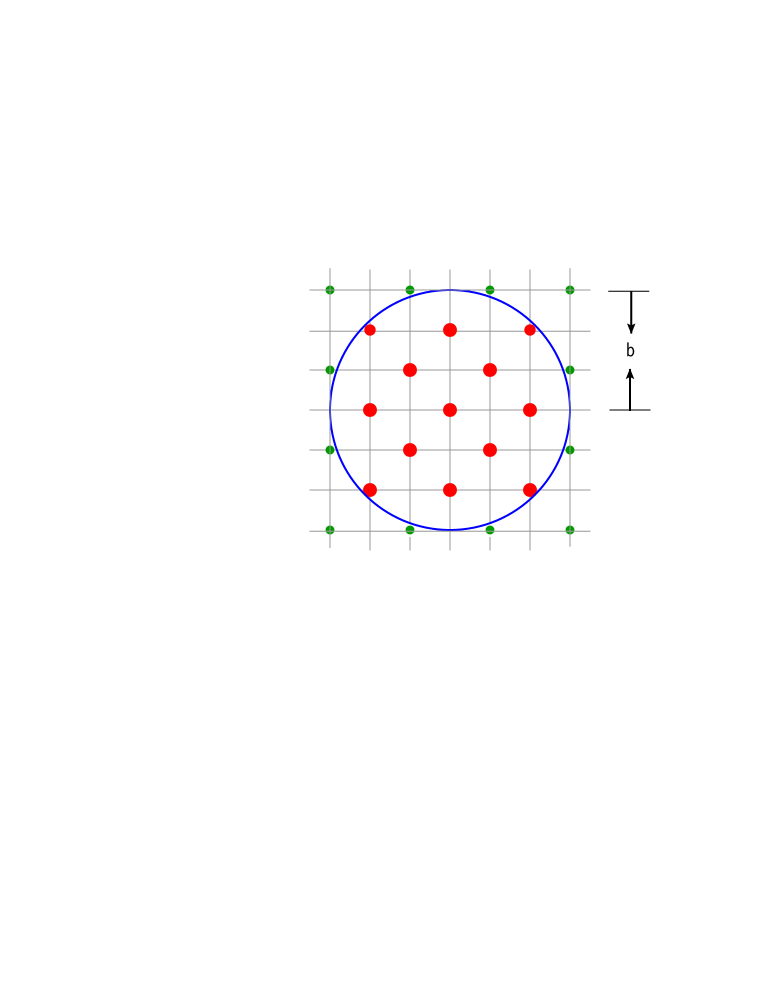
Figure 1: Due to the homogeneous and isotropic properties of our Universe, the particle number inside a chosen comoving volume should be a constant after the creation has been ceased. For the two pictures below, meanings are signified by colorized objects: the blue line is the comoving circle; red points are the particles inside the circle; green points are particles outside the circle; grey lines are the comoving coordinates. The left hand picture shows a younger Universe at $t_{0}$ old, and the chosen comoving circle has a comoving radius of $\mathrm{a}=\mathbb{R}\left(t_{0}\right)\ell$. The right hand picture is the same Universe but its age is $t_{0}+\Delta t$, and the comoving radius enlarges to $\mathrm{b}=\mathbb{R}\left(t_{0}+\Delta t\right)\ell$. Here, $\ell$ denotes the chosen comoving coordinate radius.

   

Next, to fit observations, we must introduce a proper model of inflaton into our discussion. We test result (29) by employing the classical chaotic model, $V\left(\phi\right)=\frac{1}{2}m_{\phi}^{2}\phi^{2}$. Since the remaining inflaton potential will become the energy density of ECC, as $V\left(\phi\left(t_{rest}\right)\right)=\frac{\Lambda}{8\pi G}$, $\Lambda$ and $N_{\mathrm{r}}\left(t_{rest}\right)$ will be found in expression

$$V^{{}^{\prime}}\left(\phi\left(t_{rest}\right)\right)=\pm\sqrt{\frac{m_{\phi}^{2}\Lambda}{4\pi G}}=-\sigma\left(t_{rest}\right)\ell^{-1}N_{\mathrm{r}}^{\nicefrac{{1}}{{3}}}\left(t_{rest}\right).$$ (30)

Here, the sign of “$\pm$” is dependent on the position of $\phi\left(t_{rest}\right)$. Additionally, it should be noted that $\left\rangle\sigma\left(t_{rest}\right)\right\langle$ is opposite to $\left\rangle\phi\left(t_{rest}\right)\right\langle$. Rewriting (30) clearly, the exact $\Lambda$-CPN relationship becomes

$$N_{\mathrm{r}}\left(t_{rest}\right)=\left(\frac{\ell^{2}m_{\phi}^{2}\Lambda}{4\pi G\sigma^{2}\left(t_{rest}\right)}\right)^{\nicefrac{{3}}{{2}}}.$$ (31)

III.2 Numerical results

III.2.1 The comoving entropy and the comoving particle number

Before we present the numerical result for the CPN and $\Lambda$, we should first outline the relationship between comoving entropy and the CPN. Nesteruk has come up with an applicable method and his result is that the particle number of a decoupled species inside a chosen adiabatic comoving volume is proportional to the decoupled species’ entropy as observed from the same volume (we call this comoving entropy for short) Thermal_inflation-2 . According to the Gibbs equation

$$T_{j}dS_{j}=d\left(\varepsilon_{j}v\right)+p_{j}dv,$$ (32)

we can easily have

$$T_{j}\frac{\dot{S}_{j}}{v}=\dot{\varepsilon}_{j}+\left(\varepsilon_{j}+p_{j}\right)\left(\frac{\dot{\mathbb{R}}}{\mathbb{R}}\right).$$ (33)

Here, $v=\left(\mathbb{R}\left(t\right)\ell\right)^{3}$ is the chosen comoving volume; $S_{j}\left(t\right)$ is the entropy for an arbitrary species $j$ inside the chosen comoving volume; and $T_{j}$ is the temperature defined by the density of species $j$. When the Universe is creating the species $j$, $S_{j}\left(t\right)$ increases simultaneously. Then, the entropy reaches a maximum constant when the creation of the species has ceased and the species itself has decoupled from others. In other words, the situation of $\dot{S}_{j}\left(t\geq t_{j,\,\mathrm{dec}}\right)=0$ means that there is no (net) energy current for the species $j$ between arbitrary comoving volumes. It also means that no energy transfer exists between species $j$ and other species inside the chosen comoving volume.

Of course, $\underset{l}{\sum}S_{l}$ will finally become a maximum constant to consist with the basic belief—the unique or adiabatic Universe—when the creation of all of species has ceased, even if some do not decouple from others. This is where the famous continuity equation of the Standard Model of Cosmology comes in.

Now, we adopt the example of a decoupling-neutrino. The following thermal equilibrium conditions are needed:

$$p_{\nu}\left(t\right) = \frac{\varepsilon_{\nu}\left(t\right)}{3},$$ (34)

$$\varepsilon_{\nu}\left(t\right) = \frac{\pi^{2}}{30}\cdot\frac{7}{8}\underset{\nu}{\sum}g_{\nu}T_{\nu}^{4}\left(t\right),$$ (35)

$$n_{\nu}\left(t\right) = \frac{\zeta\left(3\right)}{\pi^{2}}\cdot\frac{3}{4}\underset{\nu}{\sum}g_{\nu}T\nu^{3}\left(t\right),$$ (36)

at the cosmic time $t\gtrsim t_{\nu,\,\mathrm{dec}}$. Here $t_{\nu,\,\mathrm{dec}}\gtrsim 0.2\,\mathrm{s}$ is the decoupling time of the neutrino; the decoupling temperature is about $T_{\nu}\left(t\approx t_{\nu,\,\mathrm{dec}}\right)\simeq 1.5\,\mathrm{MeV}$ Neu-1 ; early_universe ; PFC ; $\underset{\nu}{\sum}g_{\nu}=6$ is the degree of freedom for neutrino species (3 flavors, 2 spin states each). The Gibbs equation for the decoupling-neutrino becomes

$$\left(T_{\nu}dS_{\nu}\right)_{t}\thickapprox 4.2\cdot\left(T_{\nu}dN_{\nu}\right)_{t}$$ (37)

in consideration of $N_{\nu}\left(t\right)=n_{\nu}\left(t\right)v\left(t\right)$.

However, we have no direct data for $S_{\nu}\left(t_{\mathrm{dec}}\right)$. Fortunately, we can substitute $S_{\nu}\left(t_{\mathrm{now}}\right)$ for $S_{\nu}\left(t_{\mathrm{dec}}\right)$, and vice versa since $\dot{S}_{\nu}\left(t\geq t_{\nu,\,\mathrm{dec}}\right)\approx 0$ . According to the estimate of entropy 1 ; entropy 2 , the entropy of cosmic-background neutrinos inside presently observable Universe is $S_{\mathrm{CBN}}^{obs}\left(t_{\mathrm{now}}\right)=s_{\mathrm{CBN}}\left(t_{\mathrm{now}}\right)\cdot v_{obs}\left(t_{\mathrm{now}}\right)=\left(5.16\pm 0.14\right)\times 10^{89}$. This is because the present day value of the CBN entropy density is

$$s_{\mathrm{CBN}}\left(t_{\mathrm{now}}\right) = \frac{2\pi^{2}}{45}\cdot\frac{7}{8}\underset{\nu}{\sum}g_{\nu}T_{\mathrm{CBN}}^{3}\left(t_{\mathrm{now}}\right)$$ (38)

$$= \left(1.411\pm 0.014\right)\times 10^{9}\,\mathrm{m^{-3}},$$

and the volume of today’s observable Universe early_universe is

$$v_{obs}\left(t_{\mathrm{now}}\right) = \frac{4}{3}\pi\left(\mathbb{R}\left(t_{\mathrm{now}}\right)\ell_{\mathrm{PH}}\right)^{3}$$ (39)

$$= \frac{4}{3}\pi\left(\mathbb{R}\left(t_{\mathrm{now}}\right)\int_{t_{\mathrm{Planck}}}^{t_{\mathrm{now}}}\frac{dt}{\mathbb{R}\left(t\right)}\right)^{3}$$

$$= \left(3.65\pm 0.10\right)\times 10^{80}\,\mathrm{m^{3}}.$$

(The present CBN temperature is $T_{\mathrm{CBN}}=\left(\nicefrac{{4}}{{11}}\right)^{\nicefrac{{1}}{{3}}}T_{\mathrm{CMB}}=\left(\nicefrac{{4}}{{11}}\right)^{\nicefrac{{1}}{{3}}}\cdot\left(2.725\pm 0.002\,\mathrm{K}\right)$. $\ell_{\mathrm{PH}}$ is the present particle horizon coordinate distance.) Therefore, the neutrino number was about $N_{\nu}\left(t_{\mathrm{dec}}\right)\approx 1.2\times 10^{89}$ inside the comoving volume of the present particle horizon coordinate distance ($v\left(t_{\nu,\,\mathrm{dec}}\right)\propto\left(\mathbb{R}\left(t_{\nu,\,\mathrm{dec}}\right)\ell_{\mathrm{PH}}\right)^{3}$) at the decoupling time $t_{\nu,\,\mathrm{dec}}$. Of course, the neutrino number inside the presently observable Universe ($v_{obs}\left(t_{\mathrm{now}}\right)\propto\left(\mathbb{R}\left(t_{\mathrm{now}}\right)\ell_{\mathrm{PH}}\right)^{3}$) is still $N_{\nu}\left(t_{\mathrm{now}}\right)\approx 1.2\times 10^{89}$.

One point worthy of attention is the fact that result (37) can be applied to CMB and WIMP dark matter ($S\approx 4N_{\mathrm{CMB\,or\,WDM}}$) because they are the known decoupled species. Of course, this requires the species of WDM to be a kind of fermion. And then we can employ the same thought to estimate these particle number inside the comoving volume for any chosen coordinate distance.

III.2.2 What is the $N_{\mathrm{r}}\left(t_{rest}\right)$?

Now, we have to talk about the role and essence of $N_{\mathrm{r}}\left(t_{rest}\right)$. In Section I, the words of “particle number” has defined as the sum of lepton, baryon (quark) and gauge boson number. However, we can also count the CPN by using the classification of the species of particles (such as photon, electron, neutrino, quark, and so on). Dependent on the consideration, the following statements should be highlighted to facilitate further discussion:

1. According to Subsection III.2.1, the CPN of an arbitrary decoupled species $j$ ($N\left(t_{j,\,\mathrm{dec}}\right)$) is proportional to its entropy ($S\left(t_{j,\,\mathrm{dec}}\right)$), which can be obtained from a chosen comoving volume ($\left(\mathbb{R}\left(t_{j,\,\mathrm{dec}}\right)\ell\right)^{3}$) at the time ($t_{j,\,\mathrm{dec}}$) when the species $j$ decouples from others. Moreover, we can conclude that no net energy current manifests between arbitrary comoving volumes inside the Universe, not only because the decoupled species has stopped its interactions with other species, but also due to the belief that our Universe is unique or adiabatic. Therefore, the entropy of a decoupled species inside a comoving volume should be a constant, even if the volume is expanding. This is equivalent to the other fact: namely that the CPN of an arbitrary decoupled species is also incontestably a constant.

2. Due to the spirit of the Bose-Einstein and Fermi-Dirac distributions, we can employ the temperature to relate the (energy or number) density of a relativistic species. On the other hand, a relativistic species’ density can be employed to relate the temperature of the species. (Here, the properties of $T_{\mathrm{b,\,f}}\left(t\right)\gg m_{\mathrm{b,\,f}}$ and $T_{\mathrm{b,\,f}}\left(t\right)\gg\mu_{\mathrm{b,\,f}}$ should be satisfied.) Thus, when a species $j$ drops out of thermal equilibrium, its temperature and density will evolve independently. This is the meaning of the “decoupling”. Since the system what we concern is adiabatic, the comoving entropy of the species $j$ will be a constant after its decoupling, namely, the CPN of the species $j$ will be also invariant. For this reason, we absolutely can employ the time of $t_{j,\,\mathrm{dec}}$ to represent the time while the species $j$ is ceased to produce, and the constant CPN of the species $j$ can be shown as $N\left(t_{j,\,\mathrm{dec}}\right)$. From the viewpoint of the particle physics, the decoupling of a species means that the species will no longer interact with others. It is of course that a decoupled species will not become another species.

3. Equations (29) and (30) remind us that the E(S)FF is dependent on $N_{\mathrm{r}}\left(t_{\left(rest\right)}\right)$. For this reason, any situation which can change this number will also weaken or strengthen the EFF. Of course, the value of the cosmological constant will be moved indirectly by the change of the CPN. (The situation of $\Lambda=0$ is a very special case that will be discussed in Subsection IV.2.2.) Thus, in our scenario, a fixed ECC implies that the Universe has a finite and constant CPN $N\left(t_{rest}\right)$. However, according to the $\Lambda$-CPN relationship (31), an observable variation of $\Lambda$ needs a sufficient number fluctuation to occur at the same cosmic time throughout the entire Universe. In other words, if the comoving number fluctuation is not enough, or the fluctuation is LOCAL (even if it is very big), the observable variation of $\Lambda$ will not be discovered by us or any alien.

Surely, the number $N_{\mathrm{r}}\left(t_{rest}\right)$ which appears in this paper means the TOTAL CPN, i.e.,

$$N_{\mathrm{r}}\left(t_{rest}\right)=\underset{j}{\sum}N\left(t_{j,\,\mathrm{dec}}\right)+\underset{l}{\sum}N_{l,\,\mathrm{int}}.$$ (40)

As we know, some species which still have interactions with others can be found in stars, the center of galaxies, our accelerators, nukes, and even in light bulbs (photons only) etc. Due to the facts, we can separate these species into the part of $\underset{l}{\sum}N_{l,\,\mathrm{int}}$. It is now known that if we ignore the case of neutrino oscillation, the lepton number and baryon (quark) number will be conserved after the GUT (grand unified theory) phase. Put simply, $\underset{l}{\sum}N_{l,\,\mathrm{int}}$ can be regarded as the constant for a big enough comoving volume. (Since, throughout the entire Universe, the energy density of the photons created by stars and humankind is too small.)

According to the present data, the estimate of WIMP dark matter $S_{\mathrm{WDM}}^{obs}\left(t_{\mathrm{now}}\right)$ is close to $2\times 10^{88\pm 1}$ entropy 1 ; CMB data supports $S_{\mathrm{CMB}}^{obs}\left(t_{\mathrm{now}}\right)\approx 5.4\times 10^{89}$ entropy 1 ; entropy 2 . Including the CBN comoving number, these provide a similar figure of $10^{89}$ inside the comoving volume ($\frac{4\pi}{3}\left(\mathbb{R}\left(t>t_{Ldec}\right)\ell_{\mathrm{PH}}\right)^{3}$, $t_{Ldec}$ is the decoupling time for the last decoupled species). On the other hand, the number density for presently “observable” baryon is about $n_{\mathrm{B}}\approx 0.11\,\mathrm{m^{-3}}$ (Fukugita et al., 1997 BND_1997 ) or $n_{\mathrm{B}}\approx 0.26\,\mathrm{m^{-3}}$ (Komatsu et al., 2010 WMAP7 ), which means that the number of baryons currently seen in cosmic gas, dust and stars inside the Universe is about $10^{79}$. Therefore, we can conclude that $N_{\mathrm{r}}\left(t_{rest}\right)\approx 10^{89\sim 90}$ is the total particle number which is the sum of these major parts of matter inside the comoving volume of $v_{\mathrm{PH}}\left(t\right)=\frac{4\pi}{3}\left(\mathbb{R}\left(t>t_{Ldec}\right)\ell_{\mathrm{PH}}\right)^{3}$.

III.2.3 Numerical results of the $\Lambda$-CPN relationship

Table 1: Numerical results for $G\sigma^{2}\left(t_{rest}\right)$ vs. $N_{\mathrm{r}}\left(t_{rest}\right)$ vs. $S_{\mathrm{r}}\left(t\approx t_{Ldec}\right)$. Inflaton mass is employed as $m_{\phi}=t_{\mathrm{Planck}}^{-1}\approx 1.855\times 10^{43}\,\mathrm{s^{-1}}$; the value of ECC is $\Lambda\approx 1.127\times 10^{-35}\,\mathrm{s^{-2}}$, which is dependent on the average present day value of the Hubble rate, $H_{\mathrm{now}}\approx 70\,\nicefrac{\mathrm{\nicefrac{\mathrm{km}}{\mathrm{s}}}}{\mathrm{Mpc}}$ acc:2011 . The comoving coordinate radius of the present particle horizon is defined as the unit length: $\ell_{\mathrm{PH}}\equiv 1$. The volume of the presently observable Universe is $v_{obs}\left(t_{\mathrm{now}}\right)=3.65\times 10^{80}\,\mathrm{m^{3}}$.

$\ell^{\>\dagger}$	$G\sigma^{2}\left(t_{rest}\right)$	$N_{\mathrm{r}}\left(t_{rest}\right)$	$S_{\mathrm{r}}\left(t_{Ldec}\right)$
$1$	$1$	$5.421\times 10^{75}$	$2.168\times 10^{76}$
$1$	$10^{-4}$	$5.421\times 10^{81}$	$2.168\times 10^{82}$
$1$	$10^{-9.2}$	$3.420\times 10^{89}$	$1.368\times 10^{90}$
$0.01$	$10^{-9.2}$	$3.420\times 10^{83}$	$1.368\times 10^{84}$

${}^{\dagger\;}\ell=1$ is the case of the present particle horizon coordinate distance.

Here, we provide numerical results in Table 1. These values are obtained by taking the value of inflaton mass and the observational data of $\Lambda$ into (31) and (37).

IV Probabilistic $\Lambda$ and the course of particle creation

IV.1 The behavior of $\sigma\left(t\right)$

In Section III, we define a RCRC, $\sigma\left(t\right)$, for describing the course of particle creation. As in the equations of (26), the requirement $\left\rangle\sigma\left(t\right)\right\langle=\left\rangle\dot{\phi}\left(t\right)\right\langle$ guarantees that $\left\rangle\mathrm{EKFF}\right\langle$ is always opposite to $\left\rangle\dot{\phi}\right\langle$. In addition, according to (30), if we employ $V\left(\phi\right)=\frac{1}{2}m_{\phi}^{2}\phi^{2}$ to consider the case of an oscillating inflaton, $\left\rangle\sigma\left(t_{rest}\right)\right\langle=-\left\rangle\phi\left(t_{rest}\right)\right\langle$ is included to insure $\left\rangle\mathrm{ESFF}\right\langle$ against the direction of the final restoring force $\left\rangle-V^{{}^{\prime}}\left(\phi\left(t_{rest}\right)\right)\right\langle$.

However, a sharp-eyed reader will find a discontinuous situation: there exists a case whereby $\left\rangle\sigma\left(t\right)\right\langle=-\left\rangle\sigma\left(t_{rest}\right)\right\langle$ when $\phi$ approaches to the static point $\phi\left(t_{rest}\right)$ (the relationship of time is $t\rightarrow t_{rest}$). All of the various behaviors when $t\rightarrow t_{rest}$ are listed in Table 2.

Table 2: This shows the relationship of signs (directions) which occur at the time when $t\rightarrow t_{rest}$. Here we employ the restoring force of $\phi$ as “$-\frac{dV\left(\phi\left(t\right)\right)}{d\phi}=-m_{\phi}^{2}\phi\left(t\right)$”.

$\left\rangle\sigma\left(t\right)\right\langle\;\>$	$\left\rangle\mathbf{f}_{\phi k}\right\langle\;\>$	$\left\rangle\sigma\left(t_{rest}\right)\right\langle\;\>$	$\left\rangle\mathbf{f}_{\phi s}\right\langle\;\>$	$\left\rangle\dot{\phi}\left(t\right)\right\langle\;\>$	$\left\rangle-m_{\phi}^{2}\phi\left(t\right)\right\langle\;\>$	$\left\rangle\phi\left(t_{rest}\right)\right\langle\;\>$	$\left\rangle-m_{\phi}^{2}\phi\left(t_{rest}\right)\right\langle$
$+$	$-$	$+$	$-$	$+$	$+$	$-$	$+$
$-$	$+$	$-$	$+$	$-$	$-$	$+$	$-$
$+$	$-$	$-$	$+$	$+$	$-$	$+$	$-$
$-$	$+$	$+$	$-$	$-$	$+$	$-$	$+$

The continuous situations between $\left\rangle\sigma\left(t\right)\right\langle$ and $\left\rangle\sigma\left(t_{rest}\right)\right\langle$ are shown in the two columns above the central line of Table 2. Meanwhile, the nethermost two columns are the discontinuous situations. Actually, discontinuous situations do not only happen in the example of the spring oscillating system from YCCHEN ; if we consider the question carefully, we will see that they also occur when $\phi$ approaches each and every turning point. However, even though the behavior of $\sigma\left(t\right)$ does not violate the laws of physics, we remain uncomfortable because the discontinuation means that Nature allows a $\sigma\left(t\right)$ which can suddenly change its sign but keep its value. Until now, a reasonable solution to explain these discontinuities has not been forthcoming. Fortunately, however, there does exist an intriguing mechanism for illustrating them. This unexpected result will be proposed in Subsection IV.2.

IV.2 The structure of $\sigma\left(t\right)$

IV.2.1 The structure of $\sigma\left(t\right)$ and the new inflaton field equation

Now, we will try to provide illustrations for the discontinuity of $\sigma\left(t\rightarrow t_{rest}\right)$ and the probabilistic result of $\phi\left(t_{rest}\right)=0$. According to (31), $N_{\mathrm{r}}\ggg 1$ and $\Lambda=0$ cannot occur simultaneously. However, if we employ the inflaton model in the form of $V\left(\phi\right)=\frac{1}{2}m_{\phi}^{2}\phi^{2}$ and consider that a maximum ESFF exists in inflaton dynamics, the discussion and conclusion of YCCHEN indicates that, because of (quantum) probability, it is possible for the final position of $\phi\left(t_{rest}\right)$ inside the “stagnant zone” to become zero. To account for this violation, a reasonable—if temporary—explanation is that the SRCRC $\sigma\left(t_{rest}\right)$ will become zero when $\phi\left(t_{rest}\right)$ is also zero. If this deduction works, a possible structure of RCRC is

$$\sigma\left(t\right)=u\left(t\right)\phi\left(t\right)+\varpi\left(t\right)\dot{\phi}\left(t\right),$$ (41)

where $u\left(t\right)$ and $\varpi\left(t\right)$ are two nonzero and undetermined coefficients, and their units are $\left[u\left(t\right)\right]=\mathrm{s^{-1}}$ and $\left[\varpi\left(t\right)\right]=\mathrm{1}$. The first property of $u\left(t\geq t_{rest}\right)=u\left(t_{rest}\right)$ must be satisfied for a fixed $\sigma\left(t_{rest}\right)$ to be constructed, but $\varpi\left(t\geq t_{rest}\right)$ does not necessarily have to be a constant, since a zero value of $\dot{\phi}\left(t\geq t_{rest}\right)$ means that $\varpi\left(t\right)\dot{\phi}\left(t\right)$ contributes nothing to $\sigma\left(t\geq t_{rest}\right)$. Then, a comparison with Table 2 and the analysis in Subsection IV.1 reveals that the conclusion

$$\left\rangle u\left(t\right)\right\langle=-,\quad\left\rangle\varpi\left(t\right)\right\langle=+$$ (42)

should be abided.

Therefore, the discontinuity worry of $\sigma\left(t\rightarrow t_{r}\right)$ as listed in Table 2 disappears due to the assumption of (41). This result derives from two facts: the powerful $\varpi\left(t_{\left\|\dot{\phi}\right\|>0}\right)\dot{\phi}\left(t_{\left\|\dot{\phi}\right\|>0}\right)$ makes $\sigma\left(t\right)$ become dependent on the (fast enough) rolling $\dot{\phi}$; and $\sigma\left(t_{\dot{\phi}\rightarrow 0}\right)$ is controlled by $-\left\|u\left(t_{\dot{\phi}\rightarrow 0}\right)\right\|\phi\left(t_{\dot{\phi}\rightarrow 0}\right)$. Besides, any discontinuous course (including those that emerge when $\phi$ approaches to every turning point) will have a situation of $\sigma\left(t\lesssim\tau_{j}\right)=0$ (where $\left\{\tau_{j}\right\}_{j=1,\,2,\,3,\,\cdots}$ is the set of times for these turning points). Thus, the EFF will become zero when $t$ runs to $\tau_{j}$. An explanation of this discovery is given in Subsection IV.2.3. Readers can also review a toy example in Figure 4, which will aid with picturing the EFF’s behavior.

Followingly, (21) will become the new inflaton field equation

$$\ddot{\phi}+\left(3H+\varpi\ell^{-1}N_{\mathrm{r}}^{\nicefrac{{1}}{{3}}}\right)\dot{\phi}+\left(V^{{}^{\prime}}\left(\phi\right)-\left\|u\right\|\ell^{-1}\phi N_{\mathrm{r}}^{\nicefrac{{1}}{{3}}}\right)=0$$ (43)

by introducing (24) and (41). It should be mentioned that $\ell$ is a constant chosen coordinate distance; $H$ and $N_{\mathrm{r}}$ must be functions of time; and $u\left(t\right)$ and $\varpi\left(t\right)$ are dependent on model selection. Clearly, (43) is consistent with the discussion of the dissipation term ($\Upsilon\dot{\phi}$, which has been mentioned in footnote 3) from the warm inflation scenario.

IV.2.2 The probabilistic $\Lambda$ and CPN

If we employ the example of $\phi\left(t_{rest}\right)=\pm\sqrt{\frac{\Lambda}{4\pi Gm_{\phi}^{2}}}$ from the classical chaotic model for our Universe, the result (31) will be transformed into

$$\Lambda=\frac{4\pi G}{m_{\phi}^{2}}\left(\left\|u_{\mathrm{our}}\left(t_{rest}\right)\right\|\ell^{-1}\phi\left(t_{rest}\right)N_{\mathrm{r}}^{\nicefrac{{1}}{{3}}}\left(t_{rest}\right)\right)^{2}$$ (44)

according to the last term of (43) when $\dot{\phi}\left(t_{rest}\right)=0$. Here $u_{\mathrm{our}}\left(t_{rest}\right)$ means that the coefficient is only for our Universe. From the relationship in (44), it looks as if the combination of $N_{\mathrm{r}}\ggg 1$ and $\Lambda=0$ will possibly occur, provided that $\phi\left(t_{rest}\right)=0$.

Now, two simpler questions require attention: What will happen to the Universe if $\left\|u\left(t\right)\right\|=\left\|u_{\dagger}\right\|$ for $t\geq t_{begin}$? How about if $\left\|\sigma\left(t\right)\right\|=\left\|\sigma_{\dagger}\right\|$ for $t\geq t_{begin}$?

We first give answer to the second question. It is obvious that the force relation of the oscillating $\phi$ is

$$\left\|V^{{}^{\prime}}\left(\phi\left(\tau_{j}\right)\right)\right\|\geq\left\|\mathbf{f}_{\phi k}\left(\tau_{j}\right)\right\|=\left\|\sigma_{\dagger}\right\|\ell^{-1}N_{\mathrm{r}}^{\nicefrac{{1}}{{3}}}\left(\tau_{j}\right),\quad\tau_{j}\leq t_{rest}$$ (45)

at every turning point $\phi\left(\tau_{j}\right)$ ($\left\{\tau_{j}\right\}_{j=1,\,2,\,3,\,\cdots}$ is the set of times for the turning points). Of course, $\phi\left(\tau_{j}\right)$ includes the last turning point—$\phi\left(t_{rest}\right)$. Employing $V\left(\phi\right)=\frac{1}{2}m_{\phi}^{2}\phi^{2}$, (45) becomes

$$m_{\phi}^{2}\left\|\phi\left(t_{rest}\right)\right\|=\left\|\sigma_{\dagger}\right\|\ell^{-1}N_{\mathrm{r}}^{\nicefrac{{1}}{{3}}}\left(t_{rest}\right)$$ (46)

when $N_{\mathrm{r}}\left(t_{rest}\right)$ becomes large enough at $\tau_{k}=t_{rest}$. Dependent on equation (46), the Universe has a nonzero exact ECC of

$$\Lambda=\frac{4\pi G}{m_{\phi}^{2}}\left(\left\|\sigma_{\dagger}\right\|\ell^{-1}N_{\mathrm{r}}^{\nicefrac{{1}}{{3}}}\left(t_{rest}\right)\right)^{2}.$$ (47)

Next, we will discuss the first question. Utilizing the model $V\left(\phi\right)=\frac{1}{2}m_{\phi}^{2}\phi^{2}$, the fact of the force relationship is

$$\left\|V^{{}^{\prime}}\left(\phi\left(\tau_{j}\right)\right)\right\|=m_{\phi}^{2}\left\|\phi\left(\tau_{j}\right)\right\|\geq\left\|u_{\dagger}\right\|\left\|\phi\left(\tau_{j}\right)\right\|\ell^{-1}N_{\mathrm{r}}^{\nicefrac{{1}}{{3}}}\left(\tau_{j}\right)$$ (48)

for every turning point $\phi\left(\tau_{j}\right)$ (where $\tau_{j}\leq t_{rest}$). Alternatively, the more clear relationship of (48) is

$$\left(m_{\phi}^{2}-\left\|u_{\dagger}\right\|\ell^{-1}N_{\mathrm{r}}^{\nicefrac{{1}}{{3}}}\left(\tau_{j}\right)\right)\left\|\phi\left(\tau_{j}\right)\right\|\geq 0.$$ (49)

Since the decreasing $\left\|\phi\left(t\right)\right\|$ provides a part of the energy to increase $N_{\mathrm{r}}\left(t\right)$, the restoring force will subsequently be canceled out by the fixed final EFF when $\tau_{j}\geq t_{rest}$, as

$$\left(m_{\phi}^{2}-\left\|u_{\dagger}\right\|\ell^{-1}N_{\mathrm{r}}^{\nicefrac{{1}}{{3}}}\left(t_{rest}\right)\right)\left\|\phi\left(t_{rest}\right)\right\|=0.$$ (50)

It is obvious that the simplest conditions of balance are:

1. $N_{\mathrm{r}}\left(t_{rest}\right)=\left(\frac{m_{\phi}^{2}}{\left\|u_{\dagger}\right\|\ell^{-1}}\right)^{3}$ for any possible $\left\|\phi\left(t_{rest}\right)\right\|$ which is lower than the maximum value, $\left\|\phi\left(t_{rest}\right)\right\|_{\mathrm{MAX}}$. Of course, this includes the situation of the minimum $\phi\left(t_{rest}\right)=0$. Unfortunately, the value of $\left\|\phi\left(t_{rest}\right)\right\|_{\mathrm{MAX}}$ cannot be provided here unless we have sufficient information about the energy transfer.

2. $\left\|\phi\left(t_{rest}\right)\right\|=0$ for any possible value of $N_{\mathrm{r}}\left(t_{rest}\right)$. This means that $N_{\mathrm{r}}\left(t_{rest}\right)<\left(\frac{m_{\phi}^{2}}{\left\|u_{\dagger}\right\|\ell^{-1}}\right)^{3}=N_{\mathrm{r}}\left(t_{rest}\right)_{\mathrm{MAX}}$ could occur. However, we also do not know the minimum value, $N_{\mathrm{r}}\left(t_{rest}\right)_{\mathrm{min}}$, here .

According to the above two illustrations, $\phi\left(t_{rest}\right)$ and $N_{\mathrm{r}}\left(t_{rest}\right)$ can be concluded as the probabilistic results that are restricted to the correspondingly necessary regions. This is consistent with the expectation of the probabilistic production of the cosmological constant YCCHEN .

IV.2.3 The decrease of CPN and the reversed “EKFF”

Following the above discussion of RCRC, a very important discovery should be mentioned. From the assumption of the dynamic RCRC in (41), it accords to have the situation of

$$\left\rangle\sigma\left(t\right)\right\langle=-\left\rangle\dot{\phi}\left(t\right)\right\langle$$ (51)

due to the contribution of a stronger “$-\left\|u\left(t\right)\right\|\phi\left(t\right)$” when the rolling $\phi$ approaches to every turning point of the $\phi$-system (while the relation of sign between $\phi$ and $\dot{\phi}$ is $\left\rangle\phi\left(t\right)\right\langle=\left\rangle\dot{\phi}\left(t\right)\right\langle$). Such an unabandonable property will destroy the order of Postulate B because we have

$$\dot{N}_{\mathrm{r}}\left(t\right)=\frac{3}{4}\chi^{\nicefrac{{4}}{{3}}}\ell^{3}\left(-\left\|u\left(t\right)\right\|\phi\left(t\right)+\varpi\left(t\right)\dot{\phi}\left(t\right)\right)\mathbb{R}^{4}\left(t\right)\dot{\phi}\left(t\right)$$ (52)

after combining (25) and (41). Equation (52) depicts how the CPN will be decreased when (51) (with the stronger “$-\left\|u\left(t\right)\right\|\phi\left(t\right)$”) happens. Fortunately, all of the ideas outlined in this paper are feasible, even if the temporary violation of Postulate B must be allowed in our scenario. Moreover, if the guess of RCRC, (41), can be extended to any model of inflaton potential, the corresponding Universe will also have some stages that the CPN will be decreased when $\left(-\left\|u\left(t\right)\right\|\phi\left(t\right)+\varpi\left(t\right)\dot{\phi}\left(t\right)\right)\dot{\phi}\left(t\right)<0$. In Appendix A, we offer a toy example to illustratively demonstrate the course of particle creation based on the assumption from (41).

A careful analysis of the situations corresponding to (51) reveals that the direction of EKFF ($\mathbf{f}_{\phi k}=-\sigma\left(t\right)\ell^{-1}N_{\mathrm{r}}^{\nicefrac{{1}}{{3}}}\left(t\right)$) will change at the stage of CPN decrease. It also asserts that the $\phi$-system can have several “frictionless” situations when $\phi\rightarrow\phi\left(\tau_{j}\right)$. Since the reversed “EKFF” weakens the restoring force $-V^{{}^{\prime}}\left(\phi\left(t\right)\right)$ when the rolling $\phi$ approaches to the turning point, it helps $\dot{\phi}$ to keep running longer. Subsequently, particles will begin to be created when $\phi$ starts to leave the turning point. Again, these processes are presented in an easily digestible form in the toy example from Appendix A.

IV.3 The meaning of $N_{\mathrm{r}}\left(t\right)$

Even though we have illustrated the FCPN by employing the classification of species in Subsection III.2.2, in this subsection, we should have a deeper discussion about the CPN from the point of the quantum numbers—lepton and baryon (quark) number. Especially, the discovery of the decrease of CPN can be found in our scenario. According to the definition at the beginning of this article, the name of particle number means the sum of lepton, baryon (quark) and gauge boson number. In addition, the standard model of particle physics tells us that the numbers of leptons and baryons will be conserved after the GUT phase transition. Therefore, except the primordial cosmic photons, the CPN can be determined as a constant after the GUT phase. (The gluon number is similar to baryon number since gluons will combine with quarks to become hadrons. Meanwhile, due to the electrical neutrality of our Universe, the number of electrons is also close to the number of quarks.) In other words, the lepton and baryon (quark) numbers will not change if the annihilations occur. A question arises naturally: what is the meaning of the decrease of the CPN indicated in the previous sections?

Table 3: The creation conditions of particles and anti-particles. The sign of $\pm$ denote the sign for the value of $\dot{\phi}\left(t\right)\cdot\dot{\phi}\left(t\right)$ and $-\phi\left(t\right)\cdot\dot{\phi}\left(t\right)$. In addition, $P$ represents the creation of particle, $AP$ represents the creation of anti-particle.

	$\quad\dot{\phi}\left(t\right)\quad$	$-\phi\left(t\right)$
$\quad\dot{\phi}\left(t\right)\quad$	$+$	$\quad+\qquad-\quad$
creation	$P$	$\quad P\qquad AP\quad$

In our opinion, the decrease presented in equation (52) can be illustrated by using the thought of anti-particle creation. To image the process of particle creation, if $\dot{N}_{\mathrm{r}}\left(t\right)>0$ represents the phenomenon that the creation rate of particles is larger than the rate of anti-particles, the course that the creation rate of anti-particles is more than the rate of particles can be indubitably denoted by $\dot{N}_{\mathrm{r}}\left(t\right)<0$. Moreover, if we regard neutrino as the Majorana particle, the numbers of neutrinos and cosmic photons will increase when their anti-particles create. For this reason, it seems that our discovery of equation (52) can provide the illustration in phenomenon for the fact that the numbers of baryons and electrons are much less than the numbers of photons and neutrinos.

Dependent on (52), the evolution equation of particle number, Table 3 can be made to indicate the conditions for particle and anti-particle creation. Clearly, the absolute positive term $\dot{\phi}\left(t\right)\cdot\dot{\phi}\left(t\right)$ creates particles throughout the creation course for any arbitrary situation of inflaton’s motion. However, the creation of anti-particles is controlled by the term of $-\dot{\phi}\left(t\right)\cdot\phi\left(t\right)$ only if the situation of $\left\rangle\dot{\phi}\left(t\right)\right\langle=\left\rangle\phi\left(t\right)\right\langle$ occurs. Moreover, it can easily discovered that the term of $\left\|u\left(t\right)\right\|\mathbb{R}^{4}\left(t\right)$ plays as the major role to define the amount of anti-particles. Therefore, from the research of phenomenon, the facts about anti-particle for its creation and less amount can be naturally obtained. In other words, it is possible to depict the evolution of the CPN and the scale factor during the creation epoch, if we can determine the terms of $u\left(t\right)$ and $\varpi\left(t\right)$.

Now, the conclusions of the CPN can be proposed from the point of the quantum number: 1. lepton, baryon (quark) and primordial gauge boson numbers will be ceased to create during the GUT phase transition; 2. the anti-particles will be created before the GUT phase transition to reduce the particle number; 3. the number of the Majorana particles will be increased when their anti-particles are created from the vacuum or the interactions of other species; 4. the final total CPN will become a constant after the stage of annihilation.

V Conclusions

To our surprise, the $\Lambda$-CPN relationship is very simple. According to equations (24), (25) and (31) , the following statements may be possible:

1. The guess of $\dot{N}_{\mathrm{r}}\left(t\right)=\alpha\left(t\right)\ell^{3}\mathbb{R}^{4}\left(t\right)\cdot\dot{\phi}\left(t\right)$ is correct. Additionally, when $t\geq t_{rest}$, CRC should become a constant of $\alpha\left(t_{rest}\right)$ to provide inflaton dynamics with a nonzero effective static frictional force, even if particles are no longer created.

2. According to (25), a static inflaton verifies why we have never observed any spontaneously created particle. In other words, the running inflaton controls the creation switch.

Moreover, through the analysis of RCRC, we obtain the following conclusions:

• The final results of the ECC $\Lambda$ and the CPN $N\left(t_{rest}\right)$ are probabilistic. Their values will fall into their own ranges. For $\Lambda$, the lowest minimum that can be allowed is zero, but the upper limit can not be provide at the present stage. In addition, the range of the CPN is $N\left(t_{rest}\right)_{\mathrm{min}}\leq N\left(t_{rest}\right)\leq\left(\frac{m_{\phi}^{2}}{\left\|u_{\dagger}\right\|\ell^{-1}}\right)^{3}$. However, the minimum value of the CPN can not be determined.

• We discover a new inflaton field equation of (43) which contains parameters of $N_{\mathrm{r}}\left(t\right)$ and “particle creation coefficients”. This equation shows that the EFF includes a dissipation term, a kind of damping force of inflaton, and a friction term which is dependent on whether the position of an inflaton can provide a static EFF to keep the (tiny) relic of inflaton potential remaining.

• Furthermore, since an inflaton still rolls after the end of inflation, a rolling inflaton which approaches to every turning point of the $\phi$-system will lead the “EKFF” to reverse. In phenomenon, such a process makes the decrease of CPN occur. This fact concludes that Postulate A is activated but Postulate B destroyed during the last phase of inflation. Equation (A) and the figures of Appendix A clearly show the evolution of the CPN. To this result, it possibly relates with the “course of antiparticle creation”. Due to the discovery of equation (52), the problem of the short of baryon number can be reasonably illustrated in phenomenon.

Comparing the estimates proposed by entropy 1 ; entropy 2 ; BND_1997 ; WMAP7 with our numerical results from Table 1, the evidence strongly indicates that the ECC is highly supported by contributions from the CPN of the decoupled species of CBN, CMB and WDM. Moreover, if the species of WDM is a kind of lepton or baryon, it is very possible that the CMB photon is the last decoupled species. Therefore, according to statement 3 of Subsection III.2.2 and conclusion 4 of Subsection IV.3, the CPN will become a constant when the course of $e^{\pm}$ annihilation ends. Moving forward, the ECC that we observe today has been stable since our Universe was a little more than $\mathbf{10^{0}}$ seconds old.

As for the result of the $10^{89}$ comoving particles which appear in the presently observable Universe, we should employ $G\sigma^{2}\left(t_{rest}\right)\approx 10^{-9}$ to connect the relationship between ECC and $N_{\mathrm{PH}}$ ($N_{\mathrm{PH}}$ is the particle number inside the comoving volume ($\frac{4\pi}{3}\left(\mathbb{R}\left(t>t_{Ldec}\right)\ell_{\mathrm{PH}}\right)^{3}$)). Is there any mystery of $G\sigma^{2}\left(t_{rest}\right)\approx 10^{-9}$? We will continue our research to find out the answer of the question.

Appendix A The course of particle creation: A toy case

Here, we would like to offer an example to show the process of particle creation. This is dependent on the assumption of (41) for RCRC. Again, it should be emphasized that the following example is a toy case designed to facilitate a smooth understanding of the effect of (41). We employ the CPN evolution equation

$$N_{\mathrm{r}}\left(t\right) = N_{\mathrm{r}}\left(t_{begin}\right)+$$

$$\frac{3}{4}\chi^{\nicefrac{{4}}{{3}}}\ell^{3}\int_{t_{begin}}^{t}\left(-\left\|u\left(t\right)\right\|\phi\left(t\right)+\varpi\left(t\right)\dot{\phi}\left(t\right)\right)\mathbb{R}^{4}\left(t\right)\dot{\phi}\left(t\right)dt$$

from integrating equation (25). For drawing pictures, the conditions

$$t_{begin}=1,\;\>N_{\mathrm{r}}\left(1\right)=25,\;\>\chi=0.8144,\;\>\ell=\ell_{\mathrm{PH}}=1,$$

$$\left\|u\left(t\right)\right\|=\varpi\left(t\right)=10^{10},$$

are necessary. Besides, we order the scale factor and scalar field as

$$\mathbb{R}\left(t\right)=\sqrt{t},$$

$$\dot{\phi}\left(t\right)=-\exp\left(-\frac{t-1}{4\pi}\right)\sin\left(\frac{t-1}{\sqrt{12\pi}}\right),\;\>\phi\left(1\right)\thickapprox 4.9567.$$

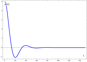
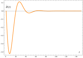
Figure 2: The evolution of scalar field $\phi\left(t\right)$.

   

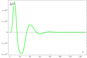
Figure 3: The evolution of effective friction.

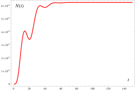
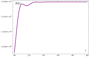
Figure 4: The evolution of particle number inside a chosen comoving volume.

   

The course of particle creation can be clearly observed from Figure 4. The EKFF reverses its direction from “$+$” to “$-$” for the first time at $t\approx 15$, while $\left\rangle\dot{\phi}\left(t<20\right)\right\langle=-$. Additionally, the result that the EKFF and $\dot{\phi}$ have the same direction at the same time i.e., $\left\rangle\mathrm{f}_{\phi k}\left(15<t<20\right)\right\langle=\left\rangle\dot{\phi}\left(15<t<20\right)\right\langle=-$, naturally follows. This causes the first instance of the decrease of CPN to occur.

Table 4: AN ILLUSTRATION OF SYMBOLS THAT APPEAR IN THIS PAPER

SYMBOL NAME	$\mathrm{UNIT^{\,\star}}$	$\mathrm{SIGN^{\>\ddagger}}$	MEANING
$t$ cosmic time	$\mathrm{s}$	$+$	$t_{begin}$ The time when inflation begins.
$G$ Newton’s gravitational constant	$\mathrm{s^{2}}$	$+$
$\ell$ comoving coordinate distance	$\mathrm{s}$	$+$	This is chosen and fixed. For more information see footnote 5.
$\mathbb{R}\left(t\right)$ spatial scale factor	$1$	$+$	$\mathbb{R}\left(t_{\mathrm{now}}\right)\equiv 1$.
$\mathrm{v}$ comoving coordinate volume	$\mathrm{s^{3}}$	$+$	$\mathrm{v}=\ell^{3}$
$v\left(t\right)$ comoving volume	$\mathrm{s^{3}}$	$+$	$v\left(t\right)=\left(\mathbb{R}\left(t\right)\ell\right)^{3}$ The proper volume.
$N\left(t\right)$ comoving particle number	$1$	$+$	Amount of particles inside a comoving volume.
$n\left(t\right)$ number density	$\mathrm{s^{-3}}$	$+$	$n\left(t\right)\equiv\frac{N\left(t\right)}{v\left(t\right)}$
$\varepsilon\left(t\right)$ energy density	$\mathrm{s^{-4}}$	$+$	$\varepsilon\left(t\right)\equiv\frac{E\left(t\right)}{v\left(t\right)}$; $E\left(t\right)$ is the comoving energy.
$p\left(t\right)$ pressure	$\mathrm{s^{-4}}$	$\pm$	$p_{\mathrm{DE}}<-\frac{\varepsilon_{\mathrm{DE}}}{3}$ for dark energy; $p_{\mathrm{r}}=\frac{\varepsilon_{\mathrm{r}}}{3}$ for radiation.
$H\left(t\right)$ Hubble rate	$\mathrm{s^{-1}}$	$\pm$	$H\left(t\right)\equiv\frac{\dot{\mathbb{R}}\left(t\right)}{\mathbb{R}\left(t\right)}$

$\phi\left(t\right)$ inflaton	$\mathrm{s^{-1}}$	$\pm$	A real scalar field; $\phi$ comes to rest at $t\geqslant t_{rest}$.
$m_{\phi}$ inflaton mass	$\mathrm{s^{-1}}$	$+$
$V\left(\phi\right)$ inflaton potential	$\mathrm{s^{-4}}$	$+$	$V\left(\phi\left(t_{rest}\right)\right)$ The remaining inflaton potential.
$\Lambda$ effective cosmological constant	$\mathrm{s^{-2}}$	$+$	$\Lambda=8\pi GV\left(\phi\left(t_{rest}\right)\right)$.
$T\left(t\right)$ temperature	$\mathrm{s^{-1}}$	$+$
$\mathrm{f}$ effective friction	$\mathrm{s^{-3}}$	$\pm$
$\alpha\left(t\right)$ coefficient of radiation creation	$\mathrm{s^{-2}}$	$\pm$	$\alpha\left(t_{rest}\right)$ is a constant called the SCRC.
$\sigma\left(t\right)$ reduced coefficient of radiation creation	$\mathrm{s^{-2}}$	$\pm$	$\sigma\left(t_{rest}\right)$ is a constant called the SRCRC.
$\chi$ particle number integral constant	$1$	$+$	$\chi\approx 0.8144$ Dependent on the thermal equilibrium condition.
$S$ comoving entropy	$1$	$+$	It is estimated from a chosen comoving volume.

^⋆ It is due to the unit choice that we adopt the Natural units: $c=k_{\mathrm{B}}=\hbar=1$.

^‡ We denote the sign or direction of $\Omega$ by using $\left\rangle\Omega\right\langle$.

References

- (1) A. Einstein, Kosmologische Betrachtungen zur allgemeinen Relativitätstheorie, Sitzungsberichte der esKöniglich Preußischen Akademie der Wissenschaften (Berlin), (1917) 142 [ECHO].
- (2) A. Friedman, Über die Krümmung des Raumes, Zeits. f. Physik 10 (1922) 377.
- (3) G. Lemaître, Un Univers homogène de masse constante et de rayon croissant rendant compte de la vitesse radiale des nébuleuses extra-galactiques, Annales de la Societe Scientifique de Bruxelles, A 47 (1927) 49 [NASA ADS].
- (4) E. Hubble, A relation between distance and radial velocity among extra-galactic nebulae, PNAS 15 (1929) 168.
- (5) Ya. B. Zel’dovich, The cosmological constant and the theory of elementary particles, Sov. Phys. Usp. 11 (1968) 381.
- (6) S. Weinberg, The cosmological constant problem, Rev. Mod. Phys. 61 (1989) 1.
- (7) A. G. Riess et al., Observational Evidence from Supernovae for an Accelerating Universe and a Cosmological Constant, Astron. J. 116 (1998) 1009 [astro-ph/9805201].
- (8) S. Perlmutter et al., Measurements of and from 42 High-Redshift Supernovae, Astrophys. J. 517 (1999) 565 [astro-ph/9812133].
- (9) S. Weinberg, The Cosmological Constant Problems (Talk given at Dark Matter 2000, February, 2000), [astro-ph/0005265].
- (10) A. H. Guth, Inflationary Universe: A possible solution to the horizon and flatness problems, Phys. Rev. D 23 (1981) 347.
- (11) A. Linde, Inflationary Cosmology, Lect. Notes Phys. 738 (2008) 1 [arXiv:0705.0164].
- (12) L. Kofman, A. Linde and A. Starobinsky, Reheating after Inflation, Phys. Rev. Lett. 73 (1994) 3195 [hep-th/9405187]; L. Kofman, A. Linde and A. Starobinsky, Towards the Theory of Reheating After Inflation, Phys. Rev. D 56 (1997) 3258 [hep-ph/9704452].
- (13) Y. Shtanov, J. Traschen and R. Brandenberger, Universe reheating after inflation, Phys. Rev. D 51 (1995) 5438 [hep-ph/9407247].
- (14) B. A. Bassett, S. Tsujikawa and D. Wands, Inflation Dynamics and Reheating, Rev. Mod. Phys. 78 (2006) 537 [astro-ph/0507632].
- (15) I. G. Moss, Primordial inflation with spontaneous symmetry breaking, Phys. lett. 75 (1985) 3218.
- (16) A. Berera and L.-Z. Fang, Thermally induced density perturbations in the inflation era, Phys. Rev. Lett. 74 (1995) 1912 [astro-ph/9501024]; A. Berera, I. G. Moss and R. O. Ramos, Warm Inflation and its Microphysical Basis, Rept. Prog. Phys. 72 (2009) 026901 [arXiv:0808.1855].
- (17) M. Bastero-Gil, A. Berera and R. O. Ramos, Dissipation coefficients from scalar and fermion quantum field interactions, JCAP 1109 (2011) 033 [arXiv:1008.1929].
- (18) I. G. Moss and C. Xiong, Dissipation coefficients for supersymmetric inflationary models, [hep-ph/0603266].
- (19) C. A. Egan and C. H. Lineweaver, A Larger Estimate of the Entropy of the Universe, Astrophys. J. 710 (2010) 1825 [arXiv:0909.3983v3].
- (20) P. Frampton et al., What is the entropy of the Universe? Class. Quant. Grav. 26 (2009) 145005 [arXiv:0801.1847v3].
- (21) M. Fukugita, C. J. Hogan and P. J. E. Peebles, The Cosmic Baryon Budget, Astrophys. J. 503 (1998) 518 [astro-ph/9712020].
- (22) E. Komatsu et al., Seven-Year Wilkinson Microwave Anisotropy Probe (WMAP) Observations: Cosmological Interpretation, Astrophys. J. Suppl. 192 (2011) 18 [arXiv:1001.4538].
- (23) A. G. Riess et al., A Solution: Determination of the Hubble Constant with the Hubble Space Telescope and Wide Field Camera , Astrophys. J. 730 (2011) 119 [arXiv:1103.2976].
- (24) E. Gunzig, R. Maartens and A. V. Nesteruk, Inflationary cosmology and thermodynamics, Class. Quant. Grav. 15 (1998) 923 [astro-ph/9703137].
- (25) A. V. Nesteruk, Inflationary Cosmology with Scalar Field and Radiation, Gen. Rel. Grav. 31 (1999) 983 [gr-qc/9905105].
- (26) I. Prigogine, J. Geheniau, E. Gunzig and P. Nardone, Thermodynamics and Cosmology, Gen. Rel. Grav. 21 (1989) 767.
- (27) V. Mukhanov, Physical Foundations of Cosmology, Cambridge University Press (Cambridge),2005.
- (28) E. W. Kolb and M. S. Turner, The Early Universe, Front. Phys. 69:1-547, 1990.
- (29) S. Hannestad and J. Madsen, Neutrino decoupling in the early Universe, Phys. Rev. D 52 (1995) 1764 [astro-ph/9506015].
- (30) Y.-C. Chen, The creation of radiation and the relic of inflaton potential, [arXiv:1109.6612].