Controlled stochastic networks in heavy traffic: Convergence of value functions

Abstract

Scheduling control problems for a family of unitary networks under heavy traffic with general interarrival and service times, probabilistic routing and an infinite horizon discounted linear holding cost are studied. Diffusion control problems, that have been proposed as approximate models for the study of these critically loaded controlled stochastic networks, can be regarded as formal scaling limits of such stochastic systems. However, to date, a rigorous limit theory that justifies the use of such approximations for a general family of controlled networks has been lacking. It is shown that, under broad conditions, the value function of the suitably scaled network control problem converges to that of the associated diffusion control problem. This scaling limit result, in addition to giving a precise mathematical basis for the above approximation approach, suggests a general strategy for constructing near optimal controls for the physical stochastic networks by solving the associated diffusion control problem.

and t1Supported in part by the NSF (DMS-10-04418), Army Research Office (W911NF-0-1-0080, W911NF-10-1-0158) and the US-Israel Binational Science Foundation (2008466). t2Supported in part by NSF Grant DMS-06-08634.

1 Introduction

As an approximation to control problems for critically-loaded stochastic networks, Harrison (in harri2 , see also harri1 , harri-canon ) has formulated a stochastic control problem in which the state process is driven by a multidimensional Brownian motion along with an additive control that satisfies certain feasibility and nonnegativity constraints. This control problem, that is, usually referred to as the Brownian Control Problem (BCP) has been one of the key developments in the heavy traffic theory of controlled stochastic processing networks (SPN). BCPs can be regarded as formal scaling limits for a broad range of scheduling and sequencing control problems for multiclass queuing networks. Finding optimal (or even near-optimal) control policies for such networks—which may have quite general non-Markovian primitives, multiple server capabilities and rather complex routing geometry—is in general prohibitive. In that regard, BCPs that provide significantly more tractable approximate models are very useful. In this diffusion approximation approach to policy synthesis, one first finds an optimal (or near-optimal) control for the BCP which is then suitably interpreted to construct a scheduling policy for the underlying physical network. In recent years there have been many works ata-kumar , bellwill , bellwill2 , BudGho , meyn , ward-kumar , chen-yao , dai-lin that consider specific network models for which the associated BCP is explicitly solvable (i.e., an optimal control process can be written as a known function of the driving Brownian motions) and, by suitably adapting the solution to the underlying network, construct control policies that are asymptotically (in the heavy traffic limit) optimal. The paper KuMa also carries out a similar program for the crisscross network where the state–space is three dimensional, although an explicit solution for the BCP here is not available.

Although now there are several papers which establish a rigorous connection between a network control problem and its associated BCP by exploiting the explicit form of the solution of the latter, a systematic theory which justifies the use of BCPs as approximate models has been missing. In a recent work BudGho2 it was shown that for a large family of Unitary Networks (following terminology of Will-Bram-2work , these are networks with a structure as described in Section 2), with general interarrival and service times, probabilistic routing and an infinite horizon discounted linear holding cost, the cost associated with any admissible control policy for the network is asymptotically, in the heavy traffic limit, bounded below by the value function of the BCP. This inequality, which provides a useful bound on the best achievable asymptotic performance for an admissible control policy, was a key step in developing a rigorous general theory relating BCPs with SPN in heavy traffic.

The current paper is devoted to the proof of the reverse inequality. The network model is required to satisfy assumptions made in BudGho2 (these are summarized above Theorem 2.10). In addition, we impose a nondegeneracy condition (Assumption 2.12), a condition on the underlying renewal processes regarding probabilities of deviations from the mean (Assumption 2.13) and regularity of a certain Skorohod map (Assumption 2.15) (see next paragraph for a discussion of these conditions). Under these assumptions we prove that the value function of the BCP is bounded below by the heavy traffic limit (limsup) of the value functions of the network control problem (Theorem 2.16). Combining this with the result obtained in BudGho2 (see Theorem 2.10), we obtain the main result of the paper (Theorem 2.18). This theorem says that, under broad conditions, the value function of the network control problem converges to that of the BCP. This result provides, under general conditions, a rigorous basis for regarding BCPs as approximate models for critically loaded stochastic networks.

Conditions imposed in this paper allow for a wide range of SPN models. Some such models, whose description is taken from Will-Bram-2work , are discussed in detail in Examples 1(a)–(c). We note that our approach does not require the BCP to be explicitly solvable and the result covers many settings where explicit solutions are unavailable. Most of the conditions that we impose are quite standard and we only comment here on three of them: Assumptions 2.5, 2.6 and 2.15. Assumption 2.5 says that each buffer is processed by at least one basic activity (see Remark 2.4). This condition, which was introduced in Will-Bram-2work , is fundamental for our analysis. In fact, Will-Bram-2work  has shown that without this assumption even the existence of a nonnegative workload matrix may fail. Assumption 2.6 is a natural condition on the geometry of the underlying network. Roughly speaking, it says that a nonzero control action leads to a nonzero state displacement. Assumption 2.15 is the third key requirement in this work. It says that the Skorohod problem associated with a certain reflection matrix $D$ [see equation (43) for the definition of $D$] is well posed and the associated Skorohod map is Lipschitz continuous. As Example 1 discusses, this condition holds for a broad family of networks (including all multiclass open queuing networks, as well as a large family of parallel server networks and job-shop networks).

The papers ata-kumar , bellwill , bellwill2 , BudGho , ward-kumar , dai-lin noted earlier, that treat the setting of explicitly solvable BCP, do much more than establish convergence of value functions. In particular, these works give an explicit implementable control policy for the underlying network that is asymptotically optimal in the heavy traffic limit. In the generality treated in the current work, giving explicit recipes (e.g., threshold type policies) is unfeasible, however, the policy sequence constructed in Section 4.1 suggests a general approach for building near asymptotically optimal policies for the network given a near optimal control for the BCP. Obtaining near optimal controls for the BCP in general requires numerical approaches (see, e.g., DuKu , Kushbook , meyn-book ), discussion of which is beyond the scope of the current work.

We now briefly describe some of the ideas in the proof of the main result—Theorem 2.16. We begin by choosing, for an arbitrary $\varepsilon>0$, a suitable $\varepsilon$-optimal control $\tilde{Y}$ for the BCP and then, using $\tilde{Y}$, construct a sequence of control policies $\{T^{r}\}_{r\geq 1}$ for the network model such that the (suitably scaled) cost associated with $T^{r}$ converges to that associated with $\tilde{Y}$, as $r\to\infty$. This yields the desired reverse inequality. One of the key difficulties is in the translation of a given control for the BCP to that for the physical network. Indeed, a (near) optimal control for the BCP can be a very general adapted process with RCLL paths. Without additional information on such a stochastic process, it is not at all clear how one adapts and applies it to a given network model. A control policy for the network needs to specify how each server distributes its effort among various job classes at any given time instant. By a series of approximations we show that one can find a rather simple $\varepsilon$-optimal control for the BCP, that is, easy to interpret and implement on a network control problem. As a first step, using PDE characterization results for general singular control problems with state constraints from AtBu (these, in particular, make use of the nondegeneracy assumption—Assumption 2.12), one can argue that a near-optimal control can be taken to be adapted to the driving Brownian motion and be further assumed to have moments that are subexponential in the time variable (see Lemma 3.10). Using results from BuRo , one can perturb this control so that it has continuous sample paths without significantly affecting the cost. Next, using ideas developed by Kushner and Martins KuMa in the context of a two-dimensional BCP, one can further approximate such a control by a process with a fixed (nonrandom) finite number of jumps that take values in a finite set. Two main requirements (in addition to the usual adaptedness condition) for such a process to be an admissible control of a BCP (see Definition 2.9) are the nonnegativity constraints (39) and state constraints (38). It is relatively easy to construct a pure jump process that satisfies the first requirement of admissibility, namely, the nonnegativity constraints, however, the nondegenerate Brownian motion in the dynamics rules out the satisfaction of the second requirement, that is, state constraints, without additional modifications. This is where the regularity assumption on a certain Skorohod map (Assumption 2.15) is used. The pure jump control is modified in a manner such that in between successive jumps one uses the Skorohod map to employ minimal control needed in order to respect state constraints. Regularity of the Skorohod problem ensures that this modification does not change the associated cost much. The Skorohod map also plays a key role in the weak convergence arguments used to prove convergence of costs. The above construction is the essential content of Theorem 3.5. The $\varepsilon$-optimal control that we use for the construction of the policy sequence requires two additional modifications [see part (iii) of Theorem 3.5 and below (59)] which facilitate adapting such a control for the underlying physical network and in some weak convergence proofs, but we leave that discussion for later in Section 3 (see Remark 3.6 and above Theorem 3.8).

Using a near-optimal control $\tilde{Y}$ of the form given in Section 3 (cf. Theorem 3.8), we then proceed to construct a sequence of policies $\{T^{r}\}$ for the underlying network. The key relation that enables translation of $\tilde{Y}$ into $\{T^{r}\}$ is (16) using which one can loosely interpret $\tilde{Y}(t)$ as the asymptotic deviation, with suitable scaling, of $T^{r}(t)$ from the nominal allocation $x^{*}t$ (see Definition 2.2 for the definition of nominal allocation vector). Recall that $\tilde{Y}$ is constructed by modifying, through a Skorohod constraining mechanism, a pure jump process (say, $\tilde{Y}_{0}$). In particular, $\tilde{Y}$ has sample paths that are, in general, discontinuous. On the other hand, note that an admissible policy $T^{r}$ is required to be a Lipschitz function (see Remark 2.8). This suggests the following construction for $T^{r}$. Over time periods (say, $\Delta t$) of constancy of $\tilde{Y}_{0}$ one should use the nominal allocation (i.e., $x^{*}\Delta t$), while jump-instants should be stretched into periods of length of order $r$ (note that in the scaled network, time is accelerated by a factor of $r^{2}$ and so such periods translate to intervals of length $1/r$ in the scaled evolution and thus are negligible) over which a nontrivial control action is employed as dictated by the jump vector (see Figure 4 for a more complete description). This is analogous to the idea of a discrete review policy proposed by Harrison bigstep (see also ata-kumar and references therein). There are some obvious difficulties with the above prescription, for example, a nominal allocation corresponds to the average behavior of the system and for a given realization is feasible only when the buffers are nonempty. Thus, one needs to modify the above construction to incorporate idleness, that is, caused due to empty buffers. The effect of such a modification is, of course, very similar to that of a Skorohod constraining mechanism and it is tempting to hope that the deviation process corresponding to this modified policy converges to $\tilde{Y}$ (in an appropriate sense), as $r\to\infty$. However, without further modifications, it is not obvious that the reflection terms that are produced from the idling periods under this policy are asymptotically consistent with those obtained from the Skorohod constraining mechanism applied to (the state process corresponding to) $\tilde{Y}_{0}$. The additional modification [see (4.1)] that we make roughly says that jobs are processed from a given buffer over a small interval $\Delta$, only if at the beginning of this interval there are a “sufficient” number of jobs in the buffer. This idea of safety stocks is not new and has been used in previous works (see, e.g., bellwill , bellwill2 , ata-kumar , BudGho , meyn-book ). The modification, of course, introduces a somewhat nonintuitive idleness even when there are jobs that require processing. However, the analysis of Section 4 shows that this idleness does not significantly affect the asymptotic cost. The above very rough sketch of construction of $T^{r}$ is made precise in Section 4.1.

The rest of the paper is devoted to showing that the cost associated with $T^{r}$ converges to that associated with $\tilde{Y}$. It is unreasonable to expect convergence of controls (e.g., with the usual Skorohod topology)—in particular, note that $T^{r}$ has Lipschitz paths for every $r$ while $\tilde{Y}$ is a (modification of) a pure jump process – however, one finds that the convergence of costs holds. This convergence proof, and the related weak convergence analysis, is carried out in Sections 4.2 and 4.3.

The paper is organized as follows. Section 2 describes the network structure, all the associated stochastic processes and the heavy-traffic assumptions as well as the other assumptions of the paper. The section also presents the SPN control problem, that is, considered here, along with the main result of the paper (Theorem 2.18). Section 3 constructs (see Theorem 3.8) a near-optimal control policy for the BCP which can be suitably adapted to the network control problem. In Section 4 the near-optimal control policy from Section 3 is used to obtain a sequence of admissible control policies for the scaled SPN. The main result of the section is Theorem 4.5, which establishes weak convergence of various scaled processes. Convergence of costs (i.e., Theorem 2.17) is an immediate consequence of this weak convergence result. Theorem 2.18 then follows on combining Theorem 2.17 with results of BudGho2 (stated as Theorem 2.10 in the current work). Finally, the Appendix collects proofs of some auxiliary results.

The following notation will be used. The space of reals (nonnegative reals), positive (nonnegative) integers will be denoted by $\mathbb{R}$ ($\mathbb{R}_{+}$), $\mathbb{N}$ ($\mathbb{N}_{0}$), respectively. For $m\geq 1$ and $\theta\in(0,\infty),$ $\mathcal{C}^{m}[\mathcal{C}^{m}_{\theta}]$ will denote the space of continuous functions from $[0,\infty)$ (resp. $[0,\theta]$) to $\mathbb{R}^{m}$ with the topology of uniform convergence on compacts (resp. uniform convergence). Also, $\mathcal{D}^{m}[\mathcal{D}^{m}_{\theta}]$ will denote the space of right continuous functions with left limits, from $[0,\infty)$ (resp. $[0,\theta]$) to $\mathbb{R}^{m}$ with the usual Skorohod topology. For $y\in\mathcal{D}^{m}$ and $t,\delta>0$, we write $\sup_{0\leq s\leq t}|y(s)|=|y|_{\infty,t}$ and $\sup_{0\leq s_{1}\leq s_{2}\leq t,|s_{1}-s_{2}|\leq\delta}|y(s_{1})-y(s_{2})|=\varpi_{y}^{t}(\delta)$, where for $z=(z_{1},\ldots,z_{m})^{\prime}\in\mathbb{R}^{m}$, $|z|^{2}=\sum_{i=1}^{m}|z_{i}|^{2}.$ All vector inequalities are to be interpreted component-wise. We will call a function $f\in\mathcal{D}^{m}$ nonnegative if $f(t)\geq 0$ for all $t\in{\mathbb{R}}_{+}$. A function $f\in\mathcal{D}^{m}$ is called nondecreasing if it is nondecreasing in each component. All (stochastic) processes in this work will have sample paths that are right continuous and have left limits, and thus can be regarded as $\mathcal{D}^{m}$-valued random variables with a suitable $m$. For a Polish space $\mathcal{E}$, $\mathcal{B}(\mathcal{E})$ will denote the corresponding Borel sigma-field. Weak convergence of $(\mathcal{E},\mathcal{B}(\mathcal{E}))$ valued random variables $Z_{n}$ to $Z$ will be denoted as $Z_{n}\Rightarrow Z$. Sequence of processes $\{Z_{n}\}$ is tight if and only if the measures induced by $Z_{n}$’s on $(\mathcal{D}^{m},\mathcal{B}(\mathcal{D}^{m}))$ form a tight sequence. A sequence of processes with paths in $\mathcal{D}^{m}$ ($m\geq 1$) is called $\mathcal{C}$-tight if it is tight in $\mathcal{D}^{m}$ and any weak limit point of the sequence has paths in ${\mathcal{C}}^{m}$ almost surely (a.s.). For processes $\{Z_{n}\}$, $Z$ defined on a common probability space, we say that $Z_{n}$ converge to $Z$, uniformly on compact time intervals (u.o.c.), in probability (a.s.) if for all $t>0$, $\sup_{0\leq s\leq t}|Z_{n}(s)-Z(s)|$ converges to zero in probability (resp. a.s.). To ease the notational burden, standard notation (that follow bram-will-1 , Will-Bram-2work ) for different processes are used (e.g., $Q$ for queue-length, $I$ for idle time, $W$ for workload process etc.). We also use standard notation, for example, $\bar{W},\hat{W}$, to denote fluid scaled, respectively, diffusion scaled, versions of various processes of interest [see (2) and (2)]. All vectors will be column vectors. An $m$-dimensional vector with all entries $1$ will be denoted by ${\mathbf{1}}_{m}$. For a vector $a$, $\operatorname{diag}(a)$ will denote the diagonal matrix such that the vector of its diagonal entries is $a$. $M^{\prime}$ will denote the transpose of a matrix $M$. Also, $C_{i},i=0,1,2,\ldots,$ will denote generic constants whose values may change from one proof to the next.

2 Multiclass queueing networks and the control problem

Let $(\Omega,\mathcal{F},\mathbb{P})$ be a probability space. All the random variables associated with the network model described below are assumed to be defined on this probability space. The expectation operation under $\mathbb{P}$ will be denoted by $\mathbb{E}$.

Network structure

We begin by introducing the family of stochastic processing network models that will be considered in this work. We closely follow the terminology and notation used in harri2 , harri1 , harri-canon , bellwill2 , Will-Bram-2work , bram-will-1 . The network has $\mathbf{I}$ infinite capacity buffers (to store $\mathbf{I}$ many different classes of jobs) and $\mathbf{K}$ nonidentical servers for processing jobs. Arrivals of jobs, given in terms of suitable renewal processes, can be from outside the system and/or from the internal rerouting of jobs that have already been processed by some server. Several different servers may process jobs from a particular buffer. Service from a given buffer $i$ by a given server $k$ is called an activity. Once a job starts being processed by an activity, it must complete its service with that activity, even if its service is interrupted for some time (e.g., for preemption by a job from another buffer). When service of a partially completed job is resumed, it is resumed from the point of preemption—that is, the job needs only the remaining service time from the server to get completed (preemptive-resume policy). Also, an activity must complete service of any job that it started before starting another job from the same buffer. An activity always selects the oldest job in the buffer that has not yet been served, when starting a new service [i.e., First In First Out (FIFO) within class]. There are $\mathbf{J}$ activities [at most one activity for a server-buffer pair $(i,k)$, so that $\mathbf{J}\leq\mathbf{I}\cdot\mathbf{K}$]. Here the integers $\mathbf{I},\mathbf{J},\mathbf{K}$ are strictly positive. Figure 1 gives a schematic for such a model.

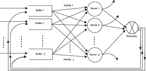
Figure 1: A network with $\mathbf{I}$ buffers, $\mathbf{J}$ activities, $\mathbf{K}$ servers and probabilistic routing (given by the matrix $P$).

Let $\mathbb{I}=\{1,\ldots,\mathbf{I}\}$, $\mathbb{J}=\{1,\ldots,\mathbf{J}\}$ and $\mathbb{K}=\{1,\ldots,\mathbf{K}\}$. The correspondence between the activities and buffers, and activities and servers are described by two matrices $C$ and $A$ respectively. $C$ is an $\mathbf{I}\times\mathbf{J}$ matrix with $C_{ij}=1$ if the $j$th activity processes jobs from buffer $i$, and $C_{ij}=0$ otherwise. The matrix $A$ is $\mathbf{K}\times\mathbf{J}$ with $A_{kj}=1$ if the $k$th server is associated with the $j$th activity, and $A_{kj}=0$ otherwise. Each activity associates one buffer and one server, and so each column of $C$ has exactly one 1 (and similarly, every column of $A$ has exactly one 1). We will further assume that each row of $C$ (and $A$) has at least one 1, that is, each buffer is processed by (server is processing, resp.) at least one activity. For $j\in\mathbb{J}$, let $\sigma(j)\equiv(\sigma_{1}(j),\sigma_{2}(j))=(i,k)$, if activity $j$ corresponds to the $k$th server processing class $i$ jobs. Let, for $k\in\mathbb{K}$, $\mathbb{J}(k)\doteq\{j\in\mathbb{J}\dvtx\sigma_{2}(j)=k\}$ and $\mathbb{I}(k)\doteq\{\sigma_{1}(j)\dvtx j\in\mathbb{J}(k)\}$. Thus, for the $k$th server, $\mathbb{J}(k)$ denotes the set of activities that the server can perform, and $\mathbb{I}(k)$ represents the corresponding buffers from which the jobs can be processed.

Stochastic primitives

We are interested in the study of networks that are nearly critically loaded. Mathematically, this is modeled by considering a sequence of networks $\{\mathcal{N}^{r}\}$ that “approach heavy traffic,” as $r\to\infty$, in the sense of Definition 2.2 below. Each network in the sequence has identical structure, except for the rate parameters that may depend on $r$. Here $r\in\mathbb{S}\subseteq{\mathbb{R}}^{+}$, where $\mathbb{S}$ is a countable set: $\{r_{1},r_{2},\ldots\}$ with $1\leq r_{1}<r_{2}<\cdots$ and $r_{n}\rightarrow\infty$, as $n\rightarrow\infty$. One thinks of the physical network of interest as the $r$th network embedded in this sequence, for a fixed large value of $r$. For notational simplicity, throughout the paper, we will write the limit along the sequence $r_{n}$ as $n\rightarrow\infty$ simply as “$r\rightarrow\infty$.” Also, $r$ will always be taken to be an element of $\mathbb{S}$ and, thus, hereafter the qualifier $r\in\mathbb{S}$ will not be stated explicitly.

The $r$th network $\mathcal{N}^{r}$ is described as follows. If the $i$th class ($i\in\mathbb{I}$) has exogenous job arrivals, the interarrival times of such jobs are given by a sequence of nonnegative random variables $\{u_{i}^{r}(n)\dvtx n\geq 1\}$ that are i.i.d with mean and standard deviation $1/{\alpha_{i}^{r}},\sigma_{i}^{u,r}\in(0,\infty)$ respectively. Let, by relabeling if needed, the buffers with exogenous arrivals correspond to $i\in\{1,\ldots,\mathbf{I}^{\prime}\}:=\mathbb{I}^{\prime}$, where $\mathbf{I}^{\prime}\leq\mathbf{I}$. We set ${\alpha_{i}^{r}},\sigma_{i}^{u,r}=0$ and $u^{r}_{i}(n)=\infty,n\geq 1$, for $i\in\mathbb{I}\setminus\mathbb{I}^{\prime}$. Service times for the $j$th type of activity (for $j\in\mathbb{J}$) are given by a sequence of nonnegative random variables $\{v_{j}^{r}(n)\dvtx n\geq 1\}$ that are i.i.d. with mean and standard deviation $1/{\beta_{j}^{r}},\sigma_{j}^{v,r}\in(0,\infty)$ respectively. We will assume that the above random variables are in fact strictly positive, that is,

$$\mbox{for all }i\in\mathbb{I},j\in\mathbb{J},\qquad\mathbb{P}\bigl{(}u^{r}_{i}(1)>0\bigr{)}=\mathbb{P}\bigl{(}v^{r}_{j}(1)>0\bigr{)}=1.$$ (1)

We will further impose the following uniform integrability condition:

the collection $$\{(u_{i}^{r}(1))^{2},(v_{j}^{r}(1))^{2};r\geq 1,j\in\mathbb{J},i\in\mathbb{I}^{\prime}\}$$ is uniformly integrable.

(2)

Rerouting of jobs completed by the $j$th activity is specified by a sequence of $(\mathbf{I}+1)$-dimensional vector $\{(\phi^{j,r}_{0}(n),\phi^{j,r}(n))^{\prime},n\geq 1\}$, where $\phi^{j,r}(n)=({\phi}^{j,r}_{i}(n)\dvtx i\in\mathbb{I})$. For each $j\in\mathbb{J}$ and $i\in\mathbb{I}\cup\{0\}$, ${\phi}^{j,r}_{i}(n)=1$ if the $n$th completed job by activity $j$ gets rerouted to buffer $i$, and takes the value zero otherwise, where $i=0$ represents jobs leaving the system. It is assumed that for each fixed $r$, $\{(\phi^{j,r}_{0}(n),\phi^{j,r}(n)),n\geq 1\}$, $j\in\mathbb{J}$, are (mutually) independent sequences of i.i.d $\operatorname{Multinomial}_{(\mathbf{I}+1)}(1,(p^{j}_{0},p^{j}))$, where $p^{j}=(p^{j}_{i}\dvtx i=1,\ldots,\mathbf{I})$. That, in particular, means, for $j\in\mathbb{J},n\geq 1$, $\sum_{i=0}^{\mathbf{I}}{\phi}^{j,r}_{i}(n)=\sum_{i=0}^{\mathbf{I}}p^{j}_{i}=1$. Furthermore, for fixed $j\in\mathbb{J},i_{1},i_{2}\in\mathbb{I}$,

$$\operatorname{Cov}(\phi_{i_{1}}^{j,r}(n),\phi_{i_{2}}^{j,r}(n))=\sigma^{\phi_{j}}_{i_{1}i_{2}}=-p_{i_{1}}^{j}p_{i_{2}}^{j}+p_{i_{1}}^{j}\delta_{i_{1},i_{2}},$$ (3)

where $\delta_{i_{1},i_{2}}$ is $1$ if $i_{1}=i_{2}$ and $0$ otherwise. We also assume that, for each $r$, the random variables

$$\{u_{i}^{r}(n),v_{j}^{r}(n),\phi^{j,r}_{0}(n),\phi^{j,r}(n),n\geq 1,i\in\mathbb{I},j\in\mathbb{J}\}$$ are mutually independent.

(4)

Next we introduce the primitive renewal processes, $(E^{r},S^{r})$, that describe the state dynamics. The process $(E^{r}_{1},\ldots,E^{r}_{\mathbf{I}^{\prime}})$ is the $\mathbf{I}^{\prime}$-dimensional exogenous arrival process, that is, for each $i\in\mathbb{I}^{\prime}$, $E_{i}^{r}(t)$ is a renewal process which denotes the number of jobs that have arrived to buffer $i$ from outside the system over the interval $[0,t]$. For class $i$ to which there are no exogenous arrivals (i.e., $i\in\mathbb{I}\setminus\mathbb{I}^{\prime}$), we set $E_{i}^{r}(t)=0$ for all $t\geq 0$. We will denote the process $(E^{r}_{1},\ldots,E^{r}_{\mathbf{I}})^{\prime}$ by $E^{r}$. For each activity $j\in\mathbb{J}$, $S_{j}^{r}(t)$ denotes the number of complete jobs that could be processed by activity $j$ in $[0,t]$ if the associated server worked continuously and exclusively on jobs from the associated buffer in $[0,t]$ and the buffer had an infinite reservoir of jobs. The vector $(S_{1}^{r},\ldots,S_{\mathbf{J}}^{r})^{\prime}$ is denoted by $S^{r}$. More precisely, for $i\in\mathbb{I},j\in\mathbb{J},m\geq 1$, let

$$\xi_{i}^{r}(m)\doteq\sum_{n=1}^{m}u_{i}^{r}(n),\qquad\eta_{j}^{r}(m)\doteq\sum_{n=1}^{m}v_{j}^{r}(n).$$ (5)

We set $\xi_{i}^{r}(0)=0,\eta_{j}^{r}(0)=0$. Then $E_{i}^{r}$, $S_{j}^{r}$ are renewal processes given as follows. For $t\geq 0$,

$$\qquad E_{i}^{r}(t)=\max\{m\geq 0\dvtx\xi_{i}^{r}(m)\leq t\},\quad S_{j}^{r}(t)=\max\{m\geq 1\dvtx\eta_{j}^{r}(m)\leq t\}.$$ (6)

Finally, we introduce the routing sequences. Let ${\bolds{\Phi}}^{j,r}_{i}(n)$ denote the number of jobs that are routed to the $i$th buffer, among the first $n$ jobs completed by activity $j$. Thus, for $i\in\mathbb{I},j\in\mathbb{J}$,

$${\bolds{\Phi}}^{j,r}_{i}(n)=\sum_{m=1}^{n}{\phi}_{i}^{j,r}(m),\qquad n=1,2,\ldots.$$ (7)

We will denote the $\mathbf{I}$-dimensional sequence $\{({\bolds{\Phi}}^{j,r}_{1}(n),\ldots,{\bolds{\Phi}}^{j,r}_{\mathbf{I}}(n))^{\prime}\}$ corresponding to routing of jobs completed by the $j$th activity by $\{{\bolds{\Phi}}^{j,r}(n)\}$. Also, ${\bolds{\Phi}}^{r}(n)$ will denote the $\mathbf{I}\times\mathbf{J}$ matrix $({\bolds{\Phi}}^{1,r}(n),{\bolds{\Phi}}^{2,r}(n),\ldots,{\bolds{\Phi}}^{\mathbf{J},r}(n))$.

Control

A Scheduling policy or control for the $r$th SPN is specified by a nonnegative, nondecreasing $\mathbf{J}$-dimensional process $T^{r}=\{(T_{1}^{r}(t),\ldots,T_{\mathbf{J}}^{r}(t))^{\prime},\allowbreak t\geq 0\}$. For any $j\in\mathbb{J},t\geq 0$, $T_{j}^{r}(t)$ represents the cumulative amount of time spent on the $j$th activity up to time $t$. For a control $T^{r}$ to be admissible, it must satisfy additional properties which are specified below in Definition 2.7.

State processes

For a given scheduling policy $T^{r}$, the state processes of the network are the associated $\mathbf{I}$-dimensional queue length process $Q^{r}$ and the $\mathbf{K}$-dimensional idle time process $I^{r}$. For each $t\geq 0$, $i\in\mathbb{I}$, $Q_{i}^{r}(t)$ represents the queue-length at the $i$th buffer at time $t$ (including the jobs that are in service at that time), and for $k=1,\ldots,\mathbf{K}$, $I_{k}^{r}(t)$ is the total amount of time the $k$th server has idled up to time $t$. Let $q^{r}=Q^{r}(0)\in\mathbb{N}^{\mathbf{I}}$ be the $\mathbf{I}$-dimensional vector of queue-lengths at time $0$. Note that, for $j\in\mathbb{J},t\geq 0$, $S_{j}^{r}(T_{j}^{r}(t))$ is the total number of services completed by the $j$th activity up to time $t$. The total number of completed jobs (by activity $j$) up to time $t$ that get rerouted to buffer $i$ equals ${\bolds{\Phi}}^{j,r}_{i}(S_{j}^{r}(T_{j}^{r}(t)))$. Recalling the definition of matrices $C$ and $A$, the state of the system at time $t\geq 0$ can be described by the following equations:

$$\hskip 30.0ptQ_{i}^{r}(t) = q^{r}+E_{i}^{r}(t)-\sum_{j=1}^{\mathbf{J}}{C}_{ij}S_{j}^{r}(T_{j}^{r}(t))+\sum_{j=1}^{\mathbf{J}}{{\bolds{\Phi}}^{j,r}_{i}}(S_{j}^{r}(T_{j}^{r}(t))),\qquad i\in\mathbb{I},$$ (8)

$$I_{k}^{r}(t) = t-\sum_{j=1}^{\mathbf{J}}{A}_{kj}T_{j}^{r}(t),\qquad k\in\mathbb{K}.$$ (9)

Heavy traffic

We now describe the main heavy traffic assumptionharri1 , harri-canon . We begin with a condition on the convergence of various parameters in the sequence of networks $\{\mathcal{N}^{r}\}$.

Assumption 2.1.

There are $q,\alpha,\sigma^{u}\in{\mathbb{R}}^{\mathbf{I}}_{+},\beta,\sigma^{v}\in{\mathbb{R}}^{\mathbf{J}}_{+}$, $\theta_{1}\in\mathbb{R}^{\mathbf{I}}$, $\theta_{2}\in\mathbb{R}^{\mathbf{J}}$ such that $\beta>0,\sigma^{v}>0$, $\alpha_{i},\sigma^{u}_{i}=0$ if and only if $i\in\mathbb{I}\setminus\mathbb{I}^{\prime}$, and, as $r\to\infty$,

$$\theta_{1}^{r} \doteq r({\alpha}^{r}-{\alpha})\rightarrow\theta_{1},\qquad\theta_{2}^{r}\doteq r({\beta^{r}}-\beta)\rightarrow\theta_{2},$$

$$\sigma^{u,r} \rightarrow \sigma^{u},\qquad\sigma^{v,r}\rightarrow\sigma^{v},\qquad\hat{q}^{r}\doteq\frac{q^{r}}{r}\rightarrow q.$$

The definition of heavy traffic, for the sequence $\{\mathcal{N}^{r}\}$, as introduced in harri1 (also see Will-Bram-2work , bram-will-1 , harri-canon ), is as follows.

Definition 2.2 ([Heavy traffic]).

Define $\mathbf{I}\times\mathbf{J}$ matrices $P^{\prime},R$, such that $P^{\prime}_{ij}\doteq p^{j}_{i}$, for $i\in\mathbb{I},j\in\mathbb{J}$, and

$$R\doteq(C-P^{\prime})\operatorname{diag}(\beta).$$ (11)

We say that the sequence $\{\mathcal{N}^{r}\}$ approaches heavy traffic as $r\to\infty$ if, in addition to Assumption 2.1, the following two conditions hold: [(ii)]

There is a unique optimal solution $(x^{*},\rho^{*})$ to the following linear program (LP):

$$\qquad\mbox{minimize }\rho\mbox{ such that }Rx={\alpha}\mbox{ and }Ax\leq\rho{\mathbf{1}}_{\mathbf{K}}\qquad\mbox{for all }x\geq 0.$$ (12)

The pair $(x^{*},\rho^{*})$ satisfies

$$\rho^{*}=1\quad\mbox{and}\quad Ax^{*}={\mathbf{1}}_{\mathbf{K}}.$$ (13)

Assumption 2.3.

The sequence of networks $\{\mathcal{N}^{r}\}$ approaches heavy traffic as $r\to\infty$.

Remark 2.4.

From Assumption 2.3, $x^{*}$ given in (i) of Definition 2.2 is the unique $\mathbf{J}$-dimensional nonnegative vector satisfying

$$Rx^{*}={\alpha},\qquad Ax^{*}={\mathbf{1}}_{\mathbf{K}}.$$ (14)

Following harri1 , assume without loss of generality (by relabeling activities, if necessary), that the first $\mathbf{B}$ components of $x^{*}$ are strictly positive (corresponding activities are referred to as basic) and the rest are zero (nonbasic activities). For later use, we partition the following matrices and vectors in terms of basic and nonbasic components:

$$x^{*}=\left[\matrix{x^{*}_{b}\cr\mathbf{0}}\right],\quad T^{r}=\left[\matrix{T^{r}_{b}\cr T^{r}_{n}}\right],\quad A=[B:N],\quad R=[H:M],$$ (15)

where $T^{r}$ is some control policy, ${\mathbf{0}}$ is a $(\mathbf{J}-\mathbf{B})$-dimensional vector of zeros, $B,N,H,M$ are $\mathbf{K}\times\mathbf{B}$, $\mathbf{K}\times(\mathbf{J}-\mathbf{B})$, $\mathbf{I}\times\mathbf{B}$ and $\mathbf{I}\times(\mathbf{J}-\mathbf{B})$ matrices, respectively.

The following assumption (see Will-Bram-2work ) says that for each buffer there is an associated basic activity.

Assumption 2.5.

For every $i\in\mathbb{I}$, there is a $j\in\mathbb{J}$ such that $R_{ij}>0$ and $x^{*}_{j}>0$.

Other processes

Components of the vector $x^{*}$ defined above can be interpreted as the nominal allocation rates for the $\mathbf{J}$ activities. Given a control policy $T^{r}$, define the deviation process $Y^{r}$ as the difference between $T^{r}$ and the nominal allocation:

$$Y^{r}(t)\doteq x^{*}t-T^{r}(t),\qquad t\geq 0.$$ (16)

It follows from (9) and (14) that the idle-time process $I^{r}$ has the following representation:

$$I^{r}(t)=AY^{r}(t),\qquad t\geq 0.$$

Let $\mathbf{N}\doteq\mathbf{K}+\mathbf{J}-\mathbf{B}$. Next we define a $\mathbf{N}\times\mathbf{J}$ matrix $K$ and $\mathbf{N}$-dimensional process $U^{r}$ as follows:

$$K\doteq\left[\matrix{B&N\cr 0&-\mathbb{I}}\right],\qquad U^{r}(t)\doteq KY^{r}(t),\qquad t\geq 0,$$ (17)

where $\mathbb{I}$ denotes a $(\mathbf{J}-\mathbf{B})\times(\mathbf{J}-\mathbf{B})$ identity matrix. Note that, with $T^{r}_{n}$ as in (15),

$$U^{r}(t)=\left[\matrix{I^{r}(t)\cr T^{r}_{n}(t)}\right],\qquad t\geq 0.$$ (18)

Finally, we introduce the workload process $W^{r}$ which is defined as a certain linear transformation of the queue-length process and is of dimension no greater than of the latter. More precisely, $W^{r}$ is an $\mathbf{L}$-dimensional process ($\mathbf{L}=\mathbf{I}+\mathbf{K}-\mathbf{B}$, see Will-Bram-2work ) defined as

$$W^{r}(t)=\Lambda Q^{r}(t),\qquad t\geq 0,$$ (19)

where $\Lambda$ is a $\mathbf{L}\times\mathbf{I}$-dimensional matrix with rank $\mathbf{L}$ and nonnegative entries, called the workload matrix. We will not give a complete description of $\Lambda$ since that requires additional notation; and we refer the reader to Will-Bram-2work , harri-canon for details. The key fact that will be used in our analysis is that there is a $\mathbf{L}\times\mathbf{N}$ matrix $G$ with nonnegative entries (see (3.11) and (3.12) in harri-canon ) such that

$$\Lambda R=GK.$$ (20)

We will impose the following additional assumption on $G$ which says that each of its columns has at least one strictly positive entry. The assumption is needed in the proof of Lemma 3.10 [see (3.1)].

Assumption 2.6.

There exists a $c>0$ such that for every $u\in{\mathbb{R}}_{+}^{\mathbf{N}}$, $|Gu|\geq c|u|$.

Rescaled processes

We now introduce two types of scalings. The first is the so-called fluid scaling, corresponding to a law of large numbers, and the second is the standard diffusion scaling, corresponding to a central limit theorem.

Fluid Scaled Process: This is obtained from the original process by accelerating time by a factor of $r^{2}$ and scaling down space by the same factor. The following fluid scaled processes will play a role in our analysis. For $t\geq 0$,

$$\bar{E}^{r}(t) \doteq r^{-2}E^{r}(r^{2}t),\qquad\bar{S}^{r}(t)\doteq r^{-2}S^{r}(r^{2}t),$$

$$\bar{\bolds{\Phi}}^{r}(t) \doteq r^{-2}{\bolds{\Phi}}^{r}(\lfloor r^{2}t\rfloor),\qquad\bar{T}^{r}(t)\doteq r^{-2}T^{r}(r^{2}t),$$ (21)

$$\bar{I}^{r}(t) \doteq r^{-2}I^{r}(r^{2}t),\qquad\bar{Q}^{r}(t)\doteq r^{-2}Q^{r}(r^{2}t).$$

Here for $x\in\mathbb{R}_{+}$, $\lfloor x\rfloor$ denotes its integer part, that is, the greatest integer bounded by $x$.

Diffusion Scaled Process: This is obtained from the original process by accelerating time by a factor of $r^{2}$ and, after appropriate centering, scaling down space by $r$. Some diffusion scaled processes that will be used are as follows. For $t\geq 0$,

$$\hat{E}^{r}(t) \doteq \frac{(E^{r}(r^{2}t)-{\alpha}^{r}r^{2}t)}{r},\qquad\hat{S}^{r}(t)\doteq\frac{(S^{r}(r^{2}t)-{\beta^{r}}r^{2}t)}{r},$$

$$\hat{\bolds{\Phi}}^{r}(t) \doteq \frac{({\bolds{\Phi}}^{r}(\lfloor r^{2}t\rfloor])-\lfloor r^{2}t\rfloor P^{\prime})}{r},$$

$$\hat{U}^{r}(t) \doteq r^{-1}U^{r}(r^{2}t),\qquad\hat{Q}^{r}(t)\doteq r^{-1}Q^{r}(r^{2}t),$$

$$\hat{W}^{r}(t) \doteq r^{-1}W^{r}(r^{2}t),\qquad\hat{Y}^{r}(t)\doteq r^{-1}Y^{r}(r^{2}t).$$

The processes $U^{r},Q^{r},W^{r}$ are not centered, as one finds (see Lemma 3.3 of BudGho2 ) that, with any reasonable control policy, their fluid scaled versions converge to zero as $r\rightarrow\infty$. Define for $t\geq 0$,

$$\hat{X}^{r}_{i}(t) \doteq \hat{E}^{r}_{i}(t)-\sum_{j=1}^{\mathbf{J}}(C_{ij}-p_{i}^{j})\hat{S}^{r}_{j}(\bar{T}^{r}_{j}(t))$$

$${}-\sum_{j=1}^{\mathbf{J}}\hat{\bolds{\Phi}}^{j,r}_{i}(\bar{S}^{r}_{j}(\bar{T}^{r}_{j}(t))),\qquad i\in\mathbb{I}.$$

Recall $\theta_{i}^{r}$ and $\hat{q}^{r}$ from Assumption 2.1. Using (8), (9), (14) and (17), one has the following relationships between the various scaled quantities defined above. For all $t\geq 0$,

$$\hat{Q}^{r}(t)=\hat{\zeta}^{r}(t)+R\hat{Y}^{r}(t),\qquad\hat{U}^{r}(t)=K\hat{Y}^{r}(t),$$

where

$$\hat{\zeta}^{r}(t)=\hat{q}^{r}+\hat{X}^{r}(t)+[\theta_{1}^{r}t-(C-P^{\prime})\operatorname{diag}(\theta_{2}^{r})\bar{T}^{r}(t)].$$ (24)

Also, using (19), (20) and (24), for all $t\geq 0$,

$$\quad\hat{W}^{r}(t)=\Lambda\hat{q}^{r}+\Lambda\hat{X}^{r}(t)+\Lambda[\theta_{1}^{r}t-(C-P^{\prime})\operatorname{diag}(\theta_{2}^{r})\bar{T}^{r}(t)]+G\hat{U}^{r}(t).$$ (25)

Admissibility of control policies

The definition of admissible policies (Definition 2.7), given below, incorporates appropriate nonanticipativity requirements and ensures feasibility by requiring that the associated queue-length and idle-time processes ($Q^{r},I^{r}$) are nonnegative.

For $m=(m_{1},\ldots,m_{\mathbf{I}})\in{\mathbb{N}}^{\mathbf{I}},n=(n_{1},\ldots,n_{\mathbf{J}})\in{\mathbb{N}}^{\mathbf{J}}$ we define the multiparameter filtration generated by interarrival and service times and routing variables as

$$\bar{\mathcal{F}}^{r}((m,n))$$

(26)

$$\qquad=\sigma\{u_{i}^{r}(m^{\prime}_{i}),v_{j}^{r}(n^{\prime}_{j}),\phi_{i}^{j,r}(n^{\prime}_{j})\dvtx m^{\prime}_{i}\leq m_{i},n^{\prime}_{j}\leq n_{j};i\in\mathbb{I},j\in\mathbb{J}\}.$$

Then $\{\bar{\mathcal{F}}^{r}((m,n))\dvtx m\in{\mathbb{N}}^{\mathbf{I}},n\in{\mathbb{N}}^{\mathbf{J}}\}$ is a multiparameter filtration with the following (partial) ordering:

$$(m^{1},n^{1})\leq(m^{2},n^{2})\quad\mbox{if and only if}\quad m^{1}_{i}\leq m^{2}_{i},n^{1}_{j}\leq n^{2}_{j};i\in\mathbb{I},j\in\mathbb{J}.$$

We refer the reader to Section 2.8 of Kurtz-redbook for basic definitions and properties of multiparameter filtrations, stopping times and martingales. Let

$$\bar{\mathcal{F}}^{r}\doteq\bigvee_{(m,n)\in{\mathbb{N}}^{\mathbf{I}+\mathbf{J}}}\bar{\mathcal{F}}^{r}((m,n)).$$ (27)

For all $(m,n)\in\{0,1\}^{\mathbf{I}+\mathbf{J}}$, we define $\bar{\mathcal{F}}^{r}((m,n))=\bar{\mathcal{F}}^{r}(({\mathbf{1}},{\mathbf{1}}))$ where ${\mathbf{1}}$ denotes the vector of 1’s. It will be convenient to allow for extra randomness, than that captured by $\bar{\mathcal{F}}^{r}$, in formulating the class of admissible policies. Let $\mathcal{G}$ be a $\sigma$-field independent of $\bar{\mathcal{F}}^{r}$. For $m\in\mathbb{N}^{\mathbf{I}},n\in\mathbb{N}^{\mathbf{J}}$, let $\mathcal{F}^{r}((m,n))\equiv{\mathcal{F}}^{r}_{\mathcal{G}}(m,n)\doteq\bar{\mathcal{F}}^{r}((m,n))\vee\mathcal{G}$.

Definition 2.7.

For a fixed $r$ and $q^{r}\in\mathbb{R}_{+}^{\mathbf{I}}$, a scheduling policy $T^{r}=\{(T_{1}^{r}(t),\ldots,T_{\mathbf{J}}^{r}(t))\dvtx t\geq 0\}$ is called admissible for $\mathcal{N}^{r}$ with initial condition $q^{r}$ if for some $\mathcal{G}$ independent of $\bar{\mathcal{F}}^{r}$, the following conditions hold: [(iii)]

$T^{r}_{j}$ is nondecreasing, nonnegative and satisfies $T^{r}_{j}(0)=0$ for $j\in\mathbb{J}$.

$I_{k}^{r}$ defined by (9) is nondecreasing, nonnegative and satisfies $I_{k}^{r}(0)=0$ for $k=1,\ldots,\mathbf{K}$.

$Q_{i}^{r}$ defined in (8) is nonnegative for $i\in\mathbb{I}$.

Define for each $r,t\geq 0$,

$${\sigma}^{r}_{0}(t) = (\sigma_{0}^{r,E}(t),\sigma_{0}^{r,S}(t))$$

$$\doteq \bigl{(}E_{i}^{r}(r^{2}t)+1\dvtx i\in\mathbb{I};S_{j}^{r}(T_{j}^{r}(r^{2}t))+1\dvtx j\in\mathbb{J}\bigr{)}.$$

Then, for each $t\geq 0$,

$${\sigma}^{r}_{0}(t)\mbox{ is a }\{\mathcal{F}^{r}((m,n))\dvtx m\in{\mathbb{N}}^{\mathbf{I}},n\in{\mathbb{N}}^{\mathbf{J}}\}\mbox{ stopping time}.$$ (29)

Define the filtration $\{\mathcal{F}^{r}_{1}(t)\dvtx t\geq 0\}$ as

$$\mathcal{F}^{r}_{1}(t) \!\doteq\! \mathcal{F}^{r}({\sigma}^{r}_{0}(t))$$

$$\!=\! \sigma\bigl{\{}A\in{\mathcal{F}}^{r}\dvtx A\cap\{{\sigma}^{r}_{0}(t)\leq(m,n)\}\in\mathcal{F}^{r}((m,n)),m\in{\mathbb{N}}^{\mathbf{I}},n\in{\mathbb{N}}^{\mathbf{J}}\bigr{\}}.$$

Then

$$\hat{U}^{r}\mbox{ is }\{\mathcal{F}^{r}_{1}(t)\}\mbox{-adapted}.$$ (31)

Denote by $\mathcal{A}^{r}(q^{r})$ the collection of all admissible policies for $\mathcal{N}^{r}$ with initial condition $q^{r}$.

Remark 2.8.

(i) and (ii) in Definition 2.7 imply, in view of (9) and properties of the matrix $A$, that

$$\qquad 0\leq T_{j}^{r}(t)-T_{j}^{r}(s)\leq t-s,\qquad j\in\mathbb{J}\mbox{ for all }0\leq s\leq t<\infty.$$ (32)

In particular, $T_{j}^{r}$ is a process with Lipschitz continuous paths. Condition (iv) in Definition 2.7 can be interpreted as a nonanticipativity condition. Proposition 2.8 and Theorem 5.4 of BudGho2 give general sufficient conditions under which this property holds (see also Proposition 4.1 of the current work).

Cost function

For the network $\mathcal{N}^{r}$, we consider an expected infinite horizon discounted (linear) holding cost associated with a scheduling policy $T^{r}$ and initial queue length vector $q^{r}$:

$$\quad J^{r}(q^{r},T^{r})\doteq\mathbb{E}\biggl{(}\int_{0}^{\infty}e^{-\gamma t}h\cdot\hat{Q}^{r}(t)\,dt\biggr{)}+\mathbb{E}\biggl{(}\int_{0}^{\infty}e^{-\gamma t}p\cdot d\hat{U}^{r}(t)\biggr{)}.$$ (33)

Here, $\gamma\in(0,\infty)$ is the “discount factor” and $h$, an $\mathbf{I}$-dimensional vector with each component $h_{i}\in(0,\infty),i\in\mathbb{I}$, is the vector of “holding costs” for the $\mathbf{I}$ buffers. In the second term, $p\geq 0$ is an $\mathbf{N}$-dimensional vector. The first $\mathbf{K}$ block of $U$ corresponds to the idleness process $I$, and, thus, the second term in the cost, in particular, captures the idleness cost. The last $\mathbf{J}-\mathbf{B}$ components of $U$ correspond to the time spent on nonbasic activities. Thus, this formulation of the cost allows, in addition to the idleness cost, the user to put a penalty for using nonbasic activities.

The formulation of the cost function considered in our work goes back to the original work of Harrison et al. harri1 , harri2 .

The scheduling control problem for $\mathcal{N}^{r}$ is to find an admissible control policy $T^{r}$ that minimizes the cost $J^{r}$. The value function $V^{r}$ for this control problem is defined as

$$V^{r}(q^{r})\doteq\inf_{T^{r}\in\mathcal{A}^{r}(q^{r})}J^{r}(q^{r},T^{r}),\qquad q^{r}\in\mathbb{N}_{0}^{\mathbf{I}}.$$ (34)

Brownian control problem

The goal of this work is to characterize the limit of value functions $V^{r}$ as $r\to\infty$, as the value function of a suitable diffusion control problem. In order to see the form of the diffusion control problem, we will like to send $r\to\infty$ in (24). Using the functional central limit theorem for renewal processes, it is easily seen that, for all reasonable control policies (see again Lemma 3.3 of BudGho2 ), when $\hat{q}^{r}$ converges to some $q\in\mathbb{R}_{+}^{\mathbf{I}}$, $\hat{\zeta}^{r}$ defined in (24) converges weakly to

$$\tilde{\zeta}=q+\tilde{X}+\theta\mathpzc{i},$$ (35)

where

$$\theta\doteq\theta_{1}-(C-P^{\prime})\operatorname{diag}(\theta_{2})x^{*}.$$ (36)

Here $\mathpzc{i}(s)=s,s\geq 0$ is the identity map and $\tilde{X}$ is a Brownian motion with drift 0 and covariance matrix

$$\Sigma\doteq\Sigma^{u}+(C-P^{\prime})\Sigma^{v}\operatorname{diag}(x^{*})(C-P^{\prime})^{\prime}+\sum_{j=1}^{\mathbf{J}}{\beta_{j}}x^{*}_{j}\Sigma^{\phi^{j}},$$ (37)

where $\Sigma^{u}$ is a $\mathbf{I}\times\mathbf{I}$ diagonal matrix with diagonal entries $(\sigma^{u}_{i})^{2},i\in\mathbb{I}$, $\Sigma^{v}$ is a $\mathbf{J}\times\mathbf{J}$ diagonal matrix with diagonal entries $(\sigma^{v}_{j})^{2},j\in\mathbb{J}$ and $\Sigma^{\phi^{j}}$s are $\mathbf{I}\times\mathbf{I}$ matrices with entries $\sigma^{\phi^{j}}_{i_{1}i_{2}},i_{1},i_{2}\in\mathbb{I}$ [see (3)]. Although the process $\hat{Y}^{r}$ in (24), for a general policy sequence $\{T^{r}\}$, need not converge, upon formally taking limit as $r\to\infty$, one is led to the following diffusion control problem.

Definition 2.9 ([Brownian Control Problem (BCP)]).

A $\mathbf{J}$-dimensional adapted process $\tilde{Y}$, defined on some filtered probability space $(\tilde{\Omega},\tilde{\mathcal{F}},\tilde{\mathbb{P}},\{\tilde{\mathcal{F}}(t)\})$ which supports an $\mathbf{I}$-dimensional $\{\tilde{\mathcal{F}}(t)\}$-Brownian motion $\tilde{X}$ with drift 0 and covariance matrix $\Sigma$ given by (37), is called an admissible control for the Brownian control problem with the initial condition $q\in\mathbb{R}_{+}^{\mathbf{I}}$ iff the following two properties hold $\tilde{\mathbb{P}}$-a.s.:

$$\tilde{Q}(t) \doteq \tilde{\zeta}(t)+R\tilde{Y}(t)\geq 0\qquad\mbox{where }\tilde{\zeta}(t)=q+\tilde{X}(t)+\theta t,t\geq 0,$$ (38)

$$\tilde{U} \doteq K\tilde{Y}\mbox{ is nondecreasing and }\tilde{U}(0)\geq 0,$$ (39)

where $\tilde{\zeta}$ and $\theta$ are as in (35) and (36) respectively. We refer to $\Phi=(\tilde{\Omega},\tilde{\mathcal{F}},\allowbreak\tilde{\mathbb{P}},\{\tilde{\mathcal{F}}(t)\},\tilde{X})$ as a system. We denote the class of all such admissible controls by $\tilde{\mathcal{A}}(q)$. The Brownian control problem is to

$$\mbox{infimize }\tilde{J}(q,\tilde{Y})\doteq\tilde{\mathbb{E}}\Biggl{[}\int_{0}^{\infty}e^{-\gamma t}h\cdot\tilde{Q}(t)\,dt+\int_{[0,{\infty})}e^{-\gamma t}p\cdot d\tilde{U}(t)\Biggr{]},$$ (40)

over all admissible controls $\tilde{Y}\in\tilde{\mathcal{A}}(q)$. Define the value function

$$\tilde{J}^{*}(q)=\inf_{\tilde{Y}\in\tilde{\mathcal{A}}(q)}\tilde{J}(q,\tilde{Y}).$$ (41)

Recall our standing assumptions (1), (2), (4), Assumptions 2.1, 2.3, 2.5 and 2.6. The following is the main result of BudGho2 .

Theorem 2.10 ((Budhiraja and Ghosh BudGho2 , Theorem 3.1, Corollary 3.2))

Fix $q\in\mathbb{R}_{+}^{\mathbf{I}}$ and for $r>0$, $q^{r}\in\mathbb{N}^{\mathbf{I}}$ such that $\hat{q}^{r}\to q$ as $r\to\infty$. Then

$$\liminf_{r\to\infty}V^{r}(q^{r})\geq\tilde{J}^{*}(q).$$

Remark 2.11.

The proof in BudGho2 is presented for the case where in the definition of $V^{r}(q^{r})$ [see (34)], $\mathcal{A}^{r}(q^{r})$ is replaced by the smaller family $\bar{\mathcal{A}}^{r}(q^{r})$ which consists of all $T^{r}\in\mathcal{A}^{r}(q^{r})$ that satisfy (iv) of Definition 2.7 with $\mathcal{F}^{r}((m,n))$ replaced by $\bar{\mathcal{F}}^{r}((m,n))$. Proof for the slightly more general setting considered in the current paper requires only minor modifications and, thus, we omit the details.

For the main result of this work, we will need additional assumptions.

Assumption 2.12.

The matrix $\Sigma$ is positive definite.

We will make the following assumption on the probabilities of deviations from the mean for the underlying renewal processes. Similar conditions have been used in previous works on construction of asymptotically optimal control policies bellwill , bellwill2 , BudGho , ata-kumar , dai-lin .

Assumption 2.13.

There exists $\bolds{\mathsf{m}}>2$ and, for each $\delta>0$, some $\varsigma(\delta)\in(0,\infty)$ such that, for $j\in\mathbb{J}$, $i\in\mathbb{I}$, $r\geq 1$, $t\in(1,\infty)$,

$$\mathbb{P}\bigl{(}|S_{j}^{r}(t)-\beta_{j}^{r}t|\geq\delta t\bigr{)} \leq \frac{\varsigma(\delta)}{t^{\bolds{\mathsf{m}}}},$$

$$\mathbb{P}\bigl{(}|E_{i}^{r}(t)-\alpha_{i}^{r}t|\geq\delta t\bigr{)} \leq \frac{\varsigma(\delta)}{t^{\bolds{\mathsf{m}}}},$$

$$\mathbb{P}\bigl{(}|\Phi_{i}^{j,r}(S_{j}^{r}(t))-p^{j}_{i}\beta_{j}^{r}t|\geq\delta t\bigr{)} \leq \frac{\varsigma(\delta)}{t^{\bolds{\mathsf{m}}}}.$$

The third inequality above is a consequence of the first two, but we note it explicitly here for future use. The assumption is clearly satisfied when $E_{i}$ and $S_{j}$ are Poisson processes. For general renewal processes, such inequalities hold under suitable moment conditions on the interarrival and service time distributions. Indeed, if for some $\bolds{\mathsf{m}}>1$

$$\mathbb{E}\Bigl{[}\sup_{r}[u_{i}^{r}(1)]^{2\bolds{\mathsf{m}}}\Bigr{]} < \infty,$$

$$\mathbb{E}\Bigl{[}\sup_{r}[v_{j}^{r}(1)]^{2\bolds{\mathsf{m}}}\Bigr{]} < \infty\qquad\mbox{for all }i\in\mathbb{I},j\in\mathbb{J},$$

then, from Theorem 4 of K-T , Assumption 2.13 is satisfied.

We now introduce an assumption on the regularity properties of a certain Skorohod map. This map plays a crucial role in our analysis; see proofs of Theorems 3.5 and 4.5 [see in particular, (58), (3.1), discussion below (91) and the proof of Theorem 3.8]. Let $\mathcal{D}_{+}^{\mathbf{I}}\doteq\{x\in\mathcal{D}^{\mathbf{I}}\dvtx x(0)\geq 0\}$ and

$$D=(C-P^{\prime})\operatorname{diag}(\beta)\operatorname{diag}(x^{*})C^{\prime}.$$ (43)

Definition 2.14.

Given $x\in\mathcal{D}_{+}^{\mathbf{I}}$, we say $(z,y)\in\mathcal{D}^{\mathbf{I}}\times\mathcal{D}^{\mathbf{I}}$ solve the Skorohod Problem (SP) for $(x,D)$ if: (i) $z(0)=x(0)$, (ii) $z=x+Dy$, (iii) $y$ is nondecreasing and $y(0)\geq 0$, (iv) $z(t)\geq 0$ for all $t\geq 0$, and(v) $\int_{[0,\infty)}1_{\{x_{i}(t)>0\}}\,dy_{i}(t)=0$ for all $i\in\mathbf{I}$.

Denoting by $\mathcal{D}_{0}$ the set of $x\in\mathcal{D}_{+}^{\mathbf{I}}$ such that there is a unique solution to the SP for $(x,D)$, we define maps $\Gamma\dvtx\mathcal{D}_{0}\to\mathcal{D}^{\mathbf{I}}$, $\hat{\Gamma}\dvtx\mathcal{D}_{0}\to\mathcal{D}^{\mathbf{I}}$ as $\Gamma(x)=z$, $\hat{\Gamma}(x)=y$ if $(z,y)$ solve the $SP$ for $(x,D)$.

Assumption 2.15.

$\mathcal{D}_{0}=\mathcal{D}_{+}^{\mathbf{I}}$ and the maps $\Gamma,\hat{\Gamma}$ are Lipschitz, namely, there exists $L\in(0,\infty)$ such that for all $x_{1},x_{2}\in\mathcal{D}_{+}^{\mathbf{I}}$,

$$\sup_{0\leq t<\infty}\{|\Gamma(x_{1})(t)-\Gamma(x_{2})(t)|+|\hat{\Gamma}(x_{1})(t)-\hat{\Gamma}(x_{2})(t)|\}\leq L\sup_{0\leq t<\infty}|x_{1}(t)-x_{2}(t)|.$$

We refer the reader to DupuisIshii1991 , Dup-Ram and har-rei for sufficient conditions under which the above regularity property of the Skorohod map holds. See also Example 1 below. For later use we introduce the notation $\bar{\Gamma}(x)=\operatorname{diag}(x^{*})C^{\prime}\hat{\Gamma}(x)$ for $x\in\mathcal{D}_{+}^{\mathbf{I}}$. Since $A$ has nonnegative entries and $x^{*}_{j}=0$ for $j=\mathbf{B}+1,\ldots,\mathbf{J}$, we see from the definition of $K$ [see (17)] that

$$\mbox{if }y=\bar{\Gamma}(x),\mbox{ then }Ky\geq 0.$$ (44)

For rest of the paper, in addition to the assumptions listed above Theorem 2.10, Assumptions 2.12, 2.13 and 2.15 will be in force. The main result of the paper is the following.

Theorem 2.16

Fix $q\in\mathbb{R}_{+}^{\mathbf{I}}$. Let for $r>0$, $q^{r}\in\mathbb{N}_{0}^{\mathbf{I}}$ be such that $\hat{q}^{r}\to q$ as $r\to\infty$. Then

$$\limsup_{r\to\infty}V^{r}(q^{r})\leq\tilde{J}^{*}(q).$$

The theorem is an immediate consequence of Theorem 2.17 below which is proved in Section 4. For $\varepsilon>0$, we say $Y\in\tilde{\mathcal{A}}(q)$ is $\varepsilon$-optimal for the BCP with initial value $q$ if

$$\tilde{J}(q,Y)\leq\tilde{J}^{*}(q)+\varepsilon.$$

When clear from the context, we will omit the phrase “for the BCP with initial value $q$” and merely say that $Y$ is $\varepsilon$-optimal.

Theorem 2.17

Fix $q\in\mathbb{R}_{+}^{\mathbf{I}}$. For $r>0$, let $q^{r}\in\mathbb{N}_{0}^{\mathbf{I}}$ be such that $\hat{q}^{r}\to q$ as $r\to\infty$. For every $\varepsilon>0$, there exists $\tilde{Y}\in\tilde{\mathcal{A}}(q)$, which is $\varepsilon$-optimal, and a sequence $T^{r}\in\mathcal{A}^{r}(q^{r})$, $r\geq 1$ such that

$$J^{r}(q^{r},T^{r})\to\tilde{J}(q,\tilde{Y})\qquad\mbox{as }r\to\infty.$$

Combining Theorems 2.10 and 2.16, the following is immediate.

Theorem 2.18

Fix $q\in\mathbb{R}_{+}^{\mathbf{I}}$. For $r>0$, let $q^{r}\in\mathbb{N}_{0}^{\mathbf{I}}$ be such that $\hat{q}^{r}\to q$ as $r\to\infty$. Then, as $r\to\infty$, $V^{r}(q^{r})\to\tilde{J}^{*}(q)$.

Assumptions made in this work can loosely be divided into two categories: Assumptions on the underlying stochastic primitives, which include, in particular, the heavy traffic conditions (Assumptions 2.1, 2.3, 2.12 and 2.13), and assumptions made on the network structure (Assumptions 2.5, 2.6 and 2.15). Below we discuss the validity of these structural assumptions for some basic families of SPN models.

Example 1.

The following examples have been described in detail in Will-Bram-2work . We will assume here, without loss of generality, that $\beta_{j}>0$ for all $j\in\mathbb{J}$ (an activity $j$ for which $\beta_{j}=0$ can simply be deleted from the network description). Furthermore, for all three settings considered below, Assumption 2.5 can be made without loss of generality, since otherwise one can consider a reduced system obtained by omitting the buffers that are not processed by any basic activity. Assumption 2.6 states that the matrix $G$ can be chosen in a manner such that it has no columns that are identically zero. Roughly speaking, it says that a nonzero control action leads to a nonzero state displacement. Although this appears to be a very natural geometric condition and is trivially satisfied for networks in part (a) below, it is not clear that it holds always for examples in parts (b) and (c) below. We will assume this condition to hold without further comment.

Thus, in discussion below, we will focus only on Assumption 2.15.

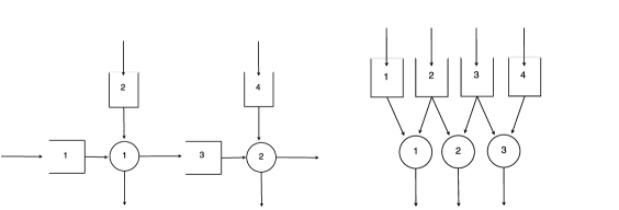
Figure 2: Open multiclass network (left) and parallel-server system (right).

Open multiclass queueing networks: These correspond to a setting where each buffer is processed by exactly one activity and, consequently, there is a one-to-one correspondence between activities and buffers, that is, $\mathbf{J}=\mathbf{I}$ (see left figure in Figure 2 for an example). For such networks, $R$ is an $\mathbf{I}\times\mathbf{I}$-matrix of the form $R=(\mathbb{I}-P^{\prime})\operatorname{diag}(\beta)$ where $P$ is a nonnegative matrix with spectral radius less than 1. In particular, $R$ is nonsingular, $K$ is a $\mathbf{K}\times\mathbf{J}$ matrix with full row rank and one can take $\Lambda=KR^{-1}$ and $G=\mathbb{I}$. Here $D=(\mathbb{I}-P^{\prime})\operatorname{diag}(\beta)\operatorname{diag}(x^{*})$ and from har-rei it is known that for such $D$ Assumption 2.15 is satisfied.

Parallel server networks: For such SPN, a buffer can be served by more than one activity, however, each job gets processed exactly once before leaving the system (i.e., there is no rerouting). See right figure in Figure 2 for an example. In particular, $P=0$ and, hence, $R=C\operatorname{diag}(\beta)$. In this case, $D=C\operatorname{diag}(\beta)\operatorname{diag}(x^{*})C^{\prime}\equiv\operatorname{diag}(\gamma^{*})$, where $\gamma^{*}_{i}=\sum_{j\dvtx\sigma_{1}(j)=i}\beta_{j}x^{*}_{j}$, for $i\in\mathbb{I}$. From Assumption 2.5 (which, as was noted above, can be made without loss of generality) we have that $\gamma^{*}>0$ and, thus, $D$ is a diagonal matrix with strictly positive diagonal entries. Assumption 2.15 is clearly satisfied for such matrices.

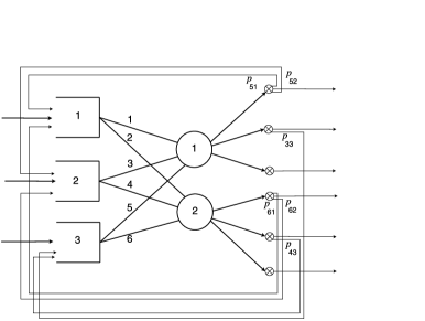
Figure 3: A Job-shop network. Here $p_{61}=p_{51}$, $p_{62}=p_{52}$, $p_{33}=p_{43}$.

Job-shop networks: This subclass of networks combines features of both (a) and (b): A buffer can be processed by more than one activity and jobs, once served, can get rerouted to another buffer for additional processing. See Figure 3 for an example. Following specific examples considered in Kumar (see also Will-Bram-2work ), we define job-shop networks as those which satisfy the following property: If for some $j,j^{\prime}\in\mathbb{J}$, and $i\in\mathbb{I}$, $\sigma_{1}(j)=\sigma_{1}(j^{\prime})=i$, then $p_{ji^{\prime}}=p_{j^{\prime}i^{\prime}}$ for all $i^{\prime}\in\mathbb{I}$. Namely, jobs corresponding to any two activities that process the same buffer $i$ have an identical (probabilistic) routing structure, following their completion by the respective servers. It is easily checked that in this case $D=(\mathbb{I}-\tilde{P^{\prime}})\operatorname{diag}(\gamma^{*})$, where $\gamma^{*}$ is as introduced in (b) and $\tilde{P}$ is an $\mathbf{I}\times\mathbf{I}$-dimensional matrix with entries $\tilde{p}_{i,i^{\prime}}=p_{j,i^{\prime}}$ where $j\in\mathbb{J}$ is such that $\sigma_{1}(j)=i$. Under the condition that $\tilde{P}$ has spectral radius less than 1, it follows from har-rei that Assumption 2.15 is satisfied.

3 Near-optimal controls for BCP

The rest of the paper is devoted to the proof of Theorem 2.17. Toward that goal, in this section we construct near-optimal controls for the BCP with certain desirable features. This construction is achieved in Theorem 3.8, which is the main result of this section.

Since an admissible control is not required to be of bounded variation, the BCP is a somewhat nonstandard diffusion control problem and is difficult to analyze directly. However, as shown in harri1 , under assumptions made in this paper, one can replace this control problem by an equivalent problem of Singular Control with State Constraints (SCSC). This control problem, also referred to as the Equivalent Workload Formulation (EWF) of the BCP, is given below. We begin by introducing the cost function, that is, optimized in this equivalent control problem.

Effective cost function: Recall the definition of the workload matrix $\Lambda$ introduced in (19). Let $\mathcal{W}\doteq\{\Lambda z\dvtx z\in{\mathbb{R}}_{+}^{\mathbf{I}}\}$. For each $w\in\mathcal{W}$, define

$$\hat{h}(w)\doteq\inf\{h\cdot q\dvtx\Lambda q=w,q\geq 0\}.$$ (45)

Since $h>0$, the infimum is attained for all $w\in\mathcal{W}$. It is well known (see Theorem 2 of bohm ) that one can take a continuous selection of the minimizer in the above linear program. That is, there is a continuous map $\tilde{q}^{*}\dvtx\mathcal{W}\to\mathbb{R}_{+}^{\mathbf{I}}$ such that

$$\tilde{q}^{*}(w)\in\mathop{\operatorname{argmin}}_{q}\{h\cdot q\dvtx\Lambda q=w,q\geq 0\}.$$ (46)

Thus, in particular, $\hat{h}$ is continuous. One can check that $\hat{h}$ satisfies linear lower and upper bounds. In order to see this, define

$$q^{*}(w)=\tilde{q}^{*}(w)1_{\{|w|\leq 1\}}+|w|\tilde{q}^{*}\biggl{(}\frac{w}{|w|}\biggr{)}1_{\{|w|>1\}}.$$ (47)

Then (46) holds with $\tilde{q}^{*}$ replaced by $q^{*}$. Since $\hat{h}(w)=h\cdot q^{*}(w)$ and $h>0$, we have from the above display that

$$b_{1}|w|-b_{2}\leq|\hat{h}(w)|\leq b_{3}(1+|w|),\qquad w\in\mathcal{W}$$ (48)

for some $b_{1},b_{2},b_{3}\in(0,\infty)$. Also, uniform continuity of $q^{*}$ on $\{w\in\mathcal{W}\dvtx|w|\leq 1\}$ shows that

$$|\hat{h}(w_{1})-\hat{h}(w_{2})|\leq\hat{m}(\delta)(1+|w_{1}|+|w_{2}|),$$

(49)

$$\eqntext{w_{1},w_{2}\in\mathcal{W},|w_{1}-w_{2}|\leq\delta.}$$ (50)

Here $\hat{m}$ is a modulus, that is, a nondecreasing function from $[0,\infty)\to[0,\infty)$ satisfying $\hat{m}(0+)=0$. Inequalities (48) and (3) will be used in order to appeal to some results from AtBu , BuRo (see Remark 3.4 below). Define

$$\mathcal{K}\doteq\{u\in{\mathbb{R}}^{\mathbf{N}}|u=Ky,y\in{\mathbb{R}}^{\mathbf{J}}\}.$$ (51)

The Equivalent Workload Formulation (EWF) and the associated control problem are defined as follows.

Definition 3.1 ([Equivalent Workload Formulation (EWF)]).

An $\mathbf{N}$-dimensional adapted process $\tilde{U}$, defined on some filtered probability space $(\tilde{\Omega},\allowbreak\tilde{\mathcal{F}},\tilde{\mathbb{P}},\{\tilde{\mathcal{F}}(t)\})$ which supports an $\mathbf{I}$-dimensional $\{\mathcal{F}(t)\}$-Brownian motion $\tilde{X}$ with drift 0 and covariance matrix $\Sigma$ defined in (37), is called an admissible control for the EWF with initial condition $w\in\mathcal{W}$ iff the following two properties hold $\tilde{\mathbb{P}}$-a.s.:

$$\mbox{$\tilde{U}$ is nondecreasing},\qquad\tilde{U}(0)\geq 0,\qquad\tilde{U}(t)\in\mathcal{K}\qquad\mbox{for all $t\geq 0$,}$$

$$\tilde{W}(t)\doteq w+\Lambda\theta t+\Lambda\tilde{X}(t)+G\tilde{U}(t)\in\mathcal{W}\qquad\mbox{for all }t\geq 0,$$

where $\theta$ is as in (36). We denote the class of all such admissible controls by $\tilde{\mathcal{A}}_{0}(w)$. The control problem for the EWF is to

$$\qquad\mbox{infimize }\tilde{J}_{0}(w,\tilde{U})\doteq\tilde{\mathbb{E}}\int_{0}^{\infty}e^{-\gamma t}\hat{h}(\tilde{W}(t))\,dt+\tilde{\mathbb{E}}\int_{[0,{\infty})}e^{-\gamma t}p\cdot d\tilde{U}(t),$$ (53)

over all admissible controls $\tilde{U}\in\tilde{\mathcal{A}}_{0}(w)$. Define the value function

$$\tilde{J}_{0}^{*}(w)=\inf_{\tilde{U}\in\tilde{\mathcal{A}}_{0}(w)}\tilde{J_{0}}(w,\tilde{U}).$$ (54)

From Theorem 2 of harri1 it follows that for all $w\in\mathcal{W},q\in{\mathbb{R}}_{+}^{\mathbf{I}}$ satisfying $w=\Lambda q$,

$$\tilde{J}^{*}(q)=\tilde{J}_{0}^{*}(w).$$ (55)

The following lemma will be used in order to appeal to some results from AtBu , BuRo . The proof is based on arguments in Will-Bram-2work . Let $\mathcal{K}_{+}=\mathcal{K}\cap\mathbb{R}^{\mathbf{N}}_{+}$.

Lemma 3.2

The cones $\mathcal{K}_{+}$ and $G\mathcal{K}_{+}$ have nonempty interiors and $\mathcal{W}^{o}\cap G\mathcal{K}_{+}\neq\varnothing$.

From Will-Bram-2work (see above Corollary 7.4 therein) it follows that $H$ has full row rank and so there is a $\mathbf{B}\times\mathbf{I}$ matrix $H^{{\dagger}}$ such that $HH^{{\dagger}}=\mathbb{I}$. Let $x_{b}=H^{{\dagger}}{\mathbf{1}}_{\mathbf{I}}$ and let $\varepsilon_{0}\in(0,\infty)$ be sufficiently small such that for all $\varepsilon\in(0,\varepsilon_{0}]$, $x^{\varepsilon}_{b}=x^{*}_{b}+\varepsilon x_{b}>0$. Let $\alpha_{0}=\alpha+\varepsilon_{0}{\mathbf{1}}_{\mathbf{I}}$ and $x_{0}=[x^{\varepsilon_{0}}_{b},{\mathbf{0}}]^{\prime}\in\mathbb{R}^{\mathbf{J}}$. Then $Rx_{0}=\alpha_{0}$. We will now argue that $\vartheta=\Lambda\alpha_{0}\in\mathcal{W}^{o}\cap(G\mathcal{K}_{+})^{o}$. Since the rows of $\Lambda$ are linearly independent, we can find an $\mathbf{I}\times\mathbf{L}$ matrix $\Lambda^{\dagger}$ such that $\Lambda\Lambda^{\dagger}=\mathbb{I}$. Fix $\delta=\frac{\varepsilon}{2|\Lambda^{\dagger}|}$. Then, whenever $\tilde{\vartheta}\in\mathbb{R}^{\mathbf{L}}$, $|\tilde{\vartheta}|<\delta$, we have $\alpha_{0}+\Lambda^{\dagger}\tilde{\vartheta}\in\mathbb{R}^{\mathbb{I}}_{+}$ and so $\vartheta+\tilde{\vartheta}=\Lambda(\alpha_{0}+\Lambda^{\dagger}\tilde{\vartheta})\in\mathcal{W}$. This shows that $\vartheta\in\mathcal{W}^{o}$. Next note that $\vartheta=\Lambda\alpha_{0}=\Lambda Rx_{0}=GKx_{0}.$ Since $Kx_{0}=Bx^{\varepsilon_{0}}_{b}$ and $x^{\varepsilon_{0}}_{b}>0$, we have that $Kx_{0}\in\mathcal{K}_{+}$ and so $\vartheta=GKx_{0}\in G\mathcal{K}_{+}$. Since $x^{\varepsilon_{0}}_{b}>0$, we can find $\varepsilon_{1}\in(0,\infty)$ such that whenever $\tilde{x}_{b}\in\mathbb{R}^{\mathbf{B}}$ is such that $|\tilde{x}_{b}|\leq\varepsilon_{1}$, $x^{\varepsilon_{0}}_{b}+\tilde{x}_{b}>0$. Now fix $\delta_{1}=\frac{\varepsilon_{1}}{|H^{{\dagger}}||\Lambda^{\dagger}|}$. Then, for any $\tilde{\vartheta}\in\mathbb{R}^{\mathbf{L}}$ with $|\tilde{\vartheta}|\leq\delta_{1}$ and $\tilde{x}=[H^{\dagger}\Lambda^{\dagger}\tilde{\vartheta},{\mathbf{0}}]^{\prime}\in\mathbb{R}^{\mathbf{J}}$,

$$\vartheta+\tilde{\vartheta}=\Lambda(\alpha_{0}+\Lambda^{\dagger}\tilde{\vartheta})=\Lambda(Rx_{0}+HH^{\dagger}\Lambda^{\dagger}\tilde{\vartheta})=\Lambda(Rx_{0}+R\tilde{x})=G\bigl{(}K(x_{0}+\tilde{x})\bigr{)}.$$

Since $|H^{\dagger}\Lambda^{\dagger}\tilde{\vartheta}|\leq\varepsilon_{1}$, we have $(x_{0}+\tilde{x})_{j}>0$ for all $j=1,\ldots,\mathbf{B}$. Also, $(x_{0}+\tilde{x})_{j}=0$ for all $j=\mathbf{B}+1,\ldots,\mathbf{J}$. Thus, $K(x_{0}+\tilde{x})\in\mathcal{K}_{+}$ and, therefore, $\vartheta+\tilde{\vartheta}\in G\mathcal{K}_{+}$. It follows that $\vartheta\in(G\mathcal{K}_{+})^{o}$.

Finally, we show that $\mathcal{K}_{+}^{o}\neq\varnothing$. Since $Ax^{*}={\mathbf{1}}_{\mathbf{K}}$, every row of $B$ must contain at least one strictly positive entry. Thus, $Bx^{\varepsilon_{0}}_{b}>0$. Choose $\varepsilon_{2}\in(0,\infty)$ sufficiently small such that $Bx^{\varepsilon_{0}}_{b}-\varepsilon_{2}N{\mathbf{1}}_{\mathbf{J}-\mathbf{B}}>0$. Let $\bar{x}=[x^{\varepsilon_{0}}_{b},-\varepsilon_{2}{\mathbf{1}}_{\mathbf{J}-\mathbf{B}}]^{\prime}\in\mathbb{R}^{\mathbf{J}}$. We now argue that $\bar{u}=K\bar{x}\in(\mathcal{K}_{+})^{o}$. Note that by construction $\bar{u}>0$. Thus, we can find $\varepsilon_{3}>0$ such that $\bar{u}+\tilde{u}\geq 0$ whenever $\tilde{u}\in\mathbb{R}^{\mathbf{N}}$ satisfies $|\tilde{u}|\leq\varepsilon_{3}$. Also, since $K$ has full row rank (see Corollary 6.2 of Will-Bram-2work ), we can find a $\mathbf{J}\times\mathbf{N}$ matrix $K^{\dagger}$ such that $KK^{\dagger}=\mathbb{I}$. Thus, $\bar{u}+\tilde{u}=K(\bar{x}+K^{\dagger}\tilde{u})$ and, consequently, $\bar{u}+\tilde{u}\in\mathcal{K}_{+}$. The result follows.

Note that the vector $x_{0}$ constructed in the proof of the lemma above has the property that $Rx_{0}>0$ and $Kx_{0}\geq 0$. Thus, we have shown the following:

Corollary 3.3

The set $\mathbb{T}=\{y\in\mathbb{R}^{\mathbf{J}}\dvtx Ky\geq 0,Ry>0\}$ is nonempty.

The above result will be used in the construction of a suitable near optimal control policy for the BCP [see below (59)].

Remark 3.4.

We will make use of some results from AtBu and BuRo that concern a general family of singular control problems with state constraints. We note below some properties of the model studied in the current paper that ensure that the assumptions of AtBu and BuRo are satisfied: [(a)]

$G$ has full row rank. This follows from the observation that $K,\Lambda$ and $R$ have full row ranks and, therefore,

$$\operatorname{rank}(G)=\operatorname{rank}(GK)=\operatorname{rank}(\Lambda R)=\operatorname{rank}(\Lambda)=\mathbf{L}.$$

$\mathcal{W}^{o}\cap(G\mathcal{K}_{+})^{o}\neq\varnothing$ and $\mathcal{K}_{+}$ has a nonempty interior (see Lemma 3.2).

$(Gu)\cdot{\mathbf{1}}_{\mathbf{L}}\geq|Gu|$, $u\cdot{\mathbf{1}}_{\mathbf{N}}\geq|u|$ for all $u\in\mathcal{K}_{+}$ and $w\cdot{\mathbf{1}}_{\mathbf{L}}\geq|w|$ for all $w\in\mathcal{W}$. This is an immediate consequence of the fact that the entries of $G$ and $\Lambda$ are nonnegative [see above (20)].

Since $\Lambda$ has full row rank and, by Assumption 2.12, $\Sigma$ is positive definite, we have that $\Lambda\Sigma\Lambda^{\prime}$ is positive definite. The above properties along with Assumption 2.6, (48) and (3) ensure that Assumptions of AtBu and BuRo are satisfied in our setting. In particular, Assumption (2.1)–(2.2) and (2.8)–(2.10) of AtBu hold in view of properties (b), (c) and (d) and equations (48) and (3). Similarly, Assumptions (1), (5) and 2.2 of BuRo hold in our setting [from property (c), (48) and Assumption 2.6, resp.]. Henceforth, when appealing to results from AtBu and BuRo , we will not make an explicit reference to these conditions.

Recall $\tilde{\zeta}(t)$ and the map $\bar{\Gamma}$ introduced above (35) and (44), respectively. The following is a key step in the construction of a near-optimal control with desirable properties.

Theorem 3.5

Fix $q\in\mathbb{R}_{+}^{\mathbf{I}}$. For each $\varepsilon\in(0,\infty)$, there exists $\tilde{Y}^{(1)}\in\tilde{\mathcal{A}}(q)$, given on some system $\Phi$, that is $\varepsilon$-optimal and has the following properties:

$$\tilde{Y}^{(1)}=\tilde{Y}_{0}^{(1)}+\bar{\Gamma}\bigl{(}\tilde{\zeta}+R\tilde{Y}_{0}^{(1)}\bigr{)},$$ (56)

where $\tilde{Y}_{0}^{(1)}$ is an adapted process with sample paths in $\mathcal{D}^{\mathbf{J}}$ satisfying the following: For some $T,\eta,M\in(0,\infty)$, $p_{0},j_{0}\in\mathbb{N}$, with $\theta=T/p_{0}$ and $\kappa=\theta/j_{0}$,

1. [(iii)]

2. $\tilde{Y}_{0}^{(1)}(t)=\tilde{Y}_{0}^{(1)}(n\theta)$ for $t\in[n\theta,(n+1)\theta),n=0,1,\ldots,p_{0}-1$ and $\tilde{Y}_{0}^{(1)}(t)=\tilde{Y}_{0}^{(1)}(p_{0}\theta)$ for $t\geq T=p_{0}\theta$.

3. Letting $\mathcal{S}_{M}^{\eta}=\{b\eta\dvtx b\in\mathbb{Z}^{\mathbf{J}},|b|\eta\leq M,Kb\geq 0\}$,

   $$\partial\tilde{Y}_{0}^{(1)}(n)\doteq\tilde{Y}_{0}^{(1)}(n\theta)-\tilde{Y}_{0}^{(1)}\bigl{(}(n-1)\theta\bigr{)}\in\mathcal{S}_{M}^{\eta},$$

   for $n=1,\ldots,p_{0}$ and $\partial\tilde{Y}_{0}^{(1)}(0)\doteq\tilde{Y}_{0}^{(1)}(0)=0$.

4. There is an i.i.d sequence of Uniform (over $[0,1]$) random variables $\{\tilde{\mathcal{U}}_{n}\}$, that is, independent of $\tilde{\zeta}$, and for each $n=1,\ldots,p_{0}$ a measurable map $\varpi_{n}\dvtx\mathbb{R}^{\mathbf{I}nj_{0}}\times[0,1]\to\mathcal{S}_{M}^{\eta}$, $n=1,\ldots,p_{0}$, such that the map $x\mapsto\varpi_{n}(x,t)$ is continuous, for a.e. $t$ in $[0,1]$, and

   $$\partial\tilde{Y}_{0}^{(1)}(n)=\varpi_{n}(\mathcal{X}^{\kappa}(n),\tilde{\mathcal{U}}_{n}),$$ (57)

   where $\mathcal{X}^{\kappa}(n)=\{\tilde{X}(\ell\kappa)\dvtx\ell=1,\ldots,nj_{0}\}$, $n=0,1,\ldots,p_{0}$.

Proof of Theorem 3.5 is given in Section 3.1.

Remark 3.6.

The above theorem provides an $\varepsilon$-optimal control $\tilde{Y}^{(1)}$, which is the “constrained”-version of a piecewise constant process $\tilde{Y}^{(1)}_{0}$. The value of $\tilde{Y}^{(1)}_{0}$ changes only at time-points that are integer multiples of $\theta$ and is constant for $t>T=p_{0}\theta$. Also, the changes in (the value of) the process occur in jumps with sizes that are integer multiples of some $\eta>0$ and are bounded by $M$. The third property in the theorem plays an important role in the weak convergence proof [Theorem 4.5, see, e.g., (4.3)] and says that the jump-sizes of this piecewise constant process are determined by the Brownian motion $\tilde{X}$ sampled at discrete instants $\{\kappa,2\kappa,\ldots\}$ and the independent random variable $\tilde{\mathcal{U}}_{n}$; furthermore, the dependence on $\tilde{X}$ is continuous. The continuous dependence is ensured using a mollification argument [see below (92)] that has previously been used in KuMa .

The following lemma is a straightforward consequence of the Lipschitz property of the Skorohod map, the linearity of the cost and the state dynamics. Proof is given in the Appendix.

Lemma 3.7

There is a $c_{1}\in(0,\infty)$ such that, if $q\in\mathbb{R}_{+}^{\mathbf{I}},T\in(0,\infty)$ and $\tilde{Y}^{1},\tilde{Y}^{2}\in\tilde{\mathcal{A}}(q)$ defined on a common filtered probability space are such that

$$\tilde{Y}^{i}(T+\cdot)-\tilde{Y}^{i}(T)=\bar{\Gamma}\bigl{(}\tilde{Q}^{i}(T)+\tilde{\zeta}(T+\cdot)-\tilde{\zeta}(T)\bigr{)},\qquad i=1,2,$$

where $\tilde{Q}^{i}$ is defined by the right-hand side of (38) by replacing $\tilde{Y}$ there by $\tilde{Y}^{i}$, then

$$|\tilde{J}(q,Y^{1})-\tilde{J}(q,Y^{2})|\leq c_{1}\mathbb{E}|Y^{1}-Y^{2}|_{\infty,T}.$$

Define $\vartheta\dvtx\mathbb{R}_{+}^{\mathbf{I}}\times\mathbb{R}^{\mathbf{J}}\to\mathbb{R}^{\mathbf{J}}$ as

$$\vartheta(q_{0},y)=y+\bar{\Gamma}(q_{0}+Ry\mathpzc{i})(1),\qquad q_{0}\in\mathbb{R}_{+}^{\mathbf{I}},y\in\mathbb{R}^{\mathbf{J}}.$$

Note that $\vartheta$ is a Lipschitz map: that is, for some $\vartheta_{\mathrm{lip}}\in(0,\infty)$, we have for $(q_{0},y),(\tilde{q}_{0},\tilde{y})\in\mathbb{R}_{+}^{\mathbf{I}}\times\mathbb{R}^{\mathbf{J}}$,

$$|\vartheta(q_{0},y)-\vartheta(\tilde{q}_{0},\tilde{y})|\leq\vartheta_{\mathrm{lip}}(|q_{0}-\tilde{q}_{0}|+|y-\tilde{y}|).$$ (58)

Also, since $\vartheta(q_{0},0)=0$, we have for $(q_{0},y)\in\mathbb{R}_{+}^{\mathbf{I}}\times\mathbb{R}^{\mathbf{J}}$,

$$|\vartheta(q_{0},y)|\leq\vartheta_{\mathrm{lip}}|y|.$$ (59)

We now present the near-optimal control that will be used in the proof of Theorem 2.17. Recall the set $\mathbb{T}$ introduced in Corollary 3.3. Fix $\varepsilon>0$, and a unit vector $y^{*}\in\mathbb{T}$ and define $c_{2}\in[1,\infty)$ as

$$c_{2}=\max\bigl{\{}2c_{1}(p_{0}+1)\bigl{(}1+L|\operatorname{diag}(x^{*})C^{\prime}|\bigr{)}|Ry^{*}|,1\bigr{\}}.$$

Let $\tilde{Y}_{0}^{(1)}$, $\tilde{Y}^{(1)}$ be as in Theorem 3.5 with $\varepsilon=\varepsilon/2$. Let $\varepsilon_{0}=\varepsilon/c_{2}$ and define $\vartheta_{\varepsilon_{0}}(x,y)=\vartheta(x,y)+\varepsilon_{0}y^{*}$. Define control process $\tilde{Y}\in\tilde{\mathcal{A}}(q)$ with the corresponding state process $\tilde{Q}$ [defined by the right-hand side of (38)] by the following equations. For $n=0,1,\ldots,p_{0}$,

$$\tilde{Y}(n\theta)-\tilde{Y}(n\theta-)=\vartheta_{\varepsilon_{0}}(\tilde{Q}(n\theta-),\partial\tilde{Y}_{0}^{(1)}(n)),$$ (60)

and

$$\qquad\quad\tilde{Y}(t+n\theta)-\tilde{Y}(n\theta)=\bar{\Gamma}\bigl{(}\tilde{Q}(n\theta)+\tilde{\zeta}(\cdot+n\theta)-\tilde{\zeta}(n\theta)\bigr{)}(t),\qquad t\in[0,\theta),$$ (61)

with the conventions that for $n=p_{0}$, $[0,\theta)$ is replaced by $[0,\infty)$ and for $n=0$, $\tilde{Q}(n\theta-)=q$. The control $\tilde{Y}$ evolves in a similar manner to $\tilde{Y}^{(1)}$ at all time points excepting $n\theta$, $n=0,1,\ldots,p_{0}$. Since $y^{*}\in\mathbb{T}$, for every $q_{0}\in\mathbb{R}_{+}^{\mathbf{I}}$ and $y\in\mathbb{R}^{\mathbf{J}}$, $q_{0}+R\vartheta_{\varepsilon_{0}}(q_{0},y)>0$. This, along with the definition of the map $\bar{\Gamma}$ (see below Assumption 2.15), ensures that $\tilde{Q}$ is nonnegative over the time intervals $(n\theta,(n+1)\theta)$ and $\tilde{Q}(n\theta)>0$, for $n=0,1,\ldots,p_{0}$. Furthermore, (44) and the property $Ky^{*}>0$ (see definition of $\mathbb{T}$ in Corollary 3.3) ensure that $K\tilde{Y}$ is nondecreasing and nonnegative. Thus, the process defined by relations (60) and (61) is indeed an element of $\tilde{\mathcal{A}}(q)$. The strict positivity of $\tilde{Q}$ at time instants $n\theta$, $n\leq p_{0}$ will be exploited in the weak convergence analysis of Section 4 [see equation (157) and also below (4.3)].

Theorem 3.8

The process $\tilde{Y}$ defined above is $\varepsilon$-optimal for the BCP with initial value $q$.

Since $\tilde{Y}^{(1)}$ is $\varepsilon/2$ optimal, in view of Lemma 3.7, it suffices to show that

$$\bigl{|}\tilde{Y}^{(1)}-\tilde{Y}\bigr{|}_{\infty,T}\leq\frac{\varepsilon}{2c_{1}}.$$ (62)

For this we will introduce a collection of $\mathbf{J}$-dimensional processes $\tilde{Y}_{(n)}$, $n=0,1,\ldots,p_{0}+1$, such that $\tilde{Y}_{(0)}=\tilde{Y}^{(1)}$ and $\tilde{Y}_{(p_{0}+1)}=\tilde{Y}^{(1)}$. These processes are only used in the current proof and do not appear elsewhere in this work.

Define, recursively, for $n=0,1,\ldots,(p_{0}+1)$, processes $\tilde{Y}_{(n)}$ with corresponding state processes $\tilde{Q}_{(n)}$, as follows:

$$\bigl{(}\tilde{Q}_{(0)},\tilde{Y}_{(0)}\bigr{)}=\bigl{(}\tilde{Q}^{(1)},\tilde{Y}^{(1)}\bigr{)},$$

and for $n\geq 0$, $t\geq 0$,

$$\tilde{Q}_{(n+1)}(t) = \tilde{Q}_{(n)}(t)1_{[0,n\theta)}(t)+\Gamma\bigl{(}\tilde{H}^{(n)}\bigr{)}(t-n\theta)1_{[n\theta,\infty)}(t),$$

$$\tilde{Y}_{(n+1)}(t) = \tilde{Y}_{(n)}(t)1_{[0,n\theta)}(t)+\bigl{[}\tilde{Y}_{(n)}(n\theta-)+\vartheta_{\varepsilon_{0}}\bigl{(}\tilde{Q}_{(n)}(n\theta-),\partial\tilde{Y}_{0}(n)\bigr{)}$$

$$\hskip 166.0pt{}+\bar{\Gamma}\bigl{(}\tilde{H}^{(n)}\bigr{)}(t-n\theta)\bigr{]}1_{[n\theta,\infty)}(t),$$

where for all $t\geq 0$,

$$\tilde{H}^{(n)}(t) = \tilde{Q}_{(n)}(n\theta-)+R\vartheta_{\varepsilon_{0}}\bigl{(}\tilde{Q}_{(n)}(n\theta-),\partial\tilde{Y}_{0}(n)\bigr{)}+\tilde{\zeta}(t+n\theta)-\tilde{\zeta}(n\theta)$$

$${}+R[\tilde{Y}(t+n\theta)-\tilde{Y}(n\theta)].$$

Note that for $t\in[n\theta,\infty)$,

$$\tilde{Y}_{(n)}(t)=\tilde{Y}_{(n)}(n\theta-)+\vartheta\bigl{(}\tilde{Q}_{(n)}(n\theta-),\partial\tilde{Y}_{0}(n)\bigr{)}+\bar{\Gamma}\bigl{(}H^{(n)}\bigr{)}(t-n\theta),$$

where for all $t\geq 0$,

$$H^{(n)}(t) = \tilde{Q}_{(n)}(n\theta-)+R\vartheta\bigl{(}\tilde{Q}_{(n)}(n\theta-),\partial\tilde{Y}_{0}(n)\bigr{)}+\tilde{\zeta}(t+n\theta)-\tilde{\zeta}(n\theta)$$

$${}+R[\tilde{Y}(t+n\theta)-\tilde{Y}(n\theta)].$$

Using the Lipschitz property of $\bar{\Gamma}$, it follows that, for $t\geq 0$,

$$\bigl{|}\tilde{Y}_{(n+1)}(t)-\tilde{Y}_{(n)}(t)\bigr{|}\leq\varepsilon_{0}\bigl{(}1+L|\operatorname{diag}(x^{*})C^{\prime}|\bigr{)}|Ry^{*}|.$$

Thus, for $t\geq 0$,

$$\bigl{|}\tilde{Y}_{(p_{0}+1)}(t)-\tilde{Y}_{(0)}(t)\bigr{|}\leq(p_{0}+1)\varepsilon_{0}\bigl{(}1+L|\operatorname{diag}(x^{*})C^{\prime}|\bigr{)}|Ry^{*}|\leq\frac{\varepsilon}{2c_{1}}.$$

The result follows on noting that $\tilde{Y}_{(0)}=\tilde{Y}^{(1)}$ and $\tilde{Y}_{(p_{0}+1)}=\tilde{Y}$.

3.1 Proof of Theorem 3.5

Throughout this section we fix $q\in\mathbb{R}_{+}^{\mathbf{I}}$ and $\varepsilon\in(0,\infty)$. We begin with some preparatory results. Let $\tilde{\mathcal{A}}_{0}$ be the class of all $\mathbf{J}$-dimensional adapted processes $Y$ given on some filtered probability space such that $U=KY$ is nondecreasing, $U(0)\geq 0$ and $q+RY(0)\geq 0$. Note that $\tilde{\mathcal{A}}(q)\subset\tilde{\mathcal{A}}_{0}$. Also, a given $\tilde{Y}\in\tilde{\mathcal{A}}_{0}$ is in $\tilde{\mathcal{A}}(q)$ if and only if (38) is satisfied.

Given an adapted process $Y_{0}$, on some system $\Phi$, with sample paths in $\mathcal{D}^{\mathbf{J}}$, and satisfying $q+RY(0)\geq 0$, we will denote the process $Y$, defined by

$$Y=Y_{0}+\bar{\Gamma}(\tilde{\zeta}+RY_{0}),$$ (63)

as $\Upsilon(Y_{0})$. We claim that

$$\mbox{if }Y_{0}\in\tilde{\mathcal{A}}_{0},\mbox{ then }\tilde{Y}=\Upsilon(\tilde{Y}_{0})\in\tilde{\mathcal{A}}(q).$$ (64)

Indeed, $\tilde{Q}=\tilde{\zeta}+R\tilde{Y}=\Gamma(\tilde{\zeta}+R\tilde{Y}_{0})\geq 0$. Also, $K\tilde{Y}=K\tilde{Y}_{0}+K\bar{\Gamma}(\tilde{\zeta}+R\tilde{Y}_{0})$. Since $Y_{0}\in\tilde{\mathcal{A}}_{0}$, $KY_{0}$ is nondecreasing and $KY_{0}(0)\geq 0$. Also, for $x\in\mathcal{D}_{+}^{\mathbf{I}}$, $K\bar{\Gamma}(x)=K\operatorname{diag}(x^{*})C^{\prime}\hat{\Gamma}(x)$, which is a nonnegative and nondecreasing function since $\hat{\Gamma}(x)$ has these properties and the matrix

$$K\operatorname{diag}(x^{*})C^{\prime}=\left[\matrix{Bx^{*}_{n}&0\cr 0&0}\right]C^{\prime}$$

has nonnegative entries. Combining these observations, we see that the process $\tilde{Y}=\Upsilon(\tilde{Y}_{0})$ satisfies (38) and (39). The claim follows.

Next, from the Lipschitz property of $\Gamma$ it follows that there is a $\bar{L}\in(1,\infty)$ such that, if $\tilde{Y}_{0}^{(i)}\in\tilde{\mathcal{A}}_{0}$, $i=1,2$, then for all $T>0$,

$$\bigl{|}\Upsilon\bigl{(}\tilde{Y}_{0}^{(1)}\bigr{)}-\Upsilon\bigl{(}\tilde{Y}_{0}^{(2)}\bigr{)}\bigr{|}_{\infty,T}\leq\bar{L}\bigl{|}\tilde{Y}_{0}^{(1)}-\tilde{Y}_{0}^{(2)}\bigr{|}_{\infty,T}.$$ (65)

In what follows, we will denote $\sigma\{\tilde{X}_{s}\dvtx 0\leq s\leq t\}$ by $\mathcal{F}_{t}^{\tilde{X}}$.

Theorem 3.9

Let $Y\in\tilde{\mathcal{A}}(q)$ be a $\{\mathcal{F}_{t}^{\tilde{X}}\}$-adapted process with a.s. continuous paths. Suppose further that for some $m>0$,

$$\mathbb{E}[|Y|_{\infty,t}^{m}]<\infty\qquad\mbox{for all }t>0.$$ (66)

Then for any $\varepsilon_{1},T\in(0,\infty)$, there are $\eta,M\in(0,\infty)$, $p_{0}\in\mathbb{N}$ and a $\tilde{Y}^{(1)}\in\tilde{\mathcal{A}}(q)$ such that $\tilde{Y}^{(1)}=\Upsilon(\tilde{Y}_{0}^{(1)})$ for some $\tilde{Y}_{0}^{(1)}\in\tilde{\mathcal{A}}_{0}$, that is, $\{\mathcal{F}_{t}^{\tilde{X}}\}$-adapted and satisfies (i) and (ii) of Theorem 3.5 with $\theta=T/p_{0}$ and

$$\mathbb{E}\bigl{[}\bigl{|}Y-\tilde{Y}_{0}^{(1)}\bigr{|}_{\infty,T}^{m}\bigr{]}<\varepsilon_{1}.$$ (67)

The construction of $\tilde{Y}^{(1)}$ proceeds by defining, successively, simpler approximations of $Y$, denoted as $Y^{(1)},Y^{(2)},Y^{(3)},Y^{(4)}$. The process $Y^{(1)}$ is given in terms of a sequence $\{Y_{n}\}$ of $\mathbf{J}$-dimensional processes, whereas the processes $Y^{(3)}$ and $Y^{(4)}$ are given in terms of one parameter families of $\mathbf{J}$-dimensional processes $\{Y(\theta,\cdot),\theta>0\}$, $\{Y^{*}(M,\cdot),M>0\}$, respectively. All the processes $Y^{(i)}$, $i=1,2,3,4$, and $\{Y_{n}\}$, $\{Y(\theta,\cdot)\}$, $\{Y^{*}(M,\cdot)\}$ are only used in this proof and do not appear elsewhere in the paper.

Fix $\varepsilon_{1},T\in(0,\infty)$. Define $Y_{n}(t)=n\int_{(t-{1}/{n})^{+}}^{t}Y(s)\,ds,n\geq 1,t\geq 0$. Note that for all $t,t^{\prime}\in[0,T]$,

$$|Y_{n}(t)-Y_{n}(t^{\prime})|\leq 2n|t-t^{\prime}||Y|_{\infty,T}.$$

Hence, by (66), we have, for each $n$,

$$\mathbb{E}\biggl{[}\sup_{t,t^{\prime}\in[0,T]}\biggl{|}\frac{Y_{n}(t)-Y_{n}(t^{\prime})}{t-t^{\prime}}\biggr{|}^{m}\biggr{]}<\infty.$$ (68)

Note that for $t\in[1/n,T]$, $|Y_{n}(t)-Y(t)|\leq\varpi^{T}_{Y}(1/n)$ and for $t\in[0,1/n]$, $|Y_{n}(t)-Y(t)|\leq 2|Y|_{\infty,1/n}$. Since $Y$ is continuous and $Y(0)=0$, $\varpi^{T}_{Y}(1/n)+2|Y|_{\infty,1/n}\to 0$ a.s. Combining this with (66) and the estimate $|Y_{n}-Y|_{\infty,T}\leq 2|Y|_{\infty,T}$, we now have that, for some $n_{0}\in\mathbb{N}$, $Y^{(1)}\doteq Y_{n_{0}}$ satisfies

$$\mathbb{E}\bigl{|}Y^{(1)}-Y\bigr{|}_{\infty,T}^{m}\leq\tilde{\varepsilon}_{0},$$ (69)

with $\tilde{\varepsilon}_{0}=\varepsilon_{1}/4$. Also,

$$\mathbb{E}\biggl{[}\sup_{t,t^{\prime}\in[0,T]}\biggl{|}\frac{Y^{1}(t)-Y^{1}(t^{\prime})}{t-t^{\prime}}\bigg{|}^{m}\biggr{]}\doteq C_{1}<\infty.$$ (70)

Note that

$$Y^{(1)}(0)=0\quad\mbox{and}\quad Y^{(1)}\in\tilde{\mathcal{A}}_{0}.$$ (71)

Given $p_{0}\in{\mathbb{N}}$ and $\theta=T/p_{0}$, define

$$Y(\theta,t)=Y^{1}\biggl{(}\biggl{\lfloor}\frac{t}{\theta}\biggr{\rfloor}\theta\biggr{)}1_{[0,T)}(t)+Y^{1}(T)1_{[T,\infty)}(t).$$

Fix $p_{0}$ large enough so that $\theta<(\frac{\tilde{\varepsilon}_{0}}{C_{1}})^{1/m}$ and set $Y^{(2)}(t)=Y(\theta,t)$. Then, from (70) we have

$$\mathbb{E}\bigl{[}\bigl{|}Y^{(2)}(t)-Y^{(1)}(t)\bigr{|}^{m}_{\infty,T}\bigr{]}$$

$$\qquad=\mathbb{E}\Bigl{[}\max_{n=0,\ldots,p_{0}-1}\Bigl{\{}\sup_{t\in[n\theta,(n+1)\theta)}\bigl{|}Y^{(1)}(n\theta)-Y^{(1)}(t)\bigr{|}^{m}\Bigr{\}}\Bigr{]}$$

(72)

$$\qquad\leq\theta^{m}\mathbb{E}\biggl{[}\sup_{n=0,1,\ldots,p_{0}-1}\biggl{\{}\sup_{t,t^{\prime}\in[n\theta,(n+1)\theta)}\frac{|Y^{(1)}(t)-Y^{(1)}(t^{\prime})|}{|t-t^{\prime}|}\biggr{\}}^{m}\biggr{]}$$

$$\qquad\leq\theta^{m}C_{1}<\tilde{\varepsilon}_{0}.$$

From (71) we have

$$Y^{(2)}(0)=0\quad\mbox{and}\quad Y^{(2)}\in\tilde{\mathcal{A}}_{0}.$$ (73)

For $x\in\mathbb{R}$, let $\lceil x\rceil$ denote the smallest integer upper bound for $x$. For $x\in\mathbb{R}^{\mathbf{J}}$, let $\lceil x\rceil=(\lceil x_{1}\rceil,\ldots,\lceil x_{\mathbf{J}}\rceil)^{\prime}$. Fix $\eta\leq\frac{{\tilde{\varepsilon}_{0}}^{1/m}}{p_{0}\sqrt{\mathbf{J}}}$ and, with convention $Y^{(2)}(-\theta)=0$, define for $t\geq 0$

$$Y^{(3)}(t)=\sum_{n=0}^{\lfloor{t\wedge T}/{\theta}\rfloor}\bigl{\lceil}\partial Y^{(2)}(n)/\eta\bigr{\rceil}\eta,$$

where for $y\in\mathcal{D}^{\mathbf{J}}$, $\partial y(n)$ denotes $y(n\theta)-y((n-1)\theta)$. Note that for $t\leq T$,

$$Y^{(2)}(t)=\sum_{n=0}^{\lfloor{t\wedge T}/{\theta}\rfloor}\partial Y^{(2)}(n).$$

Observing that for $x\in\mathbb{R}^{\mathbf{J}}$, $|x-\lfloor x/\eta\rfloor\eta|\leq\eta\sqrt{\mathbf{J}}$ and recalling that $T=p_{0}\theta$, we have that

$$\mathbb{E}\bigl{[}\bigl{|}Y^{(3)}-Y^{(2)}\bigr{|}^{m}_{\infty,T}\bigr{]}\leq\bigl{(}p_{0}\eta\sqrt{\mathbf{J}}\bigr{)}^{m}\leq\tilde{\varepsilon}_{0}.$$ (74)

Note that if $y\in\mathbb{R}^{\mathbf{J}}$ satisfies $Ky\geq 0$, then $y_{j}\leq 0$ for all $j=\mathbf{B}+1,\ldots,\mathbf{J}$ and, consequently, for such $j$, $\lceil y_{j}\rceil\leq 0$. Combining this with the fact that $A$ has nonnegative entries, we see that $K\lceil y\rceil\geq 0$. From this observation, along with (73), we have

$$Y^{(3)}(0)=0\quad\mbox{and}\quad Y^{(3)}\in\tilde{\mathcal{A}}_{0}.$$ (75)

The process $Y^{(3)}$ constructed above is constant on $[n\theta,(n+1)\theta)$ and the jumps $\partial Y^{(3)}(n)$ take value in the lattice $\{k\eta\dvtx k\in{\mathbb{Z}}\}$, for $n=0,\ldots,p_{0}$. Also, $Y^{(3)}(t)=Y^{(3)}(\theta p_{0})=Y^{(3)}(T)$ for $t\geq T$.

For fixed $M\in(0,\infty)$, define

$$Y^{*}(M,t)=\sum_{n=0}^{\lfloor{t}/{\theta}\rfloor}\partial Y^{(3)}(n)I_{\{|\partial Y^{(3)}(n)|\leq M\}},\qquad t\geq 0.$$

Then there exists $C_{2}\in(0,\infty)$ such that, for all $M>0$,

$$\mathbb{E}\bigl{[}\bigl{|}Y^{*}(M,\cdot)-Y^{(3)}\bigr{|}^{m}_{\infty,T}\bigr{]}\leq C_{2}\sum_{n=0}^{p_{0}}\mathbb{E}\bigl{[}\bigl{|}\partial Y^{(3)}(n)\bigr{|}^{m}I_{(|\partial Y^{(3)}(n)|>M)}\bigr{]}.$$ (76)

Also, for some $C_{3}\in(0,\infty)$, we have from (66), (69), (3.1) and (74) that, for $n=0,1,\ldots,p_{0}$,

$$\mathbb{E}\bigl{[}\bigl{|}\partial Y^{(3)}(n)\bigr{|}^{m}\bigr{]}\leq C_{3}(\mathbb{E}[|Y|^{m}_{\infty,T}]+1)<\infty.$$

Fix $M>0$ such that the right-hand side of (76) is bounded by $\tilde{\varepsilon}_{0}$. Setting $Y^{(4)}=Y^{*}(M,\cdot)$, we now have that

$$\mathbb{E}\bigl{[}\bigl{|}Y^{(4)}-Y^{(3)}\bigr{|}^{m}_{\infty,T}\bigr{]}\leq\tilde{\varepsilon}_{0}.$$ (77)

Also,

$$Y^{(4)}(0)=0\quad\mbox{and}\quad Y^{(4)}\in\tilde{\mathcal{A}}_{0}.$$ (78)

Combining (66), (69), (3.1), (74) and (77), we now have that $\tilde{Y}_{0}^{(1)}=Y^{(4)}$ satisfies (67) as well as (i) and (ii) of Theorem 3.5. This completes the proof.

Lemma 3.10

For each $\varepsilon_{1}>0$ there exists an $\varepsilon_{1}$-optimal $Y\in\tilde{\mathcal{A}}(q)$, which is $\{\mathcal{F}_{t}^{\tilde{X}}\}$-adapted, continuous a.s., and satisfies

$$\limsup_{T\to\infty}e^{-\gamma T}\mathbb{E}|Y|_{\infty,T}^{m}=0\qquad\mbox{for every }m>0.$$ (79)

Fix $\varepsilon_{1}>0$ and let $w=\Lambda q$. Applying Theorem 2.1(iv) of AtBu , we have that $\tilde{J}_{0}^{*}(w)=\inf\tilde{J}_{0}(w,U)$, where the infimum is taken over all $\{\mathcal{F}^{\tilde{X}}_{t}\}$-adapted controls $U$. Hence, using (55), we conclude that there is an $\mathbf{N}$-dimensional $\{\mathcal{F}_{t}^{\tilde{X}}\}$-adapted process $U$ for which (3.1) holds and

$$\tilde{J}^{*}(q)=\tilde{J}_{0}^{*}(w)\geq\tilde{J}_{0}(w,U)-\varepsilon_{1}.$$ (80)

From Lemma 4.7 of AtBu and following the construction of Proposition 3.3 of BuRo [cf. (12) and (14) of that paper], we can assume without loss of generality that $U$ has continuous sample paths and for all $m>0$,

$$\limsup_{T\to\infty}e^{-\gamma T}\mathbb{E}|GU|_{\infty,T}^{m}=0.$$

Hence, using properties of the $G$ matrix (see Assumption 2.6 ), we have that

$$\limsup_{T\to\infty}e^{-\gamma T}\mathbb{E}|U(T)|^{m}\leq c^{-m}\limsup_{T\to\infty}e^{-\gamma T}\mathbb{E}|GU|_{\infty,T}^{m}=0$$

(81)

$$\eqntext{\mbox{for all }m>0.}$$ (82)

We will now use a construction given in the proof of Theorem 1 of harri1 . This construction shows that there is a $\mathbf{J}\times\mathbf{N}$ matrix $F_{1}$ and a $\mathbf{J}\times\mathbf{I}$ matrix $F_{2}$ such that letting

$$Y(t)=F_{1}U(t)+F_{2}\bigl{(}q^{*}(\tilde{W}(t))-q-\tilde{X}(t)\bigr{)},\qquad t>0,$$ (83)

we have that $Y\in\tilde{\mathcal{A}}(q)$ and $\tilde{J}_{0}(w,U)=\tilde{J}(q,Y).$ We refer the reader to equations (35) and (36) of harri1 for definitions and constructions of these matrices. From (80) we now have that $Y$ is an $\varepsilon_{1}$-optimal control, has continuous sample paths a.s. and is $\{\mathcal{F}_{t}^{X}\}$-adapted. Finally from (83), we have that for some $C_{2}\in(0,\infty)$,

$$\mathbb{E}|Y|_{\infty,T}^{m}\leq C_{2}\bigl{(}1+\mathbb{E}|U(T)|^{m}+T^{m}+\mathbb{E}|q^{*}(\tilde{W})|_{\infty,T}^{m}\bigr{)}.$$

By combining (47) and (3.1), the fourth term on the right-hand side can be bounded above by $C_{3}(1+T^{m}+\mathbb{E}|U(T)|^{m})$ for some $C_{3}>0$. The result then follows on using (3.1).

The following construction will be used in the proof of Theorem 3.5.

Lemma 3.11

Fix $Y\in\tilde{\mathcal{A}}(q)$ such that $\tilde{J}(q,Y)<\infty$ and (79) holds. For $T>0$, let $\tilde{Y}^{T}_{0}(t)=Y(t\wedge T)$, $t>0$, and $Y^{T}=\Upsilon(\tilde{Y}^{T}_{0})$. Then given $\varepsilon_{1}>0$, there exists $T\in(0,\infty)$ such that $|\tilde{J}(q,Y)-\tilde{J}(q,Y^{T})|<\varepsilon_{1}$ and (79) holds with $Y$ replaced by $Y^{T}$.

Since $\tilde{J}(q,Y)<\infty$, we have that

$$L(T,Y)\doteq\mathbb{E}\int_{T}^{\infty}e^{-\gamma t}h\cdot\tilde{Q}(t)\,dt+\mathbb{E}\int_{(T,\infty)}e^{-\gamma t}p\cdot dU(t)\to 0\qquad\mbox{as }T\to\infty,$$

where $\tilde{Q}$ is the state process corresponding to $Y$ and $U=KY$. Choose $T_{1}$ large enough so that

$$L(T,Y)<\varepsilon_{1}/2\qquad\mbox{for }T\geq T_{1}.$$ (84)

Using the Lipschitz property of $\Gamma$ and $\hat{\Gamma}$ (see Assumption 2.15), we can find $C_{1}\in(0,\infty)$ such that, for all $T>0$,

$$|\tilde{Q}^{T}(t)-\tilde{Q}(T)|+|Y^{T}(t)-Y(T)|$$

(85)

$$\qquad\leq C_{1}\sup_{T\leq s\leq t}|\tilde{\zeta}(s)-\tilde{\zeta}(T)|,\qquad t\geq T,$$

where $\tilde{Q}^{T}$ is the state process corresponding to $Y^{T}$. Thus, for some $C_{2}\in(0,\infty)$,

$$\mathbb{E}\int_{T}^{\infty}e^{-\gamma t}h\cdot\tilde{Q}^{T}(t)\,dt\leq\frac{\bar{h}}{\gamma}e^{-\gamma T}\mathbb{E}|\tilde{Q}(T)|+C_{2}\int_{T}^{\infty}e^{-\gamma t}(1+t)\,dt,$$

where $\bar{h}=\max_{i\in\mathbf{I}}h_{i}$. Using (79), we can now choose $T_{2}$ large enough so that

$$\mathbb{E}\int_{T}^{\infty}e^{-\gamma t}h\cdot\tilde{Q}^{T}(t)\,dt\leq\varepsilon_{1}/4\qquad\mbox{for all }T>T_{2}.$$ (86)

Next, letting $U^{T}=KY^{T}$, we have from (3.1) that for some $C_{3}\in(0,\infty)$,

$$\mathbb{E}|U^{T}(t)-U(T)|\leq C_{3}\bigl{(}1+(t-T)\bigr{)}\qquad\mbox{for }0<T<t.$$

Integration by parts now yields that for some $T_{3}>0$,

$$\mathbb{E}\int_{(T,\infty)}e^{-\gamma T}p\cdot dU^{T}(t)\leq\varepsilon_{1}/4\qquad\mbox{for }T\geq T_{3}.$$ (87)

Combining the estimates in (84), (86) and (87), we now have that for all $T\geq\max\{T_{1},T_{2},T_{3}\}$,

$$|\tilde{J}(q,Y)-\tilde{J}(q,Y^{T})|\leq L(T,Y)+L(T,Y^{T})\leq\varepsilon_{1}/2+\varepsilon_{1}/4+\varepsilon_{1}/4=\varepsilon_{1}.$$

Finally, the fact that (79) holds with $Y$ replaced by $Y^{T}$ is an immediate consequence of (3.1).

We can now complete the proof of Theorem 3.5.

Proof of Theorem 3.5 Using Lemma 3.10, one can find $Y\in\mathcal{A}(q)$ which is $\varepsilon/5$-optimal, has continuous paths a.s., is $\{\mathcal{F}_{t}^{\tilde{X}}\}$-adapted and satisfies (79). Using Lemma 3.11, we can find $T\in(0,\infty)$ such that $Y^{T}=\Upsilon(Y(\cdot\wedge T))$ is $2\varepsilon/5$-optimal and (79) holds with $Y$ replaced by $Y^{T}$. We will apply Theorem 3.9, with $m=1$, $Y$ replaced with $Y^{T}$, $\varepsilon_{1}$ replaced by $\varepsilon/(5c_{1}\bar{L})$ and denote the corresponding processes obtained from Theorem 3.9, once again by $\tilde{Y}^{(1)}$ and $\tilde{Y}_{0}^{(1)}$. In particular, $\tilde{Y}^{(1)}\in\mathcal{A}(q)$ is such that $\tilde{Y}^{(1)}=\Upsilon(\tilde{Y}^{(1)}_{0})$, where $\tilde{Y}_{0}$ is $\{\mathcal{F}_{t}^{\tilde{X}}\}$-adapted, satisfies (i) and (ii) of Theorem 3.5, for some $\eta,M,\theta\in(0,\infty)$ and $p_{0}\in\mathbb{N}$, and (67) holds with $m=1$, $Y$ replaced by $Y^{T}$ and where $\bar{L}$ is as in (65). Then

$$\mathbb{E}\bigl{[}\bigl{|}Y^{T}-\tilde{Y}^{(1)}\bigr{|}_{\infty,T}\bigr{]}\leq\bar{L}\mathbb{E}\bigl{[}\bigl{|}Y^{T}-\tilde{Y}_{0}^{(1)}\bigr{|}_{\infty,T}\bigr{]}\leq\frac{\varepsilon}{5c_{1}}.$$

Thus, from Lemma 3.7, $\tilde{Y}^{(1)}$ is $3\varepsilon/5$-optimal.

Processes $\tilde{Y}_{0}^{(1)},\tilde{Y}^{(1)}$ as in the statement of Theorem 3.5 will be constructed by modifying the processes $\tilde{Y}_{0}^{(1)},\tilde{Y}^{(1)}$ above (but denoted once more by the same symbols), by constructing successive approximations $(Y_{0}^{(\kappa)},Y^{(\kappa)})$ and $(\tilde{Y}_{0}^{(\gamma)},Y^{(\gamma)})$. These approximations are only used in the current proof and do not appear elsewhere in the paper.

Consider $\kappa>0$ such that $\theta/\kappa\in\mathbb{N}$. Let $\mathcal{G}^{(n)}_{\kappa}=\sigma\{\mathcal{X}^{\kappa}(n)\},\mathcal{G}^{(n)}=\sigma\{\tilde{X}(s)\dvtx\allowbreak s\leq n\theta\},\mathcal{G}=\sigma\{\tilde{X}(s)\dvtx s\geq 0\},n\in\mathbb{N},\kappa>0$. Since $\mathcal{G}^{(n)}_{\kappa}\uparrow\mathcal{G}^{(n)}$ as $\kappa\downarrow 0$ and $\tilde{Y}^{(1)}_{0}$ is $\{\mathcal{F}_{t}^{\tilde{X}}\}$-adapted, we have for each fixed $\varsigma\in\mathcal{S}_{M}^{\eta}$,

$$\mathbb{P}\bigl{[}\partial\tilde{Y}^{(1)}_{0}(n)=\varsigma|\mathcal{G}_{\kappa}^{(n)}\bigr{]} \rightarrow \mathbb{P}\bigl{[}\partial\tilde{Y}^{(1)}_{0}(n)=\varsigma|\mathcal{G}^{(n)}\bigr{]}$$

$$= 1_{\{\partial\tilde{Y}^{(1)}_{0}(n)=\varsigma\}}\qquad\mbox{a.e., as }\kappa\downarrow 0.$$

Note that for fixed $\varsigma\in\mathcal{S}_{M}^{\eta}$ and $n=1,\ldots,p_{0}$,

$$\mathbb{P}\bigl{[}\partial\tilde{Y}_{0}^{(1)}(n)=\varsigma|\mathcal{G}_{\kappa}^{(n)}\bigr{]}=p^{\kappa}_{n,\varsigma}(\mathcal{X}^{\kappa}(n)),$$

for some measurable map $p^{\kappa}_{n,\varsigma}\dvtx\mathbb{R}^{nj_{0}\mathbf{I}}\to[0,1]$ satisfying

$$\mbox{for all }x\in\mathbb{R}^{\mathbf{I}nj_{0}}\qquad\sum_{\varsigma\in\mathcal{S}_{M}^{\eta}}p^{\kappa}_{n,\varsigma}(x)=1.$$ (89)

Using Lemma .1 in the Appendix, we can construct, by suitably augmenting the filtered probability space, an adapted process $Y_{0}^{(\kappa)}$ such that $Y_{0}^{(\kappa)}(0)=0$, $Y_{0}^{(\kappa)}(t)=Y_{0}^{(\kappa)}(\lfloor t/\theta\rfloor\theta)$ and $\partial Y_{0}^{(\kappa)}(n)\doteq Y_{0}^{(\kappa)}(n\theta)-Y_{0}^{(\kappa)}((n-1)\theta)$ satisfies

$$\mathbb{P}\bigl{[}\partial Y_{0}^{(\kappa)}(n)=\varsigma|\mathcal{G}\vee\mathcal{Y}_{0}^{n-1}\bigr{]}=p^{\kappa}_{n,\varsigma}(\mathcal{X}^{\kappa}(n)),\qquad 1\leq n\leq p_{0},\varsigma\in\mathcal{S}_{M}^{\eta},$$ (90)

where $\mathcal{Y}_{0}^{n}=\sigma\{\partial Y_{0}^{(\kappa)}(j),j\leq n\}$. Note that if $f$ is a real bounded continuous map on $\mathcal{C}^{\mathbf{I}}$, then by successive conditioning and (3.1), as $\kappa\downarrow 0$,

$$\mathbb{E}\Biggl{(}f(\tilde{X})\prod_{n=1}^{p_{0}}1_{\{\partial Y_{0}^{(\kappa)}(n)=\varsigma_{n}\}}\Biggr{)} = \mathbb{E}\Biggl{(}f(\tilde{X})\prod_{n=1}^{p_{0}}p^{\kappa}_{n,\varsigma_{n}}(\mathcal{X}^{\kappa}(n))\Biggr{)}$$

$$\to \mathbb{E}\Biggl{(}f(\tilde{X})\prod_{n=1}^{p_{0}}1_{\{\partial\tilde{Y}_{0}^{(1)}(n)=\varsigma_{n}\}}\Biggr{)},$$

for any fixed $(\varsigma_{1},\ldots,\varsigma_{p_{0}})$. Thus, in particular,

$$\bigl{(}\tilde{X},Y_{0}^{(\kappa)}\bigr{)}\Rightarrow\bigl{(}\tilde{X},\tilde{Y}_{0}^{(1)}\bigr{)}\qquad\mbox{as }\kappa\downarrow 0.$$ (91)

Define $Y^{(\kappa)}=\Upsilon(Y_{0}^{(\kappa)})$. Then $Y^{(\kappa)}\in\mathcal{A}(q)$ and satisfies (i) and (ii) of Theorem 3.5. Also, (91) along with the Lipschitz property of the Skorohod map yields that $\tilde{J}(q,Y^{(\kappa)})\to\tilde{J}(q,\tilde{Y}^{(1)})$ as $\kappa\downarrow 0$. Fix $\kappa$ sufficiently small so that $Y^{(\kappa)}$ is $4\varepsilon/5$-optimal and, suppressing $\kappa$, denote $Y_{0}^{(\kappa)}$ by $\tilde{Y}_{0}$, $Y^{(\kappa)}$ by $\tilde{Y}$ and the generating kernels by $p_{n,\varsigma}$.

Finally, in order to ensure property (iii) in the theorem, we mollify the kernels $p_{n,\varsigma}$ as follows. For $\gamma>0$, and $n=1,\ldots,p_{0}$, define

$$\hat{p}^{\gamma}_{n,\varsigma}(x)\doteq\int_{\mathbb{R}^{nj_{0}\mathbf{I}}}p_{n,\varsigma}(x+z)\prod_{j=1}^{nj_{0}}(\phi^{\gamma}(z_{j})\,dz_{j}),\qquad x\in\mathbb{R}^{nj_{0}\mathbf{I}},\varsigma\in\mathcal{S}_{M}^{\eta},$$ (92)

where $\phi^{\gamma}$ is the density function of an $\mathbf{I}$-dimensional Normal random variable with mean 0 and variance $\gamma I$. Note that the map $x\mapsto\hat{p}^{\gamma}_{n,\varsigma}(x)$ is continuous for every $\gamma,n,\varsigma$ and (89) is satisfied with $p^{\kappa}_{n,\varsigma}(x)$ replaced with $\hat{p}^{\gamma}_{n,\varsigma}(x)$. From continuity of the maps $\hat{p}^{\gamma}_{n,\varsigma}$, we can find measurable maps (suppressing dependence on $\gamma$ in notation) $\varpi_{n}\dvtx\mathbb{R}^{\mathbf{I}nj_{0}}\times[0,1]\to\mathcal{S}_{M}^{\eta}$, $n=1,\ldots,p_{0}$, such that $\varpi_{n}(\cdot,t)$ is continuous, at every $x\in\mathbb{R}^{\mathbf{I}nj_{0}}$, for a.e. $t$ in $[0,1]$, and if $\mathcal{U}$ is a Uniform random variable on $[0,1]$, then

$$\mathbb{P}\bigl{(}\varpi_{n}(x,\mathcal{U})=\varsigma\bigr{)}=\hat{p}^{\gamma}_{n,\varsigma}(x),\qquad x\in\mathbb{R}^{\mathbf{I}nj_{0}},\varsigma\in\mathcal{S}_{M}^{\eta}.$$

Let $\{\tilde{\mathcal{U}}_{n}\}$ be an i.i.d sequence of Uniform random variables, that is, independent of $\tilde{X}$. Now construct $\tilde{Y}_{0}^{(\gamma)}$ such that $\tilde{Y}_{0}^{(\gamma)}(0)=0$,

$$\partial\tilde{Y}_{0}^{(\gamma)}(n)=\tilde{Y}_{0}^{(\gamma)}(n\theta)-\tilde{Y}_{0}^{(\gamma)}\bigl{(}(n-1)\theta\bigr{)}=\varpi_{n}(\mathcal{X}^{\kappa}(n),\tilde{\mathcal{U}}_{n}),\qquad n\geq 1$$

and $\tilde{Y}_{0}^{(\gamma)}(t)=\tilde{Y}_{0}^{(\gamma)}(\theta\lfloor t/\theta\rfloor)$. Note that

$$\mathbb{P}\bigl{[}\partial\tilde{Y}_{0}^{(\gamma)}(n)=\varsigma|\mathcal{G}\vee\mathcal{Y}_{0}^{n-1}\bigr{]}=\hat{p}^{\gamma}_{n,\varsigma}(\mathcal{X}^{\kappa}(n)),\qquad n\geq 1,\varsigma\in\mathcal{S}_{M}^{\eta}.$$

Since $\hat{p}_{n,\varsigma}^{\gamma}\to p_{n,\varsigma}$ pointwise, as $\gamma\to 0$, we have for every real bounded map $f$ on $\mathcal{C}^{\mathbf{I}}$,

$$\mathbb{E}\Biggl{(}f(\tilde{X})\prod_{n=1}^{p_{0}}1_{\{\partial\tilde{Y}_{0}^{(\gamma)}(n)=\varsigma_{n}\}}\Biggr{)} = \mathbb{E}\Biggl{(}f(\tilde{X})\prod_{n=1}^{p_{0}}\hat{p}^{\gamma}_{n,\varsigma_{n}}(\mathcal{X}^{\kappa}(n))\Biggr{)}$$

$$\to \mathbb{E}\Biggl{(}f(\tilde{X})\prod_{n=1}^{p_{0}}p_{n,\varsigma_{n}}(\mathcal{X}^{\kappa}(n))\Biggr{)}$$

$$= \mathbb{E}\Biggl{(}f(\tilde{X})\prod_{n=1}^{p_{0}}1_{\{\partial\tilde{Y}_{0}(n)=\varsigma_{n}\}}\Biggr{)},$$

for every $(\varsigma_{1},\ldots,\varsigma_{p_{0}})$, as $\gamma\to 0$. Thus, $(\tilde{X},\tilde{Y}_{0}^{(\gamma)})\Rightarrow(\tilde{X},\tilde{Y}_{0})$, as $\gamma\to 0$. Let $\tilde{Y}^{(\gamma)}=\Upsilon(\tilde{Y}_{0}^{(\gamma)})$. Then $\tilde{Y}^{(\gamma)}\in\mathcal{A}(q)$ and the above weak convergence and, once more, the Lipschitz property of the Skorohod map yields that $\tilde{J}(q,\tilde{Y}^{(\gamma)})\to\tilde{J}(q,\tilde{Y})$ as $\gamma\downarrow 0$. Recall that $\tilde{Y}$ is $4\varepsilon/5$-optimal. We now choose $\gamma$ sufficiently small so that $\tilde{Y}^{(\gamma)}$ is $\varepsilon$-optimal. By construction, $\tilde{Y}_{0}^{(1)}\doteq\tilde{Y}_{0}^{(\gamma)}$ and $\tilde{Y}^{(1)}\doteq\tilde{Y}^{(\gamma)}$ satisfy all the properties stated in the theorem.

4 Asymptotically near-optimal controls for SPN

The goal of this section is to prove Theorem 2.17. Fix $q\in\mathbb{R}_{+}^{\mathbf{I}}$ and $\varepsilon\in(0,1)$. Let $\tilde{Y}\in\tilde{\mathcal{A}}(q)$ be the $\varepsilon$-optimal control introduced above Theorem 3.8. Fix $q^{r}\in\mathbb{N}_{0}^{\mathbf{I}}$, $r>0$ such that $\hat{q}^{r}\to q$, as $r\to\infty$. Section 4.1 below gives the construction of the sequence of policies $\{T^{r}\}$, $T^{r}\in\mathcal{A}^{r}(q^{r})$, such that $J^{r}(q^{r},T^{r})\to\tilde{J}(q,\tilde{Y})$, yielding the proof of Theorem 2.17. The latter convergence of costs is proved in Section 4.2. The main ingredient in this proof is Theorem 4.5 whose proof is given in Section 4.3. For the rest of this section $\tilde{Y}$ as in Theorem 3.8 and parameters $T,\eta,M,p_{0},j_{0},\theta,\kappa$ that specify $\tilde{Y}$ shall be fixed. In addition, let $\rho\in(0,\infty)$ and $r_{0}\geq 1$ be such that

$$\rho\Bigl{[}\min_{x_{j}^{*}\neq 0}x_{j}^{*}\Bigr{]}>M(\vartheta_{\mathrm{lip}}+1)\quad\mbox{and}\quad r_{0}\theta>\rho,$$ (93)

where $\vartheta_{\mathrm{lip}}$ is as in (58).

4.1 Construction of the policy sequence

We will only specify a $T^{r}\!\in\!\mathcal{A}^{r}(q^{r})$ for $r\geq r_{0}$ and so henceforth, without loss of generality, we assume $r>r_{0}$.

In this section, since $r\geq r_{0}$ will be fixed, the superscript $r$ will frequently be suppressed from the notation. The following additional notation will be used. For $n\leq p_{0}$, define $a(n)=nr^{2}\theta$, $b(n)=nr^{2}\theta+r\rho$, $\mathcal{I}(n)=[a(n),a(n+1))$, $\mathcal{I}_{1}(n)=[a(n),b(n))$ and $\mathcal{I}_{2}(n)=[b(n),a(n+1))$, where we set $a(p_{0}+1)=\infty$. Note $\mathcal{I}(n)=\mathcal{I}_{1}(n)\cup\mathcal{I}_{2}(n)$, $n\leq p_{0}$.

Recall $\bolds{\mathsf{m}}$ introduced in Assumption 2.13. Fix $\bolds{\mathsf{k}}\in(0,1)$ such that

$$\bolds{\mathsf{k}}(1+\bolds{\mathsf{m}})-2\doteq\upsilon>1.$$ (94)

Fix $d_{1}\in(0,\infty)$ such that $d_{1}>\sup_{r}\{\beta_{j}^{r}\dvtx j\in\mathbb{J}\}+1$. Define

$$\Delta^{r}\doteq r^{\bolds{\mathsf{k}}},\qquad\Theta^{r}(s)\doteq d_{1}r^{\bolds{\mathsf{k}}}1_{(\cup_{n\leq p_{0}}\mathcal{I}_{2}(n))}(s)\qquad\mbox{for }s\geq 0.$$ (95)

Also define $\mathsf{p}^{r}\dvtx[0,\infty)\to[0,\infty)$ as

$$\mathsf{p}^{r}(s)\doteq\cases{s,&\quad$\mbox{if }s\in\mathcal{I}_{1}(n),n=0,1,\ldots,p_{0},$\vspace*{3pt}\cr b(n)+\displaystyle\biggl{\lfloor}\frac{s-b(n)}{\Delta}\biggr{\rfloor}\Delta,&\quad$\mbox{if }s\in\mathcal{I}_{2}(n),n=0,1,\ldots,p_{0}.$}$$

Thus, if $s\in\mathcal{I}_{2}(n)$ for some $n$, $\Theta^{r}(s)=d_{1}\Delta^{r}$ and $\mathsf{p}^{r}(s)$ equals the left end point of the $\Delta$-subinterval in which $s$ falls. Otherwise, if $s\in\mathcal{I}_{1}(n)$ for some $n$, $\Theta^{r}(s)=0$ and $\mathsf{p}^{r}(s)=s$.

Recall the probability space $(\Omega,\mathcal{F},\mathbb{P})$ introduced in Section 2 which supports all the random variables and stochastic processes introduced therein. Let $\{\mathcal{U}_{i}\dvtx i\in\mathbb{N}\}$ be a sequence of Uniform random variables on $[0,1]$ on this probability space (constructed by augmenting the space if needed), independent of the $\sigma$-field $\bar{\mathcal{F}}^{r}$ defined in (27). This sequence will be used in the construction of the control policy.

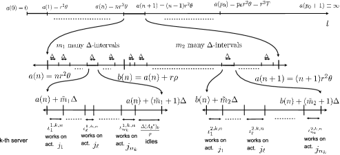
Figure 4: The figure above shows the behavior, under $T^{(1)}$, of the $k$th server, that is, responsible for the $n_{k}$ activities ($j_{1},\ldots,j_{n_{k}}$). The actual policy $T$ is given as a certain modification of $T^{(1)}$ that ensures feasibility and a strict positivity property.

The policy $T\equiv T^{r}$ is constructed recursively over time intervals $\mathcal{I}(n),n=0,\ldots,p_{0}$, as follows. We will describe the effect of the policy on the $k$th server (for each $k\in\mathbb{K}$) at every time-instant $s\geq 0$ (see Figure 4). Recall the set $\mathbb{J}(k)$ introduced in Section 2. Let for $k\in\mathbb{K}$, $j_{1}<j_{2}<\cdots<j_{n_{k}}$ be the ordered elements of $\mathbb{J}(k)$ (the set of activities that the $k$th server can perform).

Step 1: [$T^{r}(s)$ when $s\in\mathcal{I}(0)$]. Let $m_{0}=\lfloor\frac{r^{2}\theta}{\Delta}\rfloor$. Recall that $\tilde{Y}(0)=\varepsilon_{0}y^{*}$. Write $\nu^{0}=\varepsilon_{0}y^{*}$. For $k\in\mathbf{K}$, let

$$\nabla_{\ell}^{1,k,0}\doteq\biggl{(}x_{j_{\ell}}^{*}-\frac{\nu^{0}_{j_{\ell}}}{\rho}\biggr{)}\Delta,\quad\nabla_{\ell}^{2,k,0}\doteq x_{j_{\ell}}^{*}\Delta,\quad\ell=1,\ldots,n_{k}.$$ (96)

Note that, by our choice of $\rho$, $\nabla_{\ell}^{1,k,0}>0$ if $j_{l}$ is a basic activity. Also, if $j_{l}$ is nonbasic, then $x^{*}_{j_{l}}=0$, but since $K\nu^{0}\geq 0$, we have $\nu^{0}_{j_{l}}\leq 0$. Thus, $\nabla_{\ell}^{1,k,0}\geq 0$ for every $l,k$. Also, from Assumption 2.3 [see (14)] and recalling that $A\nu^{0}\geq 0$, we get

$$\sum_{l=1}^{n_{k}}\nabla_{\ell}^{1,k,0}=\Delta\biggl{(}1-\frac{1}{\rho}(A\nu^{0})_{k}\biggr{)}\leq\Delta,\quad\sum_{l=1}^{n_{k}}\nabla_{\ell}^{2,k,0}=\Delta,\quad k\in\mathbb{K}.$$ (97)

Let $m_{1}\equiv m_{1}^{r}\doteq\lfloor\frac{r\rho}{\Delta}\rfloor$ and $m_{2}\equiv m_{2}^{r}\doteq\lfloor\frac{r^{2}\theta-r\rho}{\Delta}\rfloor$. Define, for each $k\in\mathbb{K}$, and $l=1,\ldots,n_{k},$

$$\dot{T}^{(1)}_{j_{l}}(s)=\cases{\displaystyle\sum_{m=0}^{m_{1}-1}1_{\mathcal{E}_{l}^{m,0}}(s),&\quad$s\in\mathcal{I}_{1}(0),$\vspace*{2pt}\cr\displaystyle\sum_{m=0}^{m_{2}-1}1_{\hat{\mathcal{E}}_{l}^{m,0}}(s),&\quad$s\in\mathcal{I}_{2}(0),$}$$

where for $\tilde{m}_{i}=0,\ldots,m_{i}-1$, $i=1,2$, $l=1,\ldots,n_{k}$,

$$\mathcal{E}_{l}^{\tilde{m}_{1},0} = \Biggl{[}a(0)+\tilde{m}_{1}\Delta+\sum_{i=0}^{l-1}\nabla_{i}^{1,k,0},a(0)+\tilde{m}_{1}\Delta+\sum_{i=0}^{l}\nabla_{i}^{1,k,0}\Biggr{)},$$ (98)

$$\hat{\mathcal{E}}_{l}^{\tilde{m}_{2},0} = \Biggl{[}b(0)+\tilde{m}_{2}\Delta+\sum_{i=0}^{l-1}\nabla_{i}^{2,k,0},b(0)+\tilde{m}_{2}\Delta+\sum_{i=0}^{l}\nabla_{i}^{2,k,0}\Biggr{)}$$ (99)

and, by convention, $\nabla_{0}^{i,k,0}=0$, $i=1,2$. Since $\{\mathbb{J}(k),k\in\mathbb{K}\}$ gives a partition of $\mathbb{J}$, the above defines the $\mathbf{J}$-dimensional process $\dot{T}^{(1)}(s)$ for $s\in[a(0),a(1))$. We set

$$T^{(1)}(s)=\int_{0}^{s}\dot{T}^{(1)}(s)\,ds,\qquad s\in\mathcal{I}(0).$$

Next, define $\mathcal{V}(s)\equiv\mathcal{V}^{r}(s)=(Q^{r}(s),X^{r}(s),T^{r}(s))$ for $s\in\mathcal{I}(0)$ by the system of equations below:

$$Q^{r}(s) = q^{r}+X^{r}(s)+r\bigl{(}\theta_{1}^{r}s-(C-P^{\prime})\operatorname{diag}(r^{2}\theta_{2}^{r})\bar{T}^{r}(s/r^{2})\bigr{)}$$

$${}+R\bigl{(}x^{*}s-T^{r}(s)\bigr{)},$$

$$X^{r}(s) = r\hat{X}^{r}(s/r^{2}),\qquad\hat{X}^{r}\mbox{ defined by (\ref{xr-defn}), }$$

$$T^{r}_{j}(s) = \int_{[0,s]}1_{\{Q^{r}_{\sigma_{1}(j)}(u-)>0\}}1_{\{Q^{r}_{\sigma_{1}(j)}(\mathsf{p}^{r}(u))>\Theta^{r}(u)\}}\,dT^{r,(1)}_{j}(u),\qquad j\in\mathbb{J},$$

where (as introduced in Section 2), $\sigma_{1}(j)$ denotes the index of the buffer that the $j$th activity is associated with. The above construction can be interpreted as follows. The policy $T$ “attempts” to implement $T^{(1)}$ over $\mathcal{I}_{1}(0)$, unless the corresponding buffer is empty (in which case, it idles). Over $\mathcal{I}_{2}(0)$, $T$ has a similar behavior, but, in addition, it idles when the corresponding buffer does not have at least $\Theta$—many jobs at the beginning of the $\Delta$-subintervals. Processing jobs only when there is a “safety-stock” at each buffer at the beginning of the $\Delta$-subinterval ensures that with “high probability” either all the activities associated with the given buffer receive nominal time effort over the interval or all of them receive zero effort. This, in particular, makes sure that the idling processes associated with the policy are consistent with the reflection terms for the Skorohod map associated with the constraint matrix $D$ [see (116)]. This property will be exploited in the weak convergence arguments of Section 4.2 [see, e.g., arguments below (4.3)].

Let $I^{r}$ be defined by (9). By construction, $T^{r}(0)=0$, $I^{r}(0)=0$ and

$$Q^{r}(s)\geq 0,\qquad T^{r}(s)\geq 0,\qquad I^{r}(s)\geq 0$$

(101)

$$\eqntext{\mbox{for }s\in\mathcal{I}(0)\mbox{ and }T^{r},I^{r}\mbox{ are nondecreasing on }\mathcal{I}(0).}$$ (102)

This completes the construction of the policy and the associated processes on $\mathcal{I}(0)$.

Step 2: [$T^{r}(s)$ for $s\in\mathcal{I}(n)$, for $1\leq n\leq p_{0}$]. Suppose now that the process $\mathcal{V}(s)$ has been defined for $s\in[a(0),a(n))$, where $1\leq n\leq p_{0}$. We now describe the construction over the interval $\mathcal{I}(n)=[a(n),a(n+1))$. Let $\hat{\chi}^{\kappa,r}(n)=\{\hat{X}^{r}(l\kappa)\dvtx l=1,\ldots,nj_{0}\}$. Recall that $nj_{0}\kappa=n\theta$. Define

$$\bar{\nu}^{r,n}\doteq\varpi_{n}(\hat{\chi}^{\kappa,r}(n),\mathcal{U}_{n}),\qquad\nu^{r,n}\doteq\vartheta_{\varepsilon_{0}}(\hat{Q}^{r}(n\theta-),\bar{\nu}^{r,n}),$$ (103)

where, as in Section 2, $\hat{Q}^{r}(t)=Q^{r}(r^{2}t)/r$, $t\geq 0$. We will suppress $\kappa$ and $r$ from the notation and write $(\hat{\chi}^{\kappa,r}(n),\bar{\nu}^{r,n},\nu^{r,n})\equiv(\hat{\chi}(n),\bar{\nu}^{n},\nu^{n})$. For each $k\in\mathbb{K}$, define

$$\nabla_{\ell}^{1,k,n}\doteq\biggl{(}x_{j_{\ell}}^{*}-\frac{\nu^{n}_{j_{\ell}}}{\rho}\biggr{)}\Delta,\quad\nabla_{\ell}^{2,k,n}\doteq x_{j_{\ell}}^{*}\Delta,\quad\ell=1,\ldots,n_{k}.$$ (104)

As before, (97) (with $\nabla_{\ell}^{j,k,0}$ replaced by $\nabla_{\ell}^{j,k,n}$) is satisfied. Define, for each $k\in\mathbb{K}$, and $l=1,\ldots,n_{k},$

$$\dot{T}^{1}_{j_{l}}(s)=\cases{\displaystyle\sum_{m=0}^{m_{1}-1}1_{\mathcal{E}_{l}^{m,n}}(s),&\quad$s\in\mathcal{I}_{1}(n),$\vspace*{2pt}\cr\displaystyle\sum_{m=0}^{m_{2}-1}1_{\hat{\mathcal{E}}_{l}^{m,n}}(s),&\quad$s\in\mathcal{I}_{2}(n),$}$$ (105)

where for $\tilde{m}_{i}=0,\ldots,m_{i}-1$, $i=1,2$, $l=1,\ldots,n_{k}$, $\mathcal{E}_{l}^{\tilde{m}_{1},n},\hat{\mathcal{E}}_{l}^{\tilde{m}_{2},n}$ are defined by the right-hand side of (98) and (99) respectively, with $(a(0),b(0),\nabla_{i}^{1,k,0},\allowbreak\nabla_{i}^{2,k,0})$ replaced by $(a(n),b(n),\nabla_{i}^{1,k,n},\nabla_{i}^{2,k,n})$ We set

$$T^{1}(s)=T(a(n))+\int_{a(n)}^{s}\dot{T}^{1}(s)\,ds,\qquad s\in\mathcal{I}(n)$$

and define $\mathcal{V}(s)$ for $s\in\mathcal{I}(n)$ by the system of equations in (4.1).

The above recursive procedure gives a construction for the process $\mathcal{V}^{r}(s)=(Q^{r}(s),X^{r}(s),T^{r}(s))$ for all $s\in[0,\infty)$.

The policy constructed above clearly satisfies parts (i), (ii) and (iii) of Definition 2.7. In fact, it also satisfies part (iv) of the definition and, consequently, we have the following result. The proof is given in the Appendix.

Proposition 4.1

For all $r\geq r_{0}$, $T^{r}\in\mathcal{A}^{r}(q^{r})$.

4.2 Convergence of costs

In this section we prove Theorem 2.17 by showing that, with $\{T^{r}\}$ as in Section 4.1 and $\tilde{Y}$ as introduced above Theorem 3.8, $J^{r}(q^{r},T^{r})\to\tilde{J}(q,\tilde{Y})$, as $r\to\infty$. We begin with an elementary lemma.

Lemma 4.2

Let $g^{n}\in\mathcal{D}^{\mathbf{I}}$, $n\geq 1$, $g\in\mathcal{C}^{\mathbf{I}}$ be such that $g^{n}\to g$ u.o.c. as $n\to\infty$. Let $\varepsilon_{n}\in(0,\infty)$, $n\geq 1$, be such that $\varepsilon_{n}\to 0$ as $n\to\infty$. Let $B^{n},B$ be $\mathbf{I}\times\mathbf{I}$ matrices such that $B^{n}\to B$ as $n\to\infty$. Suppose $f^{n},h^{n}\in\mathcal{D}^{\mathbf{I}}$ and $\gamma^{n}\in\mathcal{D}^{1}$ satisfy for all $t\geq 0$: [(iii)]

$f^{n}(t)\geq 0$, $\gamma^{n}(t)\geq 0$,

$f^{n}(t)=g^{n}(t)+B^{n}h^{n}(t),h^{n}_{i}(t)=\int_{[0,t]}1_{\{f^{n}_{i}(\gamma^{n}(s))\leq\varepsilon_{n}\}}\,ds,i\in\mathbb{I}$ and

$|\gamma^{n}(t)-t|\leq\varepsilon_{n}$. Then $(f^{n},g^{n},h^{n},\gamma^{n})$ is precompact in $\mathcal{D}^{3\mathbf{I}+1}$ and any limit point $(f,g,h,\gamma)$ satisfies for all $t\geq 0$, $\gamma(t)=t$; $f(t)=g(t)+Bh(t)$; $h(t)=\int_{[0,t]}\tilde{h}(s)\,ds$, where $\tilde{h}\dvtx[0,\infty)\to[0,1]^{\mathbf{I}}$ is a measurable map such that

$$\int_{[0,t]}1_{\{f_{i}(s)>0\}}\tilde{h}_{i}(s)\,ds=0\qquad\mbox{for all }t\geq 0.$$

The proof of the above lemma is given in the Appendix. Recall the definitions of various scaled processes given in (2)–(25), and that $\mathpzc{i}(t)=t$ for $t\geq 0$. In addition, we define $\bar{T}^{r,1}(t)=T^{r,1}(r^{2}t)/r^{2}$, $\hat{T}^{r,1}(t)=T^{r,1}(r^{2}t)/r$, $r>0$, $t\geq 0$.

Proposition 4.3

As $r\to\infty$, $\bar{T}^{r}\to x^{*}\mathpzc{i}$, u.o.c. in probability.

From the definition of $T^{r,1}$ [see (105)], and the observation that the interval $\hat{\mathcal{E}}_{l}^{m,n}$ has length $x^{*}_{j_{l}}\Delta$ [see (97) and (99)], we have that over each interval $[m\Delta,(m+1)\Delta)$, that is, contained in $\mathcal{I}_{2}(n)$ for some $n\leq p_{0}$, the Lebesgue measure of the time instants $s$ such that $\dot{T}_{j}^{1}(s)=1$ equals $x^{*}_{j}\Delta$, $j\in\mathbb{J}$. This is equivalent to the statement that

$$\int_{[m\Delta,(m+1)\Delta)}d\bigl{(}T^{r,1}_{j}(s)-x^{*}_{j}s\bigr{)}=0$$

(106)

$$\eqntext{\mbox{whenever }\bigl{[}m\Delta,(m+1)\Delta\bigr{)}\subset\mathcal{I}_{2}(n)\mbox{ for some }n\leq p_{0}.}$$ (107)

Also, noting that for $j\in\mathbb{J}$, $0\leq\dot{T}^{r,1}_{j}\leq 1$ and $x^{*}_{j}\leq 1$, we have that for some $C_{1}>0$,

$$\int_{[m\Delta,(m+1)\Delta)}d\bigl{(}T^{r,(1)}_{j}(s)+x^{*}_{j}s\bigr{)}<C_{1}\Delta$$

(108)

$$\eqntext{\mbox{whenever }\bigl{[}m\Delta,(m+1)\Delta\bigr{)}\subset\mathcal{I}(n)\mbox{ for some }n\leq p_{0}.}$$ (109)

Fix $j\in\mathbb{J}$ and $t>0$ such that $r^{2}t\in[a(n),a(n+1))$ for some $n\leq p_{0}$. Then

$$r^{2}|x^{*}_{j}t-\bar{T}^{r,1}_{j}(t)|$$

$$\qquad\leq\sum_{n_{0}=0}^{n}\sum_{\ell=1}^{2}\sum_{m\dvtx[m\Delta,(m+1)\Delta)\in\mathcal{I}_{\ell}(n_{0})}\int_{[m\Delta\wedge t,(m+1)\Delta\wedge t)}d\bigl{(}T^{r,1}_{j}(s)-x^{*}_{j}s\bigr{)}.$$

Using (4.2) and (4.2) and the fact that the number of $\Delta$ intervals in $\mathcal{I}_{1}(n)$ is bounded by $r\rho/\Delta$, we see that

$$r^{2}|x_{j}^{*}t-\bar{T}^{r,1}_{j}(t)|\leq\biggl{(}\frac{r\rho(p_{0}+1)}{\Delta}+1\biggr{)}C_{1}\Delta.$$

Thus, for some $\varrho\in(0,\infty)$,

$$\sup_{0\leq t<\infty}|x^{*}t-\bar{T}^{r,1}(t)|\leq\varrho/r\qquad\mbox{for all }r\geq r_{0}.$$ (110)

Also, since $\bar{T}^{r}_{j}(t)\leq t$ for all $t\geq 0$, $j\in\mathbb{J}$, we get from (2) and standard estimates for renewal processes (see, e.g., Lemma 3.5 of BudGho2 ) that $\bar{X}^{r}\doteq\hat{X}^{r}/r$ converges to $0$ u.o.c. in probability, as $r\to\infty$. Combining this with Assumption 2.3 and (110), we have

$$\bar{\zeta}^{r}\doteq\hat{\zeta}^{r}/r\mbox{ converges to }0,\mbox{ u.o.c., in probability. }$$ (111)

Next, define $\bar{\mathsf{p}}^{r}(s)=\mathsf{p}^{r}(r^{2}s)/r^{2}$, $\bar{\Theta}^{r}(s)=\Theta^{r}(r^{2}s)/r^{2}$ and

$$\mathcal{S}_{j}^{r}(t) = \bigl{\{}s\in[0,t]\dvtx\bar{Q}^{r}_{\sigma_{1}(j)}(s)=0,\mbox{or }\bar{Q}^{r}_{\sigma_{1}(j)}(\bar{\mathsf{p}}^{r}(s))\leq\bar{\Theta}^{r}(s)\bigr{\}}$$

$$= \bigl{\{}s\in[0,t]\dvtx\bar{Q}^{r}_{\sigma_{1}(j)}(\bar{\mathsf{p}}^{r}(s))\leq\bar{\Theta}^{r}(s)\bigr{\}}$$

$${}\cup\bigl{\{}s\in[0,t]\dvtx\bar{Q}^{r}_{\sigma_{1}(j)}(s)=0,\bar{Q}^{r}_{\sigma_{1}(j)}(\bar{\mathsf{p}}^{r}(s))>\bar{\Theta}^{r}(s)\bigr{\}}$$

$$\doteq \mathcal{S}_{j}^{r,1}(t)\cup\mathcal{S}_{j}^{r,2}(t).$$

We will fix $t>0$ for the rest of the proof and suppress $t$ from the notation when writing $\mathcal{S}_{j}^{r,i}(t)$, unless there is scope for confusion. Using the above display and (4.1), we have that

$$\bar{T}^{r,1}_{j}(t)-\bar{T}^{r}_{j}(t)=\int_{[0,t]}1_{\mathcal{S}_{j}^{r}}(s)\,d\bar{T}^{r,1}_{j}(s),\qquad j\in\mathbb{J},t\geq 0.$$ (113)

Using the fact that $\bar{Q}^{r}(\cdot)=\frac{\hat{Q}^{r}(\cdot)}{r}$ along with (24) and (113), we can write

$$\bar{Q}^{r}(t)=\bar{\zeta}^{r}(t)+R\bar{H}^{r}(t)+R\bar{L}^{r}(t),\qquad t\geq 0,$$ (114)

where for $j\in\mathbb{J}$,

$$\bar{H}^{r}_{j}(t) = \bigl{(}x^{*}_{j}t-\bar{T}^{r,1}(t)\bigr{)}+\int_{[0,t]}1_{\mathcal{S}_{j}^{r,1}}(s)\,d\bigl{(}\bar{T}^{r,1}_{j}(s)-x^{*}_{j}s\bigr{)}$$

$${}+\int_{[0,t]}1_{\mathcal{S}_{j}^{r,2}}(s)\,d\bar{T}^{r,1}_{j}(s)$$

and

$$\bar{L}^{r}_{j}(t)=x^{*}_{j}\int_{[0,t]}1_{\mathcal{S}_{j}^{r,1}}(s)\,ds=(\operatorname{diag}(x^{*})C^{\prime}\bar{\ell}^{r})_{j}(t),$$

where

$$\bar{\ell}^{r}_{i}(t)=\int_{[0,t]}1_{\{\bar{Q}^{r}_{i}(\bar{\mathsf{p}}^{r}(s))\leq\bar{\Theta}^{r}(s)\}}\,ds,\qquad t\geq 0,i\in\mathbb{I}.$$

Since $D=R\operatorname{diag}(x^{*})C^{\prime}$ [see (11) and (43)], we have

$$\bar{Q}^{r}=\bar{\zeta}^{r}+R\bar{H}^{r}+D\bar{\ell}^{r}.$$ (116)

Next, letting $\hat{m}_{0}^{r}=\lfloor\frac{r^{2}t}{\Delta^{r}}\rfloor+1$, we have from the choice of $d_{1}$ [see above (95)] that

$$\mathbb{P}(\mathcal{S}_{j}^{r,2}\neq\varnothing)$$

$$\qquad\leq\sum_{k=0}^{\hat{m}_{0}^{r}}\sum_{i\in\mathbb{I}}\mathbb{P}\bigl{(}Q_{i}^{r}(k\Delta^{r})>d_{1}r^{\bolds{\mathsf{k}}},Q_{i}^{r}(u)=0$$

$$\qquad\qquad\mbox{ for some }u\in\bigl{[}k\Delta^{r},(k+1)\Delta^{r}\bigr{)}\bigr{)}$$

$$\qquad\leq\mathbf{I}\sum_{k=0}^{\hat{m}_{0}^{r}}\sum_{j\in\mathbb{J}}\mathbb{P}\bigl{(}S_{j}^{r}\bigl{(}T_{j}^{r}(k\Delta^{r})+\Delta^{r}\bigr{)}-S_{j}^{r}(T_{j}^{r}(k\Delta^{r}))\geq d_{1}r^{\bolds{\mathsf{k}}}\bigr{)}$$ (117)

$$\qquad\leq{\hat{m}_{0}^{r}}\mathbf{I}\mathbf{J}\frac{\varsigma(1)}{r^{\bolds{\mathsf{k}}\bolds{\mathsf{m}}}}$$

$$\qquad\leq C_{2}(t+1)r^{2-\bolds{\mathsf{k}}(1+\bolds{\mathsf{m}})},$$

for some $C_{2}\in(0,\infty)$, where the next to last inequality makes use of Assumption 2.13. Recalling [from (94)] that $\upsilon=\bolds{\mathsf{k}}(1+\bolds{\mathsf{m}})-2>1$, we get that

$$\mathbb{P}(\mathcal{S}_{j}^{r,2}\neq\varnothing)\leq C_{2}(t+1)r^{-\upsilon}\to 0\qquad\mbox{as }r\to\infty.$$ (118)

We note that the above convergence only requires that $\upsilon>0$. The property $\upsilon>1$ will, however, be needed in the proof of Proposition 4.4 [see (4.2)]. Next, using (4.2) and (4.2), we have for some $\varrho_{1}\in(0,\infty)$,

$$\sup_{0\leq u<\infty}\biggl{|}\int_{[0,u]}1_{\mathcal{S}_{j}^{r,1}}\,d\bigl{(}\bar{T}^{r,1}_{j}(s)-x^{*}_{j}s\bigr{)}\biggr{|}\leq\frac{\varrho_{1}}{r}\to 0\qquad\mbox{as }r\to\infty,$$ (119)

for all $j\in\mathbb{J}$. The above inequality follows from the fact that the integral can be written as the sum of integrals over $\Delta$-subintervals: When the subinterval is within some $\mathcal{I}_{2}(n)$, the integral is zero [using the definition of $\mathsf{p}^{r}(s)$ in such intervals and (4.2)] and when the subinterval is within some $\mathcal{I}_{1}(n)$ [the number of such intervals is $(p_{0}+1)m_{1}^{r}$ which can be bounded by $C_{3}\frac{r\rho}{\Delta}$ for some $C_{3}$], the integral is bounded by $C_{1}\Delta/r^{2}$ from (4.2).

Now, combining (110), (118) and (119), we have that, for each $j\in\mathbb{J}$, $\bar{H}^{r}_{j}\to 0$, u.o.c. in probability, as $r\to\infty$. From (116), (111), Lemma 4.2 and unique solvability of the Skorohod problem for $(0,D)$, we now have that $(\bar{Q}^{r},\bar{\ell}^{r})\to(0,0)$, u.o.c. in probability, as $r\to\infty$. Thus, $\bar{L}^{r}$ converges to $0$ as well. The result now follows on noting that $\bar{T}^{r}=x^{*}\mathpzc{i}-\bar{H}^{r}-\bar{L}^{r}$.

The following proposition gives a key estimate in the proof of Theorem 2.17.

Proposition 4.4

For some $c_{2}\in(0,\infty)$ and $\bar{\upsilon}\in(1,\infty)$,

$$\mathbb{E}(|\hat{Q}^{r}|^{\bar{\upsilon}}_{\infty,t}+|\hat{\zeta}^{r}|^{\bar{\upsilon}}_{\infty,t}+|\hat{Y}^{r}|^{\bar{\upsilon}}_{\infty,t})\leq c_{2}(1+t^{3})\qquad\mbox{for all }r\geq r_{0},t\geq 0.$$

Using standard moment estimates for renewal processes (cf. Lemma 3.5 of BudGho2 ), one can find $C_{1}\in(0,\infty)$ such that

$$\mathbb{E}|\hat{\zeta}^{r}|^{2}_{\infty,t}\leq C_{1}(1+t^{2})\qquad\mbox{for all }r\geq r_{0},t\geq 0.$$ (120)

From (114) and (116), we have

$$\hat{Q}^{r}(t)=\hat{\zeta}^{r}(t)+R\hat{H}^{r}(t)+R\hat{L}^{r}(t)=\hat{\zeta}^{r}(t)+R\hat{H}^{r}(t)+D\hat{\ell}^{r}(t),\qquad t\geq 0,$$

where $\hat{H}^{r}=r\bar{H}^{r}$, $\hat{L}^{r}=r\bar{L}^{r}$ and $\hat{\ell}^{r}=r\bar{\ell}^{r}$. We rewrite the above display as

$$\hat{Q}^{r}(\bar{\mathsf{p}}^{r}(t))=[\hat{Q}^{r}(\bar{\mathsf{p}}^{r}(t))-\hat{Q}^{r}(t)]+\hat{\zeta}^{r}(t)+R\hat{H}^{r}(t)+D\hat{\ell}^{r}(t),\qquad t\geq 0.$$

From Theorem 5.1 of will-invpr , for some $C_{2}\in(0,\infty)$,

$$|\hat{\ell}^{r}|_{\infty,t}+|\hat{Q}^{r}|_{\infty,t}$$

$$\qquad\leq C_{2}\biggl{(}\hat{q}^{r}+|\hat{\zeta}^{r}|_{\infty,t}+|\hat{H}^{r}|_{\infty,t}+|\hat{Q}^{r}(\bar{\mathsf{p}}^{r}(\cdot))-\hat{Q}^{r}|_{\infty,t}+\frac{d_{1}r^{\bolds{\mathsf{k}}}}{r}\biggr{)}.$$

Also, from (4.2), (110) and (119), for all $t\geq 0$ and $r\geq r_{0}$,

$$\biggl{|}\hat{H}^{r}_{j}(t)-r\int_{[0,t]}1_{\mathcal{S}_{j}^{r,2}}(s)\,d\bar{T}^{r,1}_{j}(s)\biggr{|}\leq\varrho+\varrho_{1}.$$ (122)

Next, using (118), we get, for some $C_{3}\in(0,\infty)$,

$$\mathbb{E}\biggl{(}r\sup_{0\leq u\leq t}\int_{[0,u]}1_{\mathcal{S}_{j}^{r,2}}(s)\,d\bar{T}^{r,1}_{j}(s)\biggr{)}^{\upsilon\wedge 2} \leq r^{\upsilon}C_{3}(t^{3}+1)r^{-\upsilon}$$

$$\leq C_{3}(t^{3}+1).$$

Finally, for some $C_{4}\in(1,\infty)$, for all $a\geq 1$,

$$\mathbb{P}\bigl{(}|\hat{Q}^{r}(\bar{\mathsf{p}}^{r}(\cdot))-\hat{Q}^{r}(\cdot)|_{\infty,t}\geq a\bigr{)}$$

(124)

$$\qquad\leq\frac{r^{2}t}{\Delta^{r}}\biggl{(}\sum_{i\in\mathbb{I}}\mathbb{P}\biggl{(}A_{i}^{r}(\Delta^{r})\geq\frac{ar}{C_{4}}\biggr{)}+\sum_{j\in\mathbb{J}}\mathbb{P}\biggl{(}S_{j}^{r}(\Delta^{r})\geq\frac{ar}{C_{4}}\biggr{)}\biggr{)}.$$

Using moment estimates for renewal process once more (Lemma 3.5 of BudGho2 ), we can find $C_{5}\in(0,\infty)$ such that

$$\mathbb{P}\bigl{(}|\hat{Q}^{r}(\bar{\mathsf{p}}^{r}(\cdot))-\hat{Q}^{r}(\cdot)|_{\infty,t}\geq a\bigr{)} \leq \frac{r^{2}t}{\Delta^{r}}\frac{C_{5}\Delta^{r}}{(ar-C_{5}\Delta^{r})^{2}}$$

$$\leq \frac{1}{a^{2}}\frac{C_{5}r^{2}t}{(r-{C_{5}\Delta^{r}}/{a})^{2}}.$$

Thus, there is an $r_{1}\in(r_{0},\infty)$ and $C_{6}\in(0,\infty)$ such that, for all $r\geq r_{1}$,

$$\mathbb{P}\bigl{(}|\hat{Q}^{r}(\bar{\mathsf{p}}^{r}(\cdot))-\hat{Q}^{r}(\cdot)|_{\infty,t}\geq a\bigr{)}\leq\frac{1}{a^{2}}C_{6}(t+1).$$ (125)

This shows that for some $\upsilon_{1}\in(1,\infty)$ and $C_{7}\in(0,\infty)$,

$$\mathbb{E}|\hat{Q}^{r}(\bar{\mathsf{p}}^{r}(\cdot))-\hat{Q}^{r}(\cdot)|^{\upsilon_{1}}_{\infty,t}\leq C_{7}(1+t),\qquad t\geq 0.$$ (126)

The result now follows on using (120), (122), (4.2) and (126) in (4.2) and observing that $\hat{Y}^{r}=\hat{H}^{r}+\operatorname{diag}(x^{*})C^{\prime}\hat{\ell}^{r}$.

In preparation for the proof of Theorem 2.17, we introduce the following notation. For $n=0,\ldots,p_{0}-1$, we define processes $\mathbf{\mathpzc{q}}^{r,n},\mathbf{\mathpzc{z}}^{r,n}$ with paths in $\mathcal{D}^{\mathbf{I}}_{\theta}$ and $\mathcal{C}^{\mathbf{J}}_{\theta}$, respectively, as

$$(\mathbf{\mathpzc{q}}^{r,n}(t),\mathbf{\mathpzc{z}}^{r,n}(t))=\cases{\bigl{(}\hat{Q}^{r}(n\theta+\rho/r),0\bigr{)},&\quad$t\in[0,\rho/r),$\vspace*{2pt}\cr\bigl{(}\hat{Q}^{r}(t+n\theta),\hat{Y}^{r}(t+n\theta)-\hat{Y}^{r}(n\theta+\rho/r)\bigr{)},&\quad$t\in[\rho/r,\theta].$}$$

We denote by $\mathbf{\mathpzc{q}}^{r,p_{0}},\mathbf{\mathpzc{z}}^{r,p_{0}}$ the processes with paths in $\mathcal{D}^{\mathbf{I}}$ and $\mathcal{C}^{\mathbf{J}}$, respectively, defined by the right-hand side in the display above, by replacing $n$ by $p_{0}$ and $[\rho/r,\theta]$ with $[\rho/r,\infty)$. Then

$$\mathbf{\mathpzc{q}}^{r}\doteq(\mathbf{\mathpzc{q}}^{r,*},\mathbf{\mathpzc{q}}^{r,p_{0}})\in\mathcal{D}_{\theta}^{p_{0}\mathbf{I}}\times\mathcal{D}^{\mathbf{I}}\qquad\mbox{a.s.},$$

where $\mathbf{\mathpzc{q}}^{r,*}=(\mathbf{\mathpzc{q}}^{r,0},\ldots,\mathbf{\mathpzc{q}}^{r,p_{0}-1})$. Similarly, define the process $\mathbf{\mathpzc{z}}^{r}$ with paths in $\mathcal{C}_{\theta}^{p_{0}\mathbf{J}}\times\mathcal{C}^{\mathbf{J}}$. Recall $\bar{\nu}^{r,n},\nu^{r,n}$ introduced in (103). Denote $\bar{\nu}^{r}=(\bar{\nu}^{r,0},\bar{\nu}^{r,1},\ldots,\allowbreak\bar{\nu}^{r,p_{0}})$ and $\nu^{r}=(\nu^{r,0},\nu^{r,1},\ldots,\nu^{r,p_{0}})$, where we set $\bar{\nu}^{r,0}=0$ and $\nu^{r,0}=\varepsilon_{0}y^{*}$.

Next, for $n=0,\ldots,p_{0}-1$, define processes $\mathbf{\mathpzc{q}}^{(n)},\mathbf{\mathpzc{z}}^{(n)}$ with paths in $\mathcal{C}^{\mathbf{I}}_{\theta}$ and $\mathcal{C}^{\mathbf{J}}_{\theta}$, respectively, as

$$\bigl{(}\mathbf{\mathpzc{q}}^{(n)}(t),\mathbf{\mathpzc{z}}^{(n)}(t)\bigr{)}=\cases{\bigl{(}\tilde{Q}(t+n\theta),\tilde{Y}(t+n\theta)-\tilde{Y}(n\theta)\bigr{)},&\quad$t\in[0,\theta),$\vspace*{2pt}\cr\bigl{(}\tilde{Q}\bigl{(}(n+1)\theta-\bigr{)},\tilde{Y}\bigl{(}(n+1)\theta-\bigr{)}-\tilde{Y}(n\theta)\bigr{)},&\quad$t=\theta.$}$$

Also, define $\mathbf{\mathpzc{q}}^{(p_{0})},\mathbf{\mathpzc{z}}^{(p_{0})}$ by the first line of the above display by replacing $\theta$ by $\infty$. Then $\mathbf{\mathpzc{q}}\doteq(\mathbf{\mathpzc{q}}^{*},\mathbf{\mathpzc{q}}^{(p_{0})})\in\mathcal{C}_{\theta}^{p_{0}\mathbf{I}}\times\mathcal{C}^{\mathbf{I}}$, a.s., where $\mathbf{\mathpzc{q}}^{*}=(\mathbf{\mathpzc{q}}^{(0)},\ldots,\mathbf{\mathpzc{q}}^{(p_{0}-1)})$. Similarly, define the process $\mathbf{\mathpzc{z}}$ with paths in $\mathcal{C}_{\theta}^{p_{0}\mathbf{J}}\times\mathcal{C}^{\mathbf{J}}$. Also, let for $n=1,\ldots,p_{0}$, $\bar{\nu}^{(n)}=\partial\tilde{Y}_{0}^{(1)}(n)=\tilde{Y}_{0}^{(1)}(n\theta)-\tilde{Y}_{0}^{(1)}((n-1)\theta)$, where $\tilde{Y}_{0}^{(1)}$ is as above (60), and $\nu^{(n)}=\tilde{Y}(n\theta)-\tilde{Y}(n\theta-)$. Then

$$\bar{\nu}^{(n)}\doteq\varpi_{n}(\chi^{\kappa}(n),\tilde{\mathcal{U}}_{n}),\qquad\nu^{(n)}\doteq\vartheta_{\varepsilon_{0}}\bigl{(}\tilde{Q}(n\theta-),\bar{\nu}^{(n)}\bigr{)}.$$ (127)

Define $\bar{\nu}=(\bar{\nu}^{(0)},\bar{\nu}^{(1)},\ldots,\bar{\nu}^{(p_{0})})$ and $\nu=(\nu^{(0)},\nu^{(1)},\ldots,\nu^{(p_{0})})$, where $\bar{\nu}^{(0)}=0$ and $\nu^{(0)}=\varepsilon_{0}y^{*}$. Then $\bar{\nu}^{r},\bar{\nu}\in(\mathcal{S}_{M}^{\eta})^{\otimes(p_{0}+1)}$ and $\nu^{r},\nu\in\mathbb{R}^{\mathbf{J}(p_{0}+1)}$. Next, let

$$\nu_{0}^{r,n}=\hat{Y}^{r}(n\theta+\rho/r),\qquad\nu_{0}^{(n)}=\tilde{Y}(n\theta),\qquad n=0,1,\ldots,p_{0}.$$

Then $\nu_{0}^{r}\doteq(\nu_{0}^{r,0},\ldots,\nu_{0}^{r,p_{0}});\nu_{0}\doteq(\nu_{0}^{(0)},\ldots,\nu_{0}^{(p_{0})})\in\mathbb{R}^{\mathbf{J}(p_{0}+1)}.$ Let

$$\Xi=\mathcal{D}^{\mathbf{I}}\times(\mathcal{S}_{M}^{\eta})^{\otimes(p_{0}+1)}\times\bigl{(}\mathbb{R}^{\mathbf{J}(p_{0}+1)}\bigr{)}\times\bigl{(}\mathbb{R}^{\mathbf{J}(p_{0}+1)}\bigr{)}\times(\mathcal{D}_{\theta}^{p_{0}\mathbf{I}}\times\mathcal{D}^{\mathbf{I}})\times(\mathcal{C}_{\theta}^{p_{0}\mathbf{J}}\times\mathcal{C}^{\mathbf{J}}).$$

Note that $\mathcal{J}^{r}\doteq(\hat{\zeta}^{r},\bar{\nu}^{r},\nu^{r},\nu_{0}^{r},\mathbf{\mathpzc{q}}^{r},\mathbf{\mathpzc{z}}^{r})$, $r\geq 1$ and $\mathcal{J}=(\tilde{\zeta},\bar{\nu},\nu,\nu_{0},\mathbf{\mathpzc{q}},\mathbf{\mathpzc{z}})$ are $\Xi$-valued random variables. The following is the main step in the proof of Theorem 2.17.

Theorem 4.5

As $r\to\infty$, $\mathcal{J}^{r}\Rightarrow\mathcal{J}.$

Proof of the above theorem is given in the next subsection. Using Theorem 4.5, the proof of Theorem 2.17 is now completed as follows.

Proof of Theorem 2.17 From proposition and integration by parts,

$$J^{r}(q^{r},T^{r}) = \sum_{n=0}^{p_{0}}\biggl{[}\mathbb{E}\int_{[b^{r}(n)/r^{2},a^{r}(n+1)/r^{2})}e^{-\gamma t}\bigl{(}h\cdot\hat{Q}^{r}(t)+\gamma p\cdot\hat{U}^{r}(t)\bigr{)}\,dt$$

$$\hskip 18.0pt{}+\mathbb{E}\int_{[a^{r}(n)/r^{2},b^{r}(n)/r^{2})}e^{-\gamma t}\bigl{(}h\cdot\hat{Q}^{r}(t)+\gamma p\cdot\hat{U}^{r}(t)\bigr{)}\,dt\biggr{]}$$

$$= \sum_{n=0}^{p_{0}}\mathbb{E}\int_{[b^{r}(n)/r^{2},a^{r}(n+1)/r^{2})}e^{-\gamma t}\bigl{(}h\cdot\hat{Q}^{r}(t)+\gamma p\cdot\hat{U}^{r}(t)\bigr{)}\,dt+\varepsilon_{r},$$

where, using Proposition 4.4 and the observation that $a^{r}(n+1)/r^{2}-b^{r}(n)/\allowbreak r^{2}\leq\rho/r\to 0$, we have that $\varepsilon_{r}\to 0$ as $r\to\infty$. From Theorem 4.5, as $r\to\infty$, $\mathbf{\mathpzc{q}}^{r}\Rightarrow\mathbf{\mathpzc{q}}$. Combining this with Proposition 4.4, we get for every $n=0,\ldots,p_{0}$,

$$\lim_{r\to\infty}\mathbb{E}\int_{[b^{r}(n)/r^{2},a^{r}(n+1)/r^{2})}e^{-\gamma t}h\cdot\hat{Q}^{r}(t)\,dt$$

$$\qquad=\lim_{r\to\infty}\mathbb{E}\int_{[n\theta+\rho/r,(n+1)\theta)}e^{-\gamma t}h\cdot\hat{Q}^{r}(t)\,dt$$

$$\qquad=\lim_{r\to\infty}\mathbb{E}\int_{[n\theta,(n+1)\theta)}e^{-\gamma t}h\cdot\mathbf{\mathpzc{q}}^{r,n}(t-n\theta)\,dt$$ (129)

$$\qquad=\mathbb{E}\int_{[n\theta,(n+1)\theta)}e^{-\gamma t}h\cdot\mathbf{\mathpzc{q}}^{(n)}(t-n\theta)\,dt$$

$$\qquad=\mathbb{E}\int_{[n\theta,(n+1)\theta)}e^{-\gamma t}h\cdot\tilde{Q}(t)\,dt,$$

where, by convention, $[n\theta,(n+1)\theta)=[p_{0}\theta,\infty)$ when $n=p_{0}$. Next, for $t\in[n\theta+\rho/r,(n+1)\theta)$, $n=0,\ldots,p_{0}$,

$$\qquad\gamma p\cdot\hat{U}^{r}(t) = \gamma p\cdot K\bigl{(}\hat{Y}^{r}(t)-\hat{Y}^{r}(n\theta+\rho/r)\bigr{)}+\gamma p\cdot K\hat{Y}^{r}(n\theta+\rho/r)$$

$$= \gamma p\cdot K\mathbf{\mathpzc{z}}^{r,n}(t-n\theta)+\gamma p\cdot K\nu_{0}^{r,n}.$$

From Theorem 4.5, as $r\to\infty$,

$$\gamma p\cdot K\mathbf{\mathpzc{z}}^{r,n}(\cdot)+\gamma p\cdot K\nu_{0}^{r,n}\Rightarrow\gamma p\cdot K\mathbf{\mathpzc{z}}^{(n)}(\cdot)+\gamma p\cdot K\nu_{0}^{(n)}$$

in $\mathcal{C}_{\theta}^{1}$. Combining this with (4.2) and Proposition 4.4 we now get similarly to (4.2), for $n=0,\ldots,p_{0}$,

$$\lim_{r\to\infty} \mathbb{E}\int_{[b^{r}(n)/r^{2},a^{r}(n+1)/r^{2})}\gamma e^{-\gamma t}p\cdot\hat{U}^{r}(t)\,dt$$

$$\qquad=\lim_{r\to\infty}E\int_{[n\theta,(n+1)\theta)}\gamma e^{-\gamma t}p\cdot K\bigl{(}\mathbf{\mathpzc{z}}^{r,n}(t-n\theta)+\nu_{0}^{r,n}\bigr{)}\,dt$$

$$\qquad=E\int_{[n\theta,(n+1)\theta)}\gamma e^{-\gamma t}p\cdot K\bigl{(}\mathbf{\mathpzc{z}}^{(n)}(t-n\theta)+\nu_{0}^{(n)}\bigr{)}\,dt.$$

Note that for $t\in[n\theta,(n+1)\theta)$,

$$\mathbf{\mathpzc{z}}^{(n)}(t-n\theta)+\nu_{0}^{(n)}=\tilde{Y}(n\theta)+\tilde{Y}(t)-\tilde{Y}(n\theta)=\tilde{Y}(t).$$

Thus, the expression on the right-hand side of the above display equals

$$\mathbb{E}\int_{[n\theta,(n+1)\theta)}\gamma e^{-\gamma t}p\cdot\tilde{U}(t)\,dt.$$

The result now follows on using this observation along with (4.2) in (4.2).

4.3 Proof of Theorem 4.5

For $j\in\mathbb{J}$, $n=0,1,\ldots,p_{0}$, and $\omega\in\Omega$, define

$$\check{S}_{j}^{r,n}(\omega)=\{s\in[0,\rho]\dvtx Q^{r}_{\sigma_{1}(j)}(nr^{2}\theta+rs,\omega)=0\}.$$ (131)

From the definition of $\vartheta_{\varepsilon_{0}}$, it follows that for some $\gamma_{0}>0$,

$$\inf_{r\geq r_{0}}\min_{n=0,\ldots,p_{0};j\in\mathbb{J}}(R\nu^{r,n})_{j}\geq\gamma_{0}\qquad\mbox{a.e.}$$

As a consequence of this observation, we have the following result. The proof is given in Section 4.4.

Proposition 4.6

For some $\{\rho_{r}\}\subset[0,\rho]$ such that $\rho_{r}\to 0$ as $r\to\infty$, we have

$$\mathbb{P}(\Psi^{r}_{n})\to 1\qquad\mbox{as }r\to\infty,\mbox{ for all }n=0,1,\ldots,p_{0},$$ (132)

where $\Psi^{r}_{n}=\{\omega\in\Omega\dvtx(\bigcup_{j\in\mathbb{J}}\check{S}_{j}^{r,n}(\omega))\cap[\rho_{r},\rho]=\varnothing\}$.

For $n=0,1,\ldots,p_{0}$, let $\bar{\nu}^{r}[n]=(\bar{\nu}^{r,0},\ldots,\bar{\nu}^{r,n})$. We define $\nu^{r}[n],\nu_{0}^{r}[n],\mathbf{\mathpzc{q}}^{r}[n],\allowbreak\mathbf{\mathpzc{z}}^{r}[n]$ and their limiting analogues $\bar{\nu}[n],\nu[n],\nu_{0}[n],\mathbf{\mathpzc{q}}[n],\mathbf{\mathpzc{z}}[n]$ in a similar fashion. Set

$$\mathcal{J}^{r}[n] = (\hat{\zeta}^{r},\bar{\nu}^{r}[n],\nu^{r}[n],\nu_{0}^{r}[n],\mathbf{\mathpzc{q}}^{r}[n],\mathbf{\mathpzc{z}}^{r}[n]),$$

$$\mathcal{J}[n] = (\hat{\zeta},\bar{\nu}[n],\nu[n],\nu_{0}[n],\mathbf{\mathpzc{q}}[n],\mathbf{\mathpzc{z}}[n]).$$

Then $\mathcal{J}^{r}[n],\mathcal{J}[n]$ are $\Xi[n]$-valued random variables, with

$$\Xi[n]=\mathcal{D}^{\mathbf{I}}\times(\mathcal{S}_{M}^{\eta})^{\otimes(n+1)}\times\bigl{(}\mathbb{R}^{\mathbf{J}(n+1)}\bigr{)}\times\bigl{(}\mathbb{R}^{\mathbf{J}(n+1)}\bigr{)}\times\mathcal{D}_{\theta}^{(n+1)\mathbf{I}}\times\mathcal{C}_{\theta}^{(n+1)\mathbf{J}},$$

where we follow the usual convention for $n=p_{0}$. To prove the theorem, we need to show that $\mathcal{J}^{r}[p_{0}]\Rightarrow\mathcal{J}[p_{0}]$. In the lemma below we will in fact show, recursively in $n$, that $\mathcal{J}^{r}[n]\Rightarrow\mathcal{J}[n]$ as $r\to\infty$, for each $n=0,1,\ldots,p_{0}$, which will complete the proof of Theorem 4.5.

Lemma 4.7

For each $n=0,1,\ldots,p_{0}$, $\mathcal{J}^{r}[n]\Rightarrow\mathcal{J}[n]$, as $r\to\infty$.

The proof will follow the following two steps: [(ii)]

As $r\to\infty$, $\mathcal{J}^{r}[0]\Rightarrow\mathcal{J}[0]$.

Suppose that $\mathcal{J}^{r}[k]\Rightarrow\mathcal{J}[k]$ as $r\to\infty$ for $k=0,1,\ldots,n$, for some $n<p_{0}$. Then, as $r\to\infty$, $\mathcal{J}^{r}[n+1]\Rightarrow\mathcal{J}[n+1]$.

Consider (i). Define scaled processes $\check{Q}^{r}(t)=Q^{r}(rt)/r$, $\check{Y}^{r}(t)=Y^{r}(rt)/r$. Processes $\check{X}^{r}$, $\check{T}^{r}$, $\check{T}^{r,1}$, $\check{\zeta}^{r}$ are defined similarly. By the functional central limit theorem for renewal processes and Proposition 4.3, it follows that (cf. Lemma 3.3 of BudGho2 )

$$\hat{\zeta}^{r}\Rightarrow\tilde{\zeta}.$$ (133)

Also, convergence of $(\bar{\nu}^{r}[0],\nu^{r}[0])$ follows trivially since $\bar{\nu}^{r}[0]=\bar{\nu}[0]=0$ and $\nu^{r}[0]=\nu[0]=\varepsilon_{0}y^{*}$. Next, consider $\nu_{0}^{r}[0]=\hat{Y}^{r}(\rho/r)$. From the definition of the scaled processes defined above (131), we have that

$$\check{\zeta}^{r}(t)=\check{q}^{r}+\check{X}^{r}(t)+\frac{1}{r}[\theta_{1}^{r}t-(C-P^{\prime})\operatorname{diag}(\theta_{2}^{r})\check{T}^{r}(t)],$$ (134)

and

$$\check{Q}^{r}(t)=\check{\zeta}^{r}(t)+R\check{Y}^{r}(t),\qquad t\in[0,\rho].$$ (135)

Also, observe that $\check{Y}^{r}$ can be written as

$$\check{Y}^{r}(t)=\biggl{(}\biggl{(}x^{*}-\frac{\varepsilon_{0}y^{*}}{\rho}\biggr{)}t-\check{T}^{r,1}(t)\biggr{)}+\frac{1}{\rho}\varepsilon_{0}y^{*}t+\check{N}^{r}(t),$$ (136)

where, with $\check{S}_{j}^{r,0}$ defined in (131),

$$\check{N}_{j}^{r}(t)=\int_{[0,t]}1_{\check{S}_{j}^{r,0}}(s)\,d\check{T}^{r,1}_{j}(s).$$ (137)

Next, note that, for a suitable $C_{1}\in(0,\infty)$,

$$\biggl{|}\check{T}^{r,1}-\biggl{(}x^{*}-\frac{\varepsilon_{0}y^{*}}{\rho}\biggr{)}\mathpzc{i}\biggr{|}_{\infty,\rho}\leq C_{1}\frac{\Delta^{r}}{r}.$$ (138)

Also, $|\check{N}^{r}|_{\infty,\rho}\leq\rho_{r}+\rho 1_{(\Psi^{r}_{n})^{c}}.$ Thus, from Proposition 4.6, $|\check{N}^{r}|_{\infty,\rho}$ converges to $0$ in probability as $r\to\infty$, which shows that

$$\biggl{|}\check{Y}^{r}-\frac{\varepsilon_{0}}{\rho}y^{*}\biggr{|}_{\infty,\rho}=\biggl{|}\biggl{(}x^{*}-\frac{\varepsilon_{0}}{\rho}y^{*}\biggr{)}\mathpzc{i}-\check{T}^{r}\biggr{|}_{\infty,\rho}\to 0$$

(139)

$$\eqntext{\mbox{in probability, as }r\to\infty.}$$ (140)

The above convergence is the key reason for introducing the modification of $\tilde{Y}^{(1)}$, through the vector $y^{*}$, described above Theorem 3.8.

Next, standard moment bounds for renewal processes (see, e.g., Lemma 3.5 of BudGho2 ) yield that $|\check{X}^{r}|_{\infty,\rho}$ converges to zero in probability as $r\to\infty$. Combining these observations, we get from (134) and (135) that $(\check{Q}^{r},\check{Y}^{r})$ converge, uniformly over $[0,\rho]$, in probability, to $(q+\frac{\varepsilon_{0}}{\rho}Ry^{*}\mathpzc{i},\frac{\varepsilon_{0}y^{*}}{\rho}\mathpzc{i})$. In particular, this shows that

$$(\mathbf{\mathpzc{q}}^{r,0}(0),\nu_{0}^{r,0})=(\check{Q}^{r}(\rho),\check{Y}^{r}(\rho))$$

(141)

$$\quad\Rightarrow\quad(q+\varepsilon_{0}Ry^{*},\varepsilon_{0}y^{*})=\bigl{(}\mathbf{\mathpzc{q}}^{(0)}(0),\nu_{0}^{(0)}\bigr{)}.$$

Finally, we prove the convergence of $(\mathbf{\mathpzc{q}}^{r,0},\mathbf{\mathpzc{z}}^{r,0})$ to $(\mathbf{\mathpzc{q}}^{(0)},\mathbf{\mathpzc{z}}^{(0)})$. We will apply Theorem 4.1 of will-invpr . Note that

$$\mathbf{\mathpzc{q}}^{r,0}(t)=\mathbf{\mathpzc{q}}^{r,0}(0)+w^{r,0}(t)+R\mathbf{\mathpzc{z}}^{r,0}(t),\qquad t\in[0,\theta],$$ (142)

where $w^{r,0}$ is a $\mathcal{D}_{\theta}^{\mathbf{I}}$-valued random variable defined as $w^{r,0}(t)=(\hat{\zeta}^{r}(t)-\hat{\zeta}^{r}(\rho/r))1_{[\rho/r,\infty)}(t)$. From (4.3) and (133)

$$\mathbf{\mathpzc{q}}^{r,0}(0)\to\mathbf{\mathpzc{q}}^{(0)}(0)\quad\mbox{and}\quad w^{r,0}\Rightarrow\tilde{\zeta}\qquad\mbox{as }r\to\infty.$$ (143)

Next, for $t\in[\rho/r,\theta)$, write

$$\mathbf{\mathpzc{z}}^{r,0}(t)=\hat{H}^{r,0}(t)+\hat{L}^{r,0}(t),$$ (144)

where for $j\in\mathbb{J}$,

$$\hat{H}^{r,0}_{j}(t) = r\int_{[\rho/r,t]}\bigl{(}1-1_{\mathcal{S}_{j}^{r,1}}(s)\bigr{)}\,d\bigl{(}x^{*}_{j}s-\bar{T}^{r,1}_{j}(s)\bigr{)}+r\int_{[\rho/r,t]}1_{\mathcal{S}_{j}^{r,2}}(s)\,d\bar{T}^{r,1}_{j}(s),$$

$$\hat{L}^{r,0}_{j}(t) = rx^{*}_{j}\int_{[\rho/r,t]}1_{\mathcal{S}_{j}^{r,1}}(s)\,ds,$$

with $\mathcal{S}_{j}^{r,i}$ defined in (4.2). Using calculations similar to those in the proof of Proposition 4.3 [see (4.2)], we get

$$\sup_{\rho/r\leq t\leq\theta}\biggl{|}r\int_{[\rho/r,t]}1_{\mathcal{S}_{j}^{r,2}}(s)\bar{T}^{r,1}_{j}(s)\biggr{|}\to 0\qquad\mbox{in probability, as }r\to\infty,$$ (145)

for all $j\in\mathbb{J}$.

Also, from (4.2) it follows that

$$\sup_{\rho/r\leq t\leq\theta}\biggl{|}r\int_{[\rho/r,t]}\bigl{(}1-1_{\mathcal{S}_{j}^{r,1}}(s)\bigr{)}\,d\bigl{(}x^{*}_{j}s-\bar{T}^{r,1}_{j}(s)\bigr{)}\biggr{|}\leq\frac{\Delta^{r}}{r}.$$

Combining the above estimates,

$$\sup_{\rho/r\leq t\leq\theta}|\hat{H}_{j}^{r,0}(t)|\to 0\qquad\mbox{in probability, as }r\to\infty.$$ (146)

Also, $\hat{L}^{r,0}(t)=(\operatorname{diag}(x^{*}))C^{\prime}\hat{\ell}^{r,0}(t),$ where for $i\in\mathbb{I}$ and $t\in[\rho/r,\theta]$,

$$\hat{\ell}_{i}^{r,0}(t) = r\int_{[\rho/r,t]}1_{\{\hat{Q}^{r}_{i}(\bar{\mathsf{p}}^{r}(s))\leq r\bar{\Theta}^{r}(s)\}}\,ds$$

$$= r\int_{[\rho/r,t]}1_{\{\mathbf{\mathpzc{q}}^{r,0}_{i}(\bar{\mathsf{p}}^{r}(s))\leq r\bar{\Theta}^{r}(s)\}}\,ds.$$

Recall that $\mathbf{\mathpzc{z}}^{r,0}(t)=0$ for $t\in[0,\rho/r]$. Hence, setting $\hat{H}^{r,0}(t)=\hat{\ell}^{r,0}(t)=0$ for $t\in[0,\rho/r]$, we have from (142) and (144)

$$\qquad\mathbf{\mathpzc{q}}^{r,0}(t)=\mathbf{\mathpzc{q}}^{r,0}(0)+w^{r,0}(t)+R\hat{H}^{r,0}(t)+D\hat{\ell}^{r,0}(t),\quad t\in[0,\theta].$$ (148)

From (143) and (146) we now have that, as $r\to\infty$,

$$q^{r,0}(0)+w^{r,0}+R\hat{H}^{r,0}\Rightarrow q^{(0)}+\tilde{\zeta}$$ (149)

in $\mathcal{D}_{\theta}^{\mathbf{I}}$. Using the definition of $\mathsf{p}^{r}$, Assumption 2.13 and elementary properties of renewal processes [see similar arguments in (4.2) and (4.2)], we have that for some $C_{2}$, as $r\to\infty$,

$$\mathbb{P}\Bigl{(}\sup_{s\in[\rho/r,\theta]}|\hat{Q}^{r}(\bar{\mathsf{p}}^{r}(s))-\hat{Q}^{r}(s)|>\varepsilon\Bigr{)}\leq C_{2}\frac{r^{2}\theta}{\Delta^{r}}\frac{1}{(\Delta^{r})^{\bolds{\mathsf{m}}}}=C_{2}\frac{r^{2}\theta}{r^{\bolds{\mathsf{k}}(\bolds{\mathsf{m}}+1)}}\to 0.$$

This shows that

$$\qquad\sup_{s\in[0,\theta]}|\mathbf{\mathpzc{q}}^{r,0}(s)-\mathbf{\mathpzc{q}}^{r,0}(\bar{\mathsf{p}}^{r}(s))|\to 0\quad\mbox{in probability, as }r\to\infty.$$ (150)

Using Theorem 4.1 of will-invpr along with (4.3), (148), (149) and (150), we now have that

$$(\hat{\zeta}^{r},\mathbf{\mathpzc{q}}^{r,0},\hat{\ell}^{r,0})\Rightarrow\bigl{(}\tilde{\zeta},\Gamma\bigl{(}q^{(0)}(0)+\tilde{\zeta}\bigr{)},\hat{\Gamma}\bigl{(}q^{(0)}(0)+\tilde{\zeta}\bigr{)}\bigr{)}\qquad\mbox{as }r\to\infty,$$

as $\mathcal{D}^{\mathbf{I}}\times\mathcal{D}_{\theta}^{\mathbf{I}}\times\mathcal{D}_{\theta}^{\mathbf{I}}$ valued random variables. Since

$$\Gamma\bigl{(}q^{(0)}(0)+\tilde{\zeta}\bigr{)}=\mathbf{\mathpzc{q}}^{(0)}\quad\mbox{and}\quad\operatorname{diag}(x^{*})C^{\prime}\hat{\Gamma}\bigl{(}q^{(0)}(0)+\tilde{\zeta}\bigr{)}=\mathbf{\mathpzc{z}}^{(0)},$$

we get from the above display that $(\mathbf{\mathpzc{q}}^{r,0},\mathbf{\mathpzc{z}}^{r,0})\Rightarrow(\mathbf{\mathpzc{q}}^{(0)},\mathbf{\mathpzc{z}}^{(0)})$ as $r\rightarrow\infty$. Combining this with (4.3) and observations below (133), we have $\mathcal{J}^{r}[0]\Rightarrow\mathcal{J}[0]$, which completes the proof of (i).

We now prove (ii). We can write

$$\mathcal{J}^{r}[n+1] = (\mathcal{J}^{r}[n],(\bar{\nu}^{r,n+1},\nu^{r,n+1},\nu_{0}^{r,n+1},\mathbf{\mathpzc{q}}^{r,n+1},\mathbf{\mathpzc{z}}^{r,n+1}))$$

$$\mathcal{J}[n+1] = \bigl{(}\mathcal{J}^{r}[n],\bigl{(}\bar{\nu}^{(n+1)},\nu^{(n+1)},\nu_{0}^{(n+1)},\mathbf{\mathpzc{q}}^{(n+1)},\mathbf{\mathpzc{z}}^{(n+1)}\bigr{)}\bigr{)}.$$

By assumption,

$$\mathcal{J}^{r}[n]\Rightarrow\mathcal{J}[n]$$ (151)

and, thus, in particular, (133) holds. This shows that $\hat{\chi}^{\kappa,r}(n+1)\Rightarrow\chi^{\kappa}(n+1)$ and as a consequence, using continuity properties of $\varpi_{n+1}$,

$$\qquad\bar{\nu}^{r,n+1} \doteq \varpi_{n+1}\bigl{(}\hat{\chi}^{\kappa,r}(n+1),\mathcal{U}_{n+1}\bigr{)}\Rightarrow\varpi_{n+1}\bigl{(}\chi^{\kappa}(n+1),\tilde{\mathcal{U}}_{n+1}\bigr{)}$$

$$= \bar{\nu}^{(n+1)}.$$

In fact, this shows the joint convergence: $(\mathcal{J}^{r}[n],\bar{\nu}^{r,n+1})\Rightarrow(\mathcal{J}[n],\bar{\nu}^{n+1})$. In particular, we have

$$\bigl{(}\bar{\nu}^{r,n+1},\hat{Q}^{r}\bigl{(}(n+1)\theta\bigr{)}\bigr{)}=(\bar{\nu}^{r,n+1},\mathbf{\mathpzc{q}}^{r,n}(\theta))$$

$$\quad\Rightarrow\quad\bigl{(}\bar{\nu}^{(n+1)},\mathbf{\mathpzc{q}}^{(n)}(\theta)\bigr{)}=\bigl{(}\bar{\nu}^{(n+1)},\tilde{Q}((n+1)\theta-)\bigr{)}.$$

For the remaining proof, to keep the presentation simple, we will not explicitly note the joint convergence of all the processes being considered. From continuity of the map $\vartheta_{\varepsilon_{0}}$, we now have that

$$\nu^{r,n+1}=\vartheta_{\varepsilon_{0}}\bigl{(}\hat{Q}^{r}\bigl{(}(n+1)\theta\bigr{)},\bar{\nu}^{r,n+1}\bigr{)}\quad\Rightarrow\quad\vartheta_{\varepsilon_{0}}\bigl{(}\tilde{Q}\bigl{(}(n+1)\theta-\bigr{)},\bar{\nu}^{(n+1)}\bigr{)}=\nu^{(n+1)}.$$

Next, we consider the weak convergence of $\nu_{0}^{r,n+1}$ to $\nu_{0}^{(n+1)}$. The proof is similar to the case $n+1=0$ treated in the first part of the lemma [cf. below (133)] and so only a sketch will be provided. Note that

$$\nu_{0}^{r,n+1} = \nu_{0}^{r,n}+\mathbf{\mathpzc{z}}^{r,n}(\theta)+\bigl{(}\hat{Y}^{r}\bigl{(}(n+1)\theta+\rho/r\bigr{)}-\hat{Y}^{r}\bigl{(}(n+1)\theta\bigr{)}\bigr{)}$$

$$\mathbf{\mathpzc{q}}^{r,n+1}(0) = \mathbf{\mathpzc{q}}^{r,n}(\theta)+\bigl{(}\hat{Q}^{r}\bigl{(}(n+1)\theta+\rho/r\bigr{)}-\hat{Q}^{r}\bigl{(}(n+1)\theta\bigr{)}\bigr{)}.$$

Weak convergence of $(\mathbf{\mathpzc{q}}^{r,n}(\theta),\nu_{0}^{r,n}+\mathbf{\mathpzc{z}}^{r,n}(\theta))$ to $(\mathbf{\mathpzc{q}}^{(n)}(\theta),\nu_{0}^{(n)}+\mathbf{\mathpzc{z}}^{(n)}(\theta))$ is a consequence of (151). Next, abusing notation introduced above (133), define for $t\in[0,\rho]$,

$$\check{Q}^{r}(t) = r^{-1}Q^{r}\bigl{(}r^{2}\theta(n+1)+rt\bigr{)},\qquad\check{q}^{r}=\check{Q}^{r}(0),$$

$$\check{Y}^{r}(t) = r^{-1}\bigl{(}Y^{r}\bigl{(}r^{2}\theta(n+1)+rt\bigr{)}-Y^{r}\bigl{(}r^{2}\theta(n+1)\bigr{)}\bigr{)}.$$

Processes $\check{X}^{r},\check{T}^{r},\check{T}^{r,1},\check{\zeta}^{r}$ are defined similarly to $\check{Y}^{r}$. Then, equations (134) and (135) are satisfied with these new definitions. Hence, using arguments similar to the ones used in the proof of (4.3) (in particular, making use of Proposition 4.6), we have that $(\check{Y}^{r},\check{Q}^{r})$ converges in distribution to

$$\biggl{(}\frac{\nu^{(n+1)}}{\rho}\mathpzc{i},\tilde{Q}\bigl{(}(n+1)\theta-\bigr{)}+\frac{1}{\rho}R\nu^{(n+1)}\mathpzc{i}\biggr{)},$$

as $r\to\infty$. Combining the above observations, we have, as $r\to\infty$,

$$(\mathbf{\mathpzc{q}}^{r,n+1}(0),\nu_{0}^{r,n+1})=(\check{Q}^{r}(\rho),\check{Y}^{r}(\rho))$$

(153)

$$\quad\Rightarrow\quad\bigl{(}\tilde{Q}\bigl{(}(n+1)\theta\bigr{)},\nu_{0}^{(n)}+\mathbf{\mathpzc{z}}^{(n)}(\theta)+\nu^{(n+1)}\bigr{)}=\bigl{(}\mathbf{\mathpzc{q}}^{(n+1)}(0),\nu_{0}^{(n+1)}\bigr{)}.$$

Finally, we consider weak convergence of $(\mathbf{\mathpzc{q}}^{r,n+1},\mathbf{\mathpzc{z}}^{r,n+1})$ to $(\mathbf{\mathpzc{q}}^{(n+1)},\mathbf{\mathpzc{z}}^{(n+1)})$. Similar to (142), we have

$$\mathbf{\mathpzc{q}}^{r,n+1}(t)=\mathbf{\mathpzc{q}}^{r,n+1}(0)+w^{r,n+1}(t)+R\mathbf{\mathpzc{z}}^{r,n+1}(t),\qquad t\in[0,\theta],$$

where $w^{r,n+1}$ is a $\mathcal{D}_{\theta}^{\mathbf{I}}$-valued random variable defined as

$$w^{r,n+1}(t)=\bigl{(}\hat{\zeta}^{r}\bigl{(}t+(n+1)\theta\bigr{)}-\hat{\zeta}^{r}\bigl{(}(n+1)\theta+\rho/r\bigr{)}\bigr{)}1_{[\rho/r,\infty)}(t).$$

Using (4.3) and (133), as $r\to\infty$,

$$\qquad\mathbf{\mathpzc{q}}^{r,n+1}(0)+w^{r,n+1}\Rightarrow\mathbf{\mathpzc{q}}^{(n+1)}(0)+\tilde{\zeta}\bigl{(}(n+1)\theta+\cdot\bigr{)}-\tilde{\zeta}\bigl{(}(n+1)\theta\bigr{)}.$$ (154)

Weak convergence of $(\mathbf{\mathpzc{q}}^{r,n+1},\mathbf{\mathpzc{z}}^{r,n+1})$ to $(\mathbf{\mathpzc{q}}^{(n+1)},\mathbf{\mathpzc{z}}^{(n+1)})$ now follows exactly as below (143). Combining the above weak convergence properties, we now have $\mathcal{J}^{r}[n+1]\Rightarrow\mathcal{J}[n+1]$ and the result follows.

4.4 Proof of Proposition 4.6

We will only consider the case $n=0$. The general case is treated similarly. Let $M_{r}=\lfloor\frac{r\rho}{\Delta^{r}}\rfloor$. From Assumption 2.13, for each $\delta>0$, one can find $C_{1}(\delta)$ such that, for $i\in\mathbb{I}$, $j\in\mathbb{J}$, $r\geq 1$ and $k\leq M_{r}$,

$$\displaystyle\mathbb{P}\bigl{(}|E_{i}^{r}\bigl{(}(k\,{+}\,1)\Delta^{r}\bigr{)}\,{-}\,E_{i}^{r}(k\Delta^{r})\,{-}\,\alpha_{i}^{r}\Delta^{r}\bigr{|}\,{\geq}\,\delta\Delta^{r}\bigr{)}\,{\leq}\,\frac{C_{1}(\delta)}{r^{\bolds{\mathsf{k}}\bolds{\mathsf{m}}}},$$

$$\displaystyle\mathbb{P}\bigl{(}\bigl{|}S_{j}^{r}\bigl{(}T_{j}^{r,1}\bigl{(}(k\,{+}\,1)\Delta^{r}\bigr{)}\bigr{)}\,{-}\,S_{j}^{r}(T_{j}^{r,1}(k\Delta^{r}))\,{-}\,\beta_{j}^{r}\tau_{j}^{r,k}\bigr{|}\,{\geq}\,\delta\Delta^{r}\bigr{)}\,{\leq}\,\frac{C_{1}(\delta)}{r^{\bolds{\mathsf{k}}\bolds{\mathsf{m}}}},$$

$$\displaystyle\mathbb{P}\bigl{(}\bigl{|}\Phi_{i}^{j,r}\bigl{(}S_{j}^{r}\bigl{(}T_{j}^{r,1}\bigl{(}(k\,{+}\,1)\Delta^{r}\bigr{)}\bigr{)}\bigr{)}\,{-}\,\Phi_{i}^{j,r}(S_{j}^{r}(T_{j}^{r,1}(k\Delta^{r})))\,{-}\,p^{j}_{i}\beta_{j}^{r}\tau_{j}^{r,k}\bigr{|}\,{\geq}\,\delta\Delta^{r}\bigr{)}$$

$$\displaystyle\,{\leq}\,\frac{C_{1}(\delta)}{r^{\bolds{\mathsf{k}}\bolds{\mathsf{m}}}},$$

where $\tau_{j}^{r,k}=T_{j}^{r,1}((k+1)\Delta^{r})-T_{j}^{r,1}(k\Delta^{r})=(x^{*}_{j}-\frac{\varepsilon_{0}y^{*}_{j}}{\rho})\Delta^{r}.$ Denote the union, over all $i,j$, of events on the left-hand side of the three displays in (4.4), by $H_{k}^{r}$. Then, the above estimates, along with (94), yield

$$\mathbb{P}\Biggl{(}\bigcup_{k=0}^{M_{r}}H_{k}^{r}\Biggr{)}\to 0\qquad\mbox{as }r\to\infty.$$ (156)

Define for $k=0,1,\ldots,M_{r}$,

$$Q^{r}_{0}\bigl{(}(k+1)\Delta^{r}\bigr{)} \doteq Q^{r}(k\Delta^{r})+E^{r}\bigl{(}(k+1)\Delta^{r}\bigr{)}-E^{r}((k\Delta^{r}))$$

$${}-C\bigl{(}S^{r}\bigl{(}T^{r,1}\bigl{(}(k+1)\Delta^{r}\bigr{)}\bigr{)}-S^{r}(T^{r,1}(k\Delta^{r}))\bigr{)}$$

$${}+\Phi^{r}\bigl{(}S^{r}\bigl{(}T^{r,1}\bigl{(}(k+1)\Delta^{r}\bigr{)}\bigr{)}\bigr{)}-\Phi^{r}(S^{r}(T^{r,1}(k\Delta^{r}))).$$

Note that, on the set $(H_{k}^{r})^{c}$, we have for some $C_{2}>0$,

$$Q^{r}_{0}\bigl{(}(k+1)\Delta^{r}\bigr{)}$$

$$\qquad\geq Q^{r}(k\Delta^{r})+\alpha^{r}\Delta^{r}-(C-P^{\prime})\operatorname{diag}(\beta^{r})\biggl{(}x^{*}-\frac{\varepsilon_{0}y^{*}}{\rho}\biggr{)}\Delta^{r}-C_{2}\delta\Delta^{r}{\mathbf{1}}_{\mathbf{I}}.$$

Using Assumption 2.1, we now have that for some $C_{3}$, on the set $(H_{k}^{r})^{c}$, for all $r\geq r_{0}$,

$$Q^{r}_{0}\bigl{(}(k+1)\Delta^{r}\bigr{)}\geq Q^{r}(k\Delta^{r})+\frac{\varepsilon_{0}}{\rho}Ry^{*}\Delta^{r}-\biggl{(}C_{2}\delta\Delta^{r}+C_{3}\frac{\Delta^{r}}{r}\biggr{)}{\mathbf{1}}_{\mathbf{I}}.$$

Recall that $Ry^{*}>\gamma_{0}{\mathbf{1}}_{\mathbf{I}}$. Fix $\delta$ small enough so that for some $\varepsilon_{1}>0$ and $r_{1}>r_{0}$,

$$\frac{\varepsilon_{0}}{\rho}\gamma_{0}-\biggl{(}C_{2}\delta+\frac{C_{3}}{r}\biggr{)}\geq\varepsilon_{1}\qquad\mbox{for all }r\geq r_{1}.$$ (157)

Then, for every $k=0,1,\ldots,M_{r}$,

$$\mbox{on the set }(H_{k}^{r})^{c},\quad Q^{r}\bigl{(}(k+1)\Delta^{r}\bigr{)} \geq Q^{r}_{0}\bigl{(}(k+1)\Delta^{r}\bigr{)}$$

$$\geq Q^{r}(k\Delta^{r})+\varepsilon_{1}{\mathbf{1}}_{\mathbf{I}}\Delta^{r},\quad r\geq r_{1}.$$

Recall $d_{1}$ introduced above (95). Let $m_{0}$ be large enough so that $\varepsilon_{1}m_{0}>d_{1}$. Then using (4.4), we get that

$$\mbox{on the set }\bigcap_{k=0}^{M_{r}}(H_{k}^{r})^{c},\quad Q^{r}(k\Delta^{r})\geq d_{1}{\mathbf{1}}_{\mathbf{I}}\Delta^{r},$$ (159)

$$\eqntext{\mbox{for all }k=m_{0},\ldots,M_{r},r\geq r_{1}.}$$ (160)

Next, let

$$F_{k}^{r} = \Bigl{\{}\omega\dvtx\inf_{i\in\mathbb{I}}Q_{i}^{r}(k\Delta^{r},\omega)\geq d_{1}\Delta^{r}\Bigr{\}}$$

$${}\cap\{\omega\dvtx Q_{i}^{r}(t,\omega)=0\mbox{ for some }i\in\mathbb{I},t\in[k\Delta^{r},(k+1)\Delta^{r}]\}$$

$$\doteq G_{k}^{r}\cap B_{k}^{r}.$$

Using estimates below (116), we see that

$$\mathbb{P}\Biggl{(}\bigcup_{k=0}^{M_{r}}F_{k}^{r}\Biggr{)}\to 0\qquad\mbox{as }r\to\infty.\vspace*{-2pt}$$ (162)

Also, from (159),

$$\liminf_{r\to\infty}\mathbb{P}(G_{m_{0}}^{r}) \geq \liminf_{r\to\infty}\mathbb{P}\Biggl{(}G_{m_{0}}^{r}\cap\biggl{[}\bigcap_{k=0}^{M_{r}}(H_{k}^{r})^{c}\biggr{]}\Biggr{)}$$

$$= \liminf_{r\to\infty}\mathbb{P}\Biggl{(}\bigcap_{k=0}^{M_{r}}(H_{k}^{r})^{c}\Biggr{)}=1.\vspace*{-2pt}$$

Next, for $r\geq r_{1}$,

$$\mathbb{P}\Biggl{(}\bigcup_{k=m_{0}}^{M_{r}}B_{k}^{r}\Biggr{)}\leq\mathbb{P}\Biggl{(}\bigcup_{k=m_{0}}^{M_{r}}(B_{k}^{r}\cap G^{r}_{m_{0}})\Biggr{)}+\mathbb{P}((G^{r}_{m_{0}})^{c}).\vspace*{-2pt}$$ (164)

Also,

$$\mathbb{P}\Biggl{(}\bigcup_{k=m_{0}}^{M_{r}}(B_{k}^{r}\cap G^{r}_{m_{0}})\Biggr{)} = \mathbb{P}\Biggl{(}\Biggl{[}\bigcup_{k=m_{0}}^{M_{r}}(B_{k}^{r}\cap G^{r}_{m_{0}})\Biggr{]}\cap\Biggl{[}\bigcup_{k=0}^{M_{r}}H_{k}^{r}\Biggr{]}\Biggr{)}$$

$${}+\mathbb{P}\Biggl{(}\Biggl{[}\bigcup_{k=m_{0}}^{M_{r}}(B_{k}^{r}\cap G^{r}_{m_{0}})\Biggr{]}\cap\Biggl{[}\bigcap_{k=0}^{M_{r}}(H_{k}^{r})^{c}\Biggr{]}\Biggr{)}$$

$$\leq \mathbb{P}\Biggl{(}\bigcup_{k=0}^{M_{r}}H_{k}^{r}\Biggr{)}+\mathbb{P}\Biggl{(}\bigcup_{k=m_{0}}^{M_{r}}(B_{k}^{r}\cap G^{r}_{k})\Biggr{)},\vspace*{-2pt}$$

where the last inequality is a consequence of the fact that on $\bigcap_{k=0}^{M_{r}}(H_{k}^{r})^{c}$, $G^{r}_{k}\subseteq G^{r}_{k+1}$ for $k\geq m_{0}$. From (156) and (162) the above expression is seen to approach zero as $r\to\infty$. Using this observation and (4.4) in (164), we now see that $\mathbb{P}(\bigcup_{k=m_{0}}^{M_{r}}B_{k}^{r})\to 0$ as $r\to\infty$. Finally, recalling the definition of $B_{k}^{r}$, we have

$$\mathbb{P}\bigl{(}Q_{i}^{r}(s)=0,\mbox{ for some }i\in\mathbb{I}\mbox{ and }s\in[m_{0}\Delta^{r},r\rho]\bigr{)}=\mathbb{P}\Biggl{(}\bigcup_{k=m_{0}}^{M^{r}}B_{k}^{r}\Biggr{)}.\vspace*{-2pt}$$

The proposition now follows on setting $\rho_{r}=\frac{m_{0}\Delta^{r}}{r}$.

Appendix

Lemma .1

Let $\{\tilde{Y}_{n}\}_{n\geq 1}$ be a sequence of random variables, with values in a finite set $\mathbb{S}$, given on a probability space $(\Omega,\mathcal{F},\mathbb{P})$. Let $\mathcal{G}$ be a sub-$\sigma$ field of $\mathcal{F}$. Suppose that $\{\mathcal{G}_{n}\}_{n\geq 1}$ is a sequence of sub-$\sigma$ fields of $\mathcal{G}$ and $\{X_{n}\}_{n\geq 1}$ a sequence of $\{\mathcal{G}_{n}\}$-adapted, $\mathbb{R}^{d}$-valued random variables such that

$$\mathbb{P}(\tilde{Y}_{n}=\zeta|\mathcal{G}_{n})=p_{n,\zeta}(X_{n}),\qquad n\geq 1,\zeta\in\mathbb{S},\vspace*{-2pt}$$

where $p_{n,\zeta}\dvtx\mathbb{R}^{d}\to[0,1]$ are measurable maps such that $\Sigma_{\zeta\in\mathbb{S}}p_{n,\zeta}(x)=1$ for all $x\in\mathbb{R}^{d}$, $n\geq 1$. Then there is a sequence of $\mathbb{S}$-valued random variables $\{Y_{n}\}$ defined on an augmentation of $(\Omega,\mathcal{F},\mathbb{P})$ such that

$$\mathbb{P}(Y_{n}=\zeta|\mathcal{G}\vee\mathcal{Y}_{0}^{n-1})=p_{n,\zeta}(X_{n}),\qquad n\geq 1,\zeta\in\mathbb{S},$$

where $\mathcal{Y}_{0}^{n-1}=\sigma\{Y_{1},\ldots,Y_{n-1}\}$.

By suitably augmenting the space, we can assume that the probability space $(\Omega,\mathcal{F},\mathbb{P})$ supports an i.i.d. sequence $\{U_{n}\}_{n\geq 1}$ of Uniform $[0,1]$ random variables, independent of $\mathcal{G}$. Let, for $n\geq 1,\zeta\in\mathbb{S}$, $a_{n,\zeta},b_{n,\zeta}\dvtx\mathbb{R}^{d}\to[0,1]$ be measurable maps, such that for all $x\in\mathbb{R}^{d}$: [(iii)]

$b_{n,\zeta}(x)-a_{n,\zeta}(x)=p_{n,\zeta}(x)$, $n\geq 1$, $\zeta\in\mathbb{S}$.

$[a_{n,\zeta}(x),b_{n,\zeta}(x))\cap[a_{n,\zeta^{\prime}}(x),b_{n,\zeta^{\prime}}(x))=\varnothing$, $\zeta,\zeta^{\prime}\in\mathbb{S}$, $\zeta\neq\zeta^{\prime}$, $n\geq 1$.

$\bigcup_{\zeta\in\mathbb{S}}[a_{n,\zeta}(x),b_{n,\zeta}(x))=[0,1)$. The result follows on defining

$$Y_{n}=\sum_{\zeta\in\mathbb{S}}\zeta 1_{[a_{n,\zeta}(X_{n}),b_{n,\zeta}(X_{n}))}(U_{n}),\qquad n\geq 1.$$

.5 Proof of Lemma 3.7

From (38) we have that for some $C_{1}\in(0,\infty)$,

$$|\tilde{Q}^{1}-\tilde{Q}^{2}|_{\infty,T}\leq C_{1}|\tilde{Y}^{1}-\tilde{Y}^{2}|_{\infty,T}.$$ (1)

Thus, for some $C_{2}\in(0,\infty)$,

$$\biggl{|}\tilde{\mathbb{E}}\int_{0}^{T}e^{-\gamma t}h\cdot\tilde{Q}^{1}(t)\,dt-\tilde{\mathbb{E}}\int_{0}^{T}e^{-\gamma t}h\cdot\tilde{Q}^{2}(t)\,dt\biggr{|}\leq C_{2}\tilde{\mathbb{E}}|\tilde{Y}^{1}-\tilde{Y}^{2}|_{\infty,T}.$$ (2)

Next, for $t\geq 0$ and $i=1,2$,

$$\tilde{Q}^{i}(t+T)=\Gamma\bigl{(}\tilde{Q}^{i}(T)+\tilde{\zeta}(T+\cdot)-\tilde{\zeta}(T)\bigr{)}.$$ (3)

Using Assumption 2.15 and (1), we now have that for all $t\geq 0$,

$$|\tilde{Q}^{1}(t+T)-\tilde{Q}^{2}(t+T)|\leq L|\tilde{Q}^{1}(T)-\tilde{Q}^{2}(T)|\leq LC_{1}|\tilde{Y}^{1}-\tilde{Y}^{2}|_{\infty,T}.$$ (4)

This shows that, for some $C_{3}\in(0,\infty)$,

$$\biggl{|}\tilde{\mathbb{E}}\int_{T}^{\infty}e^{-\gamma t}h\cdot\tilde{Q}^{1}(t)\,dt-\tilde{\mathbb{E}}\int_{T}^{\infty}e^{-\gamma t}h\cdot\tilde{Q}^{2}(t)\,dt\biggr{|}\leq C_{3}\tilde{\mathbb{E}}|\tilde{Y}^{1}-\tilde{Y}^{2}|_{\infty,T}.$$ (5)

Next, for some $C_{4}\in(0,\infty)$,

$$\biggl{|}\int_{[0,T]}e^{-\gamma t}p\cdot d\tilde{U}^{1}(t)-\int_{[0,T]}e^{-\gamma t}p\cdot d\tilde{U}^{2}(t)\biggr{|}$$

$$\qquad\leq|p|\biggl{[}|\tilde{U}^{1}(0)-\tilde{U}^{2}(0)|+e^{-\gamma T}|\tilde{U}^{1}(T)-\tilde{U}^{2}(T)|$$

(6)

$$\hskip 78.0pt\quad\qquad{}+\gamma\int_{[0,T]}|\tilde{U}^{1}(t)-\tilde{U}^{2}(t)|\,dt\biggr{]}$$

$$\qquad\leq C_{4}|\tilde{Y}^{1}-\tilde{Y}^{2}|_{\infty,T}.$$

Next, note that for $S>T$, $i=1,2$,

$$\int_{(T,S]}e^{-\gamma t}p\cdot d\tilde{U}^{i}(t)$$

$$\qquad=\gamma\int_{T}^{S}e^{-\gamma t}p\cdot[\tilde{U}^{i}(t)-\tilde{U}^{i}(T)]\,dt+e^{-\gamma S}p\cdot[\tilde{U}^{i}(S)-\tilde{U}^{i}(T)].$$

Also, using Assumption 2.15 and (39), for some $C_{5}\in(0,\infty)$,

$$|\tilde{U}^{i}(t)-\tilde{U}^{i}(T)|\leq C_{5}|\tilde{\zeta}(T+\cdot)-\tilde{\zeta}(T)|_{\infty,t-T},\qquad t\geq T,$$

which shows that, for $i=1,2$,

$$\tilde{\mathbb{E}}|e^{-\gamma S}p\cdot[\tilde{U}^{i}(S)-\tilde{U}^{i}(T)]|\to 0\qquad\mbox{as }S\to\infty.$$

Combining this observation with (.5), we now have, on sending $S\to\infty$, that for $i=1,2$,

$$\tilde{E}\int_{(T,\infty)}e^{-\gamma t}p\cdot d\tilde{U}^{i}(t)=\gamma\tilde{\mathbb{E}}\int_{T}^{\infty}e^{-\gamma t}p\cdot[\tilde{U}^{i}(t)-\tilde{U}^{i}(T)]\,dt.$$

Thus, for some $C_{6}\in(0,\infty)$,

$$\tilde{\mathbb{E}}\biggl{|}\int_{(T,\infty)}e^{-\gamma t}p\cdot d\tilde{U}^{1}(t)-\int_{(T,\infty)}e^{-\gamma t}p\cdot d\tilde{U}^{2}(t)\biggr{|}$$

$$\qquad\leq\gamma|p|\int_{(T,\infty)}e^{-\gamma t}|[\tilde{U}^{1}(t)-\tilde{U}^{1}(T)]-[\tilde{U}^{2}(t)-\tilde{U}^{2}(T)]|\,dt$$

$$\qquad\leq C_{6}\tilde{\mathbb{E}}\int_{(T,\infty)}e^{-\gamma t}|\tilde{Q}^{1}(T)-\tilde{Q}^{2}(T)|\,dt,$$

where the last equality follows on using Assumption 2.15 and (3). Combining this with (1), we now have that

$$\tilde{\mathbb{E}}\biggl{|}\int_{(T,\infty)}e^{-\gamma t}p\cdot d\tilde{U}^{1}(t)-\int_{(T,\infty)}e^{-\gamma t}p\cdot d\tilde{U}^{2}(t)\biggr{|}\leq C_{7}\tilde{\mathbb{E}}|\tilde{Y}^{1}-\tilde{Y}^{2}|_{\infty,T}.$$

The result now follows on combining the above estimate with (2), (5) and (.5).

.6 Proof of Proposition 4.1

It is immediate from the construction that $T^{r}$ satisfies (i)–(iii) of Definition 2.7. We now verify that, with $\mathcal{G}=\sigma\{\mathcal{U}_{i},i\geq 1\}$,

$$T^{r}\mbox{ satisfies (iv)}.$$ (8)

The proof of (8) is similar to that of Theorem 5.4 in BudGho2 , which shows that if a policy satisfies certain natural conditions (see Assumptions 5.1, 5.2, 5.3 therein), then it is admissible (in the sense of Definition 2.7 of the current paper). The policy $T^{r}$ constructed in Section 4.1 does not exactly satisfy conditions in Section 5 of BudGho2 , but it has similar properties. Since most of the arguments are similar to BudGho2 , we only provide a sketch, emphasizing only the changes that are needed. For the convenience of the reader, we use similar notation as in BudGho2 . Also, we suppress the superscript $r$ from the notation. Recall from (4.1) that

$$T_{j}(t)=\int_{[0,t]}1_{\{Q_{\sigma_{1}(j)}(u)>0\}}1_{\{Q_{\sigma_{1}(j)}(\mathsf{p}(u))>\Theta(u)\}}{\dot{T}^{(1)}_{j}}(u)\,du,$$ (9)

$$\eqntext{j\in\mathbb{J},t\geq 0.}$$ (10)

In particular, Assumption 5.1 of BudGho2 is satisfied. In view of (1), the integrand above has countably many points (a.s.) where the value of ${\dot{T}^{(1)}_{j}}$ changes from 0 to 1 (or vice versa). Denote these points by $\{\bar{\Upsilon}_{\ell}^{1}\}_{\ell\in\mathbb{N}}$. Set $\bar{\Upsilon}_{0}^{1}=0$. We refer to these points as the “break-points” of $T$. Break-points are boundaries of the intervals of the form $\{[nr^{2}\theta,(n+1)r^{2}\theta)\}_{n}$ or those of subintervals of length $\nabla^{1,k,n}_{i}$ or $\nabla^{2,k,n}_{i}$ for some $k,i,n$ [see (104), see also (96) for $\nabla^{1,k}_{i}$ or $\nabla^{2,k}_{i}$] that are used to define the policy $T$. Next, define $\{\bar{\Upsilon}_{\ell}^{0}\}_{\ell\in\mathbb{N}_{0}}$ as the countable set of (random) “event-points” as defined in BudGho2 (denoted there as $\{\Upsilon_{\ell}\}_{\ell\in\mathbb{N}_{0}}$). These are the points where either an arrival of a job or service completion of a job takes place anywhere in the network. Combining the event-points and the break-points, we get the set of “change-points” of the policy $T$ denoted by $\{\Upsilon_{\ell}\}$:

$$\{\Upsilon_{\ell}\}=\{\bar{\Upsilon}_{\ell}^{0}\}\cup\{\bar{\Upsilon}_{\ell}^{1}\}.$$

We will assume that the sequence $\{\Upsilon_{\ell}\}$ [resp. $\{\bar{\Upsilon}_{\ell}^{0}\}$, $\{\bar{\Upsilon}_{\ell}^{1}\}$] is indexed such that $\Upsilon_{\ell}$ [resp. $\bar{\Upsilon}_{\ell}^{0}$, $\bar{\Upsilon}_{\ell}^{1}$] is a strictly increasing sequence in $\ell$.

As noted earlier, BudGho2 uses the notation $\{\Upsilon_{\ell}\}$, instead of $\{\bar{\Upsilon}_{\ell}^{0}\}$, for event points. We have made this change of notation since $\{\Upsilon_{\ell}\}$ here plays an identical role as that of event-points in the proof of BudGho2 . In particular, it is easily seen that Assumption 5.2 of BudGho2 holds with this new definition of $\{\Upsilon_{\ell}\}$. We will next verify Assumption 5.3 (a nonanticipativity condition) of BudGho2 in Lemma .2 below.

For $i\in\mathbb{I}$ and $\ell\in\mathbb{N}_{0}$, let $u_{i}^{\ell}\doteq\xi_{i}(E_{i}(\Upsilon_{\ell})+1)-\Upsilon_{\ell}$. Thus, $u_{i}^{\ell}$ is the residual (exogenous) arrival time at the $i$th buffer at time $\Upsilon_{\ell}$, unless an arrival of the $i$th class occurred at time $\Upsilon_{\ell}$, in which case it equals $u_{i}^{\ell}=u_{i}(E_{i}(\Upsilon_{\ell})+1)$. Similarly, for $j\in\mathbb{J}$, $\ell\in\mathbb{N}_{0}$, define $v_{j}^{\ell}\doteq\eta_{j}(S_{j}(\Upsilon_{\ell})+1)-\Upsilon_{\ell}$. Next, write $T(t)=\int_{0}^{t}\dot{T}(s)\,ds$, where $\dot{T}$ is right continuous. For $i\in\mathbb{I}$, set $Q_{i,0}=0$, and for $\ell\geq 1$, $Q_{i,\ell}\doteq Q_{i}(\Upsilon_{\ell})$. Also, for $j\in\mathbb{J}$, and $\ell\geq 0$, let $\dot{T}_{j}^{\ell}\doteq\dot{T}_{j}(\Upsilon_{\ell})$. Let $\dot{T}_{j}^{-1}\doteq 0$. Finally, define for $\ell\geq 0$,

$$\hskip 31.0pt\chi^{\ell}\doteq\bigl{\{}(\Upsilon_{\ell^{\prime}},u_{i}^{\ell^{\prime}},v_{j}^{\ell^{\prime}},Q_{i}^{\ell^{\prime}},\dot{T}_{j}^{\ell^{\prime}-1}\dvtx i\in\mathbb{I},j\in\mathbb{J},\{\mathcal{U}_{i}\dvtx i\in\mathbb{N}\})\dvtx\ell^{\prime}=0,\ldots,\ell\bigr{\}}.$$ (11)

The definition of $\chi^{\ell}$ above is similar to that in BudGho2 , with the exception of the sequence $\{\mathcal{U}_{i}\dvtx i\in\mathbb{N}\}$. This enlargement of the collection $\chi^{\ell}$ is needed due to the randomization step, involving the sequence $\{\mathcal{U}_{i}\}$, in the construction of the policy [see (103)]. In BudGho2 , part (iv) of the admissibility requirement (for the smaller class of policies considered there) was in fact shown with respect to a smaller filtration, namely, $\bar{\mathcal{F}}^{r}((m,n))$. Here, using the above enlargement, we will show that part (iv) holds (for the policy in Section 4.1) with $\mathcal{F}^{r}((m,n))=\bar{\mathcal{F}}^{r}((m,n))\vee\{\mathcal{U}_{i}\}$. In Lemma .2 below, we prove that $\dot{T}(\Upsilon_{\ell})$ is a measurable function of $\chi^{\ell}$, for all $\ell\in\mathbb{N}_{0}$. This shows that $T$ satisfies Assumptions 5.1–5.3 of BudGho2 with the modified definition of $\Upsilon_{\ell}$ and $\chi^{\ell}$. Now part (iv) of the admissibility requirement [i.e., (8)] follows exactly as the proof of Theorem 5.4 of BudGho2 . This completes the proof of the proposition.

Lemma .2

$\dot{T}(\Upsilon_{\ell})$ is a measurable function of $\chi^{\ell}$, for all $\ell\in\mathbb{N}_{0}$.

Let for $m\in\mathbb{N}_{0}$, $L_{m}=(\bar{\Upsilon}_{m+1}^{1}-\bar{\Upsilon}_{m}^{1})$ denote the length of the $m$th break-point interval. Define $\kappa^{0}=0$ and $\kappa^{\ell}=\max\{m\geq 0\dvtx\bar{\Upsilon}_{m}^{1}\leq\Upsilon_{\ell}\}$ for $\ell\in\mathbb{N}_{0}$. Hence, $\kappa^{\ell}$ denotes the number of break-points that preceded the $\ell$th change-point, and $\bar{\Upsilon}_{\kappa^{\ell}}^{1}$ is the “last” break-point before the $\ell$th change-point $\Upsilon_{\ell}$ (note that $\kappa^{\ell}\leq\ell$) for all $\ell\in\mathbb{N}_{0}$. Also, define for $\ell\in\mathbb{N}_{0}$, $\Delta^{\ell}=(\bar{\Upsilon}_{\kappa^{\ell}}^{1}+L_{\kappa^{\ell}}-\Upsilon_{\ell})$ as the “residual” time for the next break-point after $\Upsilon_{\ell}$. In particular, $\Delta_{\ell}=0$ implies that $\Upsilon_{\ell}$ itself is a break-point. By definition of $T$ [see (103)], it follows that $\kappa^{\ell}$, $\bar{\Upsilon}_{\kappa^{\ell}}^{1}$, $L_{\kappa^{\ell}}$, and, hence, $\Delta^{\ell}$ are all measurable functions of $\chi^{\ell}$ for ${\ell}\in\mathbb{N}_{0}$. Summarizing this, we get

$$\qquad\kappa^{\ell},\Delta^{\ell},\bar{\Upsilon}_{\kappa^{\ell}}^{1}\mbox{ are measurable functions of }\chi^{\ell}\qquad\mbox{for }{\ell}\in\mathbb{N}_{0}.$$ (12)

Using notation from BudGho2 , let $\mathcal{J}_{i}=\{j\in\mathbb{J}\dvtx\sigma_{1}(j)=i\}$ be the set of all activities that are associated with the buffer $i$ and, for $a\in\{0,1\}^{\mathbf{J}}$, $\mathcal{J}_{i}(a)$ be as defined by equation (5.2) of BudGho2 . Then $\mathcal{J}_{i}(\dot{T}(t))$ denotes all activities in $\mathcal{J}_{i}$ that are active at time $t\geq 0$, under $T$. Clearly, for $\ell\in\mathbb{N}_{0}$,

$$\Upsilon_{\ell}=\Upsilon_{\ell-1}+\min_{i\in\mathbb{I}}\min\{\Delta^{\ell-1},u_{i}^{\ell-1},v_{j}^{\ell-1}\dvtx j\in\mathcal{J}_{i}(\dot{T}^{\ell-1})\}.$$ (13)

For $i\in\mathbb{I}$, let $\mathcal{I}_{i}^{\ell}$ be the indicator function of the event that at the change-point $\Upsilon_{\ell}$ an arrival or service completion occurs at buffer $i$. More precisely, for $i\in\mathbb{I}$ and $\ell\geq 0$,

$$\qquad\quad\mathcal{I}_{i}^{\ell}=\cases{1,&\quad$\mbox{if }\min\{u_{i}^{\ell-1},v_{j}^{\ell-1}\dvtx j\in\mathcal{J}_{i}(\dot{T}^{\ell-1})\}$\cr&\quad\qquad$\displaystyle=\mathop{\min}_{i^{\prime}\in\mathbb{I}}\min\{\Delta^{\ell-1},u_{i^{\prime}}^{\ell-1},v_{j}^{\ell-1}\dvtx j\in\mathcal{J}_{i^{\prime}}(\dot{T}^{\ell-1})\},$\cr 0,&\quad$\mbox{otherwise. }$}$$ (14)

From (12) and (11), it follows that

$$\qquad\mbox{both }\mathcal{I}_{i}^{\ell},\Upsilon_{\ell}\mbox{ are measurable functions of }\chi^{\ell},\qquad\ell\in\mathbb{N}_{0}.$$ (15)

Using (103) and the construction below it, along with (15), it is easily checked that $\dot{T}^{(1)}(\Upsilon_{\ell})$ is a measurable function of $\chi^{\ell}$. Next, for $j\in\mathbb{J}$,

$$\dot{T}_{j}(\Upsilon_{\ell})=1_{\{Q_{\sigma_{1}(j)}(\Upsilon_{\ell})>0\}}1_{\{Q_{\sigma_{1}(j)}(\mathsf{p}(\Upsilon_{\ell}))>\Theta(\Upsilon_{\ell})\}}{\dot{T}^{(1)}_{j}}(\Upsilon_{\ell}).$$ (16)

From (15) and (11), $\Theta(\Upsilon_{\ell})$ and $Q_{\sigma_{1}(j)}(\Upsilon_{\ell})$ are $\chi^{\ell}$ measurable, thus, so is the first indicator in the above display. Also, since $\mathsf{p}(\Upsilon_{\ell})$ is either $\Upsilon_{\ell}$ or $\bar{\Upsilon}^{1}_{\kappa^{\ell}}$—depending on whether $\Upsilon_{\ell}$ is in $\bigcup_{n\leq p_{0}}\mathcal{I}_{2}(n)$ or not—and both $Q_{\sigma_{1}(j)}(\Upsilon_{\ell})$ and $Q_{\sigma_{1}(j)}(\bar{\Upsilon}^{1}_{\kappa^{\ell}})$ are $\chi^{\ell}$ measurable, we see that the second indicator in (16) is $\chi^{\ell}$ measurable as well. The lemma follows on combining the above observations.

.7 Proof of Lemma 4.2

Since $h^{n}$ is equicontinuous, pre-compactness of $(f^{n},g^{n},h^{n},\gamma^{n})$ is immediate. Suppose now that $(f^{n},g^{n},h^{n},\gamma^{n})$ converges (in $\mathcal{D}^{3\mathbf{I}+1}$), along some subsequence, to $(f,g,h,\gamma)$. Then $\gamma(t)=t$ for $t\geq 0$ and $f,g,h\in\mathcal{C}^{\mathbf{I}}$. Also, for suitable measurable maps $\tilde{h}_{i}\dvtx[0,\infty)\to[0,1]$, $i\in\mathbb{I}$,

$$h_{i}(t)=\int_{[0,t]}\tilde{h}_{i}(s)\,ds,\qquad i\in\mathbb{I},t\geq 0.$$

If $\psi\dvtx[0,\infty)\to\mathbb{R}$ is a continuous map with compact support, then, along the above subsequence,

$$\int_{[0,t]}\psi(f^{n}_{i}(s))1_{\{f^{n}_{i}(\gamma^{n}(s))\leq\varepsilon_{n}\}}\,ds\to\int_{[0,t]}\psi(f_{i}(s))\tilde{h}_{i}(s)\,ds,\qquad t\geq 0,i\in\mathbb{I}.$$

Suppose now that $\operatorname{supp}(\psi)\subset(\delta,\infty)$ for some $\delta>0$. Then the left-hand side of the above display converges to $0$ and so for all $t,i,$ $\int_{[0,t]}\psi(f_{i}(s))\tilde{h}_{i}(s)\,ds=0$ for such $\psi$. Since $\delta>0$ is arbitrary, we get

$$\int_{[0,t]}1_{\{f_{i}(s)=0\}}\tilde{h}_{i}(s)\,ds=h_{i}(t).$$

The result follows.

References

• (1) {barticle}[mr] \bauthor\bsnmAta, \bfnmBaris\binitsB. and \bauthor\bsnmKumar, \bfnmSunil\binitsS. (\byear2005). \btitleHeavy traffic analysis of open processing networks with complete resource pooling: Asymptotic optimality of discrete review policies. \bjournalAnn. Appl. Probab. \bvolume15 \bpages331–391. \biddoi=10.1214/105051604000000495, issn=1050-5164, mr=2115046 \endbibitem
• (2) {barticle}[mr] \bauthor\bsnmAtar, \bfnmRami\binitsR. and \bauthor\bsnmBudhiraja, \bfnmAmarjit\binitsA. (\byear2006). \btitleSingular control with state constraints on unbounded domain. \bjournalAnn. Probab. \bvolume34 \bpages1864–1909. \biddoi=10.1214/009117906000000359, issn=0091-1798, mr=2271486 \endbibitem
• (3) {barticle}[mr] \bauthor\bsnmBell, \bfnmS. L.\binitsS. L. and \bauthor\bsnmWilliams, \bfnmR. J.\binitsR. J. (\byear2001). \btitleDynamic scheduling of a system with two parallel servers in heavy traffic with resource pooling: Asymptotic optimality of a threshold policy. \bjournalAnn. Appl. Probab. \bvolume11 \bpages608–649. \biddoi=10.1214/aoap/1015345343, issn=1050-5164, mr=1865018 \endbibitem
• (4) {barticle}[mr] \bauthor\bsnmBell, \bfnmS. L.\binitsS. L. and \bauthor\bsnmWilliams, \bfnmR. J.\binitsR. J. (\byear2005). \btitleDynamic scheduling of a parallel server system in heavy traffic with complete resource pooling: Asymptotic optimality of a threshold policy. \bjournalElectron. J. Probab. \bvolume10 \bpages1044–1115. \bidissn=1083-6489, mr=2164040 \endbibitem
• (5) {barticle}[mr] \bauthor\bsnmBöhm, \bfnmVolker\binitsV. (\byear1975). \btitleOn the continuity of the optimal policy set for linear programs. \bjournalSIAM J. Appl. Math. \bvolume28 \bpages303–306. \bidissn=0036-1399, mr=0371390 \endbibitem
• (6) {bmisc}[auto:STB—2011-03-03—12:04:44] \bauthor\bsnmBramson, \bfnmM.\binitsM. and \bauthor\bsnmWilliams, \bfnmR. J.\binitsR. J. (\byear2000). \bhowpublishedOn dynamic scheduling of stochastic networks in heavy traffic and some new results for the workload process. In Proceedings of the 39th IEEE Conference on Decision and Control 516–521. IEEE, Piscataway, NJ. \endbibitem
• (7) {barticle}[mr] \bauthor\bsnmBramson, \bfnmM.\binitsM. and \bauthor\bsnmWilliams, \bfnmR. J.\binitsR. J. (\byear2003). \btitleTwo workload properties for Brownian networks. \bjournalQueueing Syst. \bvolume45 \bpages191–221. \biddoi=10.1023/A:1027372517452, issn=0257-0130, mr=2024178 \endbibitem
• (8) {barticle}[mr] \bauthor\bsnmBudhiraja, \bfnmAmarjit\binitsA. and \bauthor\bsnmGhosh, \bfnmArka Prasanna\binitsA. P. (\byear2005). \btitleA large deviations approach to asymptotically optimal control of crisscross network in heavy traffic. \bjournalAnn. Appl. Probab. \bvolume15 \bpages1887–1935. \biddoi=10.1214/105051605000000250, issn=1050-5164, mr=2152248 \endbibitem
• (9) {barticle}[mr] \bauthor\bsnmBudhiraja, \bfnmAmarjit\binitsA. and \bauthor\bsnmGhosh, \bfnmArka Prasanna\binitsA. P. (\byear2006). \btitleDiffusion approximations for controlled stochastic networks: An asymptotic bound for the value function. \bjournalAnn. Appl. Probab. \bvolume16 \bpages1962–2006. \biddoi=10.1214/105051606000000457, issn=1050-5164, mr=2288710 \endbibitem
• (10) {barticle}[mr] \bauthor\bsnmBudhiraja, \bfnmAmarjit\binitsA. and \bauthor\bsnmRoss, \bfnmKevin\binitsK. (\byear2006). \btitleExistence of optimal controls for singular control problems with state constraints. \bjournalAnn. Appl. Probab. \bvolume16 \bpages2235–2255. \biddoi=10.1214/105051606000000556, issn=1050-5164, mr=2288720 \endbibitem
• (11) {bbook}[mr] \bauthor\bsnmChen, \bfnmHong\binitsH. and \bauthor\bsnmYao, \bfnmDavid D.\binitsD. D. (\byear2001). \btitleFundamentals of Queueing Networks: Performance, Asymptotics, and Optimization. \bseriesApplications of Mathematics (New York) \bvolume46. \bpublisherSpringer, \baddressNew York. \bidmr=1835969 \endbibitem
• (12) {barticle}[mr] \bauthor\bsnmDai, \bfnmJ. G.\binitsJ. G. and \bauthor\bsnmLin, \bfnmWuqin\binitsW. (\byear2008). \btitleAsymptotic optimality of maximum pressure policies in stochastic processing networks. \bjournalAnn. Appl. Probab. \bvolume18 \bpages2239–2299. \biddoi=10.1214/08-AAP522, issn=1050-5164, mr=2473656 \endbibitem
• (13) {barticle}[mr] \bauthor\bsnmDupuis, \bfnmPaul\binitsP. and \bauthor\bsnmIshii, \bfnmHitoshi\binitsH. (\byear1991). \btitleOn Lipschitz continuity of the solution mapping to the Skorokhod problem, with applications. \bjournalStochastics Stochastics Rep. \bvolume35 \bpages31–62. \bidissn=1045-1129, mr=1110990 \endbibitem
• (14) {barticle}[mr] \bauthor\bsnmDupuis, \bfnmPaul\binitsP. and \bauthor\bsnmRamanan, \bfnmKavita\binitsK. (\byear1999). \btitleConvex duality and the Skorokhod problem. I, II. \bjournalProbab. Theory Related Fields \bvolume115 \bpages153–195, 197–236. \biddoi=10.1007/s004400050269, issn=0178-8051, mr=1720348 \endbibitem
• (15) {bbook}[mr] \bauthor\bsnmEthier, \bfnmStewart N.\binitsS. N. and \bauthor\bsnmKurtz, \bfnmThomas G.\binitsT. G. (\byear1986). \btitleMarkov Processes: Characterization and Convergence. \bpublisherWiley, \baddressNew York. \biddoi=10.1002/9780470316658, mr=0838085 \endbibitem
• (16) {bincollection}[mr] \bauthor\bsnmHarrison, \bfnmJ. Michael\binitsJ. M. (\byear1988). \btitleBrownian models of queueing networks with heterogeneous customer populations. In \bbooktitleStochastic Differential Systems, Stochastic Control Theory and Applications (Minneapolis, Minn., 1986). \bseriesIMA Vol. Math. Appl. \bvolume10 \bpages147–186. \bpublisherSpringer, \baddressNew York. \bidmr=0934722 \endbibitem
• (17) {bincollection}[auto:STB—2011-03-03—12:04:44] \bauthor\bsnmHarrison, \bfnmJ. M.\binitsJ. M. (\byear1996). \btitleThe bigstep approach to flow management in stochastic processing networks. In \bbooktitleStochastic Networks: Theory and Applications (\beditor\bfnmF. P.\binitsF. P. \bsnmKelly, \beditor\bfnmS.\binitsS. \bsnmZachary and \beditor\bfnmI.\binitsI. \bsnmZiedins, eds.) \bpages57–90. \bpublisherOxford Univ. Press, \baddressOxford. \endbibitem
• (18) {barticle}[mr] \bauthor\bsnmHarrison, \bfnmJ. Michael\binitsJ. M. (\byear2000). \btitleBrownian models of open processing networks: Canonical representation of workload. \bjournalAnn. Appl. Probab. \bvolume10 \bpages75–103. \biddoi=10.1214/aoap/1019737665, issn=1050-5164, mr=1765204 \bptnotecheck related \endbibitem
• (19) {barticle}[mr] \bauthor\bsnmHarrison, \bfnmJ. Michael\binitsJ. M. and \bauthor\bsnmReiman, \bfnmMartin I.\binitsM. I. (\byear1981). \btitleReflected Brownian motion on an orthant. \bjournalAnn. Probab. \bvolume9 \bpages302–308. \bidissn=0091-1798, mr=0606992 \endbibitem
• (20) {barticle}[mr] \bauthor\bsnmHarrison, \bfnmJ. Michael\binitsJ. M. and \bauthor\bsnmVan Mieghem, \bfnmJan A.\binitsJ. A. (\byear1997). \btitleDynamic control of Brownian networks: State space collapse and equivalent workload formulations. \bjournalAnn. Appl. Probab. \bvolume7 \bpages747–771. \biddoi=10.1214/aoap/1034801252, issn=1050-5164, mr=1459269 \endbibitem
• (21) {barticle}[mr] \bauthor\bsnmKrichagina, \bfnmE. V.\binitsE. V. and \bauthor\bsnmTaksar, \bfnmM. I.\binitsM. I. (\byear1992). \btitleDiffusion approximation for $GI/G/1$ controlled queues. \bjournalQueueing Syst. \bvolume12 \bpages333–367. \bidissn=0257-0130, mr=1200872 \endbibitem
• (22) {bmisc}[auto:STB—2011-03-03—12:04:44] \bauthor\bsnmKumar, \bfnmS.\binitsS. (\byear1999). \bhowpublishedScheduling open queueing networks with sufficiently flexible resources. In Proceedings of the 37th Allerton Conference. Univ. Illinois. \endbibitem
• (23) {bbook}[mr] \bauthor\bsnmKushner, \bfnmHarold J.\binitsH. J. (\byear2001). \btitleHeavy Traffic Analysis of Controlled Queueing and Communication Networks. \bseriesApplications of Mathematics (New York) \bvolume47. \bpublisherSpringer, \baddressNew York. \bidmr=1834938 \endbibitem
• (24) {bbook}[mr] \bauthor\bsnmKushner, \bfnmHarold J.\binitsH. J. and \bauthor\bsnmDupuis, \bfnmPaul G.\binitsP. G. (\byear1992). \btitleNumerical Methods for Stochastic Control Problems in Continuous Time. \bseriesApplications of Mathematics (New York) \bvolume24. \bpublisherSpringer, \baddressNew York. \bidmr=1217486 \endbibitem
• (25) {barticle}[mr] \bauthor\bsnmKushner, \bfnmHarold J.\binitsH. J. and \bauthor\bsnmMartins, \bfnmL. Felipe\binitsL. F. (\byear1996). \btitleHeavy traffic analysis of a controlled multiclass queueing network via weak convergence methods. \bjournalSIAM J. Control Optim. \bvolume34 \bpages1781–1797. \biddoi=10.1137/S0363012994275592, issn=0363-0129, mr=1404856 \endbibitem
• (26) {barticle}[mr] \bauthor\bsnmMeyn, \bfnmSean P.\binitsS. P. (\byear2003). \btitleSequencing and routing in multiclass queueing networks. II. Workload relaxations. \bjournalSIAM J. Control Optim. \bvolume42 \bpages178–217 (electronic). \biddoi=10.1137/S036301290138376X, issn=0363-0129, mr=1982741 \endbibitem
• (27) {bbook}[auto:STB—2011-03-03—12:04:44] \bauthor\bsnmMeyn, \bfnmS. P.\binitsS. P. (\byear2007). \btitleControl Techniques for Complex Networks. \bpublisherCambridge Univ. Press, \baddressCambridge. \endbibitem
• (28) {barticle}[mr] \bauthor\bsnmWard, \bfnmAmy R.\binitsA. R. and \bauthor\bsnmKumar, \bfnmSunil\binitsS. (\byear2008). \btitleAsymptotically optimal admission control of a queue with impatient customers. \bjournalMath. Oper. Res. \bvolume33 \bpages167–202. \biddoi=10.1287/moor.1070.0287, issn=0364-765X, mr=2393546 \endbibitem
• (29) {barticle}[mr] \bauthor\bsnmWilliams, \bfnmR. J.\binitsR. J. (\byear1998). \btitleAn invariance principle for semimartingale reflecting Brownian motions in an orthant. \bjournalQueueing Syst. \bvolume30 \bpages5–25. \bidissn=0257-0130, mr=1663755 \endbibitem