Ehrenfest dynamics is purity non-preserving: a necessary ingredient for decoherence

Abstract

We discuss the evolution of purity in mixed quantum/classical approaches to electronic nonadiabatic dynamics in the context of the Ehrenfest model. As it is impossible to exactly determine initial conditions for a realistic system, we choose to work in the statistical Ehrenfest formalism that we introduced in Ref. Alonso et al., 2011. From it, we develop a new framework to determine exactly the change in the purity of the quantum subsystem along the evolution of a statistical Ehrenfest system. In a simple case, we verify how and to which extent Ehrenfest statistical dynamics makes a system with more than one classical trajectory and an initial quantum pure state become a quantum mixed one. We prove this numerically showing how the evolution of purity depends on time, on the dimension of the quantum state space $D$, and on the number of classical trajectories $N$ of the initial distribution. The results in this work open new perspectives for studying decoherence with Ehrenfest dynamics.

I Introduction

The Schrödinger equation for a combined system of electrons and nuclei enables us to predict most of the chemistry and molecular physics that surrounds us, including biophysical processes of great complexity. Unfortunately, this task is not possible in general, and approximations need to be made; one of the most important and successful being the classical approximation for a number of the particles. Mixed quantum-classical dynamical (MQCD) models are therefore necessary and widely used.

We could say that, typically, the technique used to build MQCD models is a partial ‘deconstruction’ of the quantum mechanics (QM) of the total system (electrons and nuclei) followed by a ‘reconstruction’ that tries to recover the essential properties of the total Schrödinger equation lost in the deconstruction process. It is unrealistic to expect the reconstructed theory has the same predictive power as the Schrödinger equation, so the reconstructed theory will apply with enough accuracy only to a subset of systems and questions; a subset whose boundaries are difficult to predict a priori. In the literature, there are at least two common levels of deconstruction, one further away from the total Schrödinger equation for electrons and nuclei, called Born-Oppenheimer molecular dynamics (BOMD), where electrons are assumed to remain in the ground state for all times, and another one closer to it, called Ehrenfest dynamics (ED), where nuclei are still classical (as in BOMD) but the electrons are allowed to populate excited states (some misleading notation used in the literature on ED is clarified in Section 2 of Ref. Andrade et al., 2009).

In J. C. Tully’s surface hopping methods,Tully (1990a) for example, the deconstruction goes to BOMD and the reconstruction proceeds by allowing the system to perform certain specially designed stochastic jumps between adiabatic states.

In the decay of mixing formalism by D. G. Truhlar and coworkers,Zhu, Jasper, and Truhlar (2005) the deconstruction stops at the ED and the reconstruction is developed by adding decoherence to it. This has been shown to be more accurate than surface hopping methods for non-Born-Oppenheimer collisions.

When considered for a single system, ED is a fully coherent semiclassical method, and hence purity preserving. As decoherence must be a property of any realistic model,Tully (1990a); Zhu, Jasper, and Truhlar (2005); Truhlar (2007) many MQCD models have been reconstructed in order to produce electronic decoherence. See, for example, Refs. Truhlar, 2007; Zhu, Jasper, and Truhlar, 2005; Prezhdo, 1999; Subotnik, 2010; Horsfield et al., 2006; Tully, 1990a, b, 1998; Landry and Subotnik, 2011; Bedard–Hearn, Larsen, and Schwartz, 2005; Sun, Wang, and Miller, 1998; Subotnik and Shenvi, 2011, that range from one of the most classic in this matter Tully (1990a) to one of the most recent.Subotnik and Shenvi (2011). In Ref. Subotnik and Shenvi, 2011, we can find a recent study of decoherence in the context of surface hopping and an important conclusion: averaging over a swarm of initial conditions, decoherence can be measured; but the method cannot capture all the observed effects (for example, the averaging is not enough to capture the physics of wave packet bifurcations on multiple surfaces). In the case of decay of mixing formalisms, where the trajectories in the swarm are considered as independent, decoherence phenomena are incorporated algorithmically (see Eq. 18 of Ref. Truhlar, 2007).

In this paper we study the problem from a different perspective. First of all, we consider a complete statistical description of ED, which was introduced in Ref. Alonso et al., 2011 in full detail. Based on that construction, we develop a description of Quantum Statistical Mechanics which can be adapted to mixed quantum-classical systems in a straightforward but rigorous manner. This allows us to consider, in a simple way, the evolution of the purity of the quantum subsystem of our Ehrenfest model. We prove thus that, while a single Ehrenfest system evolves preserving the purity of the quantum state, the behavior changes dramatically when a statistical distribution is considered and, in general, it introduces a change in the purity of the quantum system along the trajectory. Therefore, we can claim that our general statistical ED formalism is purity non-preserving; a property which always accompanies decoherence phenomena (see for example Sec. 3.5 in Ref. Schlosshauer, 2007). This work opens thus a new line of research in the direction of taking into account decoherence phenomena in ED. Of course, those ingredients still missing for a proper description of decoherence in our Ehrenfest statistical formalism could be later added in a reconstruction process similar to the ones mentioned before, but this time starting from a, presumably better, purity non-preserving dynamics

A full study of the decoherence process is a very complex task which includes deep quantum theoretic concepts as the measurement problem and the interpretations of QM (see, for example, Refs. Zurek, 2003; Schlosshauer, 2007 for a general discussion, and Ref. Zhu, Jasper, and Truhlar, 2005 for the analysis of the decoherence phenomenon on molecular systems). In this paper we voluntarily restrict ourselves to a simple property reflecting the decoherence phenomenon. Namely, the change in the ‘degree of mixture’ of the quantum state in a MQCD model, as quantified by the purity $\mathrm{Tr}\rho^{2}$. As mentioned, we shall see in Sections IV and V that ED provides a framework where this change takes place. The actual relation with the electronic decoherence in molecular systems requires a much more involved analysis which will be developed in the future.

Besides the incomplete description of decoherence, usual approaches to ED have also been often criticized on the basis that it does not yield the Boltzmann equilibrium distribution for the electrons exactly.Mauri, Car, and Tossati (1993); Parandekar and Tully (2006, 2005); Schmidt, Parandekar, and Tully (2008); Bastida et al. (2007) The lack of this property, which we agree is desirable, is however not enough to rule out ED for all applications, as we recently argued. Alonso et al. (2010, 2012)

The structure of the paper is as follows: Sections from II to IV introduce the mathematical formalism and the relevant definitions, which are then put into practice in the numerical example in Sec. V. Sec. II reviews the notion of purity in QM and proves the well known fact that ED preserves the purity of the quantum subsystem when we consider the evolution of a single trajectory from perfectly determined initial conditions. Sec. III presents a very brief summary of the formulation of geometric QM (see Alonso et al., 2011 for a more careful presentation) and it provides an analogous formulation of a quantum statistical system within the same framework. In particular, a suitable formulation of the purity of a quantum system is introduced. Sec. IV presents the main contribution of the paper: first, we review the geometrical formulation of ED and its associated statistical equilibrium introduced in Alonso et al., 2011. Then, we adapt the tools introduced in the previous section in order to be able to study the evolution of the purity of the quantum subsystem in a suitable way, and to show that ED is purity non-preserving. The use of the geometrical formalism, as we will see in what follows, allows to perform a very direct analysis of the problem. In Sec. V, we numerically illustrate the change in purity produced by ED using a very simple but extremely useful example: a statistical system defined by a pure quantum state and an ensemble of initial conditions of the classical subsystem. Such a system has been used in the literature as a natural framework for molecular dynamics (see for example Refs. Tully, 1990b, 1998; Bastida et al., 2007). We use it as the simplest nontrivial Ehrenfest statistical system where we can show how the purity of the quantum part of the system evolves in time depending on the coupling between the classical and quantum systems, the initial momentum of the classical particles, the dimension of the quantum state space and the number of trajectories considered in the initial conditions. In Sec. VI we present our conclusions and our plans for future works.

II Purity

II.1 Purity preservation in quantum mechanics

Given a Hilbert space $\mathcal{H}$, we shall call density states to the elements $\rho$ obtained as convex combinations of rank-one projectors $\rho=\{\rho_{1},\ldots,\rho_{k}\}$, each element satisfying

$$\rho_{j}^{2}=\rho_{j},\quad\rho_{j}^{+}=\rho_{j},\quad\mathrm{Tr}\rho_{j}=1,\quad j=1,\ldots,k,$$

with a probability vector, $p:=(p_{1},\ldots,p_{k})$ with $\sum_{j}p_{j}=1$ and $p_{j}\geq 0$, $\forall j$. The expression of a general density state is then

$$\rho=\sum_{j}p_{j}\rho_{j}.$$

The evaluation of some observable $A$ on this state is given by

$$\langle A\rangle=\sum_{j}p_{j}\mathrm{Tr}(\rho_{j}A)=\mathrm{Tr}(\rho A).$$ (1)

The state of the quantum system is said to be pure if the density matrix which represents it is a rank-one projector, i.e., if the convex combination above contains only one term. If this property does not hold, the system is said to be in a mixed state, since, from the physical point of view, there is a statistical mixture of the different pure states represented by the density matrices $\rho_{j}$ above.

Being a Hermitian operator, the matrix $\rho$ can be diagonalized. Its eigenvalues $\{\lambda_{1},\ldots,\lambda_{k}\}$ satisfy

$$0\leq\lambda_{j}\leq 1,\quad\forall j.$$ (2)

If the state is pure, there is one eigenvalue equal to one, the rest being zero. Obviously, the rank of $\rho$ as a projector on the Hilbert space $\mathcal{H}$ coincides with the number of nonvanishing eigenvalues.

It is an immediate property that a state $\rho$ is pure if and only if

$$\mathrm{Tr}\rho^{2}=1.$$ (3)

The proof requires only Eq. (2).

The description of a quantum system in terms of a density matrix uses von Neumann’s equation to introduce the dynamics. Then we know that, given the Hamiltonian operator $H$, the evolution of the state $\rho$ is given by

$$i\hbar\dot{\rho}(t)=[H(t),\rho(t)],$$ (4)

where $[\cdot,\cdot]$ is the usual commutator of operators.

Using a simple proof which is formally identical to the one that we shall present in the next section, one can easily show that this dynamics is purity-preserving, i.e., $d(\mathrm{Tr}\rho^{2})/dt=0$.

II.2 Purity preservation in non-statistical Ehrenfest dynamics

The Ehrenfest equations Alonso et al. (2010, 2012) for a system composed of a set of $M$ classical particles (typically nuclei; described by the phase space variables $R:=(\vec{R}_{1},\ldots,\vec{R}_{M})$, $P:=(\vec{P}_{1},\ldots,\vec{P}_{M})$) and a set of $n$ quantum particles (typically electrons; described by a wavefunction $\psi$, defined on the space parameterized by $r:=(\vec{r}_{1},\ldots,\vec{r}_{n})$) are:

$$\dot{\vec{R}}_{J}(t) = \frac{\vec{P}_{J}}{M_{J}},$$ (5)

$$\dot{\vec{P}}_{J}(t) = -\langle\psi(t)|\frac{\partial H_{e}}{\partial\vec{R}_{J}}(R(t))|\psi(t)\rangle,$$ (6)

$$i\hbar\frac{{\rm d}}{{\rm d}t}|\psi(t)\rangle = H_{e}(R(t))|\psi(t)\rangle,$$ (7)

where $J=1,\ldots,M$ and the electronic Hamiltonian operator $H_{e}$ is related to the molecular one $H$ and it is defined as follows:

$$H_{e}(R):= -\hbar^{2}\sum_{j}\frac{1}{2}\nabla_{j}^{2}+\frac{1}{4\pi\epsilon_{0}}\sum_{J<K}\frac{Z_{J}Z_{K}}{|\vec{R}_{J}-\vec{R}_{K}|}$$

$$+\frac{1}{4\pi\epsilon_{0}}\sum_{j<k}\frac{1}{|\vec{r}_{j}-\vec{r}_{k}|}-\frac{1}{4\pi\epsilon_{0}}\sum_{J,j}\frac{Z_{J}}{|\vec{R}_{J}-\vec{r}_{j}|}$$

$$= H+\hbar^{2}\sum_{J}\frac{1}{2M_{J}}\nabla_{J}^{2},$$ (8)

where all sums must be understood as running over the whole natural set for each index, $M_{J}$ is the mass of the $J$-th nucleus in units of the electron mass, and $Z_{J}$ is the charge of the $J$-th nucleus in units of (minus) the electron charge.

At first sight, given the similarity between Eq. (7) and the Schrödinger equation for an isolated full-quantum system, one might erroneously think that the Ehrenfest evolution for the quantum part of the system is unitary. Marx and Hutter (2000); Teilhaber (1992); Kalia et al. (1990) If this was correct, then it would be trivial to prove that ED is purity preserving, but this is not the case. As is well known, for a one to one transformation, we can define unitarity as the property of preserving the scalar product, i.e., given two arbitrary vectors $\varphi$ and $\phi$, we say that $U$ is unitary if $\langle U\varphi|U\phi\rangle=\langle\varphi|\phi\rangle$. One can easily see that any reversible transformation $U$ that enjoys this property is necessarily linear:

$$\langle U(\varphi_{1}+\varphi_{2})|U\phi\rangle=\langle\varphi_{1}+\varphi_{2}|\phi\rangle=\langle\varphi_{1}|\phi\rangle+\langle\varphi_{2}|\phi\rangle$$

$$=\langle U\varphi_{1}|U\phi\rangle+\langle U\varphi_{2}|U\phi\rangle=\langle(U\varphi_{1}+U\varphi_{2})|U\phi\rangle.$$

As $U$ is reversible, $U\phi$ is an arbitrary vector, and therefore, we must have,

$$U(\varphi_{1}+\varphi_{2})=U\varphi_{1}+U\varphi_{2}.$$

But, although the quantum part of the the equations of motion in (7) resembles a typical Schrödinger equation, the coupling with the classical part makes the evolution of the quantum system nonlinear. Consequently, it cannot be a unitary transformation as defined above.

Despite this non-unitarity, it is very simple to prove that, if we consider the evolution of a single trajectory $(R,P,\psi)$ of an Ehrenfest system, the quantum part is always in a pure state:

Theorem 1.

Let $(R,P,\psi)$ be the initial state of an Ehrenfest system subject to the dynamics given by eqs. (5)–(7). Then, the quantum part of the system is always in a pure state

Proof.

We consider the density matrix $\rho=|\psi\rangle\langle\psi|$ corresponding to the quantum part of the Ehrenfest system. The evolution of $|\psi\rangle$ is given by Eq. (7), which induces a von Neumann-like evolution for the density matrix at every time $t$

$$i\hbar\dot{\rho}(t)=[H_{e}(R(t)),\rho(t)],$$

being $H_{e}$ the electronic Hamiltonian in (II.2). Then,

$$\frac{d}{dt}\mathrm{Tr}\rho^{2} =2\mathrm{Tr}(\dot{\rho}\rho)=2\mathrm{Tr}([H_{e},\rho]\rho)$$

$$=2\left(\mathrm{Tr}(H_{e}\rho\rho)-\mathrm{Tr}(\rho H_{e}\rho)\right)=0,$$

for all times $t$. Hence, if $\mathrm{Tr}\rho^{2}=1$ at $t=0$, it will remain so. ∎

The main goal of the rest of the paper is to prove that, when we consider the case of a statistical ensemble of Ehrenfest trajectories, this is no longer the case: the evolution of an ensemble whose quantum part is a pure state at $t=0$ will become an ensemble in which the quantum part is mixed as long as the initial conditions for the nuclei are not perfectly determined. Thus, in such a case, the ED produces a purity change, a necessary condition for decoherence.

III Geometric Quantum Statistical Mechanics

III.1 Geometric quantum mechanics

The aim of this section is to provide a very brief summary of the mathematical formalism more thoroughly introduced in Alonso et al., 2011 and references therein.

Classical mechanics can be formulated in several mathematical frameworks each corresponding to a different level of abstraction: Newton’s equations, the Hamiltonian formalism, the Poisson brackets, etc. Perhaps its more abstract and general formulation is geometrical, in terms of Poisson manifolds. Similarly, QM can also be formulated in different ways, some of which resemble its classical counterpart (see Ref. Meyer and Miller, 1979 for a classical reference in the context of molecular systems, Ref. Alonso et al., 2011 for a more recent one, and Refs. Kibble, 1979; Heslot, 1985; Brody and Hughston, 2001; Cariñena, Clemente-Gallardo, and Marmo., 2007 for more mathematical approaches). For example, the observables (self-adjoint linear operators) are endowed with a Poisson algebra structure (based on the commutators) almost equal to the one that characterizes the dynamical variables in classical mechanics. Moreover, Schrödinger equation can be recast into Hamilton’s equations form by transforming the complex Hilbert space into a real one of double dimension. The observables are also transformed into dynamical functions in this new phase space, in analogy to the classical one. Finally, a Poisson bracket formulation has also been established for QM, which permits to classify both the classical and the quantum dynamics under the same heading.

This variety of formulations does not emerge from academic caprice; the succesive abstractions simplify further developments of the theory, such as the step from microscopic dynamics to statistical dynamics: the derivation of Liouville’s equation (or von Neumann’s equation in the quantum case), at the heart of statistical dynamics, is based on the properties of the Poisson algebra.Alonso et al. (2011)

Consider a basis $\{|\psi_{k}\rangle\}$ for the Hilbert space ${\cal H}$. Each state $|\psi\rangle\in{\cal H}$ can be written in that basis with complex components (or coordinates, in more differential geometric terms) $\{z_{k}\}$:

$${\cal H}\ni|\psi\rangle=\sum_{k}z_{k}|\psi_{k}\rangle.$$

Now, we can just take the original vector space inherent to the Hilbert space, and turn it into a real vector space (denoted as $M_{Q}$), by splitting each coordinate into its real and imaginary parts:

$$\mathbb{C}^{n}\sim\mathcal{H}\ni z_{k}=q^{k}+ip_{k}\mapsto(q^{k},p_{k})\in\mathbb{R}^{2n}\equiv M_{Q}.$$

We will use real coordinates $(q^{k},p_{k})$, $k=1,\ldots,n$, to represent the points of $\mathcal{H}$ when thought of as real vector space elements. From this point of view, the similarities between the quantum dynamics and the classical one will be more evident. It is important to notice, though, that despite the formal similarities these coordinates $(q^{k},p_{k})$ do not represent physical positions and momenta of any actual system. They simply correspond to the real and imaginary parts of the complex coordinates used for the Hilbert space vectors in a given basis.

The scalar product of the Hilbert space is encoded in three tensors defined on the real vector space $M_{Q}$. The interested reader is addressed to Ref. Alonso et al., 2011 for the details. We just highlight here that two of these tensors correspond to a metric tensor $g$ and a symplectic one $\omega$ which allow us to write the expression of the Schrödinger equation as a Hamilton equation, in a form which is completely analogous to the Hamiltonian formulation of classical mechanics. It is precisely this similarity the key ingredient to successfully combine classical and quantum mechanics in a well-defined framework to describe the Ehrenfest equations (5)–(7) as a Hamiltonian system, as we will summarize later and it can also be seen in Ref. Alonso et al., 2011.

In this formalism, instead of considering the observables as linear operators (plus the usual requirements, self-adjointness, boundedness, etc.) on the Hilbert space $\mathcal{H}$, we shall represent them as functions defined on the real space $M_{Q}$. The reason for that is to resemble, as much as possible, the classical mechanical approach. But we cannot forget the linearity of the operators, and thus the functions must be chosen in a very particular way. The usual choice is inspired in Ehrenfest’s description of quantum mechanical systems and defines, associated to any operator $A$ on $\mathcal{H}$, a function of the form:

$$f_{A}(\psi):=\frac{1}{2}\langle\psi,A\psi\rangle.$$ (9)

The operations which are defined on the set of operators can also be translated into this new language. Thus, the associative product of operators (the matrix product when considered in a finite dimensional Hilbert space), the commutator (which encodes the dynamics) and the anticommutator can be written in terms of the functions of the type defined in Eq. (9). As an example, we can write the case of the commutator, which will be used later: Given two operators $A$ and $B$, with the corresponding functions $f_{A}$ and $f_{B}$, the function associated to the commutator $i[A,B]=i(AB-BA)$ (the imaginary unit is used to preserve hermiticity) is written as

$$f_{i[A,B]}=\{f_{A},f_{B}\}=\frac{1}{2}\sum_{k}\left(\frac{\partial f_{A}}{\partial q^{k}}\frac{\partial f_{B}}{\partial p_{k}}-\frac{\partial f_{A}}{\partial p_{k}}\frac{\partial f_{B}}{\partial q^{k}}\right).$$ (10)

Thus, from the formal point of view, the operation is completely analogous to the Poisson bracket used in classical mechanics.

Another important property in the set of operators of QM is the corresponding spectral theory. In any quantum system, it is of the utmost importance to be able to find eigenvalues and eigenvectors. We can summarize these properties in the following result: If $f_{A}$ is the function associated to the observable $A$, then, as a consequence of Ritz’s theorem, Cohen–Tannoudji, Laloë, and B. Diu (1977)

• the eigenvectors of the operator $A$ coincide with the critical points of the function $f_{A}$, i.e.,

  $$df_{A}(\psi)=0\Leftrightarrow\psi\text{ is an eigenvector of }A.$$

• the eigenvalue of $A$ at the eigenvector $\psi$ is the value that the function $f_{A}$ takes at the critical point $\psi$.

As usual, the dynamics can be implemented in essentially two different forms (but always in a way which is compatible with the geometric structures introduced so far): the so-called Schrödinger and Heisenberg pictures Alonso et al. (2011). In the Heisenberg picture, which is the one we will use in what follows, the dynamics is introduced by translating the well-known Heisenberg equation into the language of functions:

$$i\hbar\dot{f}_{A}=\{f_{A},f_{H}\},$$ (11)

being $f_{H}$ the function associated to the Hamiltonian operator and $A$ any observable.

III.2 Geometric quantum statistical mechanics

III.2.1 The probability density and the density matrix

A classical result in QM states that, given a quantum system, the average value of any observable $A$ can always be computed as the trace of the observable and some density state $\rho$, as defined in Section II.1:

$$\langle A\rangle=\mathrm{Tr}(\rho A).$$ (12)

This result is known as Gleason theorem (see Ref. Gleason, 1957 for details).

Instead of using the density matrix $\rho$, we can use an alternative approach which is formally closer to the description of classical statistical systems and is used, for instance, in Ref. Breuer and Petruccione, 2002. Consider a probability distribution $F_{Q}$ on $M_{Q}$ and a volume element $d\mu_{Q}$, satisfying the properties:

• $\int_{M_{Q}}d\mu_{Q}(\psi)F_{Q}(\psi)=1.$

• Expected values can be computed as

  $$\langle A\rangle=\int_{M_{Q}}d\mu_{Q}(\psi)F_{Q}(\psi)\frac{f_{A}(\psi)}{\langle\psi|\psi\rangle},$$ (13)

  for all $f_{A}$ of the form (9); $A$ being a Hermitian operator. Notice that we have chosen to integrate over all the states in $M_{Q}$ and divide by the norm of the state, as it is done in the final section of Ref. Alonso et al., 2011. This is equivalent to integrate over the states of norm one as it was also done in the first sections of Ref. Alonso et al., 2011.

The canonical symplectic form of $M_{Q}$ described in Ref. Alonso et al., 2011 provides a natural candidate for the volume form since it is also preserved by the quantum evolution (see Ref. Alonso et al., 2011 for the technical details).

Some simple examples for the distribution $F_{Q}$ can also be provided:

Example 1.

For the case of the pure state $\rho=\frac{|\psi_{0}\rangle\langle\psi_{0}|}{\langle\psi_{0}|\psi_{0}\rangle}$, we can use

$$F_{Q}(\psi)=\delta(\psi-\psi_{0}),$$ (14)

to satisfy the above two equalities. Analogously, a mixed state $\rho=\sum_{k}p_{k}\frac{|\psi_{k}\rangle\langle\psi_{k}|}{\langle\psi_{k}|\psi_{k}\rangle}$ (where $\sum_{k}p_{k}=1$ and $p_{k}\geq 0$) can be represented by

$$F_{Q}(\psi)=\sum_{k}p_{k}\delta(\psi-\psi_{k}).$$ (15)

In particular, it is straighforward to prove that, in this case,

$$\langle A\rangle =\int_{M_{Q}}d\mu_{Q}(\psi)\sum_{k}p_{k}\delta(\psi-\psi_{k})\frac{f_{A}(\psi)}{\langle\psi|\psi\rangle}$$

$$=\sum_{k}p_{k}\frac{f_{A}(\psi_{k})}{\langle\psi_{k}|\psi_{k}\rangle}=\sum_{k}p_{k}\mathrm{Tr}(\rho_{k}A)=\mathrm{Tr}(\rho A),$$

for $\rho_{k}=\frac{|\psi_{k}\rangle\langle\psi_{k}|}{\langle\psi_{k}|\psi_{k}\rangle}$ and $\rho=\sum_{k}p_{k}\rho_{k}$.

The definition of the function $F_{Q}$ contains a number of ambiguities which are explained in detail in Ref. Alonso et al., 2011. Essentially, we can add to any $F_{Q}$ a term which integrates to zero and has vanishing second-order momenta. Due to the structure of the observable functions $f_{A}$, this modification will not change any average value computed as in Eq. (13), nor will it change the normalization condition for $F_{Q}$. This defines an equivalence class of distributions that produce the same average values, and (through the relationship between distributions and density matrices) Gleason theorem implies that there is always a distribution in the class in which the fact that we are dealing with a convex combination of rank-1 projectors is visible. This is what we used in the example above.

In order to advance in the formulation and illustrate these facts more precisely, we can consider, for every $|\psi\rangle\in\mathcal{H}$, the following function:

$$f_{|\psi\rangle\langle\psi|}(\eta)=\frac{1}{2}\langle\eta|\psi\rangle\langle\psi|\eta\rangle.$$ (16)

Now, it is easy to see that the following (averaged, now $\psi$-independent) function

$$f_{\rho}(\eta)=\int_{M_{Q}}d\mu_{Q}(\psi)F_{Q}(\psi)\frac{f_{|\psi\rangle\langle\psi|}(\eta)}{\langle\psi|\psi\rangle}$$ (17)

is the phase-space function associated to a density operator $\rho$ defined by

$$\rho=\int_{M_{Q}}d\mu_{Q}(\psi)F_{Q}(\psi)\frac{|\psi\rangle\langle\psi|}{\langle\psi|\psi\rangle},$$ (18)

i.e.,

$$f_{\rho}(\eta)=\frac{1}{2}\langle\eta|\rho\eta\rangle.$$ (19)

With these definitions, we can now prove the following result:

Theorem 2.

Let us consider a quantum system in a state described by a probability distribution $F_{Q}$. Then, the equivalence class of distributions that produce the same expected values as $F_{Q}$ contains as an element:

$$F_{Q}\sim\tilde{F}_{Q}=\sum_{k}\lambda_{k}\delta(\psi-\psi_{k}),$$ (20)

where $\{\psi_{k}\}$ is the set of critical points of $f_{\rho}$ (as defined in Eqs. (17) and (19)) and

$$\lambda_{k}=f_{\rho}(\psi_{k}).$$

Proof.

It is immediate if we realize that

$$\langle A\rangle =\int_{M_{Q}}d\mu_{Q}(\psi)F_{Q}(\psi)\frac{f_{A}(\psi)}{\langle\psi|\psi\rangle}$$

$$=\mathrm{Tr}\left(\left(\int_{M_{Q}}d\mu_{Q}(\psi)F_{Q}(\psi)\frac{|\psi\rangle\langle\psi|}{\langle\psi|\psi\rangle}\right)A\right)=\mathrm{Tr}(\rho A).$$ (21)

Indeed, the operator $\rho$ appearing in this expression and defined in Eq. (18) can be shown to be a density matrix (i.e., $\rho^{2}=\rho$, $\rho^{+}=\rho$, and $\mathrm{Tr}\rho=1$), and Gleason’s theorem guarantees it is unique.

We also know that, if we use the spectral decomposition of $\rho$, i.e., $\rho=\sum_{k}\lambda_{k}\rho_{k}$, with $\rho_{k}=\frac{|\psi_{k}\rangle\langle\psi_{k}|}{\langle\psi_{k}|\psi_{k}\rangle}$, being $\psi_{k}$ and $\lambda_{k}$ its eigenvectors and eigenvalues, respectively, we also have that

$$\langle A\rangle =\int_{M_{Q}}d\mu_{Q}(\psi)\tilde{F}_{Q}(\psi)\frac{f_{A}(\psi)}{\langle\psi|\psi\rangle}=\sum_{k}\lambda_{k}\frac{f_{A}(\psi_{k})}{\langle\psi_{k}|\psi_{k}\rangle}$$

$$=\sum_{k}\lambda_{k}\mathrm{Tr}(\rho_{k}A)=\mathrm{Tr}(\rho A),$$ (22)

as we set out to prove. ∎

Hence, from Gleason theorem, we know that, among all the equivalent distributions, there is always one $F_{Q}$ equal to a convex combination of Dirac-delta functions. Notice that the function $F_{Q}$ provides us with all the information encoded in the density matrix $\rho$. As a probability density, it allows us to define the average values of the observables, and in the form $f_{\rho}$, it allows us to read the spectrum of $\rho$ from the set of critical points.

This result allows us to realize in terms of $F_{Q}$ any quantum system: as the average values coincide with those obtained from the spectral decomposition of the density matrix, we can use it to implement any desired model. We will see a practical example in the following sections.

III.2.2 Geometrical computation of purity

Finally, we would like to analyze purity in this geometrical context. We saw in Section II that purity preservation is encoded in the behavior of $\rho$ as a projector. If the evolution of the system preserves the purity of the density matrix we say that the evolution is purity-preserving, while in the other case, we call it purity non-preserving.

Our first task is to express in this geometrical language the concept of purity. Consider the following expression for any $f_{\rho}(\psi)$:

$$\langle\rho\rangle:=\int_{M_{Q}}d\mu_{Q}(\psi)F_{Q}(\psi)\frac{f_{\rho}(\psi)}{\langle\psi|\psi\rangle}.$$ (23)

Then, $\langle\rho\rangle=1$ if the state is pure and $\langle\rho\rangle<1$ if the state is mixed. This is so because, trivially,

$$\langle\rho\rangle=\mathrm{Tr}(\rho.\rho)=\mathrm{Tr}\rho^{2}.$$

Let us now mention how this change in the purity of the state can be detected in the measurement of average values of observables. Recall that a change in the purity as above produces a transformation at the level of the states such that a pure state corresponding to a distribution of the form $F_{Q}(\psi)=\delta(\psi-\psi_{0})$ becomes a distribution of the form $F_{Q}(\psi)=\sum_{j}p_{k}\delta(\psi-\psi_{k})$, where there is more than one value of $p_{j}$ different from zero. Then, it is immediate to prove that the average value of a generic observable $A$ will be different between one case and the other.

IV Purity change in Ehrenfest statistics

IV.1 The definitions

In this section, we will now extend the previous construction to the Ehrenfest case, by combining it with the approach introduced in Ref. Alonso et al., 2011.

First, let the physical states of our Ehrenfest system correspond to the points in the Cartesian product

$$M=M_{C}\times M_{Q},$$

where $M_{C}$ is the phase space of the classical system. The physical observables will be now functions defined on that manifold. To define statistical averages of observables depending on classical and quantum degrees of freedom (i.e., functions as $f_{A}(\xi,\psi)$) we consider

$$\langle A\rangle=\int_{M_{C}\times M_{Q}}d\mu_{QC}(\xi,\psi)F_{QC}(\xi,\psi)\frac{f_{A}(\xi,\psi)}{\langle\psi|\psi\rangle},$$ (24)

where $\xi=(R,P)\in M_{C}$ represents the classical degrees of freedom, $\psi=\psi(q,p)\in M_{Q}$ the quantum ones, and $d\mu_{QC}=d\mu_{Q}d\mu_{C}$ is the volume on the state space manifold $M$.

We can now ask what properties we must require from $F_{QC}$ in order for Eq. (24) to correctly define the statistical mechanics for the Ehrenfest dynamics (ED). Analogously to what happened in the quantum case, the conditions are as follows:

• The expected value of any constant observable should be equal to that constant, which implies that the integral on the whole set of states is equal to one:

  $$\int_{M_{C}\times M_{Q}}d\mu_{QC}(\xi,\psi)F_{QC}(\xi,\psi)=1.$$ (25)

• The average, for any purely quantum observable $f_{A}$ of the form in (9), associated to a positive definite Hermitian operator $A$, should be positive. This implies the usual requirement of positive probability density in standard classical statistical mechanics.

In Ref. Alonso et al., 2011, it was proved that the ED defined on the manifold $M$ is Hamiltonian with respect to the Poisson bracket

$$\{\cdot,\cdot\}_{QC}=\{\cdot,\cdot\}_{C}+\frac{i}{\hbar}\{\cdot,\cdot\}_{Q},$$ (26)

where $\{\cdot,\cdot\}_{C}$ represents the usual Poisson bracket of the classical degrees of freedom, and $\{\cdot,\cdot\}_{Q}$ represents the Poisson bracket defined by Eq. (10).

Being Hamiltonian, we know that we can define an invariant measure on the space of states $M$. We shall denote such a measure by $d\mu_{QC}$. Thus, the dynamics defined on the microstates is straightforwardly translated into the probability density $F_{QC}$ as a Liouville equation:

$$\dot{F}_{QC}=\{f_{H},F_{QC}\}_{QC},$$ (27)

where $f_{H}$ is the Hamiltonian function of the Ehrenfest system:

$$f_{H}(R,P;q,p):=\sum_{J}\frac{\vec{P_{J}}^{2}}{2M_{J}}+\frac{\langle\psi(q,p)|\hat{H}_{e}(R)|\psi(q,p)\rangle}{\langle\psi(q,p)|\psi(q,p)\rangle}.$$ (28)

Analogously, the evolution of any function $f_{A}(\xi,\psi)$ is given by

$$\dot{f}_{A}(\xi,\psi)=\{f_{A}(\xi,\psi),f_{H}(\xi,\psi)\}_{QC}.$$ (29)

Again, this property provides us with a natural candidate for the volume element $d\mu_{QC}$ (and, for analogous reasons, also for $d\mu_{C}$) arising from the symplectic form which gives its Hamiltonian structure to the Liouville equation in this context. As it happens in the pure quantum case, this volume form is preserved by the dynamics (see Ref. Alonso et al., 2011).

With this in mind, we can consider the analogue of the objects introduced in the previous section. Hence, given an Ehrenfest system in a state described by a probability density $F_{QC}(\xi,\eta)$, where $\xi=(R,P)$ and $\eta=\eta(q,p)$, we can consider the definition of the operator

$$\rho(\xi):=\int_{M_{Q}}d\mu_{Q}(\psi)F_{QC}(\xi,\psi)\frac{|\psi\rangle\langle\psi|}{\langle\psi|\psi\rangle},$$ (30)

which still depends on the classical variables $\xi$ and, therefore, it can be interpreted as having turned the phase-space representation of the quantum part into the more familiar one based on density matrices. Also, since we have not integrated over $\xi$, this object still represents in a certain way a probability density in the classical part of the space.

As for any $\xi$-dependent operator (see Ref. Alonso et al., 2011), we can define the associated phase-space function:

$$f_{\rho}(\xi,\eta):=\int_{M_{Q}}d\mu_{Q}(\psi)F_{QC}(\xi,\psi)\frac{\langle\eta|\psi\rangle\langle\psi|\eta\rangle}{\langle\psi|\psi\rangle}.$$ (31)

It is also possible to integrate again the object in Eq. (30), and define:

$$\rho=\int_{M_{C}}d\mu(\xi)\rho(\xi),$$ (32)

which is a purely quantum object encoding the averaged information of the complete system. Notice that, as it is usually done and in order to lighten the notation, we will often use the same symbol for different objects (as in $\rho(\xi)$ and $\rho$), understanding that it is the explicit indication of the variables on which they depend what distinguishes them notationally. Also, for simplicity, we use the same symbols for operators in the full-quantum case in sec. III.2, and for the ones in the quantum-classical scheme in this section.

We can now formulate the dynamics in terms of this operator. After a brief computation, we obtain:

$$\frac{d}{dt}\rho=i\hbar^{-1}\int_{M_{Q}\times M_{C}}\!\!\!\!\!\!\!\!\!\!d\mu_{QC}(\xi,\psi)F_{QC}(\xi,\psi)\left[H_{e}(\xi),\frac{|\psi\rangle\langle\psi|}{\langle\psi|\psi\rangle}\right],$$ (33)

where $H_{e}(\xi)$ is the very electronic Hamiltonian defined at the beginning of the paper. In ED, considered statistically, this equation represents the analogue for the mixed case of von Neumann’s equation.

Example 2.

If we consider a single (‘pure’) state of the classical system $\xi_{0}$ and a pure state of the quantum system $|\psi_{0}\rangle$, i.e.,

$$F_{QC}(\xi,\psi)=\delta(\xi-\xi_{0})\delta(\psi-\psi_{0}),$$

we obtain

$$f_{\rho}(\xi,\eta)=\delta(\xi-\xi_{0})\frac{|\langle\psi_{0},\eta\rangle|^{2}}{\langle\psi_{0}|\psi_{0}\rangle}.$$

Analogously, the associated operator in Eq. (30) reads

$$\rho(\xi)=\delta(\xi-\xi_{0})\frac{|\psi_{0}\rangle\langle\psi_{0}|}{\langle\psi_{0}|\psi_{0}\rangle},$$

and the one in Eq. (32) is

$$\rho=\frac{|\psi_{0}\rangle\langle\psi_{0}|}{\langle\psi_{0}|\psi_{0}\rangle},$$

as expected.

We can also consider the two marginal distributions:

• The distribution in $M_{Q}$ obtained by integrating out the classical degrees of freedom:

  $$F_{Q}(\psi)=\int_{M_{C}}d\mu_{C}(\xi)F_{QC}(\xi,\psi),$$ (34)

• and the corresponding classical version in $M_{C}$:

  $$F_{C}(\xi)=\int_{M_{Q}}d\mu_{Q}(\psi)F_{QC}(\xi,\psi).$$ (35)

Obviously both functions are distribution functions on the corresponding manifolds with analogous properties to $F_{QC}$, and they could be used to compute expected values of functions depending only on $\psi$ or $\xi$, respectively.

Example 3.

It is immediate to check that the definitions make sense for distributions of the form

$$F_{QC}(\xi,\psi)=\delta(\xi-\xi_{0})\sum_{k}p_{k}\delta(\psi-\psi_{k}),$$ (36)

i.e., for ‘pure’ classical part and a quantum-mixed one canonically expressed with deltas.

In this case, the marginal distributions are of the form

$$F_{Q}(\psi)=\sum_{k}p_{k}\delta(\psi-\psi_{k}),\quad F_{C}(\xi)=\delta(\xi-\xi_{0}).$$ (37)

Also notice that, in terms of the quantum marginal distribution $F_{Q}$, we can write the density matrix in Eq. (32) as

$$\rho=\int_{M_{Q}}d\mu_{Q}(\psi)F_{Q}(\psi)\frac{|\psi\rangle\langle\psi|}{\langle\psi|\psi\rangle}.$$ (38)

Once we have recovered the needed ingredients, we can discuss the quantum purity of a system governed by ED:

Definition 1.

We say that a quantum-classical system is quantum-pure if and only if

$$\mathrm{Tr}\rho^{2}=\langle\rho\rangle=\int_{M_{Q}}d\mu_{Q}(\psi)F_{Q}(\psi)\frac{f_{\rho}(\psi)}{\langle\psi|\psi\rangle}=1,$$ (39)

being $\rho$ the one defined in eqs. (32) and (38).

In case that the state of a system does not satisfy the condition above, we say that it is quantum-mixed.

For the sake of completeness, and in order to better connect with the purely quantum case we discussed in sec. III.2, we can consider now the function obtained from $f_{\rho}$ in Eq. (31) averaging directly over $M_{C}$, i.e.,

$$f_{\rho}(\eta) =\int_{M_{C}}d\mu_{C}(\xi)f_{\rho}(\xi,\eta)$$

$$=\int_{M_{C}\times M_{Q}}d\mu_{QC}(\xi,\psi)F_{QC}(\xi,\psi)\frac{\langle\eta|\psi\rangle\langle\psi|\eta\rangle}{\langle\psi|\psi\rangle}$$

$$=\int_{M_{Q}}d\mu_{Q}(\psi)F_{Q}(\psi)\frac{\langle\eta|\psi\rangle\langle\psi|\eta\rangle}{\langle\psi|\psi\rangle}.$$ (40)

This function plays the role of the function in (17) in the pure case. Indeed, we have that

$$f_{\rho}(\eta) =\langle\eta|\left(\int_{M_{C}\times M_{Q}}d\mu_{QC}F_{QC}(\xi,\psi)\frac{|\psi\rangle\langle\psi|}{\langle\psi|\psi\rangle}\right)|\eta\rangle$$

$$=\langle\eta|\left(\int_{M_{Q}}d\mu_{Q}F_{Q}(\psi)\frac{|\psi\rangle\langle\psi|}{\langle\psi|\psi\rangle}\right)|\eta\rangle\ =\langle\eta|\rho\eta\rangle,$$ (41)

and hence it corresponds to the quantum expected value of the operator $\rho$ in eqs. (32) and (38), whose full-quantum analogue is the one in (18) in sec. III.2.

IV.2 The application: transferring uncertainty between the classical and quantum parts

Consider the following initial distribution evolving under ED:

$$F_{QC}(0)=\delta(\xi-\xi_{0})\delta(\psi-\psi_{0}).$$

This system is completely deterministic and, therefore, the Liouville equation will produce exactly, as a solution, the integral curves of ED $(\xi(t),\psi(t))$. Thus we can write:

$$F_{QC}(t)=F_{QC}(\xi(t),\psi(t))=\delta(\xi-\xi(t))\delta(\psi-\psi(t)).$$

Consider now a slightly more complex system, consituted by a distribution of $N$ equally probable classical states, and a pure quantum state at $t=0$:

$$F_{QC}(0)=\left(\frac{1}{N}\sum_{k=1}^{N}\delta(\xi-\xi_{0}^{k})\right)\delta(\psi-\psi_{0}).$$ (42)

We can also write the marginal distributions as we did in Section IV.1:

$$F_{C}(0)=\frac{1}{N}\sum_{k=1}^{N}\delta(\xi-\xi_{0}^{k})\ ;\quad F_{Q}(0)=\delta(\psi-\psi_{0}).$$ (43)

The evolution of such a system becomes

$$F_{QC}(t)=\frac{1}{N}\sum_{k=1}^{N}\delta(\xi-\Phi_{\xi}^{*}(\xi_{0}^{k},\psi_{0};t))\delta(\psi-\Phi_{\psi}^{*}(\xi_{0}^{k},\psi_{0};t)),$$ (44)

where $(\Phi_{\xi}^{*}(\xi_{0}^{k},\psi_{0};t),\Phi_{\psi}^{*}(\xi_{0}^{k},\psi_{0};t))$ represents the Ehrenfest trajectory having $(\xi_{0}^{k},\psi_{0})$ as initial condition.

The evolved marginal distribution in the quantum manifold is now:

$$F_{Q}(t)=\frac{1}{N}\sum_{k=1}^{N}\delta(\psi-\Phi_{\psi}^{*}(\xi_{0}^{k},\psi_{0};t)),$$ (45)

and then, using Eq. (39), we have:

$$f_{\rho}(t)= \frac{1}{N}\sum_{k=1}^{N}\frac{|\langle\eta|\Phi_{\psi}^{*}(\xi_{0}^{k},\psi_{0};t)\rangle|^{2}}{\langle\Phi_{\psi}^{*}(\xi_{0}^{k},\psi_{0};t)|\Phi_{\psi}^{*}(\xi_{0}^{k},\psi_{0};t)\rangle},$$ (46)

where, of course,

$$f_{\rho}(0)=|\langle\eta|\psi_{0})\rangle|^{2}.$$ (47)

The associated density matrix at time $t$ reads:

$$\rho(t)= \frac{1}{N}\sum_{k=1}^{N}\frac{|\Phi_{\psi}^{*}(\xi_{0}^{k},\psi_{0};t)\rangle\langle\Phi_{\psi}^{*}(\xi_{0}^{k},\psi_{0};t)|}{\langle\Phi_{\psi}^{*}(\xi_{0}^{k},\psi_{0};t)|\Phi_{\psi}^{*}(\xi_{0}^{k},\psi_{0};t)\rangle},$$ (48)

and at time $t=0$:

$$\rho(0)=\frac{|\psi_{0}\rangle\langle\psi_{0}|}{\langle\psi_{0}|\psi_{0}\rangle}.$$ (49)

Now, the purity at time $t=0$ is

$$\langle\rho(0)\rangle=\int_{M_{Q}}d\mu_{Q}F_{Q}(0)f_{\rho}(0)=1,$$ (50)

but at a general time $t$,

$$\langle\rho(t)\rangle =\int_{M_{Q}}d\mu_{Q}F_{Q}(t)f_{\rho}(t)$$

$$=\frac{1}{N}\sum_{k,j=1}^{N}\frac{\langle\Phi_{\psi}^{*}(\xi_{0}^{k},\psi_{0};t)|\Phi_{\psi}^{*}(\xi_{0}^{j},\psi_{0};t)\rangle^{2}}{\|\Phi_{\psi}^{*}(\xi_{0}^{k},\psi_{0};t)\|^{2}\|\Phi_{\psi}^{*}(\xi_{0}^{j},\psi_{0};t)\|^{2}}.$$ (51)

Hence, the purity of the system seems to evolve in time, in general in an involved way. We can compute, though, its time derivatives, in order to get an idea about its initial evolution. After some calculations which we detail in appendix B, one can see that, for the initial state considered in this section, we have

$$\frac{d}{dt}\langle\rho(t)\rangle\Big{|}_{t=0}=0,$$ (52)

and

$$\frac{d^{2}}{dt^{2}}\langle\rho(t)\rangle\Big{|}_{t=0}= \hbar^{2}\langle\psi_{0}|(H_{e}(\xi_{0}^{1})-H_{e}(\xi_{0}^{2}))|\psi_{0}\rangle^{2}$$

$$-\hbar^{2}\langle\psi_{0}|(H_{e}(\xi_{0}^{1})-H_{e}(\xi_{0}^{2}))^{2}|\psi_{0}\rangle,$$ (53)

which is negative definite unless the expectation value of $H_{e}(\xi_{0}^{1})-H_{e}(\xi_{0}^{2})$ at $|\psi_{0}\rangle$ vanishes. This means that the purity evolves from its initial value, and it does so by decreasing, which is entirely expected if we realized that we started from a state in which the purity is maximal.

Thus, we can see that the evolution has made a quantum-pure system become a quantum-mixed one, and we can claim that:

Theorem 3.

The statistical Ehrenfest evolution is purity non-preserving for Hamiltonians with quantum-classical couplings.

This is the main result of our paper: even though the ED of a single-trajectory state does preserve purity, when we consider a statistical state the behavior changes. In the case above (and as we will see numerically in the next section), we show how it is possible to transfer uncertainty from the classical domain into the quantum one. Analogously, it is straightforward to see that an analogous process happens when we consider a single classical state coupled to an ensemble of quantum states. This uncertainty transfer takes place whenever the dynamics of the quantum and the classical subsystems are coupled to each other, since such coupling produces a splitting of the trajectories from the given initial conditions and thus the mixing of the final states.

V Numerical example on a simple Ehrenfest system

To illustrate the concepts introduced in the previous section and to see the purity change in a complex numerical case, let us consider a situation with an equally probable initial distribution as in Eq. (42) of classical particles with $N=5$ and a quantum part constituted by a 10-level system. Such a system has been used in the literature as a natural framework for molecular dynamics (see for example Refs. Tully, 1990b, 1998; Bastida et al., 2007). We consider a Hamiltonian function for the quantum-classical system of the following form:

$$f_{H}=J+\langle\psi|A+\epsilon J\cos\theta B|\psi\rangle,$$ (54)

where $(\theta,J)$ are canonically conjugated classical variables and $A$ and $B$ are Hermitian matrices acting on the quantum vector space $\mathbb{C}^{10}$. The classical part is written in action-angle coordinates to simplify the analysis.

The dynamics of the system is obtained from the solutions of the $N$ different trajectories with initial conditions defined by each one of elements of the initial classical distribution $\{\theta_{1}(0),\theta_{2}(0),\theta_{3}(0),\theta_{4}(0),\theta_{5}(0)\}$. The resulting distribution takes thus the form given by Eq. (44). As it can be found in the Supplementary Material, for all the trajectories presented below the initial conditions for the classical subsystem are chosen as

$$\theta_{1}(0) =0.9766548288669266,$$

$$\theta_{2}(0) =0.5013694871260747,$$

$$\theta_{3}(0) =0.9052199783160014,$$

$$\theta_{4}(0) =0.5068075140327187,$$

$$\theta_{5}(0) =0.9543157645144570\ .$$

The points were fixed as five random points in the interval $[0,1]$. Choosing different initial conditions leads to equivalent results.

The quantum initial condition is chosen to be, for all five trajectories,

$$\psi_{0}=(1,0,\ldots,0).$$

The evolution defines thus a equiprobable distribution of $N$ quantum-classical single trajectories $(\Phi_{\xi}^{*}(\xi_{k},\psi_{0};t),\Phi_{\psi}^{*}(\xi_{k},\psi_{0};t))\in M_{C}\times M_{Q}$. For each trajectory, the equations of motion are of Ehrenfest type and they are given by eqs. (5)–(7), with $H_{e}=A+\epsilon J\cos\theta B$.

These dynamical equations exhibit two different regimes:

• For $\epsilon=0$ or $J(0)=0$, the classical and the quantum subsystems evolve uncoupled. The purity of the quantum subsystem is always equal to one.

• For non-zero coupling constants and classical momenta, the behavior of the system depends sharply on the initial conditions: the evolution from different initial conditions for the classical subsystems is very different. The purity tends then to evolve to the purity corresponding to a set of five random projectors on 1-dimensional subspaces of the Hilbert space.

The evolution of the purity of the resulting system is obtained from Eq. (IV.2) after integrating the dynamics numerically. Some interesting observations can be extracted from the results:

• In fig. 1 we represent the evolution of the purity for a fixed value of the coupling constant $\epsilon$ and increasing value for the initial condition of the classical momentum $J_{0}$. We see how this makes the system change its originally integrable behavior and become more and more chaotic.

  

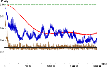
  Figure 1: Evolution of the purity for $\epsilon=0.1$ and $J_{0}=0$ (dashed green line), $J_{0}=0.3$ (red line), $J_{0}=1$ (blue line) and $J_{0}=1.5$ (brown line).We also depict the reference (black line) of the level of purity of a distribution of $N=5$ random projectors on $\mathbb{C}^{10}$.

• Instead, we can consider a fixed value of the initial classical momentum and increase the value of the coupling. It can be remarked that the system reaches the level of purity of the set of random projectors much faster than in the previous case, (see fig. 2).

  

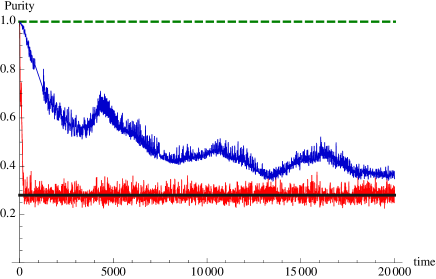
  Figure 2: Evolution of the purity for $J_{0}=0.8$ and $\epsilon=0$ (dashed green line), $\epsilon=0.1$ (blue line), and $\epsilon=0.2$ (red line). Again, the reference (black line) represents the level of purity of a distribution of $N=5$ random projectors on $\mathbb{C}^{10}$.

The interesting behaviour of the purity shown for some values of the parameters in figs. 1 (brown line) and 2 (red line), in which its value rapidly decreases to a given low one and fluctuates around it after that, can be explained as a consequence of the dynamics mentioned before. If the system exhibits sensitive dependence on the initial conditions, after a small lapse of time, the different trajectories become decorrelated from one another in the Hilbert space. Therefore, the density matrix becomes the normalized sum of $N$ rank one projectors chosen at random. In this situation, it can be shown (see appendix A) that the purity is distributed around an expected value

$$\operatorname{E}[\mathrm{Tr}(\rho^{2})]=\frac{N+D-1}{ND},$$ (55)

which is represented by the black straight lines in the figures, with fluctuations of size

$$\sigma:= \left(\operatorname{E}[\mathrm{Tr}(\rho^{2})^{2}]-\operatorname{E}[\mathrm{Tr}(\rho^{2})]^{2}\right)^{1/2}$$

$$= \frac{\sqrt{2}}{ND}\left(\frac{(N-1)(D-1)}{N(D+1)}\right)^{1/2},$$ (56)

where $N$ is the total number of trajectories used and $D$ is the dimension of the quantum Hilbert space. Notice that if $D$ is very large, the expected value for the purity tends to its minimal value $1/N$ and the fluctuations tend to zero. Remember that the degree of mixture of a quantum system ranges from the pure state case (i.e., purity equals to one), for which the density operator is a projector on a one dimensional subspace of the Hilbert space and the maximal mixture case (thus minimum purity) which corresponds to a density operator which is proportional to the identity matrix. As it must have trace equal to one, the proportionality factor is equal to the inverse of the dimension of the Hilbert space.

Figs. 1 and 2 show also the effect of the coupling between the classical and the quantum subsystems, as well as the effect of the momentum (or equivalently, the energy) of the classical particles on the evolution of purity. The greater the strength of the coupling and the energy of the classical particle, the faster the system reaches its asymptotic behavior. Although clearly the coupling has a stronger effect. Thus, analogously to what happens in the case of molecular dynamics, where the velocity of the classical nuclei induces the coupling between all the eigenstates of the electronic Hamiltonian, we see here that it also has the effect of mixing the quantum part if the Ehrenfest system is treated statistically.

From our analysis and example, we can then conclude that statistical Ehrenfest dynamics provides a framework in which the evolution affects the quantum dynamics in at least one way decoherence does. Changing the degree of mixture of the quantum state is certainly one of the most relevant effects of electronic decoherence on molecular systems, although further work is required to analyze whether or not other decoherence effects can be explained by our construction.

VI Conclusions and future work

An appropriate description of the electronic decoherence in molecular systems is on the wishlist of every quantum-classical dynamics scheme. In which amount each theoretical model includes the sought effects is a complicated question whose answer will depend both on the model and on the intended application. Loosely speaking, we could expect the different models to range from ‘no electronic decoherence at all’ (e.g., BOMD) to ‘a perfect description of quantum electronic decoherence’ (say, full quantum dynamics of electrons and nuclei), with most of them lying somewhere in between the two extremes. Several methods Truhlar (2007); Zhu, Jasper, and Truhlar (2005); Prezhdo (1999); Subotnik (2010); Horsfield et al. (2006); Tully (1990a, b, 1998); Landry and Subotnik (2011); Bedard–Hearn, Larsen, and Schwartz (2005); Sun, Wang, and Miller (1998); Subotnik and Shenvi (2011) have been developed to deal with the problem but, to our knowledge, without a definitive solution.

Pure Ehrenfest dynamics (ED for single states) clearly lies in the ‘no decoherence at all’ side of the spectrum, since it does not even allow the change of purity. However, if we are willing to accept the possibility that the electrons evolve into a mixed state, i.e., a statistically uncertain electronic state, then, to perform a coherent analysis, we should also allow the initial conditions of the nuclei to be described statistically. This point of view was used in some of the papers mentioned above when considered within surface-hopping or decay-of-mixing formalisms. In this work we implement the idea using the statistical description of Ehrenfest dynamics introduced in Ref. Alonso et al., 2011 combined with a specially convenient geometric formalism we introduce. Using these methods, one can observe that a system starting from uncertain nuclear initial conditions and a pure electronic state evolves into a situation in which the electronic state is no longer pure but mixed, i.e., ED is capable of transferring uncertainty between the nuclei and the electrons. Besides, our method provides us also with tools to compute in a simple but rigorous way the purity change, and it indicates an interesting dependence of the effect on the number of trajectories $N$ and the dimension of the Hilbert space $D$, as well as on the coupling and the velocity (or energy) of the classical system. ‘How much’ decoherence the statistical ED contains, as related to interesting practical applications or to other mixed quantum-classical schemes,Bittner and Rossky (1997, 1995) is a complex and important question that we shall explore in future works.

Appendix A Purity of a sum of random projectors of rank one

In this appendix we derive the expected value of the purity and its fluctuations when the density matrix is obtained from the sum of decorrelated, random, rank-one projectors.

The purity for a density matrix of the form

$$\rho=\frac{1}{N}\sum_{j=1}^{N}\frac{|\psi_{j}\rangle\langle\psi_{j}|}{\langle\psi_{j}|\psi_{j}\rangle}$$

is

$${\rm Tr}(\rho^{2})=\frac{1}{N^{2}}\left(N+2\sum_{j<k}\chi_{jk}\right),$$

where we have defined

$$\chi_{jk}:=\frac{|\langle\psi_{j}|\psi_{k}\rangle|^{2}}{\langle\psi_{j}|\psi_{j}\rangle\langle\psi_{k}|\psi_{k}\rangle}.$$

Next, we will determine the probability density for $\chi_{12}$ when $\psi_{1}$ and $\psi_{2}$ are two decorrelated random vectors.

Given the global $U(N)$ symmetry of the problem we can take the first vector to be

$$\psi_{1}=(a,0,\cdots,0),\quad a\in\mathbb{R},$$

and the second chosen at random. If we denote

$$\psi_{2}=(q_{1}+ip_{1},q_{2}+ip_{2},\dots,q_{N}+ip_{N}),$$

we get

$$\chi:=\chi_{12}=\frac{(q_{1}^{2}+p_{1}^{2})}{r^{2}},$$

where $r^{2}:=\sum_{j}(q_{j}^{2}+p_{j}^{2})$.

We also need the adequate probability measure in $M_{Q}$ that distributes the random vector $\psi_{2}$. It can be defined by

$$d\pi_{Q}=f(r^{2})d\mu_{Q},$$

where $f$ is a positive function chosen so that

$$\int_{M_{Q}}d\pi_{Q}=1.$$

As we shall see, the actual form of $f$ is not relevant for the distribution of the purity.

It will be convenient to write the probability measure in $M_{Q}=\mathbb{R}^{2}\times\mathbb{R}^{2D-2}$ in the following way:

$$d\pi_{Q}=f(z^{2}+R^{2})zdzd\theta R^{2D-3}dRd\Omega_{2D-3},$$

where $(z,\theta)$ represents polar coordinates in the plane $(q_{1},p_{1})$, $R$ is the radial coordinate in $\mathbb{R}^{2D-2}$ (i.e., $R^{2}:=\sum_{j>1}(q_{j}^{2}+p_{j}^{2})$), while the volume element $d\Omega_{2D-3}$ stands for the angular coordinates in $\mathbb{R}^{2D-2}$. In these coordinates $r=\sqrt{z^{2}+R^{2}}$ and $\chi=z^{2}/r^{2}$.

The next step is to perform the change of variables from $(R,z)$ to $(r,\chi)$. Taking into account that the Jacobian is

$$J=\frac{r}{2\sqrt{\chi(1-\chi)}},$$

one obtains

$$d\pi_{Q}=\frac{1}{2}f(r^{2})(1-\chi)^{D-2}d\chi r^{2D-1}drd\theta d\Omega_{2D-3},$$

and marginalizing out all variables except $\chi$ we find the needed measure:

$$d\pi_{\chi}=(D-1)(1-\chi)^{D-2}d\chi.$$

Once we have determined the probability distribution for $\chi$ we can compute the average value for the purity. Using the expression at the beginning of this appendix,

$$\operatorname{E}[\mathrm{Tr}(\rho^{2})]=\frac{1}{N^{2}}\left(N+2\sum_{j<k}\operatorname{E}[\chi_{ij}]\right)=\frac{1}{N}\Big{(}1+(N-1)\operatorname{E}[\chi]\Big{)},$$ (57)

where we have used that all random variables $\chi_{ij}$ are identically distributed.

Finally, given that

$$\operatorname{E}[\chi]=\int_{0}^{1}\chi d\pi_{\chi}=\frac{1}{D},$$

we obtain the sought result:

$$\operatorname{E}[\mathrm{Tr}(\rho^{2})]=\frac{N+D-1}{ND}.$$

As for the fluctuation, one has

$$\sigma^{2} =\frac{4}{N^{4}}\sum_{j<k}(\operatorname{E}[\chi_{jk}^{2}]-\operatorname{E}[\chi_{jk}]^{2})$$

$$=\frac{2(N-1)}{N^{3}}(\operatorname{E}[\chi^{2}]-\operatorname{E}[\chi]^{2})=\frac{2(N-1)}{N^{3}}\frac{(D-1)}{D^{2}(D+1)},$$ (58)

where we have used that

$$\operatorname{E}[\chi^{2}]=\frac{2}{D(D+1)}.$$

Appendix B Derivatives of the purity

In sec. IV.2, we explained how an initial uncertainty in the classical part of the state of an Ehrenfest system produces a change in the purity at $t=0$, even if the initial state is quantum-pure. In this appendix, we present in more detail the calculations that led us to that conclusion.

First of all, we need the first time-derivative of the purity. We know that the evolution of the $\rho(t)$ is given by Eq. (33). Then, the evolution of the purity can be written as:

$$\frac{d}{dt}\langle\rho(t)\rangle= 2\mathrm{Tr}\big{(}\dot{\rho}(t)\rho(t)\big{)}$$

$$= \int d\mu d\mu^{\prime}FF^{\prime}\mathrm{Tr}\big{(}i\hbar^{-1}[P_{\psi},H_{e}]\cdot P_{\psi^{\prime}}\big{)}$$

$$= i\hbar^{-1}\int d\mu d\mu^{\prime}FF^{\prime}\mathrm{Tr}\big{(}[P_{\psi},P_{\psi^{\prime}}]\cdot H_{e}\big{)},$$ (59)

where the integral is taken over $(M_{Q}\times M_{C})^{2}$, and we have denoted

$$d\mu :=d\mu_{QC}(\xi,\psi),$$ (60a)

$$d\mu^{\prime} :=d\mu_{QC}(\xi^{\prime},\psi^{\prime}),$$ (60b)

$$F :=F_{QC}(\xi,\psi),$$ (60c)

$$F^{\prime} :=F_{QC}(\xi^{\prime},\psi^{\prime}),$$ (60d)

$$H_{e} :=H_{e}(\xi),$$ (60e)

$$H^{\prime}_{e} :=H_{e}(\xi^{\prime}),$$ (60f)

$$P_{\psi} :=\frac{|\psi\rangle\langle\psi|}{\langle\psi|\psi\rangle},$$ (60g)

$$P_{\psi^{\prime}} :=\frac{|\psi^{\prime}\rangle\langle\psi^{\prime}|}{\langle\psi^{\prime}|\psi^{\prime}\rangle}.$$ (60h)

In the last step, we also used that

$$\mathrm{Tr}\big{(}[P_{\psi},H_{e}]\cdot P_{\psi^{\prime}}\big{)} =\mathrm{Tr}\big{(}P_{\psi}\cdot H_{e}\cdot P_{\psi^{\prime}}-H_{e}\cdot P_{\psi}\cdot P_{\psi^{\prime}}\big{)}$$

$$=\mathrm{Tr}\big{(}H_{e}\cdot P_{\psi^{\prime}}\cdot P_{\psi}-H_{e}\cdot P_{\psi}\cdot P_{\psi^{\prime}}\big{)}$$

$$=\mathrm{Tr}\big{(}H_{e}\cdot[P_{\psi},P_{\psi^{\prime}}]\big{)}$$

$$=\mathrm{Tr}\big{(}[P_{\psi},P_{\psi^{\prime}}]\cdot H_{e}\big{)}.$$

Also, as it is common in statistical dynamics, we can assign the time-evolution of the state to the probability distribution $F_{QC}$ and see the objects $\xi$, $\xi^{\prime}$ and $|\psi\rangle$, $|\psi^{\prime}\rangle$ just as the initial conditions, or we can alternatively think that $F_{QC}$ is the static distribution of initial conditions and consider that the time-evolving objects are $\xi$, $\xi^{\prime}$ and $|\psi\rangle$, $|\psi^{\prime}\rangle$. Either dynamical image is valid, and the two of them produce, of course, the same result, but we have performed the calculation thinking in the second way, which looked to us slightly more direct.

Now, in our example, $P_{\psi}(t=0)=P_{\psi^{\prime}}(t=0)=P_{\psi_{0}}$. Then, we see that the commutator $[P_{\psi},P_{\psi^{\prime}}]$ vanishes. Thus, we can conclude that:

$$\frac{d}{dt}\langle\rho(t)\rangle\Big{|}_{t=0}=0.$$ (61)

Using again Eq. (5)-(7), we can also compute the second derivative of the density matrix,

$$\ddot{\rho}(t)=\int d\mu F \left(i\hbar^{-1}\big{(}\big{[}\{H_{e},f_{H}\}_{C},P_{\psi}\big{]}\big{)}\right.$$

$$-\hbar^{-2}\left.\big{(}\big{[}H_{e},\big{[}H_{e},P_{\psi}]\big{]}\big{)}\right),$$ (62)

where we have used the same notation in eqs. (60), and the integral is this time extended to $M_{Q}\times M_{C}$. With this expression, we can compute the second derivative of the purity:

$$\frac{d^{2}}{dt^{2}}\langle\rho(t)\rangle=\mathrm{Tr}\Big{(}\rho(t)\ddot{\rho}(t)+(\dot{\rho}(t))^{2}\Big{)}.$$ (63)

Now, using eqs. (33), (B) and (B) we can calculate a more explicit form for this second derivatives in terms of the objects associated to the geometric formalism

$$\frac{d^{2}}{dt^{2}}\langle\rho(t)\rangle=\int d\mu d\mu^{\prime}FF^{\prime}\left[i\hbar^{-1}\mathrm{Tr}\Big{(}\big{[}\{H_{e},f_{H}\},P_{\psi}\big{]}\cdot P_{\psi^{\prime}}\Big{)}\right.$$

$$- \hbar^{-2}\mathrm{Tr}\Big{(}\big{[}H_{e},[H_{e},P_{\psi}]\big{]}\cdot P_{\psi^{\prime}}\Big{)}$$

$$- \left.\hbar^{-2}\mathrm{Tr}\Big{(}\big{[}H_{e},P_{\psi}\big{]}\cdot\big{[}H^{\prime}_{e},P_{\psi^{\prime}}\big{]}\Big{)}\right]$$

$$=\int d\mu d\mu^{\prime}FF^{\prime}\left[i\hbar^{-1}\mathrm{Tr}\Big{(}\big{[}\{H_{e},f_{H}\},P_{\psi}\big{]}\cdot P_{\psi^{\prime}}\Big{)}\right.$$

$$+ \hbar^{-2}\mathrm{Tr}\Big{(}\big{[}H_{e},P_{\psi}\big{]}\cdot\big{[}H_{e},P_{\psi^{\prime}}\big{]}\Big{)}$$

$$- \left.\hbar^{-2}\mathrm{Tr}\Big{(}\big{[}H_{e},P_{\psi}\big{]}\cdot\big{[}H^{\prime}_{e},P_{\psi^{\prime}}\big{]}\Big{)}\right]$$

$$=\int d\mu d\mu^{\prime}FF^{\prime}\left[i\hbar^{-1}\mathrm{Tr}\Big{(}\big{[}\{H_{e},f_{H}\},P_{\psi}\big{]}\cdot P_{\psi^{\prime}}\Big{)}\right.$$

$$+ \left.\hbar^{-2}\mathrm{Tr}\Big{(}\big{[}H_{e},P_{\psi}\big{]}\cdot\big{[}(H_{e}-H^{\prime}_{e}),P_{\psi^{\prime}}\big{]}\Big{)}\right],$$

where we used that

$$\mathrm{Tr}\Big{(}\big{[}H_{e},[H_{e},P_{\psi}]\big{]}\cdot P_{\psi^{\prime}}\Big{)}=\mathrm{Tr}\Big{(}\big{[}H_{e},P_{\psi}\big{]}\cdot\big{[}H_{e},P_{\psi^{\prime}}\big{]}\Big{)}.$$

Using this expression, it is finally straightforward to compute the second derivative at $t=0$ for the distribution $F_{QC}$ given by Eq. (44):

$$\frac{d^{2}}{dt^{2}}\langle\rho(t)\rangle\Big{|}_{t=0}= -\frac{\hbar^{-2}}{2}\mathrm{Tr}\left(\big{[}H_{e}(\xi_{0}^{1})-H_{e}(\xi_{0}^{2}),P_{\psi_{0}}\big{]}^{2}\right)$$

$$= -\hbar^{-2}\langle\psi_{0}|\big{(}H_{e}(\xi_{0}^{1})-H_{e}(\xi_{0}^{2})\big{)}^{2}|\psi_{0}\rangle$$

$$+\hbar^{-2}\langle\psi_{0}|\big{(}H_{e}(\xi_{0}^{1})-H_{e}(\xi_{0}^{2})\big{)}|\psi_{0}\rangle^{2}.$$ (65)

References

- Alonso et al. (2011) J. L. Alonso, A. Castro, J. Clemente-Gallardo, J. C. Cuchí, P. Echenique, and F. Falceto, J. Phys. A: Math. Theor. 44, 396004 (2011).
- Andrade et al. (2009) X. Andrade, A. Castro, D. Zueco, J. L. Alonso, P. Echenique, F. Falceto, and A. Rubio, J. Chem. Theor. Comp. 5, 728 (2009).
- Tully (1990a) J. C. Tully, J. Chem. Phys. 93, 1061 (1990a).
- Zhu, Jasper, and Truhlar (2005) C. Zhu, A. W. Jasper, and D. G. Truhlar, J. Chem. Theor. Comp. 1, 527 (2005).
- Truhlar (2007) D. G. Truhlar, “Decoherence in combined quantum mechanical and classical mechanical methods for dynamics as illustrated for non–Born–Oppenheimer trajectories,” in Quantum Dynamics of Complex Molecular Systems, edited by D. A. Micha and I. Burghardt (Springer, Berlin, 2007) pp. 227–243.
- Prezhdo (1999) O. V. Prezhdo, J. Chem. Phys. 111, 8366 (1999).
- Subotnik (2010) J. E. Subotnik, J. Chem. Phys. 132, 134112 (2010).
- Horsfield et al. (2006) A. P. Horsfield, D. R. Bowler, H. Ness, C. G. Sánchez, T. N. Todorov, and A. J. Fisher, Rep. prog. Phys. 69, 1195 (2006).
- Tully (1990b) J. C. Tully, “Nonadiabatic dynamics,” in Modern Methods for Multidimensional Dynamics Computations in Chemistry, edited by D. Thompson (World Scientific, Singapore, 1990) p. 34.
- Tully (1998) J. C. Tully, “Mixed quantum-classical dynamics: Mean-field and surface-hopping,” in Classical and Quantum Dynamics in Condensed Phase Simulation, edited by B. G. Berne, G. Ciccotti, and D. F. Coker (World Scientific, Singapore, 1998) pp. 489–515.
- Landry and Subotnik (2011) B. R. Landry and J. E. Subotnik, J. Chem. Phys. 135, 191191 (2011).
- Bedard–Hearn, Larsen, and Schwartz (2005) M. J. Bedard–Hearn, R. E. Larsen, and B. J. Schwartz, J. Chem. Phys. 123, 234106 (2005).
- Sun, Wang, and Miller (1998) X. Sun, H. Wang, and W. H. Miller, J. Chem. Phys. 109, 7064 (1998).
- Subotnik and Shenvi (2011) J. E. Subotnik and N. Shenvi, J. Chem. Phys. 134, 244114 (2011).
- Schlosshauer (2007) M. Schlosshauer, Decoherence and the Quantum-to-Classical Transition (Springer, 2007).
- Zurek (2003) W. H. Zurek, Rev. Mod. Phys. 75, 716 (2003).
- Mauri, Car, and Tossati (1993) F. Mauri, R. Car, and E. Tossati, Europhys. Lett. 24, 431 (1993).
- Parandekar and Tully (2006) P. V. Parandekar and J. C. Tully, J. Chem. Theor. Comp. 2, 229 (2006).
- Parandekar and Tully (2005) P. V. Parandekar and J. C. Tully, J. Chem. Phys. 122, 094102 (2005).
- Schmidt, Parandekar, and Tully (2008) J. R. Schmidt, P. V. Parandekar, and J. C. Tully, J. Chem. Phys. 129, 044104 (2008).
- Bastida et al. (2007) A. Bastida, C. Cruz, J. Zúñiga, A. Requena, and B. Miguel, J. Chem. Phys. 126, 014503 (2007).
- Alonso et al. (2010) J. L. Alonso, A. Castro, P. Echenique, V. Polo, V. Rubio, and D. Zueco, N. J. Phys. 12, 083064 (2010).
- Alonso et al. (2012) J. Alonso, A. Castro, P. Echenique, and A. Rubio, in Fundamentals of Time-Dependent Density Functional Theory, edited by M. Margues et al. (Lecture Notes in Physics 837, Springer, 2012).
- Marx and Hutter (2000) D. Marx and J. Hutter, “Modern methods and algorithms of quantum chemistry,” (Jülich. John von Neumann Institute for Computing, 2000) Chap. Ab initio molecular dynamics: Theory and implementation, pp. 329–477.
- Teilhaber (1992) J. Teilhaber, Phys. Rev. B 46, 12990 (1992).
- Kalia et al. (1990) R. K. Kalia, P. Vashishta, L. H. Yang, F. W. Dech, and J. Rowlan, Intl. J. Supercomp. Appl. 4, 22 (1990).
- Meyer and Miller (1979) H. Meyer and W. H. Miller, J. Chem Phys. 70, 3214 (1979).
- Kibble (1979) T. W. B. Kibble, Com. Math. Phys. 65, 189 (1979).
- Heslot (1985) A. Heslot, Phys. Rev. D 31, 1341 (1985).
- Brody and Hughston (2001) D. C. Brody and L. P. Hughston, J. of Geom. and Phys. 38, 19 (2001).
- Cariñena, Clemente-Gallardo, and Marmo. (2007) J. F. Cariñena, J. Clemente-Gallardo, and G. Marmo., Theor. Math. Phys. 152, 894 (2007).
- Cohen–Tannoudji, Laloë, and B. Diu (1977) C. Cohen–Tannoudji, F. Laloë, and B. B. Diu, Quantum Mechanics (Hermann, Paris, 1977).
- Gleason (1957) A. M. Gleason, J. of Mathematics and Mechanics 6, 885 (1957).
- Breuer and Petruccione (2002) H. P. Breuer and F. Petruccione, The theory of open quantum systems (Oxford University Press, 2002).
- Note (2) The Mathematica notebook containing all the programs used in this section can be found as supplementary material.
- Bittner and Rossky (1997) E. R. Bittner and P. J. Rossky, J. Chem. Phys 107 (1997).
- Bittner and Rossky (1995) E. R. Bittner and P. J. Rossky, The Journal of Chemical Physics 103, 8130 (1995).