Measurement of the gradient of the Casimir force between a nonmagnetic sphere and a magnetic plate

Abstract

We measured the gradient of the Casimir force between an Au sphere and a plate made of ferromagnetic metal (Ni). It is demonstrated that the magnetic properties influence the force magnitude. This opens prospective opportunities for the control of the Casimir force in nanotechnology and for obtaining Casimir repulsion by using ferromagnetic dielectrics.

I Introduction

In the last few years the Casimir effect 1 has attracted much experimental and theoretical attention as a fluctuation-induced quantum phenomenon with diverse applications ranging from nanotechnology to elementary particle physics, gravitation and cosmology.2 ; 3 Many experiments on measuring the Casimir force in configurations with material boundaries made of nonmagnetic metals, semiconductors and dielectrics have been performed (see reviews 4 ; 5 ; 6 ). On the theoretical side, the Lifshitz theory 7 of the van der Waals and Casimir forces between plane-parallel plates described by the frequency-dependent dielectric permittivity $\varepsilon(\omega)$ was generalized for the boundary surfaces of arbitrary shape 8 ; 9 ; 10 . Nevertheless, application of this theory to materials with free charge carriers is under much discussion.3 ; 4 ; 6 ; 22 ; 23 ; 24 ; 25 ; 10a ; 10b ; 10L ; 10c ; 10d ; 10e ; 11 ; 12 ; 12a ; 12b

The Lifshitz theory has long been generalized 13 for the case of magnetic materials described by the frequency-dependent magnetic permeability $\mu(\omega)$. The Casimir force between magnetodielectric plates was studied theoretically by many authors (see, e.g., 14 ; 15 ; 16 ; 17 ; 18 ; Rosa ; 19 ; 19a ), especially in connection with the possibility of Casimir repulsion, which has promise for nanotechnology. A large contribution of magnetic properties to the Casimir force (including the Casimir repulsion through a vacuum gap) was predicted 18 for constant $\varepsilon$ and $\mu$. For real magnetic metals described by the Drude model at nonzero temperature the effect of repulsion was not confirmed.15 ; 19 In Refs. 15 ; 20 it was shown that for real magnetic materials at room temperature the influence of magnetic properties on the Casimir force can occur solely through the zero-frequency contribution to the Lifshitz formula (the reason is that $\mu(i\xi)$ drops to unity at $\xi$ several orders of magnitude lower than the first Matsubara frequency). It was also predicted Rosa ; 20 that in the interaction of a nonmagnetic metal with a ferromagnetic dielectric the Casimir repulsion is possible if the relaxation properties of free electrons in a metal and the dc conductivity of the dielectric are omitted. Keeping in mind that some measurements 10a ; 10b ; 10L ; 10e ; 11 ; 12 ; 12a ; 12b have raised questions on whether the relaxation properties of free charge carriers and dc conductivity influence the Casimir force, there is a question pointed out in Ref. 20 if the magnetic properties of real materials will influence the Casimir force.

This paper starts the experimental investigation of the Casimir effect in the presence of magnetic boundaries. Using the dynamic atomic force microscope (AFM), operated in a frequency shift technique, we have measured the gradient of the Casimir force between an Au-coated sphere and a plate covered with the ferromagnetic metal Ni. The experimental data were compared with predictions of the Lifshitz theory extrapolated to zero frequency both including 22 ; 23 and omitting 24 ; 25 the relaxation properties of free electrons (i.e., using the Drude and plasma model approaches discussed in the literature.3 ; 4 ) It was found that the measurement data are in excellent agreement with the predictions of the plasma model approach taking the magnetic properties into account and with the Drude model approach (which is not sensitive to magnetic properties for a nonmagnetic metal interacting with the magnetic one). Predictions of both these approaches are shown to be very close within the range of experimental separations $220\,\mbox{nm}\leq a\leq 500\,$nm. If to combine the obtained results with an exclusion of the Drude model approach for nonmagnetic metals found in several experiments 10a ; 10b , one can consider our experiment as a confirmation of the influence of magnetic properties on the Casimir force. This opens outstanding opportunities for the tuning of the Casimir force in nanotechnology by means of depositing ferromagnetic films on movable parts of microdevices and even obtaining repulsive Casimir forces (other means are considered in Refs.4 ; 5 ; 28 ; P ).

The paper is organized as follows. In Sec. II we describe the measurement scheme and the experimental setup using a dynamic AFM. Section III is devoted to the calibration procedures and measurement results. Section IV contains comparison between experiment and theory. In Sec. V the reader will find our conclusions and discussion.

II Measurement scheme and experimental setup

We have applied different voltages $V_{i}$ to the plate and measured the gradient of the total force, electric plus Casimir,

$$F_{\rm tot}(a)=F_{\rm el}(a)+F(a),$$ (1)

between an Au-coated sphere of radius $R$ and Ni-coated plate using dynamic force microscopy, more specifically, frequency modulation AFM.26 It was originally conceived as a technique to explore short-range forces. The sensing element of this technique is the change of resonant frequency of a periodically driven cantilever, where the change is proportional to the gradient of the force. It is always assumed that the amplitude of the oscillation of the cantilever is small. In this technique the driving frequency is kept near the resonance frequency of the cantilever to obtain the highest signal to noise. Note that previous experiments on measuring the Casimir force by means of dynamic AFM used the phase shift 27 and the amplitude shift 28 techniques. These have not been as precise as the frequency modulation technique. For small oscillations of the cantilever, the change in the frequency $\Delta\omega=\omega_{r}-\omega_{0}$, where $\omega_{r}$ is the resonance frequency in the presence of external force $F_{\rm tot}$ and $\omega_{0}$ is the natural resonance frequency, is given by

$$\Delta\omega=-\frac{\omega_{0}}{2k}\left(\frac{\partial F_{\rm el}}{\partial a}+\frac{\partial F}{\partial a}\right)=-\beta(V_{i}-V_{0})^{2}-C\frac{\partial F}{\partial a}.$$ (2)

Here, $C\equiv C(k,\omega_{0})=\omega_{0}/(2k)$, $\beta\equiv\beta(a,z_{0},C,R)=C\partial X(a,R)/\partial a$, $k$ is the spring constant of the cantilever, absolute separations $a=z_{\rm piezo}+z_{0}$, where $z_{\rm piezo}$ is the plate movement due to the piezoelectric actuator and $z_{0}$ is the point of the closest approach between the Au sphere and Ni plate, and $X(a,R)$ is a known function.3 ; 4 ; 10a ; 12 The residual potential difference $V_{0}$ in (2) can be nonzero even for a grounded sphere due to the different work functions of the sphere and plate materials or contaminants on the interacting surfaces.

Expression (2) is the basis of the technique used in this experimental study to explore the Casimir effect in magnetic materials. The electrostatic force gradient and therefore the frequency shift has a parabolic dependence on the voltage $V_{i}$ applied to the plate. From Eq.(2), the minimum in the frequency shift corresponds to $V_{0}$. The curvature of the parabola, which includes the spatial dependence of the electrostatic force and the cantilever parameters, is related to $\beta$ and depends on $z_{0}$ and $C$. Thus these parameters can be extracted from this dependence. In order to test for systematic errors in the fitting parameters, the fitting is repeated at many different distance ranges.

The instrument was designed for a precision measurement of the Casimir force gradient. The primary pieces of equipment necessary for frequency modulation measurements consist of a microfabricated cantilever, the cantilever motion controllers (piezoelectric transducers), plate motion controller (piezoelectric tube), optical detection system, and a phase locked loop (PLL) to measure the frequency shift. The cantilever was placed inside a high vacuum chamber. All these allowed us to reach subnanometer separation distance resolution over a distance range larger than two micrometers.

The sphere was attached to the cantilever. The chosen sphere needs to have a large $R$ and a smooth clean surface. To attach it to the cantilever we used a dot of Ag epoxy at the tip of the free-end of the rectangular cantilever. To achieve high resonance frequencies and high signal to noise, hollow glass microspheres (3M Scotchlite) and stiff rectangular conductive Si cantilevers were used. The amount of epoxy has to be minimal to obtain the high frequencies. We used commercial monocrystalline cantilevers that are n-type and have a specific resistance of 0.01 to 0.05 $\Omega\,$cm. We chosen them because they have very low amount of internal stresses, in comparison to other materials like silicon nitride (SiN₃). This leads to low energy dissipation, resulting in a high quality factor $Q$. We chosen ones with the smallest spring constant ($\sim 0.03\,$N/m). The cantilevers were cleaned with high-purity acetone and then rinsed with distilled and deionized water. After that, the silicon dioxide (SiO₂) layer on the surface of the cantilever was etched with a solution of HF for 1 min. Finally, they were double rinsed in a solution of deionized water. The Si cantilevers are conductive, which is necessary for good electrical contact to the sphere.

The surfaces of the hollow glass spheres are smooth as they are made from liquid phase. We used the special procedure for cleaning the spheres before attachment to the cantilever to remove organic contaminants and debris from the surface. Details of this procedure are described in Ref. 10b .

The next step was to thermally evaporate a uniform coating of $280\pm 1\,$nm of Au on the sphere and at the top of the free end of the cantilever. The Au on the top of the cantilever has to be evaporated only at the tip, about 50 $\mu$m from the free end. The radius of the sphere was measured to be $R=64.1\pm 0.1\,\mu$m using a SEM. The tip of the cantilever and sphere were coated with Au using a specially designed mask. Coating only the cantilever tip, preserves the large oscillation $Q$-factor leading to high sensitivity. We used an oil-free thermal evaporator for the Au coating. This instrument is equipped with a scroll pump (“Varian”, SH-100) and a turbomolecular pump (“Varian”, TV301 Navigator) that permits us to coat at a pressure of $10^{-6}\,$Torr. To achieve uniformity the cantilever sphere system was rotated using a motor during evaporation. To obtain a smooth coating, the coating rate has to be low and done with cooler atoms. The Au coating was done over 4 hours, at a boat-cantilever distance of about $2.5^{\prime\prime}$ to achieve a uniform 280 nm thick layer. To obtain smooth coatings, it was found that an equilibrium pressure be reached after melting of the Au wire, before start of the coating process.

We used a Si plate as substrate for the Ni coating. The plate was first cleaned in acetone for 15 min using a sonicator, then rinsed with deionized water. This was repeated in IPA for another 15 min and rinsed with deionized water. Finally it was cleaned in ethanol for 15 min again using a sonicator and blow dried in nitrogen. To increase adhesion we placed the substrate in a UV chamber for 30 min. Next we inserted the substrate in a E-beam evaporator (“Temescal systems”, model BJD-1800) for Ni coating. A vacuum of $10^{-6}\,$Torr was used. The rotation of the sample was done to provide the uniform Ni coating. To obtain a coating rate of $\sim 3\,$Å/s, the high voltage supply controlling the electron beam was kept at 10.5 kV and filament current at 0.5 A. The thickness of the Ni coating was measured with an AFM to be $154\pm 1\,$nm. The roughness of the Au and Ni coatings was measured using an AFM at the end of the experiment.

The cantilever with the Au-coated sphere was clamped in a specially fabricated holder containing two piezos. The first piezo was connected to a closed proportional-integral-derivative (PID) controller. The second was connected to the PLL. The Ni plate was mounted on top of a $3^{\prime\prime}$ segmented piezoelectric tube capable of traveling a distance of $2.3\,\mu$m. Using a $3^{\prime\prime}$ segmented piezoelectric tube allows us to achieve large separation between the substrate with subnanometer spatial resolution. Ohmic contacts were made to the Ni plate through a 1 k$\Omega$ resistor. The calibration of the plate piezo was done using the fiber interferometer and is described in previous work.29 A continuous 0.01 Hz triangular voltage signal was applied to the piezoelectric actuator to change the sphere-plate distance and avoid piezo drift and creep. The experiments were performed in a vacuum of $3\times 10^{-8}\,$Torr at room temperature.

The main vacuum chamber was a $8^{\prime\prime}$ six-way stainless steel cross. The chamber was evacuated by a turbo-pump (“Varian Inc.”, V-301) followed by an oil-free dry scroll pump (“Leybold Vac.”, SC-15D). The main vacuum chamber was mounted on a $8^{\prime\prime}$ ion pump (“Varian Inc.” Diode). The chamber was separated from the turbo pump by gate valve ($6^{\prime\prime}$ viton o-ring sealed gate with stainless steel construction) which can be closed to isolate the turbo pump from the chamber. During data acquisition only the ion pump was used and the turbo pump was valved off and shut off to reduce the mechanical noise. The chamber was supported on a damped optical table having a large mass to reduce the mechanical noise.

We detected the cantilever oscillations and Ni plate displacements with two fiber interferometers. The first interferometer monitored the cantilever oscillation. The second recorded the displacement of the Ni plate mounted on the AFM piezoelectric transducer. These custom-built interferometers consist of a laser diode pigtail, various types of fiber couplers and photodiodes for detecting the interferometric signal. Since all junctions between the components of the interferometer were spliced, stray interference and retroreflection to the laser diodes were minimized. In addition, to minimize laser and wavelength fluctuations, the temperature and power of the laser diodes were kept constant using feedback circuits.

Below we describe the first interferometer, which was used for monitoring the resonant frequency of the cantilever. The interferometric cavity was formed with the cleaved end of an optical fiber and the top free end of the microcantilever. The cantilever chip holder sits on top of two small piezoelectrics, one for oscillating the cantilever and the second for changing the length of the interferometric cavity. For constructing the interferometer, we used a 1550 nm (“Thorlabs Inc.”, 1550B-HP) single mode fiber which has extremely low bending loss and low splice loss. A super luminescent diode (“Covega Co”, SLD-1108) with a wavelength of 1550 nm and a coherence length of 66 $\mu$m served as the light source for the cantilever frequency measurement interferometer. The short coherence length prevents spurious interferences. In addition, an optical isolator with FC-APC connectors connected the diode to a 50/50 directional coupler to reduce undesirable reflections. A typical fused-tapered bi-conic coupler at 1550 nm wavelength with return-loss of –55dB was used as input. To position the fiber end vertically above and close to the cantilever, an $xyz$-stage as described in Ref. 10b was used.

The second interferometer, which was used for detecting the distance moved by the Ni plate travel, had the same fabrication techniques. The only difference is the fiber coupled laser source (“Thorlabs Inc.”, S1FC635) with a wavelength of 635 nm.

Now we consider the interferometer system used for measuring the frequency shift. The output light was measured with InGaAs photodetectors. For the cantilever interferometer a low noise photodetector amplifier system was constructed using a balanced InGaAs photodiode coupled to an OPA627 low noise operational amplifier. The output of the interference signal was fed into a band-pass filter (“SRS Inc.”, SR650, with the range set between $1.20-1.85\,$kHz) cascaded by low (“SRS Inc.”, SR965, 260 Hz) and high (“SRS Inc.”, SR965, 1 kHz) pass filters to cut off unwanted frequency bands. The high-pass filter helped us to remove the noise in the excitation signal from frequency modulation controller and the low-pass filter cleaned the signal to the PID loop.

For frequency demodulation we used a PLL. The PLL frequency demodulator system combines a controller module to maintain the resonant frequency and a detector module to measure the force gradient induced resonant frequency shift. A piezoelectric actuator connected to the output of the PLL drives the cantilever at its resonant frequency with a constant amplitude. For all separations the oscillation amplitude of the cantilever was fixed at $<10\,$nm. To control the amplitude, the fluctuation spectrum of the cantilever was measured with a spectrum analyzer. The latter was calibrated using the thermal noise oscillation spectrum which has an average amplitude of $\sim 0.4\,$nm. During experiment the signal on the spectrum analyzer was about 15 times higher than for the thermal noise. The output of the low pass filter was used to form a closed loop PID controller using a piezoelectric actuator, to maintain constant separation distance between the fiber end and the cantilever. LabView software was used to control and monitor PID function and to acquire the data. The program also sets the voltages applied to the Ni plate using a low-noise voltage supply.

III Calibration procedures and measurement results

The frequency shift of our oscillator due to the total force (electrostatic and Casimir) between the Au sphere and the Ni plate was measured as a function of sphere-plate separation distance. For this purpose, the Ni-coated plate was connected to a voltage supply (33220A, “Agilent Inc.”) operating with $1\,\mu$V resolution. 11 different voltages in the range from –87.1 to 25.9 mV were applied to the Ni plate, while the sphere remained grounded. The plate was moved towards the sphere starting at the maximum separation, and the corresponding frequency shift was recorded at every 0.14 nm. This measurement was repeated four times. Any mechanical drift was subtracted from the separation distance. To do so we took into account that at $a>2\,\mu$m, the total force between the sphere and plate is below the instrumental sensitivity. At these separations, the noise is far greater than the signal and in the absence of systematic errors the signal should average to zero. However, the drift caused the separation distance to increase by around 1 nm in 1000 s, where 100 s correspond to time taken to make the one measurement (note that positional precision much better than 1 nm was achieved in this experiment). The drift rate was calculated from the change in position at one frequency shift signal plotted as a function of time. This procedure was repeated for 15 different frequency shift signals to calculate the average drift rate, which was found to be 0.002 nm/s. The separation distance in all measurements was corrected for this drift rate. Note that the temperature was controlled through excellent thermal contact to the heat bath, which is the large thermal mass of the vacuum chamber and optical table. The experiment was equilibriated for several hours before data were taken. The drift was experimentally found to be linear during 40 min, which is the time scale of the measurements (see Ref.10b for details where the same setup was used).

After applying the drift correction the residual potential $V_{0}$ between the sphere and plate was determined using the following procedure. For every 1 nm separation the frequency shift signals were found by interpolation. Then these signals were plotted as a function of the applied voltage $V_{i}$ at every separation and the corresponding $V_{0}$ identified at the position of the parabola maxima. The curvature of the parabola $\beta$ was also found. These $V_{0}$ from all four measurement sets are plotted in Fig. 1(a) versus separation distance. In Fig. 1(b) we show the systematic error of each individual $V_{0}$, as determined from the fit, at different separations. The mean value is $V_{0}=-34.1\pm 1\,$mV, where the total error is determined at a 67% confidence level, and can be observed to be independent of separation. This is an indirect confirmation of the fact that the interacting regions of the surfaces are clean or the adsorbed impurities are randomly distributed with a sub-micrometer length scales and do not contribute to the total force.10b

The next step was to determine the separation distance at closest approach $z_{0}$ and the coefficient $C$ in Eq. (2). As discussed above, these parameters associated with the cantilever can be found from the dependence of the parabola curvature $\beta$ on distance. The corresponding theoretical expression for parabola curvature was fit to $\beta$ as function of the separation distance. A least $\chi^{2}$ procedure was used in the fitting and the best values of $z_{0}$ and $C$ were obtained. The fitting procedure was repeated by keeping the start point fixed at the closest separation, while the end point measured from the closest separation was varied from 750 to 50 nm. The values of $z_{0}$ shown in Fig. 2(a) are seen to be independent of the end point position indicating the absence of systematic errors resulting from $z_{\rm piezo}$ calibration, mechanical drift etc. The systematic errors of each individual $z_{0}$, as determined from the fit, vary between 0.32 and 0.45 nm. Similarly, the values of the coefficient $C$ shown in Fig. 2(b) were also extracted by fitting the $\beta$-curve as a function of separation. The systematic errors of each individual $C$ vary between 0.13 and 0.18 kHz m/N. The independence of $C$ on separation again indicates the absence of systematic errors. The mean values obtained were $z_{0}=217.1\pm 0.4$ nm and $C=46.7\pm 0.15\,$kHz m/N, respectively (see Ref.10b for details). After the determination of $z_{0}$ the absolute sphere-plate separations can be found. Using $C$ and the measured frequency shifts, the gradients of the Casimir force were calculated from Eq. (2).

We now turn to the determination of the experimental errors. The random error in the gradient of the Casimir force calculated from 44 repetitions (4 measurement sets with 11 applied voltages each) at a 67% confidence level is shown by the short-dashed line in Fig. 3. The systematic error is determined by the instrumental noise including the background noise level, by the errors in calibration and by the error in the gradient of electrostatic force subtracted in accordance with Eq. (2) to get $F^{\prime}(a)$. It is shown by the long-dashed line in Fig. 3. The total experimental error found at a 67% confidence level is shown by the solid line in Fig. 3. The error in separation $\Delta a=0.4\,$nm coincides with the error in the determination of $z_{0}$ (details of error analysis can be found in Ref.10b ).

In Fig. 4(a-d) the measured gradients of the Casimir force are indicated as crosses, where the arms of the crosses are determined by the total experimental errors. It can be seen that the total relative experimental error in the measurements of $F^{\prime}(a)$ at $a=220$, 250, 300, 400, and 500 nm is equal to 0.6%, 0.94%, 1.8%, 5.4%, and 12.8%, respectively.

IV Comparison between experiment and theory

Now we compare the experimental data for the gradient of the Casimir force in the configuration containing nonmagnetic (Au) and magnetic (Ni) metals with the predictions of the Lifshitz theory. Computations were performed using the following Lifshitz-type formula 20 for $F^{\prime}(a)$ obtained in the sphere-plate geometry with the help of the proximity force approximation (using the exact theory, it was recently shown 30 ; 31 that the error in this case is less than $a/R$, i.e., less than 0.3% at the shortest separation):

$$F^{\prime}(a,T)=2k_{B}TR\sum_{l=0}^{\infty}{\vphantom{\sum}}^{\prime}\int_{0}^{\infty}q_{l}k_{\bot}dk_{\bot}$$ (3)

$$~{}\times\left[\frac{r_{\rm TM}^{\rm(Au)}r_{\rm TM}^{\rm(Ni)}}{e^{2aq_{l}}-r_{\rm TM}^{\rm(Au)}r_{\rm TM}^{\rm(Ni)}}+\frac{r_{\rm TE}^{\rm(Au)}r_{\rm TE}^{\rm(Ni)}}{e^{2aq_{l}}-r_{\rm TE}^{\rm(Au)}r_{\rm TE}^{\rm(Ni)}}\right].$$

Here, $k_{B}$ is the Boltzmann constant, $T=300\,$K is the temperature at the laboratory, $q_{l}^{2}=k_{\bot}^{2}+\xi_{l}^{2}/c^{2}$, and $\xi_{l}=2\pi k_{B}Tl/\hbar$ with $l=0,\,1,\,2,\,\ldots$ are the Matsubara frequencies. The prime near the summation sign multiplies the term with $l=0$ by 1/2. The reflection coefficients for transverse magnetic (TM) and transverse electric (TE) polarizations of the electromagnetic field on a Ni plate are given by

$$r_{\rm TM}^{\rm(Ni)}=\frac{\varepsilon^{\rm(Ni)}(i\xi_{l})q_{l}-k_{l}^{\rm(Ni)}}{\varepsilon^{\rm(Ni)}(i\xi_{l})q_{l}+k_{l}^{\rm(Ni)}},$$

$$r_{\rm TE}^{\rm(Ni)}=\frac{\mu^{\rm(Ni)}(i\xi_{l})q_{l}-k_{l}^{\rm(Ni)}}{\mu^{\rm(Ni)}(i\xi_{l})q_{l}+k_{l}^{\rm(Ni)}},$$ (4)

where

$$k_{l}^{\rm(Ni)}=\left[k_{\bot}^{2}+\varepsilon^{\rm(Ni)}(i\xi_{l})\mu^{\rm(Ni)}(i\xi_{l})\frac{\xi_{l}^{2}}{c^{2}}\right]^{1/2}.$$ (5)

The reflection coefficients on Au are obtained from Eqs. (4) and (5) by replacing the dielectric permittivity of nickel $\varepsilon^{\rm(Ni)}$ with the dielectric permittivity of gold $\varepsilon^{\rm(Au)}$ and the magnetic permeability of nickel $\mu^{\rm(Ni)}$ with unity.

The dielectric permittivity of Au along the imaginary frequency axis was obtained by means of the Kramers-Kronig relation from the tabulated optical data 32 . The latter were extrapolated to zero frequency by means of the Drude model with the plasma frequency $\omega_{p,{\rm Au}}=9.0\,$eV and the relaxation parameter $\gamma_{\rm Au}=0.035\,$eV (the Drude model approach) or with the relaxation properties of conduction electrons omitted and using the extrapolation to zero frequency by means of the simple plasma model with the same $\omega_{p,{\rm Au}}$ (the plasma model approach). The dielectric properties of Ni were described in two similar ways, but with $\omega_{p,{\rm Ni}}=4.89\,$eV and $\gamma_{\rm Ni}=0.0436\,$eV.32 ; 33 The magnetic properties of the Ni film were described by the static magnetic permeability $\mu^{\rm(Ni)}(0)=110$ (our sample did not possess a spontaneous magnetization due to the sufficiently thick Ni coating used and weak environmental magnetic fields in our experimental setup). As was mentioned above, at room temperature only the contribution from zero Matsubara frequency may be influenced by the magnetic properties of a material.20 At separations above 220 nm considered here the influence of surface roughness onto the gradient of the Casimir force can be taken into account within the multiplicative approach. From the AFM scans the r.m.s. roughness of the sphere and plate surfaces was measured to be $\delta_{s}=2.0\,$nm and $\delta_{p}=0.49\,$nm, respectively, leading to a multiple equal to 1.0009 at $a=220\,$nm. Thus, the contribution of surface roughness in this experiment is negligibly small.

The computational results for the gradient of the Casimir force obtained using the plasma model approach with the magnetic properties of Ni included or omitted [i.e., putting $\mu^{\rm(Ni)}(0)=1$] are shown as the solid and dashed bands in Fig. 4(a-d). The widths of the bands indicate the theoretical error. The difference between the two bands is explained by the fact that the reflection coefficient with TE polarization on a Ni plate described by the plasma model at zero Matsubara frequency depends on $\mu^{\rm(Ni)}(0)$:

$$r_{{\rm TE},p}^{(\rm Ni)}(0,k_{\bot})=\frac{\mu^{\rm(Ni)}(0)ck_{\bot}-\left[c^{2}k_{\bot}^{2}+\mu^{\rm(Ni)}(0)\omega_{p,{\rm Ni}}^{2}\right]^{1/2}}{\mu^{\rm(Ni)}(0)ck_{\bot}+\left[c^{2}k_{\bot}^{2}+\mu^{\rm(Ni)}(0)\omega_{p,{\rm Ni}}^{2}\right]^{1/2}},$$ (6)

where $k_{\bot}$ is the projection of the wave vector on the plate. At the same time $r_{{\rm TE},p}^{(\rm Au)}(0,k_{\bot})\neq 0$. As can be seen in Fig. 4, the plasma model approach with magnetic properties included is in excellent agreement with the data over the entire measurement range. The plasma model approach with the magnetic properties omitted is excluded by the data at a 67% confidence level over the interaction range from 220 to 420 nm.

The Drude model approach is not sensitive to the presence of magnetic properties in this experiment because $r_{{\rm TE},D}^{(\rm Au)}(0,k_{\bot})=0$ and, thus, the magnetic properties do not contribute to $F^{\prime}(a,T)$ regardless of the value of

$$r_{{\rm TE},D}^{(\rm Ni)}(0,k_{\bot})=\frac{\mu^{\rm(Ni)}(0)-1}{\mu^{\rm(Ni)}(0)+1}$$ (7)

(we note that these coefficients enter the Lifshitz formula (3) as a product). By coincidence, over the separation region from 220 to 500 nm the predictions of the Drude model approach almost coincide with the solid line in Fig. 4 (the magnitudes of relative differences at separations of 220, 300, 400, and 500 nm are only 0.5%, 0.2%, 0.4%, and 1.2%, respectively). Thus, for a nonmagnetic metal interacting with a magnetic one at short separations, the predictions of both approaches are much closer than for two Au test bodies where the respective differences were resolved experimentally.10a ; 10b Note that at large separations the relative differences between the Drude model approach and the plasma model approach with magnetic properties included are much larger (31.1% and 42.8% at separations 3 and $5\,\mu$m, respectively).

V Conclusions and discussion

In this work we have measured the gradient of the Casimir force between an Au-coated sphere and a Ni-coated plate using an AFM operating in the dynamic regime. We have compared the mean gradients of the Casimir force with theoretical predictions of the Lifshitz theory with no fitting parameters. In so doing, both the Drude and the plasma model approaches to the description of dielectric properties of metals have been used. It was found that the experimental data are in excellent agreement with the plasma model approach with magnetic properties included and exclude the same approach with the magnetic properties omitted at a 67% confidence level. Our experimental data are also consistent with the Drude model approach which is not sensitive to the presence of magnetic properties in the configuration of an Au-coated sphere and Ni-coated plate at separations considered.

It is pertinent to note that previous experiments with two Au surfaces performed using a micromachined oscillator10a and a dynamic AFM10b (also used in this experiment) cannot be reconciled with the Drude model approach. The experiment using a torsion pendulum has been claimed10L to be in favor of the Drude model approach, but has been shown10c ; 10d to be not informative at short separations and in better agreement with the plasma model at large separations above $3\,\mu$m. As a result, we have many reasons to conclude that our work pioneers measurement of the influence of magnetic properties of ferromagnets on the Casimir force. This opens opportunities for the control of the Casimir forces in nanotechnology and even for realization of the Casimir repulsion through the vacuum gap using ferromagnetic dielectrics.

         

Figure 1: (a) The values of the residual potential $V_{0}$ found at each separation distance are shown as dots. The mean value of $V_{0}$ is shown by the white line. (b) The systematic error of each individual $V_{0}$, as determined from the fit, versus separation.

         

Figure 2: The dependences of (a) the closest sphere-plate separation and (b) the coefficient $C$ in Eq. (2) on the end point of the fit.

         

Figure 3: (Color online) The random, systematic and total experimental errors in the gradient of the Casimir force determined at a 67% confidence level are shown by the short-dashed, long-dashed and solid lines, respectively, as functions of separation.

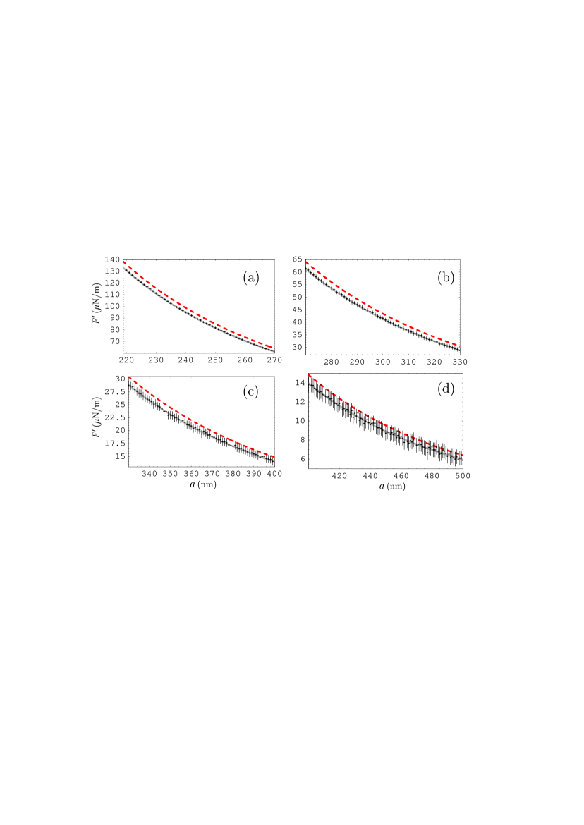
Figure 4: (Color online) Comparison between the experimental data for the gradient of the Casimir force (crosses) and theory (solid and dashed bands computed using the plasma model approach with included and omitted magnetic properties of Ni plate, respectively).

References

- (1) H. B. G. Casimir, Proc. K. Ned. Akad. Wet. B 51, 793 (1948).
- (2) K. A. Milton, The Casimir Effect (World Scientific, Singapore, 2001).
- (3) M. Bordag, G. L. Klimchitskaya, U. Mohideen, and V. M. Mostepanenko, Advances in the Casimir Effect (Oxford University Press, Oxford, 2009).
- (4) G. L. Klimchitskaya, U. Mohideen, and V. M. Mostepanenko, Rev. Mod. Phys. 81, 1827 (2009).
- (5) A. W. Rodriguez, F. Capasso, and S. G. Johnson, Nature Photon. 5, 211 (2011).
- (6) G. L. Klimchitskaya, U. Mohideen, and V. M. Mostepanenko, Int. J. Mod. Phys. B 25, 171 (2011).
- (7) E. M. Lifshitz, Zh. Eksp. Teor. Fiz. 29, 94 (1955) [Sov. Phys. JETP 2, 73 (1956)].
- (8) T. Emig, R. L. Jaffe, M. Kardar, and A. Scardicchio, Phys. Rev. Lett. 96, 080403 (2006).
- (9) T. Emig, N. Graham, R. L. Jaffe, and M. Kardar, Phys. Rev. Lett. 99, 017403 (2007).
- (10) O. Kenneth and I. Klich, Phys. Rev. B 78, 014103 (2008).
- (11) M. Boström and B. E. Sernelius, Phys. Rev. Lett. 84, 4757 (2000).
- (12) I. Brevik, J. B. Aarseth, J. S. Høye, and K. A. Milton, Phys. Rev. E 71, 056101 (2005).
- (13) M. Bordag, B. Geyer, G. L. Klimchitskaya, and V. M. Mostepanenko, Phys. Rev. Lett. 85, 503 (2000).
- (14) C. Genet, A. Lambrecht, and S. Reynaud, Phys. Rev. A 62, 012110 (2000).
- (15) R. S. Decca, D. López, E. Fischbach, G. L. Klimchitskaya, D. E. Krause, and V. M. Mostepanenko, Ann. Phys. (N.Y.) 318, 37 (2005); Phys. Rev. D 75, 077101 (2007); Eur. Phys. J. C 51, 963 (2007).
- (16) C.-C. Chang, A. A. Banishev, R. Castillo-Garza, G. L. Klimchitskaya, V. M. Mostepanenko, and U. Mohideen, Phys. Rev. B 85, 165443 (2012).
- (17) A. O. Sushkov, W. J. Kim, D. A. R. Dalvit, and S. K. Lamoreaux, Nature Phys. 7, 230 (2011).
- (18) V. B. Bezerra, G. L. Klimchitskaya, U. Mohideen, V. M. Mostepanenko, and C. Romero, Phys. Rev. B 83, 075417 (2011).
- (19) G. L. Klimchitskaya, M. Bordag, E. Fischbach, D. E. Krause, and V. M. Mostepanenko, Int. J. Mod. Phys. A 26, 3918 (2011).
- (20) F. Chen, G. L. Klimchitskaya, V. M. Mostepanenko, and U. Mohideen, Optics Express 15, 4823 (2007); Phys. Rev. B 76, 035338 (2007).
- (21) C.-C. Chang, A. A. Banishev, G. L. Klimchitskaya, V. M. Mostepanenko, and U. Mohideen, Phys. Rev. Lett. 107, 090403 (2011).
- (22) A. A. Banishev, C.-C. Chang, R. Castillo-Garza, G. L. Klimchitskaya, V. M. Mostepanenko, and U. Mohideen, Phys. Rev. B 85, 045436 (2012).
- (23) J. M. Obrecht, R. J. Wild, M. Antezza, L. P. Pitaevskii, S. Stringari, and E. A. Cornell, Phys. Rev. Lett. 98, 063201 (2007).
- (24) G. L. Klimchitskaya and V. M. Mostepanenko, J. Phys. A: Math. Theor. 41, 312002(F) (2008).
- (25) P. Richmond and B. W. Ninham, J. Phys. C: Solid St. Phys. 4, 1988 (1971).
- (26) S. Y. Buhmann, D.-G. Welsch, and T. Kampf, Phys. Rev. A 72, 032112 (2005).
- (27) M. S. Tomaš, Phys. Lett. A 342, 381 (2005).
- (28) S. J. Rahi, T. Emig, N. Graham, R. L. Jaffe, and M. Kardar, Phys. Rev. D 80, 085021 (2009).
- (29) Yu. S. Barash and V. L. Ginzburg, Usp. Fiz. Nauk 116, 5 (1975) [Sov. Phys. Usp. 18, 305 (1975)].
- (30) O. Kenneth, I. Klich, A. Mann, and M. Revzen, Phys. Rev. Lett. 89, 033001 (2002).
- (31) D. Iannuzzi and F. Capasso, Phys. Rev. Lett. 91, 029101 (2003).
- (32) F. S. S. Rosa, D. A. R. Dalvit, and P. W. Milonni, Phys. Rev. A 78, 032117 (2008).
- (33) N. Inui, Phys. Rev. A 83, 032513 (2011); Phys. Rev. A 84, 052505 (2011).
- (34) B. Geyer, G. L. Klimchitskaya, and V. M. Mostepanenko, Phys. Rev. B 81, 104101 (2010); G. L. Klimchitskaya, B. Geyer, and V. M. Mostepanenko, Int. J. Mod. Phys. A 25, 2293 (2010).
- (35) S. de Man, K. Heeck, R. J. Wijngaarden, and D. Iannuzzi, Phys. Rev. Lett. 103, 040402 (2009).
- (36) G. Torricelli, P. J. van Zwol, O. Shpak, C. Binns, G. Palasantzas, B. J. Kooi, V. B. Svetovoy, and M. Wuttig, Phys. Rev. A 82, 010101(R) (2010).
- (37) T. R. Albrecht, P. Grütter, D. Horne, and D. Rugar, J. Appl. Phys. 69, 668 (1991).
- (38) G. Jourdan. A. Lambrecht, F. Comin, and J. Chevrier, Europhys. Lett. 85, 31001 (2009).
- (39) F. Chen and U. Mohideen, Rev. Sci. Instrum. 72, 3100 (2001).
- (40) G. Bimonte, T. Emig, R. L. Jaffe, and M. Kardar, Europhys. Lett. 97, 50001 (2012).
- (41) G. Bimonte, T. Emig, and M. Kardar, Appl. Phys. Lett. 100, 074110 (2012).
- (42) Handbook of Optical Constants of Solids, ed. E. D. Palik (Academic, New York, 1985).
- (43) M. A. Ordal, R. J. Bell, R. W. Alexander Jr., L. L. Long, and M. R. Querry, Appl. Opt. 24, 4493 (1985).