Discriminating $Z^{\prime}$ from anomalous trilinear gauge coupling signatures in $e^{+}e^{-}\rightarrow W^{+}W^{-}$ at ILC with polarized beams

Abstract

New heavy neutral gauge bosons $Z^{\prime}$ are predicted by many models of physics beyond the Standard Model. It is quite possible that $Z^{\prime}$s are heavy enough to lie beyond the discovery reach of the CERN Large Hadron Collider LHC, in which case only indirect signatures of $Z^{\prime}$ exchanges may emerge at future colliders, through deviations of the measured cross sections from the Standard Model predictions. We discuss in this context the foreseeable sensitivity to $Z^{\prime}$s of $W^{\pm}$-pair production cross sections at the $e^{+}e^{-}$ International Linear Collider (ILC), especially as regards the potential of distinguishing observable effects of the $Z^{\prime}$ from analogous ones due to competitor models with anomalous trilinear gauge couplings (AGC) that can lead to the same or similar new physics experimental signatures at the ILC. The sensitivity of the ILC for probing the $Z$-$Z^{\prime}$ mixing and its capability to distinguish these two new physics scenarios is substantially enhanced when the polarization of the initial beams and the produced $W^{\pm}$ bosons are considered. A model independent analysis of the $Z^{\prime}$ effects in the process $e^{+}e^{-}\rightarrow W^{+}W^{-}$ allows to differentiate the full class of vector $Z^{\prime}$ models from those with anomalous trilinear gauge couplings, with one notable exception: the sequential SM (SSM)-like models can in this process not be distinguished from anomalous gauge couplings. Results of model dependent analysis of a specific $Z^{\prime}$ are expressed in terms of discovery and identification reaches on the $Z$-$Z^{\prime}$ mixing angle and the $Z^{\prime}$ mass.

I Introduction

The $W^{\pm}$ boson pair production process

$$e^{+}+e^{-}\rightarrow W^{+}+W^{-}$$ (1)

is a crucial one for studying the electroweak gauge symmetry in $e^{+}e^{-}$ annihilation. Properties of the weak gauge bosons are closely related to electroweak symmetry breaking and the structure of the gauge sector in general. Thus, detailed examination of (1) at the ILC will both test this sector of the standard model (SM) with the highest accuracy and throw light on New Physics (NP) that may appear beyond the SM.

In the SM, for zero electron mass, the process (1) is described by the amplitudes mediated by photon and $Z$ boson exchange in the $s$-channel and by neutrino exchange in the $t$-channel. Therefore, this reaction is particularly sensitive to both the leptonic vertices and the trilinear couplings to $W^{+}W^{-}$ of the SM $Z$ and of any new heavy neutral boson that can be exchanged in the $s$-channel. A popular example in this regard, is represented by the $Z^{\prime}$s envisaged by electroweak scenarios based on spontaneously broken ‘extended’ gauge symmetries, with masses much larger than $M_{Z}$ and coupling constants different from the SM. The variety of the proposed $Z^{\prime}$ models is broad. Therefore, rather than attempting an exhaustive analysis, we shall here focus on the phenomenological effects in reaction (1) of the so-called $Z^{\prime}_{\rm SSM}$, $Z^{\prime}_{E_{6}}$ and $Z^{\prime}_{\rm LR}$ models. Actually, in some sense, we may consider these $Z^{\prime}$ models as representative of this New Physics (NP) sector Langacker:2008yv ; Rizzo:2006nw ; Leike:1996pj ; Leike:1998wr ; Hewett:1988xc ; Erler:2009jh ; Langacker:2009su ; Riemann:2005es .

The direct manifestation of $Z^{\prime}$s would be the observation of peaks in cross sections at very high energy colliders, this would be possible only for $M_{Z^{\prime}}$ lying within the kinematical reach of the machine and sufficient luminosity. Indeed, current lower limits on $M_{Z^{\prime}}$ are obtained from direct searches of $Z^{\prime}$s in Drell-Yan dilepton pair production at the CERN LHC: from the analysis of the 7 TeV data, the observed bounds at 95% C. L. range approximately in the interval $1.8-2.3~{}\text{TeV}$, depending on the particular $Z^{\prime}$ model being tested Chatrchyan:2012it ; atlas-dilepton . For too high masses, $Z^{\prime}$ exchanges can manifest themselves indirectly, via deviations of cross sections, and in general of the reaction observables, from the SM predictions. Clearly, this kind of searches requires great precision and therefore will be favoured by extremely high collider luminosity, such as will be available at the ILC. Indirect lower bounds on $Z^{\prime}$ masses from the high precision LEP data at the $Z$ lie in the range $\sim 0.4-1.8~{}\text{TeV}$, depending on the model considered Erler:2009jh ; Langacker:2009su .

Indirect effects may be quite subtle, as far as the identification of the source of an observed deviation is concerned, because a priori different NP scenarios may lead to the same or similar experimental signatures. Clearly, then, the discrimination of one NP model (in our case the $Z^{\prime}$) from other possible ones needs an appropriate strategy for analyzing the data.

In this paper, we study the indirect effects evidencing the mentioned extra $Z^{\prime}$ gauge bosons in $W^{\pm}$ pair production (1) at the next generation $e^{+}e^{-}$ International Linear Collider (ILC), with a center of mass energy $\sqrt{s}=0.5-1~{}\text{TeV}$ and typical time-integrated luminosities of ${\cal L}_{\rm int}\sim 0.5-1$ ab^-1 :2007sg ; Djouadi:2007ik . At the foreseen, really high luminosity this process should be quite sensitive to the indirect NP effects at a collider with $M_{Z}\ll\sqrt{s}\ll M_{Z^{\prime}}$ Pankov:1990hq ; Pankov:1992cy ; Pankov:1994hx ; Pankov:1997da ; Jung:1999wq ; Ananthanarayan:2010bt , the deviations of cross sections from the SM predictions being expected to increase with $\sqrt{s}$ due to the violation of the SM gauge cancellation among the different contributions.

Along the lines of the previous discussion, apart from estimating the foreseeable sensitivity of process (1) to the considered $Z^{\prime}$ models, we will consider the problem of establishing the potential of ILC of distinguishing the $Z^{\prime}$ effects, once observed, from the ones due to NP competitor models that can lead to analogous physical signatures in the cross section. For the latter, we will choose the models with Anomalous Gauge Couplings (AGC), and compare them with the hypothesis of $Z^{\prime}$ exchanges. In the AGC models, there is no new gauge boson exchange, but the $WW\gamma$, $WWZ$ couplings are modified with respect to the SM values, this violates the SM gauge cancellation too and leads to deviations of the process cross sections. AGC couplings are described via a sum of effective interactions, ordered by dimensionality, and we shall restrict our analysis to the dimension-six terms which conserve $C$ and $P$ gounaris ; Gounaris:1992kp .

The baseline configuration of the ILC envisages a very high electron beam polarization (larger than 80%) that is measurable with high precision. Also positron beam polarization, around 30%, might be initially obtainable, and this polarization could be raised to about 60% or higher in the ultimate upgrade of the machine. As is well-known, the polarization option represents an asset in order to enhance the discovery reaches and identification sensitivities on NP models of any kind MoortgatPick:2005cw ; Osland:2009dp . This is the case, in particular, of $Z^{\prime}$ exchanges and AGC interactions in process (1), an obvious example being the suppression of the $\nu$-exchange channel by using right-handed electrons. Additional ILC diagnostic ability in $Z^{\prime}$s and AGC would be provided by measures of polarized $W^{+}$ and $W^{-}$ in combination with initial beam polarizations.

The paper is organized as follows. In Section II, we briefly review the models involving additional $Z^{\prime}$ bosons and emphasize the role of $Z$-$Z^{\prime}$ mixing in the process (1). In Section III we give the parametrization of $Z^{\prime}$ and AGC effects, as well as formulae for helicity amplitudes and cross sections of the process under consideration. Section IV contains, for illustrative purposes, some plots of the unpolarized and polarized cross sections showing the effect of $Z^{\prime}$ and of $Z$-$Z^{\prime}$ mixing. In Section V we present the approach, which allows to obtain the discovery reach on $Z^{\prime}$ parameters (actually, on the deviations of the transition amplitudes from the SM) and the obtained numerical results. Section VI includes the results of both model dependent and model independent analyses of the possibilities to differentiate $Z^{\prime}$ effects from similar ones caused by AGC. Finally we conclude in Section VII.

II $Z^{\prime}$ models and $Z$-$Z^{\prime}$ mixing

The $Z^{\prime}$ models that will be considered in our analysis are the following Langacker:2008yv ; Rizzo:2006nw ; Leike:1998wr ; Hewett:1988xc :

• The four possible $U(1)$ $Z^{\prime}$ scenarios originating from the spontaneous breaking of the exceptional group $E_{6}$. In this case, two extra, heavy neutral gauge bosons appear as consequence of the symmetry breaking and, generally, only the lightest is assumed to be within reach of the collider. It is defined, in terms of a new mixing angle $\beta$, by the linear combination

  $$Z^{\prime}=Z^{\prime}_{\chi}\cos\beta+Z^{\prime}_{\psi}\sin\beta.$$ (2)

  Specific choices of $\beta$: $\beta=0$; $\beta=\pi/2$; $\beta=-\arctan{\sqrt{5/3}}$ and $\beta=\arctan{\sqrt{3/5}}$, corresponding to different $E_{6}$ breaking patterns, define the popular scenarios $Z^{\prime}_{\chi}$, $Z^{\prime}_{\psi}$, $Z^{\prime}_{\eta}$ and $Z^{\prime}_{I}$, respectively.

• The left-right models, originating from the breaking down of an $SO(10)$ grand-unification symmetry, and where the corresponding $Z^{\prime}_{\rm LR}$ couple to a linear combination of right-handed and $B-L$ neutral currents ($B$ and $L$ being baryon and lepton numbers, respectively):

  $$J^{\mu}_{\rm LR}=\alpha_{\rm LR}J^{\mu}_{3R}-\frac{1}{2\alpha_{\rm LR}}J^{\mu}_{B-L}\quad{\rm with}\quad\alpha_{\rm LR}={\sqrt{\frac{c_{W}^{2}}{s_{W}^{2}}\,\kappa^{2}-1}}.$$ (3)

  Here, $s_{W}=\sin\theta_{W}$, $c_{W}=\sqrt{1-s_{W}^{2}}$, additional parameters are the ratio $\kappa=g_{\rm R}/g_{\rm L}$ of the $SU(2)_{\rm L,R}$ gauge couplings and $\alpha_{\rm LR}$, restricted to the range $\sqrt{2/3}\lesssim\alpha_{\rm LR}\lesssim 1.52$. The upper bound corresponds to the so-called LR-symmetric $Z^{\prime}_{\rm LRS}$ model with $g_{\rm R}=g_{\rm L}$, while the lower bound is found to coincide with the $Z^{\prime}_{\chi}$ model introduced above. We will consider the former one, $Z^{\prime}_{\rm LRS}$, throughout the paper.

• The $Z^{\prime}_{\rm ALR}$ predicted by the so-called ‘alternative’ left-right scenario. For the LR model we need not introduce additional fermions to cancel anomalies. However, in the $E_{6}$ case a variant of this model (called the Alternative LR model) can be constructed by altering the embeddings of the SM and introducing exotic fermions into the ordinary 10 and 5 representations.

• The so-called sequential $Z^{\prime}_{\text{SSM}}$, where the couplings to fermions are the same as those of the SM $Z$.

Detailed descriptions of these models, as well as the specific references, can be found, e. g., in Refs. Langacker:2008yv ; Rizzo:2006nw ; Leike:1998wr ; Hewett:1988xc .

In the extended gauge theories predicting the existence of an extra neutral $Z^{\prime}$ gauge boson, the mass-squared matrix of the $Z$ and $Z^{\prime}$ can have non-diagonal entries $\delta M^{2}$, which are related to the vacuum expectation values of the fields of an extended Higgs sector Leike:1998wr :

$$M_{ZZ^{\prime}}^{2}=\left(\begin{matrix}M_{Z}^{2}&\delta M^{2}\\ \delta M^{2}&M_{Z^{\prime}}^{2}\end{matrix}\right).$$ (4)

Here, $Z$ and $Z^{\prime}$ denote the weak gauge boson eigenstates of $SU(2)_{L}\times U(1)_{Y}$ and of the extra $U(1)^{\prime}$, respectively. The mass eigenstates, $Z_{1}$ and $Z_{2}$, diagonalizing the matrix (4), are then obtained by the rotation of the fields $Z$ and $Z^{\prime}$ by a mixing angle $\phi$:

$$Z_{1}=Z\cos\phi+Z^{\prime}\sin\phi\;,$$ (5)

$$Z_{2}=-Z\sin\phi+Z^{\prime}\cos\phi\;.$$ (6)

Here, the mixing angle $\phi$ is expressed in terms of masses as:

$$\tan^{2}\phi={\frac{M_{Z}^{2}-M_{1}^{2}}{M_{2}^{2}-M_{Z}^{2}}}\simeq\frac{2M_{Z}\Delta M}{M_{2}^{2}}\;,$$ (7)

where $\Delta M=M_{Z}-M_{1}>0$, $M_{Z}$ is the mass of the $Z_{1}$-boson in the absence of mixing, i.e., for $\phi=0$. Once we assume the mass $M_{1}$ to be determined experimentally, the mixing depends on two free parameters, which we identify as $\phi$ and $M_{2}$. We shall here consider the configuration $M_{1}\ll\sqrt{s}\ll M_{2}$.

The mixing angle $\phi$ will play an important role in our analysis. In general, such mixing effects reflect the underlying gauge symmetry and/or the Higgs sector of the model. To a good approximation, for $M_{1}\ll M_{2}$, in specific “minimal-Higgs models” UPR-0476T ,

$$\phi\simeq-s^{2}_{\mathrm{W}}\ \frac{\sum_{i}\langle\Phi_{i}\rangle{}^{2}I^{i}_{3L}Q^{\prime}_{i}}{\sum_{i}\langle\Phi_{i}\rangle^{2}(I^{i}_{3L})^{2}}={\cal C}\ {\frac{\displaystyle M^{2}_{1}}{\displaystyle M^{2}_{2}}}.$$ (8)

Here $\langle\Phi_{i}\rangle$ are the Higgs vacuum expectation values spontaneously breaking the symmetry, and $Q^{\prime}_{i}$ are their charges with respect to the additional $U(1)^{\prime}$. In addition, in these models the same Higgs multiplets are responsible for both generation of mass $M_{1}$ and for the strength of the $Z$-$Z^{\prime}$ mixing Langacker:2008yv . Thus ${\cal C}$ is a model-dependent constant. For example, in the case of $E_{6}$ superstring-inspired models ${\cal C}$ can be expressed as UPR-0476T

$${\cal C}=4s_{\mathrm{W}}\left(A-\frac{\sigma-1}{\sigma+1}B\right),$$ (9)

where $\sigma$ is the ratio of vacuum expectation values squared, and the constants $A$ and $B$ are determined by the mixing angle $\beta$: $A=\cos\beta/2\sqrt{6}$, $B=\sqrt{10}/12\sin\beta$.

An important property of the models under consideration is that the gauge eigenstate $Z^{\prime}$ does not couple to the $W^{+}W^{-}$ pair since it is neutral under $SU(2)_{L}$. Therefore the process (1), and the searched-for deviations of the cross sections from the SM, are sensitive to a $Z^{\prime}$ only in the case of a non-zero $Z$-$Z^{\prime}$ mixing. The mixing angle is rather highly constrained, to an upper limit of $\text{a few}\times 10^{-3}$, mainly from LEP measurements at the $Z$ Erler:2009jh ; Langacker:2009su . The high statistics on $W$-pair production expected at the ILC might in principle allow to probe such small mixing angles effectively.

From (5) and (6), one obtains the vector and axial-vector couplings of the $Z_{1}$ and $Z_{2}$ bosons to fermions:

$$v_{1f}=v_{f}\cos\phi+v_{f}^{\prime}\sin\phi\;,\;\;\;a_{1f}=a_{f}\cos\phi+a_{f}^{\prime}\sin\phi\;,$$ (10)

$$v_{2f}=-v_{f}\sin\phi+v_{f}^{\prime}\cos\phi\;,\;\;\;a_{2f}=-a_{f}\sin\phi+a_{f}^{\prime}\cos\phi,$$ (11)

with $(v_{f},a_{f})=(g^{f}_{L}\pm g^{f}_{R})/2$, and $(v_{f}^{\prime},a_{f}^{\prime})$ similarly defined in terms of the $Z^{\prime}$ couplings. The fermonic $Z^{\prime}$ couplings can be found in Langacker:2008yv ; Rizzo:2006nw ; Leike:1998wr ; Hewett:1988xc .

Analogously, one obtains according to the remarks above:

$$g_{WWZ_{1}}=\cos\phi\;g_{WWZ}\;,$$ (12)

$$g_{WWZ_{2}}=-\sin\phi\;g_{WWZ}\;,$$ (13)

where $g_{WWZ}=\cot\theta_{W}$.

III Parameterizations of $Z^{\prime}$-boson and AGC effects

III.1 $Z^{\prime}$ boson

The starting point of our analysis will be the amplitude for the process (1). In the Born approximation, this can be written as a sum of a $t$-channel and an $s$-channel component. In the SM case, the latter will be schematically written as follows:

$${\cal M}_{s}^{(\lambda)}=\left(-\frac{1}{s}+\frac{\cot\theta_{W}(v-2\lambda a)}{s-M^{2}_{Z}}\right)\times{\cal G}^{(\lambda)}(s,\theta),$$ (14)

where $s$ and $\theta$ are the total c.m. squared energy and $W^{-}$ production angle. Omitting the fermion subscripts, electron vector and axial-vector couplings in the SM are denoted as $v=(T_{3,e}-2Q_{e}\hskip 2.0pts_{W}^{2})/2s_{W}c_{W}$ and $a=T_{3,e}/2s_{W}c_{W}$, respectively, with $T_{3,e}=-1/2$, and $\lambda$ denoting the electron helicity ($\lambda=\pm 1/2$ for right/left-handed electrons). Finally, ${\cal G}^{(\lambda)}(s,\theta)$ is a kinematical coefficient, depending also on the $W^{\pm}$ helicities. The explicit form can be found in the literature gounaris ; Gounaris:1992kp or derived from the entries of Table 5, which also shows the form of the $t$-channel neutrino exchange.

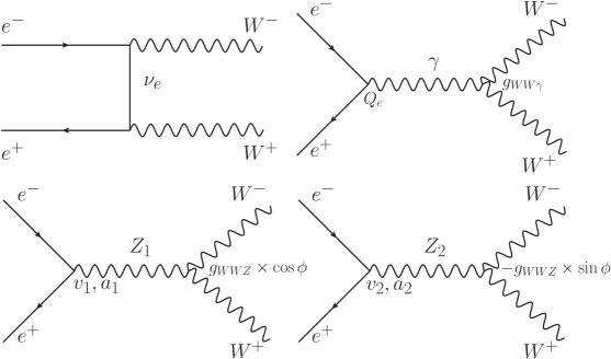
Figure 1: Feynman diagrams for the process $e^{-}e^{+}\rightarrow W^{-}W^{+}$ in the Born approximation

In the extended gauge models the process (1) is described by the set of diagrams displayed in Fig. 1. The amplitude with the extra $Z^{\prime}$ depicted in Fig. 1 will be written as:

$${\cal M}_{s}^{(\lambda)}=\left(-\frac{1}{s}+\frac{g_{WWZ_{1}}(v_{1}-2\lambda a_{1})}{s-M_{1}^{2}}+\frac{g_{WWZ_{2}}(v_{2}-2\lambda a_{2})}{s-M_{2}^{2}}\right)\times{\cal G}^{(\lambda)}(s,\theta).$$ (15)

The contribution of the new heavy neutral gauge boson $Z_{2}$ to the amplitude of process (1) is represented by the fourth diagram in Fig. 1. In addition, there are indirect contributions to the $Z_{1}$-mediated diagram, represented by modifications of the electron and three-boson vertices induced by the $Z$-$Z^{\prime}$ mixing.

It is convenient to rewrite Eq. (15) in the following form Pankov:1997da :

$${\cal M}_{s}^{(\lambda)}=\left(-\frac{g_{WW\gamma}}{s}+\frac{g_{WWZ}(v-2\lambda a)}{s-M^{2}_{Z}}\right)\times{\cal G}^{(\lambda)}(s,\theta),$$ (16)

where the ‘effective’ gauge boson couplings $g_{WW\gamma}$ and $g_{WWZ}$ are defined as:

$$g_{WW\gamma}=1+\Delta_{\gamma}=1+\Delta_{\gamma}(Z_{1})+\Delta_{\gamma}(Z_{2}),$$ (17)

$$g_{WWZ}=\cot\theta_{W}+\Delta_{Z}=\cot\theta_{W}+\Delta_{Z}(Z_{1})+\Delta_{Z}(Z_{2}),$$ (18)

with

$$\Delta_{\gamma}(Z_{1})=v\hskip 2.0pt\cot\theta_{W}\hskip 2.0pt\left(\frac{\Delta a}{a}-\frac{\Delta v}{v}\right)\hskip 1.0pt\left(1+\Delta\chi\right)\hskip 1.0pt\chi;\ \ \Delta_{\gamma}(Z_{2})=v\hskip 2.0ptg_{WWZ_{2}}\hskip 2.0pt\left(\frac{a_{2}}{a}-\frac{v_{2}}{v}\right)\hskip 2.0pt\chi_{2},$$ (19)

$$\Delta_{Z}(Z_{1})=\Delta g_{WWZ}+\cot\theta_{W}\hskip 1.0pt\left(\frac{\Delta a}{a}+\Delta\chi\right);\qquad\Delta_{Z}(Z_{2})=g_{WWZ_{2}}\hskip 2.0pt\frac{a_{2}}{a}\hskip 2.0pt\frac{\chi_{2}}{\chi}.$$ (20)

In Eqs. (19) and (20) we have introduced the deviations of the fermionic and trilinear bosonic couplings $\Delta v=v_{1}-v$, $\Delta a=a_{1}-a$ and $\Delta g_{WWZ}=g_{WWZ_{1}}-\cot\theta_{W}$, and the neutral vector boson propagators (neglecting their widths):

$$\chi(s)=\frac{s}{s-M^{2}_{Z}};\qquad\chi_{2}(s)=\frac{s}{s-M^{2}_{2}};\qquad\Delta\chi(s)\simeq-\frac{2M_{Z}\Delta M}{s-M^{2}_{Z}},$$ (21)

where $\Delta M=M_{Z}-M_{1}$ is the $Z$-$Z_{1}$ mass shift. Because $W$ pair production is studied sufficiently far away from the $Z_{1}$ peak, we can neglect the $Z$ and $Z_{1,2}$ widths in (15) and (16).

It should be stressed that, not referring to specific models, the parametrization (16)-(18) is both general and useful for phenomenological purposes, in particular to compare different sources of nonstandard effects contributing finite deviations (19) and (20) to the SM predictions. Note that $\Delta_{\gamma}$ vanishes as $s\rightarrow 0$, consistent with gauge invariance.

We know from current measurements Erler:2009jh that $\Delta M<100$ MeV. This allows the approximation $\Delta\chi(s)\ll 1$. One can rewrite (19) and (20) in a simplified form taking into account the approximation above as well as the couplings to first order in $\phi$ as:

$$(v_{1},\hskip 1.0pta_{1})\simeq(v+v^{\prime}\hskip 1.0pt\phi,\hskip 1.0pta+a^{\prime}\hskip 1.0pt\phi)\Rightarrow(\Delta v,\hskip 1.0pt\Delta a)\simeq(v^{\prime}\hskip 1.0pt\phi,a^{\prime}\hskip 1.0pt\phi),$$ (22)

$$(v_{2},\hskip 1.0pta_{2})\simeq(-v\hskip 1.0pt\phi+v^{\prime},\hskip 1.0pt-a\hskip 1.0pt\phi+a^{\prime}),$$ (23)

and

$$g_{WWZ_{1}}\simeq g_{WWZ};\qquad\quad g_{WWZ_{2}}\simeq-g_{WWZ}\hskip 1.0pt\phi.$$ (24)

In the case of extended models considered here, e.g. $E_{6}$, $v^{\prime}$ and $a^{\prime}$ are explicitly parametrized in terms of the angle $\beta$ which characterizes the direction of the $Z^{\prime}$-related extra $U(1)^{\prime}$ generator in the $E_{6}$ group space, and reflects the pattern of symmetry breaking to $SU(2)_{L}\times U(1)_{Y}$ Langacker:2008yv ; Rizzo:2006nw ; Leike:1998wr ; Hewett:1988xc :

$$v^{\prime}=\frac{\cos\beta}{c_{W}\hskip 1.0pt\sqrt{6}};\qquad\quad a^{\prime}=\frac{1}{2\hskip 1.0ptc_{W}\sqrt{6}}\left(\cos\beta+\sqrt{\frac{5}{3}}\sin\beta\right).$$ (25)

Substituting Eqs. (22)–(24) into (19) and (20), one finds the general form of $\Delta_{\gamma}$ and $\Delta_{Z}$:

$$\Delta_{\gamma}=\phi\cdot v\hskip 2.0pt\cot\theta_{W}\hskip 2.0pt\left(\frac{a^{\prime}}{a}-\frac{v^{\prime}}{v}\right)\left(1-\frac{\chi_{2}}{\chi}\right)\chi,$$ (26)

$$\Delta_{Z}=\phi\cdot\hskip 2.0pt\cot\theta_{W}\hskip 2.0pt\frac{a^{\prime}}{a}\left(1-\frac{\chi_{2}}{\chi}\right).$$ (27)

Both these quantities have the same dependence on $\phi$ and $M_{2}$, via the product $\phi(1-\chi_{2}/\chi)$. Thus, $\phi$ and $M_{2}$ can not be separately determined from a measurement of $\Delta_{\gamma}$ and $\Delta_{Z}$, only this composite function can be determined. We also note that for an SSM-type model, the first parenthesis in Eq. (26) vanishes, resulting in $\Delta_{\gamma}=0$. Thus, these models can not be distinguished from the AGC models, introduced in the next section. Further, the terms proportional to $\chi_{2}$ in Eqs. (26) and (27) dominate in the case $\sqrt{s}\approx M_{2}$ but will be very small in the case $\sqrt{s}\ll M_{2}$.

III.2 Anomalous Gauge Couplings

As pointed out in the Introduction, a model with an extra $Z^{\prime}$ would produce virtual manifestations in the final $W^{+}W^{-}$ channel at the ILC that in principle could mimic those of a model with AGC, hence of completely different origin. This is due to the fact that, as shown above, the effects of the extra $Z^{\prime}$ can be reabsorbed into a redefinition of the $WWV$ couplings ($V=\gamma,\hskip 2.0ptZ$). Therefore, the identification of such an effect, if observed at the ILC, becomes a very important problem Hagiwara:1986vm .

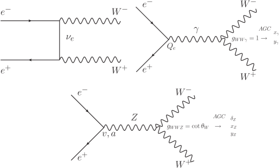
Figure 2: Feynman diagrams for the process $e^{+}e^{-}\rightarrow W^{+}W^{-}$ in the Standard Model and with anomalous trilinear gauge couplings (AGC).

Using the notations of, e.g., Ref. gounaris ; Gounaris:1992kp , the relevant trilinear $WWV$ interaction up to operators of dimension-6, which conserves $U(1)_{\text{e.m.}}$, $C$ and $P$, can be written as ($e=\sqrt{4\pi\alpha_{em}}$):

$${\cal L}_{\text{eff}} = -ie\left[A_{\mu}\left(W^{-\mu\nu}W^{+}_{\nu}-W^{+\mu\nu}W^{-}_{\nu}\right)+F_{\mu\nu}W^{+\mu}W^{-\nu}\right]$$ (28)

$$- ie\hskip 2.0pt\left(\cot\theta_{W}+\delta_{Z}\right)\hskip 2.0pt\left[Z_{\mu}\left(W^{-\mu\nu}W^{+}_{\nu}-W^{+\mu\nu}W^{-}_{\nu}\right)+Z_{\mu\nu}W^{+\mu}W^{-\nu}\right]$$

$$- ie\hskip 2.0ptx_{\gamma}\hskip 2.0ptF_{\mu\nu}W^{+\mu}W^{-\nu}-ie\hskip 2.0ptx_{Z}\hskip 2.0ptZ_{\mu\nu}W^{+\mu}W^{-\nu}$$

$$+ ie\hskip 2.0pt\frac{y_{\gamma}}{M_{W}^{2}}\hskip 2.0ptF^{\nu\lambda}W^{-}_{\lambda\mu}W^{+\mu}_{\ \ \nu}+ie\hskip 2.0pt\frac{y_{Z}}{M_{W}^{2}}\hskip 2.0ptZ^{\nu\lambda}W^{-}_{\lambda\mu}W^{+\mu}_{\ \ \nu}\hskip 2.0pt,$$

where $W_{\mu\nu}^{\pm}=\partial_{\mu}W_{\nu}^{\pm}-\partial_{\nu}W_{\mu}^{\pm}$ and ${Z_{\mu\nu}=\partial_{\mu}Z_{\nu}-\partial_{\nu}Z_{\mu}}$. In the SM at the tree-level, the anomalous couplings in (28) vanish: $\delta_{Z}=x_{\gamma}=x_{Z}=y_{\gamma}=y_{Z}=0$.

The anomalous gauge couplings are here parametrized in terms of five real independent parameters. This number can be reduced by imposing additional constraints, like local $SU(2)_{L}\times U(1)_{Y}$ symmetry, in which case the number would be reduced to three (see for example Tables 2 and 1 of Bilenky:1993ms and Bilenky:1993uy , respectively).

Current limits reported by the Particle Data Group Nakamura:2010zzi , that show the sensitivity to the AGCs attained so far, are roughly of the order of 0.04 for $\delta_{Z}$, 0.05 for $x_{\gamma}$, 0.02 for $y_{\gamma}$, 0.11 for $x_{Z}$ and 0.12 for $y_{Z}$. As will be shown in the next sections, at the ILC in the energy and luminosity configuration considered here, sensitivities to deviations from the SM, hence of indirect New Physics signatures, down to the order of $10^{-3}$ will be reached. This would compare with the expected order of magnitude of the theoretical uncertainty on the SM cross sections after accounting for higher-order corrections to the Born amplitudes of Figs. 1 and 2, formally of order $\alpha_{\text{em}}$ Fleischer:1991nw ; Beenakker:1994vn , but that for distributions can reach the size of 10%, depending on $\sqrt{s}$ Denner:2005es ; Denner:2005fg .

III.3 Helicity amplitudes and cross sections

The general expression for the cross section of process (1) with longitudinally polarized electron and positron beams described by the set of diagrams presented in Fig. 2 can be expressed as

$$\frac{d\sigma}{d\cos\theta}=\frac{1}{4}\left[\left(1+P_{L}\right)\left(1-{\bar{P}}_{L}\right)\frac{d\sigma^{+}}{d\cos\theta}+\left(1-P_{L}\right)\left(1+{\bar{P}}_{L}\right)\frac{d\sigma^{-}}{d\cos\theta}\right],$$ (29)

where $P_{L}$ and ${\bar{P}}_{L}$ are the actual degrees of electron and positron longitudinal polarization, respectively, and $\sigma^{\pm}$ are the cross sections for purely right-handed ($\lambda=1/2$) and left-handed ($\lambda=-1/2$) electrons. From Eq. (29), the cross section for polarized (unpolarized) electrons and unpolarized positrons corresponds to $P_{L}\neq 0$ and ${\bar{P}_{L}}=0$ ($P_{L}={\bar{P}_{L}}=0$).

The polarized cross sections can generally be written as follows:

$$\frac{d\sigma^{\pm}}{d\hskip 1.0pt\cos\theta}=\frac{|{\bf p}|}{16\pi s\sqrt{s}}\sum_{\tau,\tau^{\prime}}|F_{\lambda\tau\tau^{\prime}}(s,\cos\theta)|^{2}.$$ (30)

Here, the helicities of the $W^{-}$ and $W^{+}$ are denoted by $\tau,\tau^{\prime}=\pm 1,0$. Corresponding to the interaction (28), the helicity amplitudes $F_{\lambda\tau\tau^{\prime}}(s,\cos\theta)$ have the structure shown in Table 5 gounaris ; Gounaris:1992kp in Appendix A. In Table 5, $\beta_{W}=\sqrt{1-4M_{W}^{2}/s}=2p/\sqrt{s}$, with $p=|\bm{p}|$ the c.m. momentum of the $W^{-}$. Furthermore, $s$ and $t$ are the Mandelstam variables, and $\theta$ the c.m. scattering angle, with $t=M_{W}^{2}-s(1-\beta\cos\theta)/2$. For comparison, we also show in Appendix A the corresponding helicity amplitudes for the case of a $Z^{\prime}$.

We define the differential cross sections for correlated spins of the produced $W^{-}$ and $W^{+}$,

$$\frac{d\sigma(W^{+}_{L}W^{-}_{L})}{d\cos\theta},\qquad\frac{d\sigma(W^{+}_{T}W^{-}_{T})}{d\cos\theta},\qquad\frac{d\sigma(W^{+}_{T}W^{-}_{L}+W^{+}_{L}W^{-}_{T})}{d\cos\theta},$$ (31)

which correspond to the production of two longitudinally ($\tau=\tau^{\prime}=0$), two transversely ($\tau=\pm\tau^{\prime}$; $\tau,\tau^{\prime}=\pm 1$) and one longitudinally plus one transversely ($\tau=0$, $\tau^{\prime}=\pm 1$ etc.) polarized vector bosons, respectively.

IV $Z^{\prime}$ Illustrations

For illustrative purposes, the energy behavior of the total unpolarized cross section for the process $e^{+}e^{-}\rightarrow W^{+}W^{-}$ is shown in Fig. 3 (top panel) for the SM (extrapolated to 2 TeV) as well as for the case of an additional $Z^{\prime}_{\chi}$ originated from $E_{6}$ at mixing angle $\phi=\pm\ 1.6\cdot 10^{-3}$ and $M_{Z^{\prime}}=2~{}\text{TeV}$. In the lower panel we show the corresponding cross section for right-handed electrons ($P_{L}=1$). The deviation of the cross sections from the SM prediction caused by the $Z^{\prime}$ boson at the planned ILC energy of $\sqrt{s}=0.5~{}\text{TeV}$ is most pronounced for the latter (polarized) case while the cross section is lower than that for unpolarized beams. The main reason for this is the removal of the neutrino exchange in the $t$-channel. Such a removal is indispensable for evidencing the $Z^{\prime}$-exchange effect through $Z$–$Z^{\prime}$ mixing in the process (1). The complete removal of the neutrino exchange contribution depends of course on having pure electron polarization. In both cases experimental constraints on the $W^{-}$ scattering angle ($|\cos\theta|\leq 0.98$) were imposed.

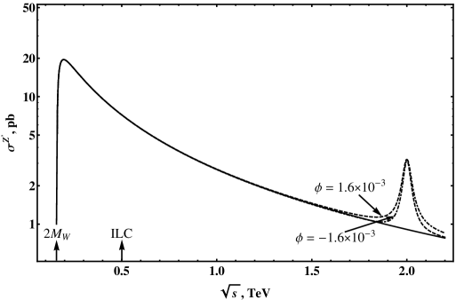
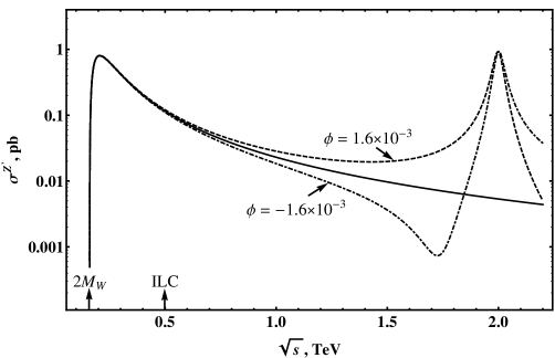
Figure 3: Top panel: Unpolarized total cross section for the process $e^{+}e^{-}\rightarrow W^{+}W^{-}$ for $Z^{\prime}_{\chi}$ from $E_{6}$. Bottom panel: Polarized total cross section. Solid lines correspond to the SM case. Dashed (dash-dotted) lines correspond to a $Z^{\prime}$ model with $\phi=1.6\cdot 10^{-3}$ ($\phi=-1.6\cdot 10^{-3}$), $\Gamma_{2}=0.025\times M_{2}$ and $M_{2}=2~{}\text{TeV}$.

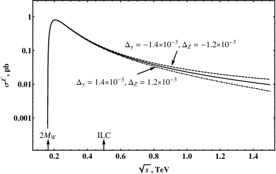
Figure 4: Top panel: Polarized total cross section for the process $e^{+}e^{-}\rightarrow W^{+}W^{-}$ as a function of $\sqrt{s}$ with perfectly polarized electrons ($P_{L}=1$) and unpolarized final states. Solid line corresponds to the SM. Contribution to the cross section caused by $Z^{\prime}$ is determined by different sets of parameters $(\Delta_{\gamma},\Delta_{Z})=(1.4\cdot 10^{-3},1.2\cdot 10^{-3})$ and $(-1.4\cdot 10^{-3},-1.2\cdot 10^{-3})$. Bottom panel: Relative deviation of the polarized total cross section from the SM prediction, $\Delta\sigma/\sigma=(\sigma^{Z^{\prime}}-\sigma^{SM})/\sigma^{SM}$.

The effects of the $Z^{\prime}$ boson shown in Fig. 3 were parametrized by the mass $M_{Z^{\prime}}$ and the $Z$-$Z^{\prime}$ mixing angle $\phi$ while those behaviors and their relative deviations shown in Fig. 4, are parametrized by the effective parameters $(\Delta_{\gamma},\Delta_{Z}$), defined in Eqs. (26) and (27) for the same values of $\phi$ and $M_{Z^{\prime}}$. Rather steep energy behavior of relative deviations of the cross sections can be appreciated from Fig. 4.

As was mentioned in the Introduction, the process (1) is sensitive to a $Z^{\prime}$ in the case of non-zero $Z$-$Z^{\prime}$ mixing. The individual (interference) contributions to the cross section of process (1) rise proportional to $s$. In the SM, the sum over all contributions to the total cross section results in its proper energy dependence that scales like $\log{s}/s$ in the limit when $2M_{W}\ll\sqrt{s}\ll M_{2}$ due to a delicate gauge cancellation. In the case of a non-zero $Z$-$Z^{\prime}$ mixing, the couplings of the $Z_{1}$ differ from those of the SM predictions for $Z$. Then, the gauge cancellation occurring in the SM is destroyed, leading to an enhancement of new physics effects at high energies, though well below $M_{2}$. Unitarity is restored only at energies $\sqrt{s}\gg M_{2}$ independently of details of the extended gauge group.

V Discovery reach on $Z^{\prime}$ parameters

The sensitivity of the polarized differential cross sections to $\Delta_{\gamma}$ and $\Delta_{Z}$ is assessed numerically by dividing the angular range $|\cos\theta|\leq 0.98$ into 10 equal bins, and defining a $\chi^{2}$ function in terms of the expected number of events $N(i)$ in each bin for a given combination of beam polarizations:

$$\chi^{2}=\chi^{2}(\sqrt{s},\Delta_{\gamma},\Delta_{Z})=\sum_{\{P_{L},\,\bar{P}_{L}\}}\sum^{\text{bins}}_{i}\left[\frac{N_{\text{SM}+Z^{\prime}}(i)-N_{\text{SM}}(i)}{\delta N_{\text{SM}}(i)}\right]^{2},$$ (32)

where $N(i)={\cal L}_{\rm int}\,\sigma_{i}\,\varepsilon_{W}$ with ${\cal L}_{\rm int}$ the time-integrated luminosity. Furthermore,

$$\sigma_{i}=\sigma(z_{i},z_{i+1})=\int\limits_{z_{i}}^{z_{i+1}}\left(\frac{d\sigma}{dz}\right)dz,$$ (33)

where $z=\cos\theta$ and polarization indices have been suppressed. Also, $\varepsilon_{W}$ is the efficiency for $W^{+}W^{-}$ reconstruction, for which we take the channel of lepton pairs ($e\nu+\mu\nu$) plus two hadronic jets, giving $\varepsilon_{W}\simeq 0.3$ basically from the relevant branching ratios. The procedure outlined above is followed to evaluate both $N_{\text{SM}}(i)$ and $N_{\text{SM}+Z^{\prime}}(i)$.

The uncertainty on the number of events $\delta N_{\text{SM}}(i)$ combines both statistical and systematic errors where the statistical component is determined by $\delta N^{\text{stat}}_{\text{SM}}(i)=\sqrt{N_{\text{SM}}(i)}$. Concerning systematic uncertainties, an important source is represented by the uncertainty on beam polarizations, for which we assume $\delta P_{L}/P_{L}=\delta{\bar{P}_{L}}/{\bar{P}_{L}}=0.5\%$ with the “standard” envisaged values $|P_{L}|=0.8$ and $|\bar{P}_{L}|=0.5$ :2007sg ; Djouadi:2007ik ; MoortgatPick:2005cw . As for the time-integrated luminosity, for simplicity we assume it to be equally distributed between the different polarization configurations. Another source of systematic uncertainty originates from the efficiency of reconstruction of $W^{\pm}$ pairs which we assume to be $\delta\varepsilon_{W}/\varepsilon_{W}=0.5\%$. Also, in our numerical analysis to evaluate the sensitivity of the differential distribution to model parameters we include initial-state QED corrections to on-shell $W^{\pm}$ pair production in the flux function approach Beenakker:1991jk ; Beenakker:1990sf that assures a good approximation within the expected accuracy of the data.

Figure 5: Discovery reach (see Eq. (34)) at 95% CL on the $Z^{\prime}$ parameters $\Delta_{\gamma},\Delta_{Z}$ obtained from polarized differential cross sections at different sets of polarization: $P_{L}=\pm 0.8,\;\bar{P}_{L}=\mp 0.5$ (solid line), $P_{L}=\pm 0.8,\;\bar{P}_{L}=0$ (short-dashed line), unpolarized beams $P_{L}=0,\;\bar{P}_{L}=0$ (long-dashed line), $\sqrt{s}=0.5~{}\text{TeV}$ and ${\cal L}_{\rm int}=500~{}\text{fb}^{-1}$.

As a criterion to derive the constraints on the coupling constants in the case where no deviations from the SM were observed within the foreseeable uncertainties on the measurable cross sections, we impose that

$$\chi^{2}\leq\chi^{2}_{\mathrm{min}}+\chi^{2}_{\text{CL}},$$ (34)

where $\chi^{2}_{\text{CL}}$ is a number that specifies the chosen confidence level, $\chi^{2}_{\mathrm{min}}$ is the minimal value of the $\chi^{2}$ function. With two independent parameters in Eqs. (17) and (18), the $95\%$ CL is obtained by choosing $\chi^{2}_{\text{CL}}=5.99$.

Figure 6: Discovery reach on the $Z^{\prime}$ parameters $\Delta_{\gamma},\Delta_{Z}$ from the cross section with polarized beams $P_{L}=\pm 0.8,\;\bar{P}_{L}=\mp 0.5$ and different sets of $W^{\pm}$ polarizations. Here, $\sqrt{s}=0.5~{}\text{TeV}$ and ${\cal L}_{\rm int}=500~{}\text{fb}^{-1}$.

From the numerical procedure outlined above, we obtain the allowed regions in $\Delta_{\gamma}$ and $\Delta_{Z}$ determined from the differential polarized cross sections with different sets of polarization (as well as from the unpolarized process (1)) depicted in Fig. 5, where ${\cal L}_{\rm int}=500~{}\text{fb}^{-1}$ has been taken :2007sg ; Djouadi:2007ik ; MoortgatPick:2005cw . According to the condition (34), the values of $\Delta_{\gamma}$ and $\Delta_{Z}$ for which $Z^{\prime}$s can be discovered at the ILC is represented by the region external to the ellipse. The same is true for the AGC model except that, having assumed no renormalization of the residue of the photon pole exchange ($\delta_{\gamma}=0$), in this case $\Delta_{\gamma}$ will be proportional to $s$ times the coefficients $x_{\gamma}$ or $y_{\gamma}$ of Eq. (28), and $\Delta_{Z}$ to a combination of the coefficients $\delta_{Z}$, $x_{Z}$ and $y_{Z}$ (see Table 5). The role of initial beam polarization is seen to be essential in order to set meaningful finite bounds on the parameters.

Figure 7: Discovery reach (95% C.L.) on $Z^{\prime}$ parameters ($\Delta_{\gamma}$, $\Delta_{Z}$) obtained from differential polarized cross sections with ($P_{L}=\pm 0.8,\;\bar{P}_{L}=\mp 0.5$). Dashed straight lines correspond to specific extended gauge models ($\chi$, $\psi$, $\eta$, $I$ and LRS) according to Eq. (35). The segments of the ellipse correspond to the whole classes of $E_{6}$ and LR-models, respectively. Here, $\sqrt{s}=0.5~{}\text{TeV}$ and ${\cal L}_{\rm int}=500~{}\text{fb}^{-1}$.

Analogous to Fig. 5, the discovery reach on the parameters $\Delta_{\gamma},\Delta_{Z}$ from the cross section with polarized beams $P_{L}=\pm 0.8,\;\bar{P}_{L}=\mp 0.5$ and different sets of $W^{\pm}$ polarizations is depicted in Fig. 6 which demonstrates that ${d\sigma(W^{+}_{L}W^{-}_{L})}/{dz}$ is most sensitive to the parameters $\Delta_{\gamma},\Delta_{Z}$ while ${d\sigma(W^{+}_{T}W^{-}_{T})}/{dz}$ has the lowest sensitivity to those parameters. The reason for the lower sensitivity in the $TT$ case is that for $s\gg M_{Z}^{2}$, the NP contributions to these amplitudes only interfere with a sub-dominant part of the SM amplitude Bilenky:1993ms .

As regards the NP scenarios of interest here, one may remark that constraints on $\Delta_{\gamma}$ and $\Delta_{Z}$ of Eqs. (17) and (18) (for the example of $Z^{\prime}$s), are model-independent in the sense that they constrain the whole class of $Z^{\prime}$ models considered. They may turn into constraints on the parameters of specific $Z^{\prime}$ models by replacing expressions (19) and (20). Specializing to those models, one can notice the important linear relation characterizing the deviations from the SM:

$$\Delta_{Z}=\Delta_{\gamma}\cdot\hskip 1.0pt\frac{1}{v\hskip 1.0pt\chi}\hskip 1.0pt\frac{(a^{\prime}/a)}{(a^{\prime}/a)-(v^{\prime}/v)},$$ (35)

where $v$ and $a$ refer to vector and axial-vector couplings. This relation is rather unique, and depends neither on $\phi$ nor on $M_{2}$, only on ratios of the electron couplings with the $Z$ and $Z^{\prime}$ bosons.

In Fig. 7 we depict, as an illustration, the cases corresponding to the models denoted $\chi$, $\psi$, $\eta$ and $I$ originated from $E_{6}$ as well as the LR symmetric model (LRS). The model independent bound on $\Delta_{\gamma}$ and $\Delta_{Z}$ can be converted into limits on the $Z$-$Z^{\prime}$ mixing angle $\phi$ and mass $M_{2}$ for any specific $Z^{\prime}$ model. These model dependent constraints will be presented in the next section along with identification reaches. For fixed $\phi$ and $M_{2}$, every model is represented by a point in the ($\Delta_{\gamma}$, $\Delta_{Z}$) parameter plane. The discovery regions in the $\Delta_{\gamma}$–$\Delta_{Z}$ plot at the ILC are represented by the straight segments lying outside the ellipse. If one varies the mixing angle $\phi$, the point representative of the specific $Z^{\prime}$ model moves along the corresponding line. The intercept of the lines with the elliptic contour, once translated to $\phi$ and $M_{2}$, determine the constraint on these two parameters relevant to $Z$-$Z^{\prime}$ mixing for the individual models.

Also, one can determine the region in the ($\Delta_{\gamma},\Delta_{Z}$) plane relevant to constraining the full class of $E_{6}$ (and LR) $Z^{\prime}$ models obtained by varying the parameters $\cos{\beta}$ and $\alpha_{\text{LR}}$ of Eqs. (2) and (3) within their full allowed ranges. The corresponding discovery region at the ILC for that class of models is the one delimited by the arcs of ellipse indicated in Fig. 7.

VI Identification of $Z^{\prime}$ vs AGC

VI.1 Model independent analysis

We will here discuss how one can differentiate various $Z^{\prime}$ models from similar effects caused by anomalous gauge couplings, following the procedure employed in Refs. Pankov:2005kd ; Osland:2009dp . The philosophy is as follows: A particular $Z^{\prime}$ model will be considered identified, if the measured values of $\Delta_{\gamma}$ and $\Delta_{Z}$ are statistically different from values corresponding to other $Z^{\prime}$ models (for a discussion, see Ref. Osland:2009dp ), and also different from ranges of $(\Delta_{\gamma},\Delta_{Z})$ that can be populated by AGC models. Clearly, at least one of these parameters must exceed some minimal value.

Let us assume the data to be consistent with one of the $Z^{\prime}$ models and call it the “true” model. It has some non-zero values of the parameters $\Delta_{\gamma},\Delta_{Z}$. We want to assess the level at which this “true” model is distinguishable from the AGC models, that can compete with it as sources of the assumed deviations of the cross section from the SM and we call them “tested” models, for any values of the corresponding AGC parameters. We assume for simplicity that all AGC parameters are zero, except the one whose values are probed.

We start by considering as a “tested” AGC model that with a value of $x_{\gamma}$ to be scanned over. To that purpose, we can define a “distance” between the chosen “true” model and the “tested” AGC model(s) by means of a ${\chi}^{2}$ function analogous to Eq. (32) as

$$\chi^{2}=\sum_{\{P_{L},\,\bar{P}_{L}\}}\sum^{\text{bins}}_{i}\left[\frac{N_{Z^{\prime}}(i)-N_{\text{AGC}}(i)}{\delta N_{Z^{\prime}}(i)}\right]^{2},$$ (36)

with $\delta N_{Z^{\prime}}(i)$ defined in the same way as $\delta N_{\text{SM}}(i)$ but, in this case, the statistical uncertainty refers to the $Z^{\prime}$ model and therefore depends on the relevant, particular, values of $\Delta_{\gamma}$ and $\Delta_{Z}$.

On the basis of such $\chi^{2}$ we can study whether these “tested” models can be excluded or not to a given confidence level (which we assume to be 95%), once the considered $Z^{\prime}$ model (defined in terms of $\Delta_{\gamma}$, $\Delta_{Z}$) has been assumed as “true”. In our explicit example, we want to determine the range in $x_{\gamma}$ for which there is “confusion” of deviations from the SM cross sections between the selected “true” $Z^{\prime}$ model and the AGC one, by imposing the condition, similar to Eq. (34). Then we scan all values of $\Delta_{\gamma}$, $\Delta_{Z}$ allowed by the $Z^{\prime}$ models down to their discovery reach, and determine by iteration in this procedure the general confusion region between the class of $Z^{\prime}$ models considered here and the AGC model with $x_{\gamma}\neq 0$.

Besides the dependence on the c.m. energy $\sqrt{s}$, the $\chi^{2}$ function defined above can be considered a function of three independent variables, $\Delta_{\gamma}$ and $\Delta_{Z}$ from the $Z^{\prime}$ model, and, in our starting example, the parameter $x_{\gamma}$ of the AGC scenario. The contours of the confusion regions, at given $\sqrt{s}$, are thus defined by the region inside of which (in the $\Delta_{\gamma}$-$\Delta_{Z}$ space)

$$\chi^{2}(\Delta_{\gamma},\Delta_{Z},x_{\gamma})=\chi^{2}_{\mathrm{min}}+\chi^{2}_{\text{CL}},$$ (37)

for any value of $x_{\gamma}$ compatible with experimental limits.

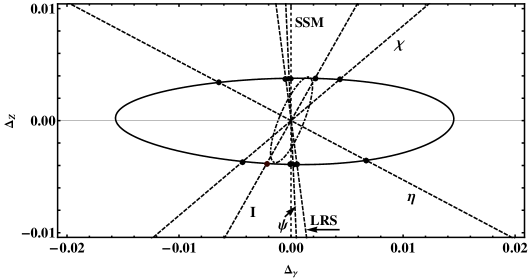
Figure 8: The outer ellipse (solid) shows the confusion region (95% C.L., see Eq. (37)) in the parameter plane ($\Delta_{\gamma},\Delta_{Z}$), outside of which a generic $Z^{\prime}$ model can be identified against an AGC model with non-vanishing parameter $x_{\gamma}$. Polarized cross section with $P_{L}=\pm 0.8$ and $\bar{P}_{L}=\mp 0.5$ are assumed. The dashed inner ellipse reproduces the discovery reach on the $Z^{\prime}$ of Fig. 7, corresponding to $x_{\gamma}=0$ in Eq. (37), where the AGC model coincides with the SM. The dashed straight lines correspond to specific extended gauge models ($\chi$, $\psi$, $\eta$, I and LRS). Here, $\sqrt{s}=0.5~{}\text{TeV}$ and ${\cal L}_{\rm int}=500~{}\text{fb}^{-1}$.

In Fig. 8 we show the region of confusion in the $Z^{\prime}$ parameter plane ($\Delta_{\gamma},\Delta_{Z}$), outside of which the $Z^{\prime}$ model can be identified at the 95% C.L. against the AGC model for any value of the parameter $x_{\gamma}$. It is obtained from the polarized cross section with $P_{L}=\pm 0.8$ and $\bar{P}_{L}=\mp 0.5$ using the algorithm outlined above. Also, note that the inner dash-dotted ellipse in Fig. 8 delimits the discovery reach on $Z^{\prime}$ parameters.

The graphical representation of the region of confusion presented in Fig. 8 is straightforward. Equation (37) defines a three-dimensional surface enclosing a volume in the ($\Delta_{\gamma},\Delta_{Z},x_{\gamma}$) parameter space in which there can be discovery as well as confusion between $Z^{\prime}$ and (in this case) the $x_{\gamma}$-AGC model. The planar surface delimited by the solid ellipse is determined by the projection of such three-dimensional surface, hence of the corresponding confusion region, onto the plane ($\Delta_{\gamma},\Delta_{Z}$). Any determination of $\Delta_{\gamma}$ and $\Delta_{Z}$ in the planar domain exterior to the ellipse would allow both $Z^{\prime}$ discovery and identification against the $x_{\gamma}$-AGC model. Similar to the case of discovery, also in the case of $Z^{\prime}$ identification the bounds on $\Delta_{\gamma}$ and $\Delta_{Z}$ could be translated into limits on the $Z$-$Z^{\prime}$ mixing angle $\phi$ and mass $M_{2}$ for any specific $Z^{\prime}$ model.

The procedure outlined above can be repeated for all other types of models with AGC parameters ($\delta_{Z}$, $x_{Z}$, $y_{\gamma}$, $y_{Z}$), and consequently one can evaluate the corresponding “confusion regions” in the ($\Delta_{\gamma},\Delta_{Z}$) parameter plane. The results of this kind of analysis are represented in Fig. 9 displaying the overlap of the confusion regions (95% C.L.) in the parameter plane ($\Delta_{\gamma},\Delta_{Z}$) for a generic $Z^{\prime}$ vector model and AGC models with parameters varying one at a time.

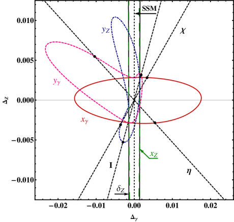
Figure 9: The closed contours indicate regions of $(\Delta_{\gamma},\Delta_{Z})$ that can be populated by variations of an AGC parameter, such as for example $x_{\gamma}$. They are thus confusion regions (95%C.L.) in the parameter plane ($\Delta_{\gamma},\Delta_{Z}$) for a generic $Z^{\prime}$ model and AGC models with parameters taking non-vanishing values, one at a time: $x_{\gamma}$, $x_{Z}$, $y_{\gamma}$, $y_{Z}$ and $\delta_{Z}$. Polarized cross sections with $P_{L}=\pm 0.8$ and $\bar{P}_{L}=\mp 0.5$ have been exploited. Dashed straight lines correspond to specific $Z^{\prime}$ models ($\chi$, $\psi$, $\eta$, I and LRS). Here, $\sqrt{s}=0.5~{}\text{TeV}$ and ${\cal L}_{\rm int}=500~{}\text{fb}^{-1}$.

The resulting confusion area (obtained from the overlap of all confusion regions) turns out to be open in the vertical direction, i.e., along the $\Delta_{Z}$ axis. The reason is that the $Z^{\prime}$ model defined by a particular parameter set where ($\Delta_{\gamma}=0,\Delta_{Z}$) is indistinguishable from those originating from AGC with the same $\delta_{Z}=\Delta_{Z}$. Moreover, from a comparison of the confusion region depicted in Fig. 9 with the corresponding discovery reach presented in Fig. 7 one can conclude that all $Z^{\prime}$ models might be discovered in the process (1) with polarized beams. However, they may not all be identified, the reason being that the confusion region shown in Fig. 9 is not closed, in contrast to the reach shown in Fig. 7.

An example relevant to the current discussion can be found in the SSM model. In fact, from Eq. (35) one can conclude that the signature space of the SSM model in the ($\Delta_{\gamma},\Delta_{Z}$) parameter plane extends along $\Delta_{Z}$. It implies that the SSM might be discovered in the process (1) but not separated from AGC models characterized by the parameter $\Delta_{Z}$. More generally, those models where the $Z^{\prime}$-electron couplings satisfy the equation $v^{\prime}/a^{\prime}=v/a$ that, as follows from Eq. (26), lead to $\Delta_{\gamma}=0$ can not be distinguished from the AGC case in the $W^{\pm}$ pair production process. However, all other $Z^{\prime}$ models (apart from the considered exceptional case) described by the pair of parameters ($\Delta_{\gamma},\Delta_{Z}$) that are located outside of the confusion area shown in Fig. 9 can be identified. Notice that the above constraint on the electron couplings is fulfilled for an $E_{6}$ model at $\beta=87^{\circ}$ and for an LRS model with $\alpha_{LR}=1.36$.

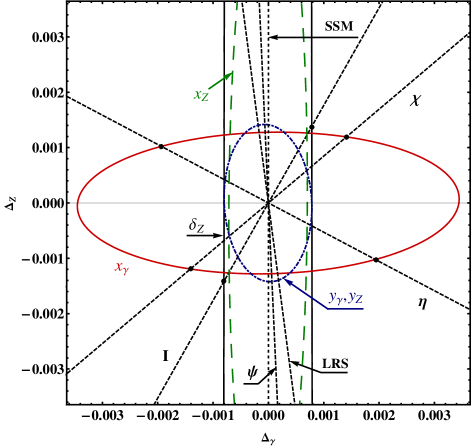
Figure 10: Same as in Fig. 9 but obtained from combined analysis of the process (1) with polarized initial beams and polarized $W^{\pm}$ final states. The $x_{Z}$ contour closes at $\Delta_{Z}\simeq\pm 0.006$.

The results of a further potential extension of the present analysis are presented in Fig. 10 where the feasibility of measuring polarized $W^{\pm}$ states in the process (1) is assumed. This assumption is based on the experience gained at LEP2 on measurements of $W$ polarisation LEP2Wpolar . The relevant theoretical framework for measurement of $W^{\pm}$ polarisation was described in gounaris ; Gounaris:1992kp . The method exploited for the measurement of $W$ polarisation is based on the spin density matrix elements that allow to obtain the differential cross sections for polarised $W$ bosons. Information on spin density matrix elements as functions of the $W^{-}$ production angle with respect to the electron beam direction was extracted from the decay angles of the charged lepton in the $W^{-}$ ($W^{+}$) rest frame.

VI.2 Model dependent analysis

As mentioned above, the ranges of $\Delta_{\gamma}$ and $\Delta_{Z}$ allowed to the specific models in Figs. 9 and 10 can be translated into discovery and identification reaches on the mixing angle $\phi$ and the heavier gauge boson mass $M_{2}$, using Eqs. (26)–(27). The resulting allowed regions, discovery and identification (at the 95% CL) in the ($\phi,M_{2}$) plane is limited in this case by the thick dashed and solid lines, respectively, in Figs. 11– 12 for some specific $E_{6}$ models. These limits are obtained from the polarized differential distributions of $W$ with collider energy $\sqrt{s}=0.5~{}\text{TeV}$ and integrated luminosity ${\cal L}_{\rm int}=500~{}\text{fb}^{-1}$. Also, an indicative typical lower bound on $M_{2}$ from direct searches at the LHC with $\sqrt{s}=7~{}\text{TeV}$ Chatrchyan:2012it ; atlas-dilepton is reported in these figures as horizontal straight lines. The vertical arrows then indicate the range of available $Z^{\prime}$ mass values according to LHC limits.

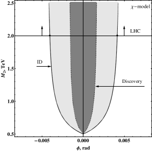
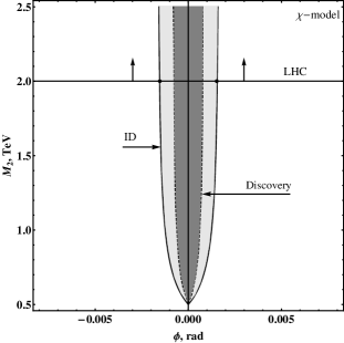
Figure 11: Left: Discovery (dashed line) and identification (solid line) reach for the $\chi$ model in the $\left(\phi,M_{2}\right)$ plane obtained from polarized initial $e^{+}$ and $e^{-}$ beams with ($P_{L}=\pm 0.8,\;\bar{P}_{L}=\mp 0.5$) and unpolarized final $W^{\pm}$ states. Right: The same with polarized final $W^{\pm}$ states. Here, $\sqrt{s}=0.5~{}\text{TeV}$ and ${\cal L}_{\rm int}=500~{}\text{fb}^{-1}$. The horizontal line with vertical arrows, here and in the next figures, approximately indicates the range of $M_{2}$ currently allowed by LHC.

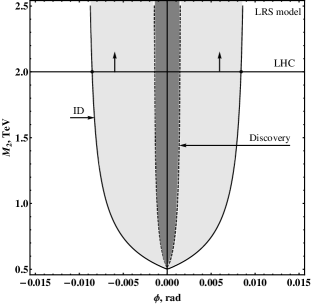
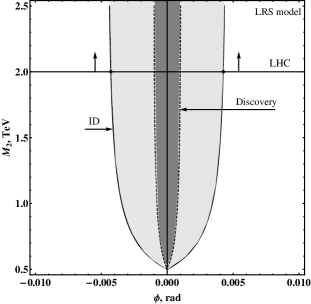
Figure 12: Same as in Fig.11 but for the LRS model.

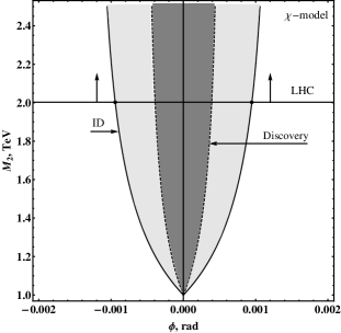
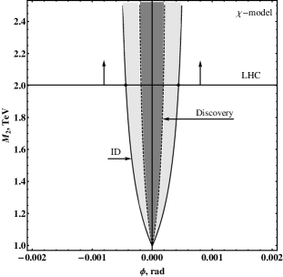
Figure 13: Left: Discovery (dashed line) and identification (solid line) reach for the $\chi$ model in the $\left(\phi,M_{2}\right)$ plane obtained from polarized initial $e^{+}$ and $e^{-}$ beams with ($P_{L}=\pm 0.8,\;\bar{P}_{L}=\mp 0.5$) and unpolarized final $W^{\pm}$ states. Right: The same with polarized final $W^{\pm}$ states. Here, $\sqrt{s}=1~{}\text{TeV}$ and ${\cal L}_{\rm int}=1~{}\text{ab}^{-1}$.

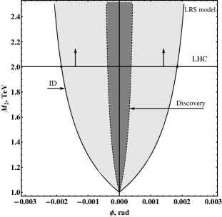
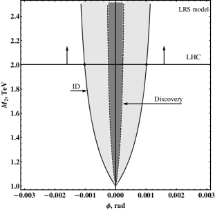
Figure 14: Same as in Fig.13 but for the LRS model.

Table 1: Discovery and identification reach on the $Z$-$Z^{\prime}$ mixing angle $\phi$ for $Z^{\prime}$ models with $M_{2}=2~{}\text{TeV}$ obtained from the polarized differential cross section with ($P_{L}=\pm 0.8,\;\bar{P}_{L}=\mp 0.5$) and unpolarized final states for the case $\sqrt{s}=0.5~{}\text{TeV}$ and ${\cal L}_{\rm int}=500~{}\text{fb}^{-1}$. The corresponding limits for polarized $W$s are given in parenthesis.

$Z^{\prime}$ model	$\chi$	$\psi$	$\eta$	I	LRS	SSM
$\phi^{\text{DIS}},10^{-3}$	$\pm 1.5(0.8)$	$\pm 2.3(1.4)$	$\pm 1.6(1.3)$	$\pm 2.0(0.8)$	$\pm 1.4(1.0)$	$\pm 1.2(0.7)$
$\phi^{\text{ID}},10^{-3}$	$\pm 3.8(1.5)$	$\pm 36.8(18.5)$	$\pm 17.4(3.2)$	$\pm 4.3(1.2)$	$\pm 8.1(4.2)$	–

Figures 11 and 12 show that the process $e^{+}e^{-}\rightarrow W^{+}W^{-}$ at $0.5~{}\text{TeV}$ has a potential sensitivity to the mixing angle $\phi$ of the order of $10^{-4}$–$10^{-3}$ or even less, depending on the mass $M_{2}$. This sensitivity would increse for the c.m. energy $\sqrt{s}$ approaching $M_{2}$ because the contribution of the $Z_{2}$ exchange diagram in Fig. 1 would be enhanced. However, $Z^{\prime}$ bosons relevant to the extended models under study with mass below $\sim 2.0-2.3~{}\text{TeV}$ are already excluded by LHC data, and the ILC c.m. energies considered here are therefore quite far from the admissible $M_{2}$. Conversely, for masses $M_{2}$ much larger than $\sqrt{s}$ such that the $Z_{2}$ exchange contribution $|\chi_{2}/\chi|$ is much less than unity, the limiting contour is mostly determined by the modification (10) of the $Z$ couplings to electrons. The discovery and identification reaches on $\phi$ at $M_{2}=2~{}\text{TeV}$ are summarized in Table 1.

For the ILC with higher energy and luminosity, $\sqrt{s}=1~{}\text{TeV}$ and ${\cal L}_{\rm int}=1$ ab^-1, one expects further improvement of the discovery and identification reach on the $Z$-$Z^{\prime}$ mixing angle and $M_{2}$ (see Figures 13, 14 and Table 2).

Table 2: Same as in Table 1 but for ILC with $\sqrt{s}=1~{}\text{TeV}$ and ${\cal L}_{\rm int}=1~{}\text{ab}^{-1}$.

$Z^{\prime}$ model	$\chi$	$\psi$	$\eta$	I	LRS	SSM
$\phi^{\text{DIS}},10^{-4}$	$\pm 3.8(1.8)$	$\pm 5.8(3.4)$	$\pm 4.6(3.2)$	$\pm 4.4(1.9)$	$\pm 3.7(2.4)$	$\pm 3.1(1.7)$
$\phi^{\text{ID}},10^{-4}$	$\pm 9.0(4.2)$	$\pm 94(45)$	$\pm 24(9.5)$	$\pm 6.1(2.8)$	$\pm 18(10)$	–

As already mentioned, the horizontal lines in Figs. 11–14 denote the current LHC lower limits on $M_{2}$, therefore only the upper parts, as indicated by the vertical arrows, will be available for discovery and identification of a $Z^{\prime}$ via indirect manifestations at the ILC with the considered values for the c.m. energy of 0.5 and 1 TeV. Since those limits are so much higher than $\sqrt{s}$, the corrections from finite $Z^{\prime}$ widths, assumed in the range $\Gamma_{Z^{\prime}}=(0.01-0.10)M_{Z^{\prime}}$ Langacker:2008yv , are found to be numerically negligible in the “working” regions indicated in those figures by the horizontal lines and vertical arrows. Tables 1 and 2 demonstrate that ILC (0.5 TeV) and ILC (1 TeV) allow to improve current bounds on $Z$–$Z^{\prime}$ mixing for most of the $Z^{\prime}$ models, and also differentiating $Z^{\prime}$ from AGC is feasible.

VI.3 Low-energy option

Currently, physics at the ILC in a low-energy option is extensively studied and discussed, as it in this mode might act as a “Higgs factory”. The results for discovery and identification reach on $Z$-$Z^{\prime}$ mixing and mass $M_{2}$ obtained from the ILC with $\sqrt{s}=0.25$ TeV and 0.35 TeV are summarized in Tables 3 and 4.

Table 3: Same as in Table 1 but for the ILC with $\sqrt{s}=0.25~{}\text{TeV and}$ ${\cal L}_{\rm int}=100$ fb^-1.

$Z^{\prime}$ model	$\chi$	$\psi$	$\eta$	I	LRS	SSM
$\phi^{\text{DIS}},10^{-3}$	$\pm 5.1(3.8)$	$\pm 8.4(7.0)$	$\pm 6.8(6.7)$	$\pm 5.7(3.9)$	$\pm 5.4(4.9)$	$\pm 4.4(3.6)$
$\phi^{\text{ID}},10^{-3}$	$\pm 14(6.8)$	$\pm 109(86)$	$\pm 29(14)$	$\pm 7.8(5.9)$	$\pm 45(21)$	–

Table 4: Same as in Table 3 but for the ILC with $\sqrt{s}=0.35~{}\text{TeV}$, and two values of integrated luminosity.

$Z^{\prime}$ model		$\chi$	$\psi$	$\eta$	I	LRS	SSM
$100~{}\text{fb}^{-1}$	$\phi^{\text{DIS}},10^{-3}$	$\pm 3.7(2.4)$	$\pm 6.0(4.5)$	$\pm 4.9(4.3)$	$\pm 4.1(2.5)$	$\pm 3.9(3.1)$	$\pm 3.2(2.3)$
	$\phi^{\text{ID}},10^{-3}$	$\pm 8.4(4.6)$	$\pm 77(61)$	$\pm 27(9.4)$	$\pm 13.5(3.8)$	$\pm 19(14)$	–
$500~{}\text{fb}^{-1}$	$\phi^{\text{DIS}},10^{-3}$	$\pm 2.3(1.3)$	$\pm 3.4(2.3)$	$\pm 2.5(2.1)$	$\pm 3.1(1.4)$	$\pm 2.1(1.6)$	$\pm 1.8(1.2)$
	$\phi^{\text{ID}},10^{-3}$	$\pm 5.9(2.4)$	$\pm 54(30)$	$\pm 15(4.7)$	$\pm 4.0(1.9)$	$\pm 16(6.8)$	–

The comparison of these constraints with those obtained from electroweak precision data derived mostly from on-$Z$-resonance experiments at LEP1 and SLC Erler:2009jh shows that the ILC (0.25 TeV) and ILC (0.35 TeV) allow to obtain bounds on $Z$-$Z^{\prime}$ mixing at the same level as those of current experimental limits, thereby providing complementary bounds on $Z^{\prime}$s.

Increasing the luminosity at fixed energy, asymptotically allows for an increase of the sensitivity $\propto 1/\sqrt{{\cal L}_{\rm int}}$. In the example shown in Table 4, this behavior is not quite reached, due to the impact of systematic uncertainties.

VII Concluding remarks

We have discussed the foreseeable sensitivity to $Z^{\prime}$s in $W^{\pm}$-pair production cross sections at the ILC, especially as regards the potential of distinguishing observable effects of a $Z^{\prime}$ from analogous ones due to competitor models with Anomalous Gauge Couplings that can lead to the same or similar new physics experimental signatures. The discovery and identification reaches on $E_{6}$ and LRS models have been determined in the parameter plane spanned by the $Z$-$Z^{\prime}$ mixing angle $\phi$, and $Z^{\prime}$ mass, $M_{2}$.

We have shown that the sensitivity of the ILC for probing the $Z$-$Z^{\prime}$ mixing and its capability to distinguish these two new physics scenarios is substantially enhanced when the polarization of the initial beams (and also, possibly, the produced $W^{\pm}$ bosons) are considered.

Appendix A. Helicity amplitudes

In this appendix, we collect the helicity amplitudes for the different initial ($e^{+}e^{-}$) and final-state ($W^{+}W^{-}$) polarizations. In Table 5 we quote the amplitudes for the case of Anomalous Gauge Couplings gounaris ; Gounaris:1992kp , whereas in Table 6 we give the corresponding results for the case of a $Z^{\prime}$.

Table 5: Helicity amplitudes for $e^{+}e^{-}\rightarrow W^{+}W^{-}$ in the presence of AGC gounaris ; Gounaris:1992kp . To obtain the amplitude $F_{\lambda\tau\tau^{\prime}}(s,\cos\theta)$ for definite helicity $\lambda=\pm 1/2$ and definite spin orientations $\tau(W^{-})$ and $\tau^{\prime}(W^{+})$ of the $W^{\pm}$, the elements in the corresponding column have to be multiplied by the common factor on top of the column. Subsequently, the elements in a specific column have to be multiplied by the corresponding elements in the first column and the sum over all elements is to be taken. In the last column, the amplitude for the case of $\tau=\pm 1$, $\tau^{\prime}=0$ is obtained by replacing $\tau^{\prime}$ by $-\tau$ in the elements of this last column.

$e^{+}_{-\lambda}e^{-}_{\lambda}\rightarrow W^{+}_{L}W^{-}_{L}$	$\tau=\tau^{\prime}=0$
	$-\frac{e^{2}s\lambda}{2}\sin\theta$
$\frac{2\lambda-1}{4\hskip 2.0ptt\hskip 2.0pts^{2}_{W}}$	$\frac{s}{2M_{W}^{2}}[\cos\theta-\beta_{W}(1+\frac{2M_{W}^{2}}{s})]$
$-\frac{2}{s}+\frac{2(\cot\theta_{W}+\delta_{Z})}{s-M_{Z}^{2}}(v-2a\lambda)$	$-\beta_{W}(1+\frac{s}{2M^{2}_{W}})$
$-\frac{x_{\gamma}}{s}+\frac{x_{Z}}{s-M_{Z}^{2}}(v-2a\lambda)$	$-\beta_{W}\frac{s}{M^{2}_{W}}$
$e^{+}_{-\lambda}e^{-}_{\lambda}\rightarrow W^{+}_{T}W^{-}_{T}$	$\tau=\tau^{\prime}=\pm 1$	$\tau=-\tau^{\prime}=\pm 1$
	$-\frac{e^{2}s\lambda}{2}\sin\theta$	$-\frac{e^{2}s\lambda}{2}\sin\theta$
$\frac{2\lambda-1}{4\hskip 2.0ptt\hskip 2.0pts^{2}_{W}}$	$\cos\theta-\beta_{W}$	$-\cos\theta-2\tau\lambda$
$-\frac{2}{s}+\frac{2(\cot\theta_{W}+\delta_{Z})}{s-M_{Z}^{2}}(v-2a\lambda)$	$-\beta_{W}$	$0$
$-\frac{y_{\gamma}}{s}+\frac{y_{Z}}{s-M_{Z}^{2}}(v-2a\lambda)$	$-\beta_{W}\frac{s}{M^{2}_{W}}$	$0$
$e^{+}_{-\lambda}e^{-}_{\lambda}\rightarrow W^{+}_{T}W^{-}_{L}$	$\tau=0$, $\tau^{\prime}=\pm 1$	$\tau=\pm 1$, $\tau^{\prime}=0$
	$-\frac{e^{2}s\lambda}{2\sqrt{2}}(\tau^{\prime}\cos\theta-2\lambda)$	$\frac{e^{2}s\lambda}{2\sqrt{2}}(\tau\cos\theta+2\lambda)$
$\frac{2\lambda-1}{4\hskip 2.0ptt\hskip 2.0pts^{2}_{W}}$	$\frac{\sqrt{s}}{2M_{W}}[\cos\theta(1+\beta_{W}^{2})-2\beta_{W}]$	$\frac{\sqrt{s}}{2M_{W}}[\cos\theta(1+\beta_{W}^{2})-2\beta_{W}]$
	$-\frac{2M_{W}}{\sqrt{s}}\frac{\tau^{\prime}\sin^{2}\theta}{\tau^{\prime}\cos\theta-2\lambda}$	$-\frac{2M_{W}}{\sqrt{s}}\frac{\tau\sin^{2}\theta}{\tau\cos\theta+2\lambda}$
$-\frac{2}{s}+\frac{2(\cot\theta_{W}+\delta_{Z})}{s-M_{Z}^{2}}(v-2a\lambda)$	$-\beta_{W}\frac{\sqrt{s}}{M_{W}}$	$-\beta_{W}\frac{\sqrt{s}}{M_{W}}$
$-\frac{x_{\gamma}+y_{\gamma}}{s}+\frac{x_{Z}+y_{Z}}{s-M_{Z}^{2}}(v-2a\lambda)$	$-\beta_{W}\frac{\sqrt{s}}{M_{W}}$	$-\beta_{W}\frac{\sqrt{s}}{M_{W}}$

Note that the quantity $\delta_{Z}$ appearing in Table 5 is different from, but plays a role similar to that of $\Delta_{Z}$ entering in the parametrization of $Z^{\prime}$ effects. Furthermore, in analogy with the $\Delta_{\gamma}$ which enters the description of $Z^{\prime}$ effects, one could imagine a factor $(1+\delta_{\gamma})$ multiplying the photon-exchange amplitudes in Table 5. Such a term could be induced by dimension-8 operators, but $\delta_{\gamma}$ would have to vanish as $s\rightarrow 0$, due to gauge invariance.

Table 6: Helicity amplitudes for $e^{+}e^{-}\rightarrow\gamma,Z_{1},Z_{2}\rightarrow W^{+}W^{-}$.

$e^{+}_{-\lambda}e^{-}_{\lambda}\rightarrow W^{+}_{L}W^{-}_{L}$	$\tau=\tau^{\prime}=0$
	$-\frac{e^{2}s\lambda}{2}\sin\theta$
$\frac{2\lambda-1}{4\hskip 2.0ptt\hskip 2.0pts^{2}_{W}}$	$\frac{s}{2M_{W}^{2}}[\cos\theta-\beta_{W}(1+\frac{2M_{W}^{2}}{s})]$
$-\frac{2}{s}+\frac{2\,g_{WWZ_{1}}}{s-M_{1}^{2}+iM_{1}\Gamma_{1}}\,(v_{1}-2a_{1}\lambda)$	$-\beta_{W}(1+\frac{s}{2M^{2}_{W}})$
$+\frac{2\,g_{WWZ_{2}}}{s-M_{2}^{2}+iM_{2}\Gamma_{2}}\,(v_{2}-2a_{2}\lambda)$
$\approx-\frac{2(1+\Delta_{\gamma})}{s}+\frac{2(\cot\theta_{W}+\Delta_{Z})}{s-M_{Z}^{2}}(v-2a\lambda)$
$e^{+}_{-\lambda}e^{-}_{\lambda}\rightarrow W^{+}_{T}W^{-}_{T}$	$\tau=\tau^{\prime}=\pm 1$	$\tau=-\tau^{\prime}=\pm 1$
	$-\frac{e^{2}s\lambda}{2}\sin\theta$	$-\frac{e^{2}s\lambda}{2}\sin\theta$
$\frac{2\lambda-1}{4\hskip 2.0ptt\hskip 2.0pts^{2}_{W}}$	$\cos\theta-\beta_{W}$	$-\cos\theta-2\tau\lambda$
$-\frac{2}{s}+\frac{2\,g_{WWZ_{1}}}{s-M_{1}^{2}+iM_{1}\Gamma_{1}}\,(v_{1}-2a_{1}\lambda)$	$-\beta_{W}$	$0$
$+\frac{2\,g_{WWZ_{2}}}{s-M_{2}^{2}+iM_{2}\Gamma_{2}}\,(v_{2}-2a_{2}\lambda)$
$\approx-\frac{2(1+\Delta_{\gamma})}{s}+\frac{2(\cot\theta_{W}+\Delta_{Z})}{s-M_{Z}^{2}}(v-2a\lambda)$
$e^{+}_{-\lambda}e^{-}_{\lambda}\rightarrow W^{+}_{T}W^{-}_{L}$	$\tau=0$, $\tau^{\prime}=\pm 1$	$\tau=\pm 1$, $\tau^{\prime}=0$
	$-\frac{e^{2}s\lambda}{2\sqrt{2}}(\tau^{\prime}\cos\theta-2\lambda)$	$\frac{e^{2}s\lambda}{2\sqrt{2}}(\tau\cos\theta+2\lambda)$
$\frac{2\lambda-1}{4\hskip 2.0ptt\hskip 2.0pts^{2}_{W}}$	$\frac{\sqrt{s}}{2M_{W}}[\cos\theta(1+\beta_{W}^{2})-2\beta_{W}]$	$\frac{\sqrt{s}}{2M_{W}}[\cos\theta(1+\beta_{W}^{2})-2\beta_{W}]$
	$-\frac{2M_{W}}{\sqrt{s}}\frac{\tau^{\prime}\sin^{2}\theta}{\tau^{\prime}\cos\theta-2\lambda}$	$-\frac{2M_{W}}{\sqrt{s}}\frac{\tau\sin^{2}\theta}{\tau\cos\theta+2\lambda}$
$-\frac{2}{s}+\frac{2\,g_{WWZ_{1}}}{s-M_{1}^{2}+iM_{1}\Gamma_{1}}\,(v_{1}-2a_{1}\lambda)$	$-\beta_{W}\frac{\sqrt{s}}{M_{W}}$	$-\beta_{W}\frac{\sqrt{s}}{M_{W}}$
$+\frac{2\,g_{WWZ_{2}}}{s-M_{2}^{2}+iM_{2}\Gamma_{2}}\,(v_{2}-2a_{2}\lambda)$
$\approx-\frac{2(1+\Delta_{\gamma})}{s}+\frac{2(\cot\theta_{W}+\Delta_{Z})}{s-M_{Z}^{2}}(v-2a\lambda)$

References

- (1) P. Langacker, Rev. Mod. Phys. 81, 1199-1228 (2009) [arXiv:0801.1345 [hep-ph]].
- (2) T. G. Rizzo, [hep-ph/0610104].
- (3) A. Leike and S. Riemann, Z. Phys. C 75, 341 (1997) [hep-ph/9607306].
- (4) A. Leike, Phys. Rept. 317, 143-250 (1999) [hep-ph/9805494].
- (5) S. Riemann, eConf C 050318, 0303 (2005) [hep-ph/0508136].
- (6) J. L. Hewett, T. G. Rizzo, Phys. Rept. 183, 193 (1989).
- (7) J. Erler, P. Langacker, S. Munir, E. Rojas, JHEP 0908, 017 (2009) [arXiv:0906.2435 [hep-ph]].
- (8) P. Langacker, [arXiv:0911.4294 [hep-ph]].
- (9) S. Chatrchyan et al. [CMS Collaboration], Phys. Lett. B714, 158-179 (2012) [arXiv:1206.1849 [hep-ex]].
- (10) ATLAS Collaboration, Note ATLAS-CONF-2012-007 (March 2012).
- (11) P. Osland, A. A. Pankov, A. V. Tsytrinov, N. Paver, Phys. Rev. D79, 115021 (2009) [arXiv:0904.4857 [hep-ph]].
- (12) J. Brau et al. [ILC Collaboration], “ILC Reference Design Report Volume 1 - Executive Summary,” arXiv:0712.1950 [physics.acc-ph].
- (13) G. Aarons et al. [ILC Collaboration], “International Linear Collider Reference Design Report Volume 2: PHYSICS AT THE ILC,” arXiv:0709.1893 [hep-ph].
- (14) A. A. Pankov, N. Paver, Phys. Lett. B272, 425-430 (1991).
- (15) A. A. Pankov, N. Paver, Phys. Rev. D48, 63-77 (1993).
- (16) A. A. Pankov, N. Paver, Phys. Lett. B324, 224-230 (1994).
- (17) A. A. Pankov, N. Paver, C. Verzegnassi, Int. J. Mod. Phys. A13, 1629-1650 (1998) [hep-ph/9701359].
- (18) D. -W. Jung, K. Y. Lee, H. S. Song, C. Yu, J. Korean Phys. Soc. 36, 258-264 (2000) [hep-ph/9905353].
- (19) B. Ananthanarayan, M. Patra, P. Poulose, JHEP 1102, 043 (2011) [arXiv:1012.3566 [hep-ph]].
- (20) G. Gounaris, J. L. Kneur, J. Layssac, G. Moultaka, F. M. Renard and D. Schildknecht, Proceedings of the Workshop Collisions at 500 GeV: the Physics Potential, Ed. P.M. Zerwas (1992), DESY 92-123B, p.735.
- (21) G. Gounaris, J. Layssac, G. Moultaka, F. M. Renard, Int. J. Mod. Phys. A8, 3285-3320 (1993).
- (22) G. Moortgat-Pick, T. Abe, G. Alexander, B. Ananthanarayan, A. A. Babich, V. Bharadwaj, D. Barber, A. Bartl et al., Phys. Rept. 460, 131-243 (2008) [hep-ph/0507011].
- (23) P. Osland, A. A. Pankov, A. V. Tsytrinov, Eur. Phys. J. C67, 191-204 (2010) [arXiv:0912.2806 [hep-ph]].
- (24) P. Langacker and M. -x. Luo, Phys. Rev. D 45, 278 (1992).
- (25) K. Hagiwara, R. D. Peccei, D. Zeppenfeld and K. Hikasa, Nucl. Phys. B 282, 253 (1987)
- (26) M. S. Bilenky, J. L. Kneur, F. M. Renard and D. Schildknecht, Nucl. Phys. B 409, 22 (1993).
- (27) M. S. Bilenky, J. L. Kneur, F. M. Renard and D. Schildknecht, Nucl. Phys. B 419, 240 (1994) [hep-ph/9312202].
- (28) K. Nakamura et al. [Particle Data Group Collaboration], J. Phys. G 37, 075021 (2010).
- (29) J. Fleischer, K. Kolodziej and F. Jegerlehner, Phys. Rev. D 47, 830 (1993).
- (30) W. Beenakker and A. Denner, Int. J. Mod. Phys. A 9, 4837 (1994).
- (31) A. Denner, S. Dittmaier, M. Roth and L. H. Wieders, Phys. Lett. B 612, 223 (2005) [Erratum-ibid. B 704, 667 (2011)] [hep-ph/0502063].
- (32) A. Denner, S. Dittmaier, M. Roth and L. H. Wieders, Nucl. Phys. B 724, 247 (2005) [Erratum-ibid. B 854, 504 (2012)] [hep-ph/0505042].
- (33) W. Beenakker, F. A. Berends and T. Sack, Nucl. Phys. B 367, 287 (1991).
- (34) W. Beenakker, K. Kolodziej and T. Sack, Phys. Lett. B 258, 469 (1991).
- (35) A. A. Pankov, N. Paver and A. V. Tsytrinov, Phys. Rev. D 73, 115005 (2006) [arXiv:hep-ph/0512131].
-
(36)
G. Abbiendi et al., [OPAL collaboration], Phys.
Lett. B585, 223 (2004);
P. Achard et al., [L3 collaboration], Phys. Lett. B557, 147 (2003);
J. Abdallah et al., [DELPHI Collaboration], Eur. Phys. J. C 54, 345 (2008) [arXiv:0801.1235 [hep-ex]];
J.P. Couchman, A measurement of the triple gauge boson couplings and boson polarisation in -pair production at LEP2, Ph.D. thesis, University College London, 2000.