A dynamical analysis of the Kepler-11 planetary system

Abstract

The Kepler-11 star hosts at least six transiting super-Earth planets detected through the precise photometric observations of the Kepler mission (Lissauer et al.). In this paper, we re-analyze the available Kepler data, using the direct $N$-body approach rather than an indirect TTV method in the discovery paper. The orbital modeling in the realm of the direct approach relies on the whole data set, not only on the mid–transits times. Most of the results in the original paper are confirmed and extended. We constrained the mass of the outermost planet g to less than 30 Earth masses. The mutual inclinations between orbits b and c as well as between orbits d and e are determined with a good precision, in the range of [1,5] degrees. Having several solutions to four qualitative orbital models of the Kepler-11 system, we analyze its global dynamics with the help of dynamical maps. They reveal a sophisticated structure of the phase space, with narrow regions of regular motion. The dynamics are governed by a dense net of three– and four–body mean motion resonances, forming the Arnold web. Overlapping of these resonances is a main source of instability. We found that the Kepler-11 system may be long-term stable only in particular multiple resonant configurations with small relative inclinations. The mass-radius data derived for all companions reveal a clear anti-correlation between the mean density of the planets with their distance from the star. This may reflect the formation and early evolution history of the system.

1 Introduction

The Kepler space mission is a breakthrough in the field of searches for the Earth–like extrasolar planets (Borucki et al., 2010; Koch et al., 2010; Jenkins et al., 2010; Caldwell et al., 2010). About of 150,000 solar dwarfs are monitored by 0.95—meter Kepler telescope. The photometric data are publicly available from the MAST archive.

To date, the mission identified more that 2,200 planetary candidates (Batalha et al., 2012). Among them, many multi-planet systems are found. For instance, planets were confirmed in two–planet configurations, i.e., Kepler-10 (Batalha et al., 2011; Fressin et al., 2011), Kepler-25, 26, 27, 28 (Steffen et al., 2012), Kepler-29, 31, 32 (Fabrycky et al., 2012), Kepler-23, 24 (Ford et al., 2012); in three-planet systems Kepler-9 (Holman et al., 2010), Kepler-30 (Fabrycky et al., 2012), Kepler-18 (Cochran et al., 2011); in four–planet systems (Borucki et al., 2011), as well as in five–planet configurations Kepler-20 (Gautier et al., 2011; Fressin et al., 2011), Kepler-33 (Lissauer et al., 2012). The Kepler-11 hosts six planetary companions (Lissauer et al., 2011). The transiting planet candidates can be confirmed through determining their masses with the help of the so-called Transit Timing Variations method (TTV, Holman & Murray, 2005; Agol et al., 2005). In this approach, the (O-C) variations between observed mid-transit times and their ephemeris are the observables, which can be fitted by an appropriate orbital model. In recent papers, also additional observables are analysed, like the so-called Transits Duration Variations (TDVs) (see, e.g., Nesvorný et al., 2012).

In this paper, we re-analyse the photometric data of Kepler-11 with a modified, direct approach providing an alternate estimation of masses and orbital elements. To describe this method further in the paper, we recall shortly the main conclusions in (Lissauer et al., 2011). Using the TTV method and an assumption of strictly coplanar model of the system, they determined masses of five inner planets in the range of a few Earth masses. The outermost planet interacts weakly with the inner companions, and its mass could be roughly constrained as smaller than the Jupiter mass. It has been not confirmed as a planet, although the probability of blending is very small, $\sim 0.001$. Orbital eccentricities in the Kepler-11 system were determined only for the five inner objects. Due to the assumption of coplanarity, a determination of mutual inclinations between the orbits was not possible. Lissauer et al. (2011) argue that these inclinations should remain in the range of [0,2] degrees. The dynamical analysis have revealed that the system is not involved in the mean motion resonances (MMRs), however a pair of planet b and planet c is close to 5:4 MMR.

The determined masses and radii of the planets imply constrains on their chemical composition. Planets d, e and f might have similar internal compositions to those of Uranus or Neptune, while planets b and c are rather ice rich, with a smaller amount of H₂/He mixture than these planets in the Solar system.

In this paper, we focus mostly on the global dynamics of the system and a few aspects which were not addressed in the discovery paper.

First of all, we model the available Kepler data through a direct algorithm that relies on the self-consistent $N$-body fitting of the light-curves, instead of the TTV method applied in the discovery work. The TTV algorithm makes use of the transit times a posteriori, after they are determined from the light curves. Through extensive numerical experiments, we found that the direct approach brings more information than the TTV method. For instance, we could constrain the mass of the outermost planet to less than $\sim 30$ Earth masses. We also found significant bounds for the mutual inclinations to less than $5^{\circ}$ for planets b and c as well as for planets d and e.

The direct model, also called the dynamical-photometric model, already was used in a few papers. For instance, it was applied to analyse the light curve of the triple-star system KOI-126 (Carter et al., 2011), and to estimate masses of two planets transiting Kepler-36 (Carter et al., 2012). This algorithm also verified the Kepler-9 model, which was found first with the help of the TTV algorithm (Holman et al., 2010).

A number of initial conditions found with the direct approach makes it possible to investigate the dynamics of the system. We focus on the short–term time scale, governed by the mean motion resonances. We study the multi-dimensional structure of the phase space with the help of dynamical maps. In the vicinity a few qualitative transit models considered in this work, the dynamics are governed by a dense net of 3–body and 4–body mean motion resonances. This net may be identified with the Arnold web, which is a feature of close to integrable Hamiltonian systems. The Kepler-11 appears as strongly resonant extrasolar system, and this feature may reflect its trapping into MMRs at the early stages of the formation and evolution.

Using a new determination of the masses and radii, we found a curious mass-radius relation implying a clear anti-correlation between the mean density of the planets and their distances from the star. Their densities exhibit a sequence of planet b which is denser than Neptune, through the Neptune-like planet c, Uranus-like planet d, Jupiter-like planets e and f, and planet g which is likely Jupiter/Saturn-like.

The paper is structured as follows. In Sect. 2, we shortly describe the photometric data of Kepler-11 available in the MAST archive. We also refine the observational TTV model. In Sect. 3, we present the results derived through intensive computations with the bootstrap algorithm. Furthermore, we discuss a possible composition of the planets (Sect. 4). Section 5 is devoted to the dynamical analysis of the Kepler-11 system. Conclusions and prospects for a future work are given at the end of this paper.

2 Transits in a multi-planet system

The photometric data of Kepler-11 were taken from the MAST archive. At the time of writing this paper, the publicly available light-curves span about of $500$ days in six parts. These data were binned on $\sim 30$-minute intervals. We analysed a “de-trended” data set derived through a smoothing procedure. At first, we isolate all transits from the light curve. Then the moving average with a time-step of $0.5$ days provides the mean level of the flux. Next, we construct an interpolated, reference light curve with the cubic spline on these nodes. Finally, we divide the raw flux, with all transits data, by its values of the reference, mean level flux curve.

The de-trended data available in the MAST database exhibit a growth of the flux shortly before and after a particular transit. In some parts of the available light-curves, spanning approximately ${300}$ days, the measurements appear in the raw form. We did not use these data, aiming to analyze a possibly uniform set of observations.

2.1 Modeling the stellar flux

A common model of photometric observations of a star transited by planetary companions consists of two major parts. The first part concerns the flux deficit due to small, dark objects passing in front of the star. At first, the average orbital periods are determined. Then transit depths and duration times are parametrized on the basis of phase–folded light-curves. Single mid-transit times are also determined. At the second level, we can estimate the planetary masses and orbital elements fitting a model of motion of mutually interacting planets.

We focus on the first level of the photometric analysis. To compute the flux deficit, we use the quadratic limb darkening model (Mandel & Agol, 2002), recalling that the Kepler-11 light-curves are relatively noisy and sampled with a low frequency,

$$\Delta I(r)=1-\gamma_{1}\left(1-\cos\theta\right)-\gamma_{2}\left(1-\cos\theta\right)^{2},$$ (1)

where $r$ is the normalized radial coordinate w.r.t. the centre of the stellar disk, $\theta$ is the angle between the direction to the observer and the normal to the stellar surface. The two limb-darkening coefficients $\gamma_{1}$ and $\gamma_{2}$ must be positive and $\gamma_{1}+\gamma_{2}<1$ (see a study of the limb darkening coefficients for a few target stars of the Kepler mission, Howarth, 2011). For small ratio $p\equiv R_{p}/R_{s}$ of planet radius $R_{p}$ to the stellar radius $R_{s}$, Mandel & Agol (2002) found an analytic approximation of the flux deficit, $\Delta F=\Delta F(z;p,\gamma_{1},\gamma_{2})$ which depends on the normalized distance $z$ between the centers of stellar and planetary disks, projected onto the sky plane (see Eq. 8 in the cited paper), as well as on $p$ and $\gamma_{1,2}$.

If more than one planet transits the star at the same time, the total flux deficit can be computed as the sum of the deficits caused by particular planets. Obviously, $\gamma_{1},\gamma_{2}$ are the same for all planets, while $p$ and $z$ are different for each object. If transiting planets are small, we can use a simple model of independent transits rather than more general treatment (e.g., Pál, 2011). Because we model the photometric measurements directly, by reconstructing the whole light-curve, we are not restricted to single transits and mid-transit times. Also multiple transits can be covered. In light of relatively narrow observational window, multiple transits are very helpful to constrain orbital elements of the transit model.

Figure 1: Sample synthetic light curves over-plotted on photometric measurements of Kepler-11. Red dots are for the observational data, blue solid curve is for synthetic light-curve derived in this work. The reference epoch is JD 2,455,500.

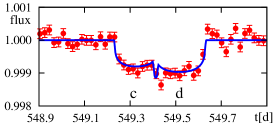
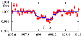
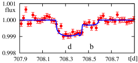
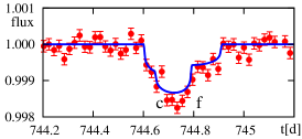
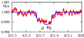
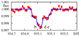
Figure 1 displays a few selected fragments of the data set marked with red dots and error bars which are over-plotted on the synthetic curve best–fitting the data (blue curve). The fitting procedure will be described in more detail in Sect. 2.3. The last panel shows transits of three planets (b, d and e).

2.2 The model of orbital motion

The orbital motion of multiple planetary system is described in terms of the full $N$-body problem in the Poincaré reference frame (e.g., Morbidelli, 2002). In this frame, the Cartesian coordinates of the planets are astrocentric, while their velocities are barycentric. The equations of motion are integrated with the second order symplectic integrator SABA₂ (Wisdom & Holman, 1991; Laskar & Robutel, 2001). It provides 2-3 times better CPU performance than other algorithms, which we tested (like the Bulirsh-Stoer-Gragg scheme, BGS) constrained with the same time–step accuracy. To speed-up the computations even more, we did not integrate the system at all measurements moments. This would force $\sim 30$-minute step-size of the integrator. Instead, we fixed this step-size to $\Delta t\sim 1/20$ of the innermost period of planet b, i.e., $\Delta t\approx 0.5$ day. Furthermore, the flux function $F(t)$ is computed only close to the mid-transits. Ingress and egress times of particular events are tabulated. When a transit takes place, the coordinates of particular planet at time $t$ required to evaluate the flux deficit are determined through the polynomial interpolation on five nodes around $t$. Through a comparison with the direct, full-accuracy integrations with the BGS algorithm, we found that the selected time time-step and the number of interpolation nodes provide a sufficient precision and acceptable CPU overhead. We examined this method by changing the number of nodes in the polynomial interpolation, as well as the time step-size. The flux level, interpolated on five nodes and with $\Delta~{}t\approx 0.5$ day, differs from its exact value by less than $10^{-9}$.

2.3 Optimization algorithm and error estimation

We searched for the best–fit model of the transits by a common minimization of the $\chi_{\nu}^{2}$ function. This function is defined as follows:

$$\chi_{\nu}^{2}={\frac{1}{N_{{\mbox{\scriptsize obs}}}-N_{{\mbox{\scriptsize p}}}-1}\sum_{j=1}^{N_{{\mbox{\scriptsize obs}}}}\frac{1}{\sigma_{j}^{2}}\Big{[}F_{j}-F(t_{j})\Big{]}^{2}},$$ (2)

where $N_{{\mbox{\scriptsize obs}}}$ is the number of observations, $N_{{\mbox{\scriptsize p}}}$ is the number of free parameters, $\nu=N_{{\mbox{\scriptsize obs}}}-N_{{\mbox{\scriptsize p}}}-1$ is the number of the degrees of freedom, $\sigma_{j}$ is the error of the $j$-th observation $F_{j}$, and $F(t_{j})$ is a model function evaluated at time $t_{j}$. This form of the $\chi_{\nu}^{2}$–function is correct if the uncertainties are uncorrelated (see, e.g., Baluev, 2009). To verify whether the available photometric data fulfill this assumption, one has to use a more general statistical model incorporating the red–noise effect. However, under particular settings of our $N$-body photometric model, this would require an enormous CPU overhead. Hence, we use equation 2 as a reasonable first order approximation.

The best–fit parameters of the transits model are searched through a two–step optimization method. In the first step, we apply a robust and well tested quasi-global Genetic Algorithm (GA, see, Charbonneau, 1995; Deb, 2004) which makes it possible to find promising solutions. A local, fast gradient method (here, the Levenberg-Marquardt algorithm) is then used to refine the solutions found in the GA step. Such an approach is called the hybrid optimization (see Goździewski et al., 2008, and references therein). Let us note that the parameter space is huge as it has dimension of 50. Some of these parameters can be determined very well, like the orbital periods of the transiting planets. Unfortunately, due to the relatively short observational time window, many parameters which are critical for the stability (relative inclinations, masses, nodal lines) cannot be well constrained. It makes the fitting process a challenging problem.

The parameter errors are estimated through the bootstrap algorithm (see, e.g., Press et al., 1992). The bootstrap is CPU–demanding, but it is straightforward method to estimate standard errors in high-dimensional problems and for large number of data. The light–curves which we analyzed have $\sim$22,000 points. The bootstrap algorithm requires to find the best–fit solutions to a large number of synthetic sets derived through random sampling with replacement from the original measurements. To obtain reliable error estimates of the best–fit parameters, one needs at least $\sim 10^{3}$–$10^{4}$ synthetic solutions. When such a large set of the best–fit models is gathered, we constructed normalized histograms for each free parameter. These histograms reflect the parameter distribution in response to the errors of the measurements, and may be smoothly approximated by an asymmetric Gaussian function. This makes it possible to determine the standard uncertainties. To perform the bootstrap procedure, at first one needs to find reliable best–fit parameters for the nominal data set. This step was done through an intensive quasi-global search with the help of the hybrid algorithm. The bootstrap computations are CPU-time consuming and were performed on the reef CPU-cluster of the Poznań Supercomputing Centre.

2.4 Numerical setup of the dynamical analysis

In spite of small eccentricities and apparently co-planar orbits, the Kepler-11 systems is orbitally very active. It appears as dynamically packed planetary system (the definition is given in Barnes et al., 2008), with only narrow stable zones in the phase space. For this reason, we used the best-fit model solutions gathered in the bootstrap search as the input data to extensive dynamical study of this system. As we will discuss later, a study of the stability is a challenging problem. Due to relatively short observational window ($\sim 500$ days), weak transits having depths comparable with the measurements errors and a small number of data points covering particular transits (typically $10-15$), the derived initial conditions may be shifted away from the real configurations.

To investigate the dynamics of the Kepler-11 system in a global manner, we applied an approach in our previous papers which is well established in the literature. It relies on reconstructing the structure of the phase space with the fast indicator MEGNO (Cincotta & Simó, 2000; Cincotta et al., 2003). This dynamical characteristic makes it possible to distinguish between regular (stable) and irregular (chaotic, unstable) trajectories in the phase space by computing relatively short numerical orbits. Having representative solutions selected in the bootstrap statistics, we study their neighborhood on the dynamical maps. Constructing a dynamical map relies on two model parameters, e.g., the semi-major axes of a pair of planets. The selected parameters are varied in the given range at a discrete grid. The remaining components of the initial parameter vector are fixed at their nominal values. If it is necessary, they are altered to preserve the observational constraints. Then we calculate MEGNO at each point of the grid. Dynamical maps are informative and become a standard numerical tool helpful to understand the global dynamics of multiple systems.

To compute the MEGNO indicator, we must solve the variational equations to the equations of motion of the planetary $N$-body problem. The Kepler-11 system architecture with low–eccentric orbit and small masses is an ideal target for an efficient symplectic algorithm described in (Goździewski, 2003; Goździewski et al., 2008). The general-purpose integrators, like the Runge-Kutta or Bulirsh-Stoer-Gragg schemes are not efficient nor accurate enough in this case. These methods introduce a systematic drift of the energy and other integrals. To avoid such errors, and to solve the variational equations, we apply the tangent map introduced by Mikkola & Innanen (1999). As the very basic step, it requires to differentiate the “drift” and “kick” maps of the standard leap–frog algorithm. The variations may be then propagated within the same symplectic scheme, as the equations of motion. Having the variational vector ${\boldsymbol{\delta}}$ computed at discrete times, we find temporal $y$ and mean $Y$ of the MEGNO at the $j$-th integrator step $j=1,2,\ldots$, (Cincotta et al., 2003; Goździewski et al., 2008):

$$Y(j) = \frac{(j-1)Y(j-1)+y(j)}{j},$$

$$y(j) = \frac{j-1}{j}y(j-1)+2\ln\left(\frac{\delta_{j}}{\delta_{j-1}}\right)$$

with initial conditions $y(0)=0$, $Y(0)=0$, $\delta=|\,{\boldsymbol{\delta}}\,|$. The MEGNO maps tend asymptotically to

$$Y(j)=ahj+b,$$

where $a=0,b\sim 2$ for quasi-periodic orbits, $a=b=0$ for stable, periodic orbit, and $a=(1/2)\sigma,b=0$ for chaotic orbit with the maximal Lyapunov exponent $\sigma$. The tangent MEGNO map is linear, hence the variational vector can be normalized, if its value grows too large for chaotic orbits. In practice, we stop the integration if the MEGNO indicator reaches a given limit (usually, $Y=5$).

The symplectic maps were propagated with the 4-th order SABA₄ scheme in (Laskar & Robutel, 2001). A choice of the fixed step-size must be carefully controlled. We did this, checking whether the relative energy error is “flat” across the dynamical map (Goździewski et al., 2008) and sufficiently small. Indeed, the step–size $\sim 0.5$ day preserved this error at a level of $10^{-11}$ over the total integration times up to $T\sim 40,0000$ yr ($\sim 100,000$ periods of the outermost planet). This time scale is long enough to detect the most significant 2-body and 3–body MMRs though even such integration period may be insufficient to detect all “dangerous” unstable resonances. Weakly chaotic motions due to multi-body MMRs still may lead to catastrophic events after much longer time (Goździewski et al., 2008).

The dynamical maps in this paper have typical resolution up to $512\times 512$ pixels. This requires an enormous CPU-time. It is basically not possible to perform such intensive computations on a single workstation. Therefore, we used our new Message Passing Interface (MPI) based environment Mechanic (Slonina et al., 2012) to perform the computations in a reasonable time in CPU-clusters. They were performed on the reef cluster at the Poznań Supercomputing Centre. A Mechanic run of a typical dynamical map occupied up to 1200 CPU cores for $\sim 16$ hours.

2.5 Free parameters of the transit model

The free parameters of the transit model are the stellar radius $R_{0}$, the limb darkening coefficients $\gamma_{1},\gamma_{2}$; the mass $m_{i}$, radius $R_{i}$ and orbital elements of each planet in the system, where $i=$b,c,d,e,f,g. Planetary orbits are described through the Poincaré geometric, osculating elements at the epoch of the first observation JD 2455964.51128: a tuple $(a_{i},e_{i},I_{i},\Omega_{i},\omega_{i},\mathcal{M}_{i})$ is for the semi-major axis, eccentricity, inclination to the plane of the sky, the longitude of ascending nodes, the argument of pericenter, and the mean anomaly, respectively. The orbital node of the first planet, $\Omega_{{\mbox{\scriptsize b}}}=0^{\circ}$ due to invariance of the model with respect to a rotation of the whole system. The inclinations are obviously close to $90^{\circ}$. A deviation from $90^{\circ}$ is irrelevant only for single-planet systems.

In a multi-planet system, some orbits may be inclined to the sky plane by angle $\neq 90^{\circ}$, which implies different relative inclinations between orbits of particular planets, even for the same longitudes of nodes. Due to the invariance of transits with respect to the direction of the total angular momentum of the system, a combination of $(I_{i}\leq 90^{\circ},\Omega_{i})$ means the same geometry as $([180^{\circ}-I_{i}]\geq 90^{\circ},-\Omega_{i})$. Thus, when necessary, for a given planet p we can fix the range of $I_{{\mbox{\scriptsize p}}}\leq 90^{\circ}$ and $(I_{i},\Omega_{i})$ are corrected for remaining companions, in accord with the invariance relation.

Orbital elements $(a_{i},e_{i},\omega_{i},\mathcal{M}_{i})$ are not fully suitable for transiting systems with small relative inclinations and small eccentricities. To avoid singularities and weakly constrained elements, like $\omega_{i}$ when $e_{i}=0$ (circular or weakly eccentric orbits), we use the Poincaré modified elements $(X_{i}\equiv e_{i}\cos\omega_{i}$, $Y_{i}\equiv e_{i}\sin\omega_{i})$ instead of $(e_{i},\omega_{i}$).

Similarly, the orbital period $P_{i}$ is more suitable for model fitting than $a_{i}$ since the semi–major axis depends on the planetary mass $m_{i}$ (a free parameter) and on the stellar mass $m_{0}$, which is fixed to $0.95\,\mbox{m}_{\sun}$, but it can be also fitted. Hence, we define $P_{i}$ as one of osculating elements related to $a_{i}$ through the IIIrd Keplerian law.

The mean anomaly $\mathcal{M}_{i}$ strongly depends on $\omega_{i}$. It determines the relative orbital phase (the mean longitude) but is also related to $e_{i}$. This may be avoided by choosing the time of the first transit $T_{i}$ as a free parameter instead of $\mathcal{M}_{i}$, because it is one of the directly determined observables from the light-curves. Simple relations between $T_{i}$ and Poincaré canonical elements may be derived easily.

2.6 Direct and indirect transit model parameters

The direct parameters of the transit model are determined from the basic observables: it is the mean period of transits $P^{*}_{i}$, the depths, duration times of the transits, and shapes of the light-curves (through the limb–darkening coefficients). These data are usually derived from the period–phased light–curves of particular planets. The depths and durations of transit determine the ratio of planetary and stellar radii, $R_{i}/R_{0}$. If the stellar mass $m_{0}$ is fixed then $R_{i}$ and $R_{0}$ may be resolved. We can also determine $I_{i}$ up to the angular momentum direction invariance, and $T_{i}$. In general, the mean period of transit events $P^{*}_{i}$ is different from the osculating orbital period at the epoch of the first observation, $P_{i}$. A shape of the event–period phased light–curves make it possible to fit the limb darkening coefficients, $\gamma_{1},\gamma_{2}$.

These parameters of the transit model are independent on the the $N$-planet dynamics. Hence the remaining are indirect parameters. To resolve them, a dynamical model of the orbital evolution is required. The indirect parameters consist of planetary masses $m_{i}$ as well as orbital elements, $e_{i}$, $\Omega_{i}$, $\omega_{i}$ and $P_{i}$ (instead of $P^{*}_{i}$). Knowing $m_{i}$ and $P_{i}$, we may fix the osculating semi-major axis $a_{i}$ at the date of the first (or prescribed) observation.

We would like to note, that the above distinction for two types of model parameters is somehow arbitrary in our photometric model. In our algorithm both the direct and indirect parameters are fitted simultaneously, unlike, for instance, the TTV algorithm, in which the direct parameters are fitted at the first stage, and the indirect parameters are fitted in the next step.

Usually, the direct parameters can be estimated much more reliably than the indirect parameters. Even a potential derivation of the indirect parameters depend on the particular model of motion. i.e., kinematic — Keplerian, or dynamic — Newtonian, and on the used method of modelling the observations. In the Keplerian (kinematic) model (see, e.g., Agol et al., 2005), mid-transits of a given planet are governed by geometric reflex motion of the star around the center of mass in a sub-system composed of the star and all inner planets. For instance, transits of planet d are affected by planets b and c, but any outer planet does not affect transits of its inner companions. Hence, in accord with the Keplerian model, the indirect parameters $(m_{{\mbox{\scriptsize g}}},a_{{\mbox{\scriptsize g}}},e_{{\mbox{\scriptsize g}}},\Omega_{{\mbox{\scriptsize g}}},\omega_{{\mbox{\scriptsize g}}})$ of the outermost planet g in the Kepler-11 system cannot be determined at all.

In a given pair of planets, the outer companion affects the transits times of the inner planet only through gravitational mutual perturbations which lead to changes of osculating orbital elements. To account for the mutual interactions, one has to apply the self-consistent $N$-body model of motion of the system.

Usually, to resolve the indirect parameters from photometric observations, the well known TTV method is used (Agol et al., 2005). It has two steps. At first, we determine the mean periods, the mid-transits, and then the (O-C) residua, i.e., differences between the measured and ephemeris transit times. The (O-C) variations are observables in the second step during which we search for masses, eccentricities, and arguments of pericenters of planetary companions. The TTV method in this form has a limitation, because it does not make any use of transit depths nor their duration times. If the individual inclinations of planets are different, the planets transit the parent star usually at different attitudes. Hence the transit depths as well as duration times may vary, like the (O-C) of mid-transits. This information can be used to better constrain the transit model.

The mutual inclinations depend on the longitudes of ascending nodes in accord with

$$\cos\Delta I_{i,j}=\cos I_{i}\cos I_{j}-\sin I_{i}\sin I_{j}\cos(\Omega_{i}-\Omega_{j}).$$

Because the inclinations of transiting planets, ($I_{i}$, $I_{j}$) must be close to $90^{\circ}$ then $\Delta I_{i,j}\approx|\Omega_{i}-\Omega_{j}|$. Within this approximation, the TTV method is apparently not sensitive for individual $\Omega_{i}$. In fact, different values of $\Omega_{i}$ imply different mutual inclinations affecting the dynamics and (O-C). However, the dynamical variability of (O-C) due to mutual interactions is weaker than the geometric variability due to changes of transit depths and duration times reflecting the motion of the star around the mass center of the system.

Overall, by direct modeling of the light-curves (photometric measurements), rather than the mid-transit times, we can resolve the (O-C) with an improved precision. Modeling the light-curves in terms of the $N$-body model is CPU-demanding, but it makes it possible to estimate individual longitudes of nodes and mutual inclinations. In particular, as will be shown later, the direct method helped us to derive accurate relative inclinations between planets b and c, as well as between d and e $\sim 2^{\circ}\pm 2^{\circ}$.

3 Results of the bootstrap analysis

We performed the direct bootstrap TTV analysis of a few different orbital models of the Kepler-11 system. In the most general case (I), all parameters discussed in the previous section are the free parameters of the fit model. Some of them are poorly constrained by the observations, in particular, the eccentricity of planet g and particular longitudes of nodes. Therefore, we also studied less general models, in which some of weakly constrained parameters are fixed. In the second model (II), $X_{{\mbox{\scriptsize g}}}=0$, $Y_{{\mbox{\scriptsize g}}}=0$, i.e., $e_{{\mbox{\scriptsize g}}}=0$. In the third model (III), also $\Omega_{{\mbox{\scriptsize g}}}=0^{\circ}$, while in the last model (IV), $\Omega_{{\mbox{\scriptsize b}}},\Omega_{{\mbox{\scriptsize c}}},\Omega_{{\mbox{\scriptsize d}}},\Omega_{{\mbox{\scriptsize e}}},\Omega_{{\mbox{\scriptsize f}}}$ are all fixed at $0^{\circ}$. Because inclinations $I_{i}$ are not exactly equal to $90^{\circ}$, also $\Delta I_{i,j}\geq 0^{\circ}$.

For each of these four transit models, we applied the bootstrap algorithm and we gathered sets of $\sim 1500$ solutions for each instance of the transit model.

3.1 Model I: systems with $\boldsymbol{e_{g}\neq 0}$

Figure 2: Bootstrap histograms for $X_{{\mbox{\scriptsize g}}},Y_{{\mbox{\scriptsize g}}},\Omega_{{\mbox{\scriptsize g}}}$, transit model I. See the text for more detail.

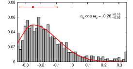
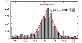
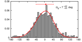
Figure 2 shows an outcome of the bootstrap algorithm in the form of normalized histograms constructed for $X_{{\mbox{\scriptsize g}}},Y_{{\mbox{\scriptsize g}}}$ and $\Omega_{g}$, and depicted from the left to the right panel, respectively. The red solid curves illustrate the best fit asymmetric Gauss function to the histogram bins. The formal $1\sigma$ errors are marked with red bars displayed above the histograms. The best fit parameters corresponding to the maximum of the Gaussian distribution are written in the respective panels, and they may be compared with the nominal solutions given in Table  1. The uncertainties of the eccentricity and longitude of node of planet g are relatively large.

Because the nominal system is dynamically unstable, we examined the whole set of $\sim 1500$ bootstrap solutions by calculating their MEGNO indicator $\langle Y\rangle$ on the time interval of $\sim 8000$ yr. It corresponds to $\sim 25,000$ periods of the most distant companion. Such a characteristic time scale should be long enough to detect unstable solutions due to low–order 2–body and 3–body mean motion resonances (Goździewski et al., 2008, and references therein). Unfortunately, all initial configurations exhibit large values of $\langle Y\rangle$, indicating that the system is strongly chaotic. The main source of instability are crossing orbits in the system, that lead to disruptive events , i.e., one or more of the planets were ejected from the system or collided with the parent star. None of the tested solutions passed the direct integration over 10 Myr.

The parameter space of the Kepler-11 system is $\sim 50$-dimensional, and the dimension of the phase space of the $N$-body model is $36$-dimensional. The $\langle Y\rangle$ experiments indicate that this system can be locally chaotic and its phase space is filled with mostly unstable solutions. Then only small regions of stable MMRs may be present. In the light of a large dimension of the phase space, the gathered statistics of best–fit configurations is still very poor. We conclude that due to short data span of only $\sim 500$  days, and unconstrained elements of the most general model, we cannot find reliably stable solutions assuming the most general transit model I. Unfortunately, in this high–dimensional problem an alternate GAMP algorithm that relies on the optimization with imposed stability constrains (Goździewski et al., 2008) would be CPU-time expensive.

Table 1: Bootstrap results for transit model I. Mass of the star is $0.95\,\mbox{m}_{\sun}$ (fixed). The best-fitting stellar parameters of this model are $R_{0}=1.140^{+0.030}_{-0.027}$, ${\gamma_{1}=0.33^{+0.47}_{-0.30}}$, ${\gamma_{2}=0.41^{+0.24}_{-0.34}}$, $\gamma_{1}+\gamma_{2}=0.74^{+0.23}_{-0.23}$. Osculating Poincaré elements are given at the epoch of the first observation JD 2455964.51128.

parameter/planet	b	c	d	e	f	g
$m\,[\mbox{m}_{\earth}]$	$4.2^{+2.4}_{-3.0}$	$9.2^{+3.8}_{-6.9}$	$8.9^{+3.5}_{-2.7}$	$10.7^{+2.4}_{-2.1}$	$3.6^{+5.4}_{-2.6}$	$18^{+24}_{-15}$
$R\,[\mbox{R}_{\earth}]$	$2.04^{+0.18}_{-0.10}$	$3.25^{+0.13}_{-0.14}$	$3.58^{+0.17}_{-0.14}$	$4.71^{+0.20}_{-0.18}$	$2.82^{+0.19}_{-0.14}$	$3.80^{+0.15}_{-0.14}$
$\bar{\rho}\,[\bar{\rho}_{\earth}]$	$0.50^{+0.38}_{-0.29}$	$0.27^{+0.14}_{-0.17}$	$0.19^{+0.07}_{-0.07}$	$0.10^{+0.04}_{-0.02}$	$0.16^{+0.22}_{-0.14}$	$0.33^{+0.47}_{-0.23}$
$a\,[\mbox{au}]$	$0.091089\left({}^{+13}_{-11}\right)$	$0.106522\left({}^{+7}_{-12}\right)$	$0.154241\left({}^{+19}_{-10}\right)$	$0.193937\left({}^{+15}_{-21}\right)$	$0.249489\left({}^{+39}_{-25}\right)$	$0.463918\left({}^{+59}_{-28}\right)$
$e\,\cos\omega$	$0.010^{+0.017}_{-0.021}$	$0.005^{+0.017}_{-0.018}$	$-0.013^{+0.008}_{-0.022}$	$-0.020^{+0.008}_{-0.022}$	$-0.006^{+0.011}_{-0.018}$	$-0.26^{+0.16}_{-0.08}$
$e\,\sin\omega$	$-0.011^{+0.031}_{-0.025}$	$-0.004^{+0.028}_{-0.020}$	$-0.009^{+0.006}_{-0.015}$	$-0.016^{+0.007}_{-0.011}$	$-0.017^{+0.016}_{-0.021}$	$0.008^{+0.058}_{-0.085}$
$I^{*}\,$ [deg]	$88.40^{+0.76}_{-0.42}$	$91.17^{+0.40}_{-0.20}$	$89.18^{+0.22}_{-0.17}$	$88.743^{+0.062}_{-0.060}$	$89.30^{+0.12}_{-0.09}$	$90.23^{+0.16}_{-0.11}$
$\Omega\,$ [deg]	$0$ (fixed)	$3.2^{+4.2}_{-2.9}$	$-33^{+13}_{-11}$	$-31^{+12}_{-11}$	$-32^{+30}_{-27}$	$-65^{+51}_{-46}$
$\mathcal{M}+\omega\,$ [deg]	$204.5^{+2.2}_{-2.5}$	$265.3^{+2.0}_{-2.0}$	$182.8^{+2.3}_{-1.0}$	$197.4^{+1.8}_{-1.4}$	$89.5^{+1.5}_{-1.8}$	$6^{+7}_{-19}$
$P\,[\mbox{d}]$	$10.3023\left({}^{+24}_{-18}\right)$	$13.0284\left({}^{+12}_{-20}\right)$	$22.7002\left({}^{+41}_{-24}\right)$	$32.0051\left({}^{+42}_{-46}\right)$	$46.700\left({}^{+11}_{-6}\right)$	$118.410\left({}^{+16}_{-10}\right)$
$T_{0}\,[\mbox{JD}]$	$471.505\left({}^{+20}_{-7}\right)$	$471.175\left({}^{+20}_{-4}\right)$	$481.455\left({}^{+16}_{-6}\right)$	$487.178\left({}^{+22}_{-8}\right)$	$464.673\left({}^{+15}_{-8}\right)$	$501.916\left({}^{+42}_{-21}\right)$

3.2 Transit model II: systems with $\boldsymbol{e_{g}=0}$

In the next model, we narrow the mostly unconstrained parameters of the transit model. We fix the eccentricity $e_{g}=0$, hence $X_{{\mbox{\scriptsize g}}}$ and $Y_{{\mbox{\scriptsize g}}}$ are both equal to $0$. The results of the bootstrap algorithm are illustrated in Figs. 3-9. All panels in these figures are constructed in the same manner as Fig. 2. We tested, whether the best–fit parameters encompass at least marginally stable solutions with $\langle Y\rangle\approx 2$ after $T=16000$ yr.

Figure 3: Bootstrap histograms for planetary masses, transit model II.

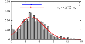
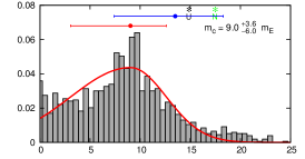
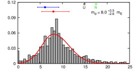
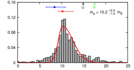
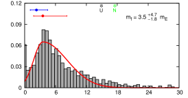
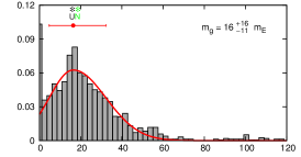
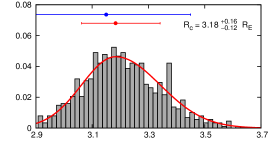
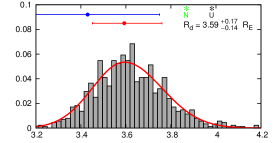
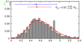
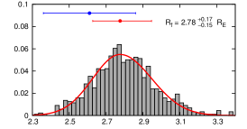
Figure 3 shows the normalized histograms for masses of particular planets expressed in the Earth masses. Besides formal uncertainties obtained through the bootstrap (filled red circles), the best-fit parameters derived in (Lissauer et al., 2011) are plotted (blue filled circles). Clearly, these estimates coincide very well in both cases. There is one exception though, since the mass of planet g is not resolved in Lissauer et al. (2011). The direct code helps to resolve also this mass. It is constrained surprisingly well, in spite of a narrow observational window. This result confirms our predictions. Because the orbital model is constrained by all measurements, not the TTVs only, the direct algorithm makes use of dynamical information contained in the transit depths and widths.

For a reference, black and green asterisks in Fig. 3 mark masses of the Uranus and Neptune, respectively. The masses of planets b and f appear in a range specific for the super-Earths. They are significantly smaller than the masses of two most distant planets in our Solar system but, as we will show in the next section, their chemical composition has likely much common with the ice giants in the Solar system.

Figure 4: Bootstrap histograms for the planetary radii, transit model II.

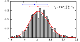
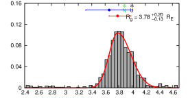
The next Fig. 4 shows histograms constructed for planetary radii expressed in the unit of the Earth radius. These results confirm data in the discovery paper. Similarly to the previous plots, the radii of Uranus and Neptune are marked with asterisks. They are also labeled with $\mbox{R}_{{\mbox{\scriptsize U}}}$ and $\mbox{R}_{{\mbox{\scriptsize N}}}$, respectively. The derived radius of planet g confirms a hypothesis that it may belong to the Uranus/Neptune–class. We note that most of the planets has radii smaller than $\mbox{R}_{{\mbox{\scriptsize U/N}}}$, and only planet e has its radius larger.

Figure 5: Bootstrap histograms for the mean densities, transit model II.

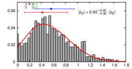
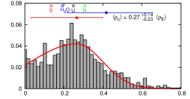
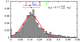
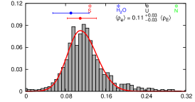
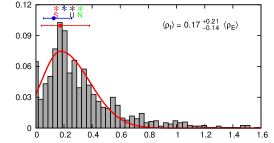
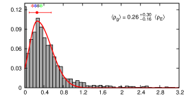
Histograms of the mean densities are presented in Fig.  5. The $x$-axis is for the density expressed w.r.t. the Earth density. Black and green asterisks mark the values characteristic for Uranus and Neptune, respectively. The mean densities of Saturn and water are also marked with the red and blue symbols, respectively. According to this plot, the less dense planet e has a density of Saturn. The most dense planet b may be almost as dense as the Earth. The densities of the other planets span a range characteristic for Saturn and Neptune, from $\rho_{{\mbox{\scriptsize S}}}$ to $\rho_{{\mbox{\scriptsize N}}}$.

Figure 6: Bootstrap histograms for the semi-major axes, transit model II.

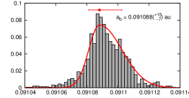
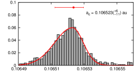
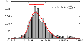
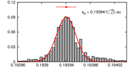
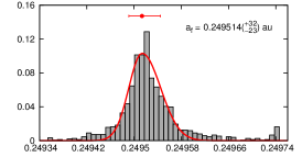
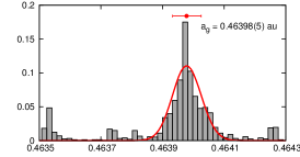
Figure 6 is for the bootstrap histograms constructed of the semi-major axes. These parameters are the best determined among all of the transit models, with uncertainties of the order of $10^{-5}\,\mbox{au}$ only. We do not compare these results with data in (Lissauer et al., 2011) because they accounted for the formal error of the stellar mass. Note that we fixed $m_{0}=0.95\,\mbox{m}_{\sun}$, because we found that this parameter is unconstrained by the photometric data. Yet it seems that the $\chi_{\nu}^{2}(m_{0})$ function monotonically increases in the range of $m_{0}\in(0.7,1.2)\,\mbox{m}_{\sun}$.

Figure 7: Bootstrap histograms for eccentricities and $\Delta\omega_{{\mbox{\scriptsize b}},{\mbox{\scriptsize c}}}$, transit model II.

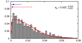
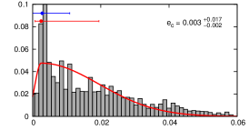
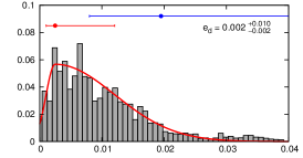
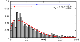
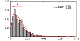
The first five panels of Fig. 7 are for the eccentricities, and the bottom, right-hand panel is for $\Delta\omega_{{\mbox{\scriptsize b}},{\mbox{\scriptsize c}}}\equiv\omega_{{\mbox{\scriptsize b}}}-\omega_{{\mbox{\scriptsize c}}}$ . These histograms confirm that the eccentricities of planets b to f are small, typically less that $0.05$, and the arguments of pericenters are not well constrained. The last panel assures us that $\Delta\omega_{{\mbox{\scriptsize b}},{\mbox{\scriptsize c}}}$ is determined with an error of only $\sim 10^{\circ}$, recalling a narrow time–window of the photometric data. The best–fit parameters of model II are given in Tab. 2.

Table 2: Bootstrap results for model II (with fixed $e_{g}=0$). Mass of the star is $0.95\,\mbox{m}_{\sun}$ (fixed). Best fitted stellar parameters are $R_{0}=1.161^{+0.035}_{-0.028}$, ${\gamma_{1}=0.32^{+0.46}_{-0.30}}$, ${\gamma_{2}=0.41^{+0.17}_{-0.36}}$, $\gamma_{1}+\gamma_{2}=0.73^{+0.16}_{-0.30}$. Osculating Poincaré elements are given at the epoch of the first observation JD 2455964.51128.

parameter/planet	b	c	d	e	f	g
$m\,[\mbox{m}_{\earth}]$	$4.2^{+2.8}_{-2.4}$	$9.2^{+3.6}_{-6.0}$	$9.2^{+3.5}_{-2.6}$	$10.5^{+2.4}_{-1.0}$	$4.4^{+4.7}_{-1.8}$	$3^{+16}_{-3}$
$R\,[\mbox{R}_{\earth}]$	$2.07^{+0.16}_{-0.13}$	$3.31^{+0.16}_{-0.12}$	$3.65^{+0.17}_{-0.14}$	$4.80^{+0.30}_{-0.19}$	$2.88^{+0.17}_{-0.15}$	$3.93^{+0.20}_{-0.13}$
$\bar{\rho}\,[\bar{\rho}_{\earth}]$	$0.48^{+0.42}_{-0.30}$	$0.25^{+0.14}_{-0.23}$	$0.19^{+0.07}_{-0.07}$	$0.10^{+0.03}_{-0.03}$	$0.19^{+0.21}_{-0.14}$	$0.04^{+0.30}_{-0.04}$
$a\,[\mbox{au}]$	$0.091087\left({}^{+15}_{-7}\right)$	$0.106521\left({}^{+6}_{-11}\right)$	$0.154233\left({}^{+16}_{-10}\right)$	$0.193926\left({}^{+16}_{-17}\right)$	$0.249511\left({}^{+32}_{-23}\right)$	$0.463924\left({}^{+42}_{-37}\right)$
$e\,\cos\omega$	$0.006^{+0.011}_{-0.022}$	$0.001^{+0.010}_{-0.017}$	$-0.013^{+0.007}_{-0.019}$	$-0.020^{+0.007}_{-0.015}$	$-0.004^{+0.016}_{-0.013}$	$0$ (fixed)
$e\,\sin\omega$	$0.020^{+0.027}_{-0.027}$	$0.024^{+0.025}_{-0.023}$	$0.008^{+0.008}_{-0.015}$	$-0.002^{+0.005}_{-0.014}$	$-0.007^{+0.020}_{-0.016}$	$0$ (fixed)
$I^{*}\,$ [deg]	$88.39^{+0.95}_{-0.24}$	$91.17^{+0.38}_{-0.22}$	$89.14^{+0.23}_{-0.13}$	$88.701^{+0.052}_{-0.076}$	$89.282^{+0.09}_{-0.11}$	$90.31^{+0.086}_{-0.055}$
$\Omega\,$ [deg]	$0$ (fixed)	$3.4^{+4.3}_{-2.7}$	$-23^{+12}_{-12}$	$-22^{+11}_{-12}$	$-25^{+24}_{-27}$	$37^{+63}_{-59}$
$\mathcal{M}+\omega\,$ [deg]	$205.0^{+2.2}_{-2.3}$	$265.7^{+2.1}_{-1.2}$	$182.7^{+1.9}_{-0.9}$	$197.4^{+1.6}_{-1.0}$	$89.2^{+1.7}_{-1.5}$	$336.282^{+0.049}_{-0.093}$
$P\,[\mbox{d}]$	$10.3019\left({}^{+23}_{-14}\right)$	$13.0281\left({}^{+14}_{-18}\right)$	$22.6985\left({}^{+34}_{-22}\right)$	$32.0025\left({}^{+45}_{-34}\right)$	$46.7054\left({}^{+89}_{-57}\right)$	$118.4147\left({}^{+90}_{-33}\right)$
$T_{0}\,[\mbox{JD}]$	$471.504\left({}^{+21}_{-7}\right)$	$471.176\left({}^{+18}_{-4}\right)$	$481.454\left({}^{+14}_{-6}\right)$	$487.177\left({}^{+19}_{-9}\right)$	$464.670\left({}^{+14}_{-9}\right)$	$501.916\left({}^{+40}_{-11}\right)$

Inclination $I_{{\mbox{\scriptsize b}}}$ was constrained to the $\leq 90^{\circ}$ range, and due to the invariance rule implied by the direction of the total angular momentum, the remaining inclination $I_{i}$ may be smaller and larger than $90^{\circ}$. We tested whether there is a correlation of the transit events with a given half–disc of the star. We found that both cases are equally possible. Because the orbits are inclined to the plane of the sky at angles close to $90^{\circ}$, the relative inclinations with the same longitudes of nodes may be $\sim 2^{\circ}$–$3^{\circ}$. As expected, the indirect parameters $\Omega_{i}$ are unconstrained, see Tab. 2. Therefore, the main contribution to the uncertainties of the relative inclinations comes from ambiguous estimates of $\Omega_{i}$ rather than of $I_{i}$.

Figure 8: Bootstrap histograms for absolute inclinations, transit model II.

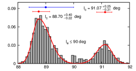
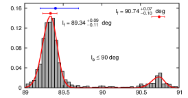
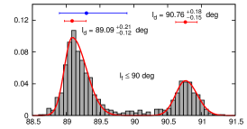
Curiously, there appears a clear correlation between mutual inclinations in particular pairs of orbits, namely c and e, f and e, as well as d and f. This can be seen in normalized histograms constructed for the inclinations, Fig. 8. For a chosen planet, we transform $I_{i}$ to $\leq 90^{\circ}$ range (in accord with the inclination invariance rule), and we compute the bootstrap histogram for $I_{j}$. Panels of Fig. 8, from the left to the right, are for pairs $(i,j)=(\mbox{e},\mbox{c}),(\mbox{e},\mbox{f}),(\mbox{f},\mbox{d})$. If $I_{{\mbox{\scriptsize e}}}\leq 90^{\circ}$ then much more likely $I_{{\mbox{\scriptsize c}}},I_{{\mbox{\scriptsize f}}}\leq 90^{\circ}$ than $I_{{\mbox{\scriptsize c}}},I_{{\mbox{\scriptsize f}}}\geq 90^{\circ}$. Similarly, if $I_{{\mbox{\scriptsize f}}}\leq 90^{\circ}$, then $I_{{\mbox{\scriptsize d}}}\leq 90^{\circ}$ appears more likely than $I_{{\mbox{\scriptsize f}}}\geq 90^{\circ}$.

Table 3: Bootstrap results for model III ($e_{g}=0,\Omega_{g}=0$). Mass of the star is $0.95\,\mbox{m}_{\sun}$ (fixed). Fitted stellar parameters: $R_{0}=1.158^{+0.021}_{-0.038}$, ${\gamma_{1}=0.32^{+0.44}_{-0.25}}$, ${\gamma_{2}=0.41^{+0.25}_{-0.40}}$, $\gamma_{1}+\gamma_{2}=0.73^{+0.32}_{-0.21}$. Osculating Poincaré elements are given at the epoch of the first observation JD 2455964.51128.

parameter/planet	b	c	d	e	f	g
$m\,[\mbox{m}_{\earth}]$	$4.0^{+2.5}_{-3.0}$	$9.1^{+3.3}_{-6.1}$	$9.1^{+3.5}_{-2.9}$	$10.6^{+2.9}_{-2.1}$	$4.3^{+5.8}_{-2.7}$	$1^{+28}_{-1}$
$R\,[\mbox{R}_{\earth}]$	$2.07^{+0.13}_{-0.13}$	$3.30^{+0.13}_{-0.13}$	$3.64^{+0.14}_{-0.16}$	$4.79^{+0.19}_{-0.20}$	$2.88^{+0.17}_{-0.15}$	$3.92^{+0.12}_{-0.15}$
$\bar{\rho}\,[\bar{\rho}_{\earth}]$	$0.45^{+0.40}_{-0.33}$	$0.25^{+0.12}_{-0.17}$	$0.19^{+0.09}_{-0.07}$	$0.10^{+0.05}_{-0.02}$	$0.18^{+0.27}_{-0.09}$	$0.02^{+0.49}_{-0.04}$
$a\,[\mbox{au}]$	$0.091088\left({}^{+15}_{-9}\right)$	$0.106519\left({}^{+9}_{-10}\right)$	$0.154234\left({}^{+22}_{-6}\right)$	$0.193924\left({}^{+24}_{-13}\right)$	$0.249511\left({}^{+31}_{-23}\right)$	$0.463917\left({}^{+55}_{-36}\right)$
$e\,\cos\omega$	$0.015^{+0.013}_{-0.025}$	$0.008^{+0.015}_{-0.017}$	$-0.008^{+0.010}_{-0.016}$	$-0.015^{+0.009}_{-0.011}$	$-0.002^{+0.012}_{-0.015}$	$0$ (fixed)
$e\,\sin\omega$	$0.007^{+0.034}_{-0.019}$	$0.012^{+0.025}_{-0.022}$	$0.000^{+0.007}_{-0.013}$	$-0.010^{+0.005}_{-0.013}$	$-0.011^{+0.016}_{-0.023}$	$0$ (fixed)
$I^{*}\,$ [deg]	$88.35^{+0.83}_{-0.45}$	$88.80^{+0.38}_{-0.20}$	$90.88^{+0.20}_{-0.14}$	$88.701^{+0.071}_{-0.066}$	$89.26^{+0.10}_{-0.12}$	$89.699^{+0.077}_{-0.064}$
$\Omega\,$ [deg]	$0$ (fixed)	$-3.5^{+4.2}_{-2.5}$	$21^{+14}_{-12}$	$20^{+14}_{-11}$	$22^{+24}_{-23}$	$0$ (fixed)
$\mathcal{M}+\omega\,$ [deg]	$204.0^{+2.8}_{-1.7}$	$264.9^{+1.9}_{-1.8}$	$182.2^{+1.5}_{-1.2}$	$196.7^{+1.3}_{-1.2}$	$89.0^{+1.9}_{-1.6}$	$336.29^{+0.05}_{-0.13}$
$P\,[\mbox{d}]$	$10.3020\left({}^{+25}_{-15}\right)$	$13.0278\left({}^{+16}_{-18}\right)$	$22.6986\left({}^{+43}_{-18}\right)$	$32.0019\left({}^{+49}_{-34}\right)$	$46.7056\left({}^{+87}_{-55}\right)$	$118.412\left({}^{+26}_{-12}\right)$
$T_{0}\,[\mbox{JD}]$	$471.504\left({}^{+20}_{-9}\right)$	$471.176\left({}^{+17}_{-4}\right)$	$481.454\left({}^{+17}_{-6}\right)$	$487.176\left({}^{+21}_{-6}\right)$	$464.671\left({}^{+13}_{-10}\right)$	$501.915\left({}^{+43}_{-14}\right)$

Figure 9: Bootstrap histograms for the mutual inclinations, transit model II.

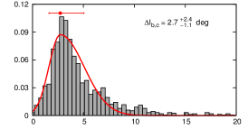
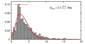
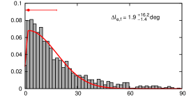
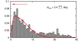
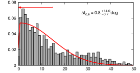
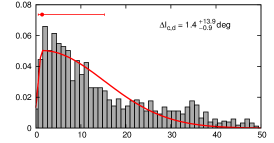
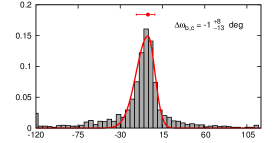
For particular pairs of planets, the relative inclinations can be determined surprisingly well. Figure 9 shows the bootstrap histograms $\Delta I_{i,j}$ for such pairs which exhibit well constrained values. These histograms reveal that orbits of planets b and c are almost coplanar. Similarly, the pair of planets d and e form an almost coplanar sub-system. The mutual inclinations of orbits in these pairs are less than $5^{\circ}$, with most likely values of $2^{\circ}$–$3^{\circ}$. The remaining panels indicate that the mutual inclinations between five inner orbits remain within a few degrees range. Their upper limits are not so small as in the first two sub-systems. The outermost orbit of planet g may by highly inclined to the rest of the system, see errors of $\Omega_{g}$ in Tab. 2.

These results confirm a hypothesis in the discovery paper. In accord with this work, planetary orbits in the Kepler–11 system should be mutually inclined by no more than a few degrees. It flows from estimating a probability that for a given orientation of the orbits, all six planets transit the star. This reasoning assumes that all inclinations are independent. However, we found that Kepler–11 system is composed of two or three sub-systems, which exhibit small mutual inclinations of orbits. Although a probability that the mutual inclinations between these sub-systems are significant seems a bit larger than for fully independent orbits, it still remains very small. We estimate that a randomly located observer can detect transits of all 6 planets with a probability as small as $\sim 0.05\%$, for both models I and II.

Table 4: Bootstrap results for model IV ($e_{g}=0,\Omega_{i}=0,i=b,c,d,e,f,g$). Mass of the star is $0.95\,\mbox{m}_{\sun}$ (fixed). The best–fit stellar parameters: $R_{0}=1.140^{+0.026}_{-0.024}$, ${\gamma_{1}=0.30^{+0.32}_{-0.30}}$, ${\gamma_{2}=0.42^{+0.18}_{-0.42}}$, $\gamma_{1}+\gamma_{2}=0.72^{+0.22}_{-0.25}$. Osculating Poincaré elements are given at the epoch of the first observation JD 2455964.51128.

parameter/planet	b	c	d	e	f	g
$m\,[\mbox{m}_{\earth}]$	$3.3^{+2.4}_{-1.8}$	$8.8^{+4.0}_{-5.0}$	$8.9^{+2.3}_{-3.4}$	$10.3^{+1.9}_{-1.5}$	$4.1^{+3.8}_{-2.4}$	$<21$
$R\,[\mbox{R}_{\earth}]$	$2.01^{+0.13}_{-0.13}$	$3.23^{+0.12}_{-0.12}$	$3.59^{+0.15}_{-0.13}$	$4.70^{+0.21}_{-0.15}$	$2.82^{+0.15}_{-0.15}$	$3.85^{+0.12}_{-0.12}$
$\bar{\rho}\,[\bar{\rho}_{\earth}]$	$0.40^{+0.33}_{-0.19}$	$0.26^{+0.13}_{-0.18}$	$0.19^{+0.07}_{-0.08}$	$0.10^{+0.03}_{-0.03}$	$0.18^{+0.20}_{-0.10}$	$<0.35$
$a\,[\mbox{au}]$	$0.091088\left({}^{+13}_{-11}\right)$	$0.106514\left({}^{+6}_{-8}\right)$	$0.154234\left({}^{+18}_{-7}\right)$	$0.193927\left({}^{+19}_{-10}\right)$	$0.249507\left({}^{+35}_{-26}\right)$	$0.463913\left({}^{+57}_{-39}\right)$
$e\,\cos\omega$	$-0.002^{+0.015}_{-0.021}$	$-0.006^{+0.015}_{-0.016}$	$-0.012^{+0.009}_{-0.019}$	$-0.018^{+0.006}_{-0.017}$	$-0.007^{+0.015}_{-0.020}$	$0$ (fixed)
$e\,\sin\omega$	$0.049^{+0.020}_{-0.050}$	$0.050^{+0.020}_{-0.044}$	$-0.010^{+0.008}_{-0.018}$	$-0.016^{+0.006}_{-0.017}$	$-0.017^{+0.011}_{-0.021}$	$0$ (fixed)
$I^{*}\,$ [deg]	$88.76^{+0.96}_{-0.41}$	$91.00^{+0.40}_{-0.25}$	$90.89^{+0.17}_{-0.18}$	$88.743^{+0.043}_{-0.049}$	$89.30^{+0.10}_{-0.09}$	$89.719^{+0.061}_{-0.068}$
$\mathcal{M}+\omega\,$ [deg]	$205.8^{+2.4}_{-2.1}$	$266.4^{+1.7}_{-1.9}$	$182.7^{+2.1}_{-1.2}$	$197.2^{+1.8}_{-0.9}$	$89.6^{+2.6}_{-1.3}$	$336.286^{+0.066}_{-0.057}$
$P\,[\mbox{d}]$	$10.3021\left({}^{+24}_{-18}\right)$	$13.0269\left({}^{+10}_{-17}\right)$	$22.6986\left({}^{+43}_{-13}\right)$	$32.0027\left({}^{+41}_{-30}\right)$	$46.7044\left({}^{+88}_{-59}\right)$	$118.411\left({}^{+14}_{-15}\right)$
$T_{0}\,[\mbox{JD}]$	$471.505\left({}^{+20}_{-7}\right)$	$471.177\left({}^{+18}_{-3}\right)$	$481.452\left({}^{+17}_{-6}\right)$	$487.176\left({}^{+22}_{-6}\right)$	$464.670\left({}^{+14}_{-9}\right)$	$501.914\left({}^{+26}_{-11}\right)$

3.3 Models III ($\boldsymbol{e_{g}=0,\Omega_{g}=0}$) and IV ($\boldsymbol{e_{g}=0,\Omega_{i}=0}$)

The results for model III and model IV are given in Tabs. 3 and 4. Most of these results are common for all transit models I to IV. There are some differences regarding a determination of the mass of planet g. In the realm of models III and IV (note that both have fixed $e_{g}=0$ and $\Omega_{g}=0$), only an upper limit of $m_{g}$ smaller than $20-30$ Earth masses may be found. The low limits of $m_{g}$ in model I are likely due to weakly constrained $e_{g}$ and $\Omega_{g}$.

Let us recall that in the bootstrap set derived for model II, we found only two solutions with $\langle Y\rangle\approx 2$ after $16000$ yr. However, this integration time scale is too short to detect weak instability which actually leads to catastrophic disruption of these configurations. It was verified by the direct, long–term integrations. Hence, we did not detect any long–term stable configuration in the bootstrap set of model II. Similarly, stability tests performed for configurations of model III did not reveal any stable models. As compared to model II, fixed $\Omega_{{\mbox{\scriptsize g}}}=0$ seem does not change the general view of the stability of the system.

For model IV we found many stable configurations which confirm stability analysis in Lissauer et al. (2011). They found some stable solutions assuming that the Kepler-11 system is strictly co-planar. We may conclude that a factor of small relative inclinations is more important for maintaining the long term stability than small eccentricities. This will be discussed in more detail further in this work.

We examined a probability that a randomly located observer could detect transits of all planets in the system. This is basically unlikely for model III ($\sim 0.09\%$), while for model IV a probability of such an event is larger, and we estimate it $\sim 3.4\%$.

4 Discussion on the planet interiors

Figure 10: The top row: mass, radius and mean density as a function of the semi-major axis (model II). Black and green solid curves are for Uranus and Neptune, respectively. The bottom row: mass–radius, mass–mean density and radius–mean density relations.

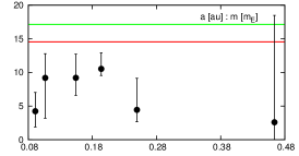
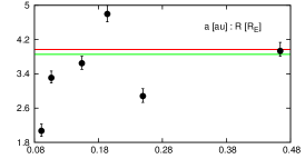
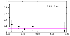
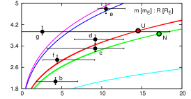
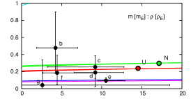
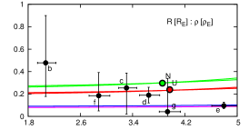
Figure 10 shows bootstrap diagrams of a few selected pairs of parameters. These results are for model II. The top row is for the semi-major axes and the planetary masses, the radii and mean densities, respectively. The red and green curves mark the data for Uranus and Neptune. The bottom row is for the mass–radius, mass–density and radius–density relations, respectively. Similarly, the red and green filled circles are for Uranus and Neptune. As we concluded above, the orbital solutions in set II are only marginally stable, however, it is a matter of unconstrained orbital angles. Note that a discussion in this Section concerns semi-major axes (known with an excellent precision) as well as planetary masses and radii.

This figure reveals that the most inner four planets in the Kepler-11 system exhibit a clear and curious anti/correlation of masses, radii and densities with the semi-major axes. Masses and radii increase with $a_{i}$, while densities decrease. The last panel constructed for $(R,\rho)$ shows a weak anti-correlation between the radii and densities, the smaller radius, the larger density.

Figure 11: Characteristic density $\rho_{0}$ of the chemical mixture of planetary interiors as functions of the mean number of nucleons per one electron, $\mu_{e}$ (model II).

The determined masses and radii of the planets provide some insight into their chemical composition. We use a simple analytic relation between the radius and the mass of a cold body (Lynden-Bell & O’Dwyer, 2001; Lynden-Bell & Tout, 2001) to estimate the characteristic density $\rho_{0}$ of planetary matter. This density can be compared with $\rho_{0}$ calculated for a given number of nucleons per number of electrons of a chemical mixture forming the planet, $\mu_{e}$. The value of $\mu_{e}$ is a simple mean over the elements in each chemical substance or component. For instance the H-He mixture has $\mu_{e}=8/7$ for the mass proportions $3$ to $1$, and ice or rock has $\mu_{e}\approx 2$. In this way, we can obtain some insight into likely chemical composition of the planets.

Our results for Kepler-11 are presented in Fig. 11. Black curves with grey areas are for $\rho_{0}$ and its uncertainty $\Delta\rho_{0}$. Each panel is for one planet of the Kepler-11 system. Data for planets b to planet g are displayed from the left to the right, respectively. The colored curves are for the Solar system, i.e., for Uranus (red), Neptune (green), Jupiter (blue), Saturn (violet) and the Earth (light blue). The density $\rho_{0}$ was computed in a wide range of $\mu_{e}\in[1,2]$. These values are known relatively well for the Sun companions. Following Helled et al. (2011), for Uranus and Neptune one finds $\mu_{e}\approx 1.1$ (for the icy model) and $\mu_{e}\approx 1.35$ (for the rocky model). The density $\rho_{0}$ in these particular case is plotted with filled circles. Similarly, for Jupiter and Saturn, $\mu_{e}$ may be also estimated $\approx 1.08-1.09$ (Guillot, 1999). Values of $\rho_{0}$ for these particular $\mu_{e}$ are marked with circles. Let us note that densities $\rho_{0}$ of Jupiter and Saturn are almost identical.

Lynden-Bell & Tout (2001) argue that $\rho_{0}$ is the zero–pressure density $\rho_{0,{\mbox{\scriptsize p}}}$ of the chemical mixture of the planets. Because their model has many simplifications, $\rho_{0}$ is usually $2-5$ times larger then $\rho_{0,{\mbox{\scriptsize p}}}$. Keeping this in mind, the densities $\rho_{0}$ calculated for Kepler-11 planets can be compared with those of the Solar system planets. The value of $\rho_{0}$ is best determined for planet e. Its is very close to the Jupiter/Saturn (J/S) value $\sim 0.45\,\mbox{g}\,\mbox{cm}^{-3}$. This suggests, that planet e is built mainly of a H/He mixture with mass proportions of the elements close to $3/1$ with a portion of heavier elements contained in ices or rocks. This makes the planet classified as a smaller “cousin” of Jupiter and Saturn rather than of Neptune and Uranus, as suggested in (Lissauer et al., 2011).

The density $\rho_{0}$ of planet b is determined worse than for planet e. It is rather unlikely though that it belongs to the same class as planet e. Parameter $\rho_{0}$ is larger than for Jupiter and Saturn, even taking into account a large uncertainty. It is also larger than $\rho_{0}$ for Uranus and Neptune (U/N)–like planets but is smaller than $\rho_{0}$ for the Earth. We can conclude that planet b is a small planet containing a large percentage of heavy elements in its interior, which is likely larger than in the ice giants. It is reasonable to classify this planet in the super-Earths family, although, it may be also a small Neptune–like planet.

Planet f has the mass similar to planet b. However, its composition is likely between the Jupiter–Saturn and Uranus–Neptune classes. Planet d has likely similar composition as planet f. The best-fit estimate of $\rho_{0}$ for planet c is very close to the Uranus/Neptune value. For planet g there is only the upper limit of $\rho_{0}$. However, it is probably close to the Jupiter/Saturn value or, less likely, to the Neptune/Uranus value.

These conclusions are reinforced after inspecting the bottom-left panel of Fig. 10 illustrating the mass–radius diagram for the Kepler-11 system. The mass–radius relation computed for $\rho_{0}$ and $\mu_{e}$ of the Solar system planets are plotted with different colors. Data are shown for Uranus (red), Neptune (green), Jupiter (blue), Saturn (violet) and Earth (light blue), respectively. Representations of this relation are plotted in the mass-density diagram (the middle panel) and the radius–density diagram (the right panel).

For small masses, the characteristic density $\rho_{0}$ is very close to $\rho$ (see Eq. 34 in Lynden-Bell & O’Dwyer, 2001). This derived decay of $\rho$ with the mean distance from the star suggests that the inner planets may contain larger amount of heavy elements than more distant companions. If this correlation can be confirmed, it may provide an observational constraint for the planet formation theory. Allowing for some speculations here, let us note that all Kepler-11 planets exhibit masses in the same range of a few Earth masses. Hence, they likely have formed in a similar way and physical environment (Rogers et al., 2011). Small eccentricities and small relative inclinations suggest that the system evolved orbitally smoothly towards the current state, conserving the ordering of initial distances from the star. The observed relation between $\rho_{0}$ and $a_{i}$ may then indicate the chemical composition and mass density distribution in the primordial protoplanetary disk.

We underline that the results in this section must be considered as preliminary. Due to relatively narrow time–window of the photometric data, masses of the planets are determined with large uncertainties.

5 Results of the dynamical analysis

The best–fit solutions gathered with the help of the bootstrap algorithm provide us primary information required to perform extensive study of the dynamical stability of the system. Because the orbits of Kepler-11 super-Earth planets are confined within the mean distance of Mercury in the Solar system, we could expect that the dynamics of this system are extremely complex. Indeed, preliminary integrations demonstrated that the Kepler-11 system is dynamically packed, in accord with a definition and the PPS hypothesis in (Barnes et al., 2008). In spite of apparently ordered configurations with quasi–circular, almost coplanar orbits, and relatively small masses, no long-term stable model I solutions were found. Below, we try to resolve this paradox and we try to detect sources of this seemingly odd and strong instability. To illustrate the structure of the phase space close to the best–fit configurations, we choose a few representative solutions and we construct the MEGNO maps in their vicinity.

5.1 Quasi-stable solutions in transit model II

For model II, among $\sim 1500$ initial conditions, we found only 2 configurations exhibiting MEGNO close to $2$ after $T=16000$ yr. Parameters of these solutions are listed in Tabs. 5 and 6.

Table 5: Orbital parameters of marginally stable configuration IIa. Mass of the star is $0.95\,\mbox{m}_{\sun}$. Osculating Poincaré elements are given at the initial epoch JD 2455964.51128.

parameter/planet	b	c	d	e	f	g
$m\,[\mbox{m}_{\earth}]$	$4.550$	$1.542$	$7.224$	$15.698$	$4.340$	$18.530$
$a\,[\mbox{au}]$	$0.091097$	$0.106515$	$0.154241$	$0.193939$	$0.249532$	$0.463815$
$e$	$0.00800$	$0.00698$	$0.00918$	$0.00924$	$0.01827$	$0$ (fixed)
$I\,$ [deg]	$89.048$	$88.938$	$89.023$	$88.803$	$89.339$	$89.470$
$\Omega\,$ [deg]	$0$ (fixed)	$2.119$	$15.216$	$14.804$	$20.626$	$52.574$
$\omega\,$ [deg]	$158.534$	$138.150$	$61.831$	$183.853$	$296.192$	$0$ (fixed)
$\mathcal{M}\,$ [deg]	$47.28591$	$128.23248$	$118.94929$	$12.27874$	$151.62481$	$336.22407$

The first stable solution (refereed to as IIa from hereafter, see Tab. 5), has a relatively low mass of planet c $\sim 1.5$ Earth masses. Two innermost planets b and c have almost coplanar orbits. The next three planets, d, e and f also form a nearly coplanar sub-system (d-e-f), which is inclined to the first two orbits by large angle $\sim 15^{\circ}$. The outermost orbit is inclined even more, by $\sim 50^{\circ}$ to the inner subsystem of (b-c), and by $\sim 30^{\circ}$to the triple–planet subsystem of (d-e-f).

Table 6: Orbital parameters of solution IIb. Mass of the star is $0.95\,\mbox{m}_{\sun}$. Osculating Poincaré elements are given at the initial epoch JD 2455964.51128.

parameter/planet	b	c	d	e	f	g
$m\,[\mbox{m}_{\earth}]$	$6.227$	$4.422$	$8.467$	$11.293$	$6.866$	$32.651$
$a\,[\mbox{au}]$	$0.091102$	$0.106525$	$0.154254$	$0.193942$	$0.249501$	$0.464000$
$e$	$0.02314$	$0.01780$	$0.01148$	$0.00401$	$0.01859$	$0$ (fixed)
$I\,$ [deg]	$88.000$	$90.849$	$89.296$	$91.206$	$90.677$	$89.733$
$\Omega\,$ [deg]	$0$ (fixed)	$-1.748$	$-5.944$	$-2.902$	$-2.393$	$92.907$
$\omega\,$ [deg]	$178.847$	$175.740$	$35.793$	$336.443$	$350.572$	$0$ (fixed)
$\mathcal{M}\,$ [deg]	$29.83704$	$92.04062$	$144.32568$	$218.20059$	$96.06246$	$336.17121$

The second stable solution IIb (see Tab. 6) has all masses close to the nominal best–fit values. The mutual inclinations of five inner orbits are close to $0^{\circ}$, while the outermost orbit of planet g is highly inclined to the inner orbits by $\sim 90^{\circ}$, similarly to solution IIa. Because the relative inclinations between particular pairs of orbits are large in these best-fit solutions, such systems might be unlikely observed by a randomly located observer. We estimate a probability of such an event as $\sim 0.07\%$ and $\sim 0.05\%$ for solutions IIa and IIb, respectively.

5.2 Triple-planet resonances as the main source of instability

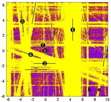
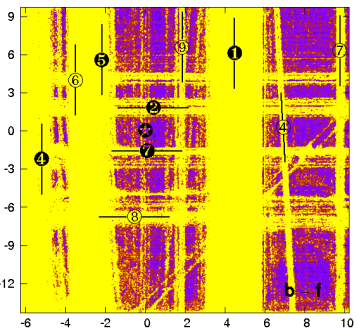
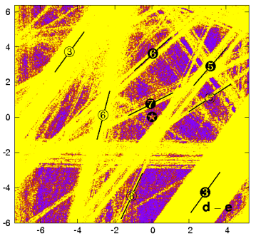
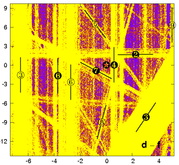
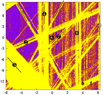
Let us now study the vicinity of these particular solutions through the dynamical maps. For each initial condition of the discrete grid with $512\times 512$ resolution, we compute $\langle Y\rangle$ over $T=8000$ yr. Figure 12 shows the MEGNO maps for solution IIa. Each panel is for a different pair of planets. The coordinate axes are rescaled mean motions centered at their nominal $n_{i,0}$:

$$x_{i}\equiv\frac{n_{i}-n_{i,0}}{n_{i,0}}\times 10^{4}.$$

The $x_{i}$–axes span $1\sigma$ uncertainties of the semi–major axes $a_{i}$, in accord with Tab. 2. The semi-major axes are determined very precisely, hence the $1\sigma$ interval span a range of $10^{-5}$ to $10^{-4}~{}\mbox{au}$. The rescaled $x_{i}$ are confined to order of $10$.

Figure 12: Symplectic MEGNO maps in the $(x_{i},x_{j})$–plane for solution IIa (see the text for details). Color scale for $\langle Y\rangle$ is $[1,5]$ (blue means $\langle Y\rangle\approx 2$ and stable solutions; yellow is for $\langle Y\rangle\gtrsim 5$ and unstable motions). Each panel is for different pair of planets labeled in its bottom-right corner.

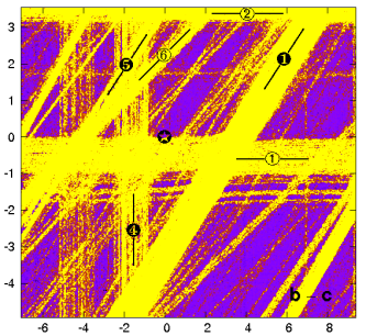
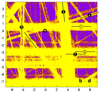
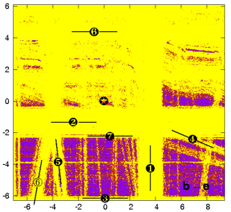
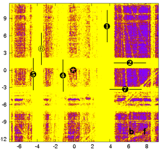
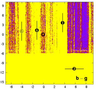
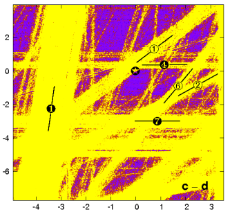
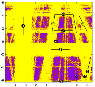
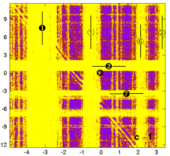
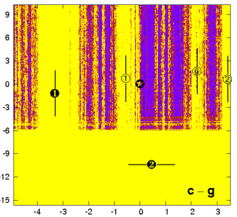
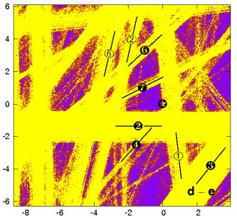
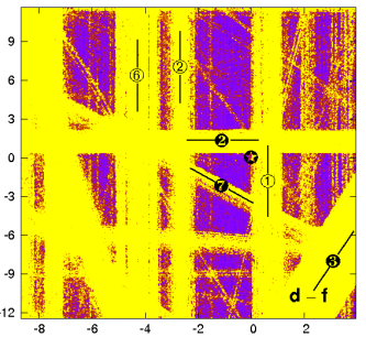
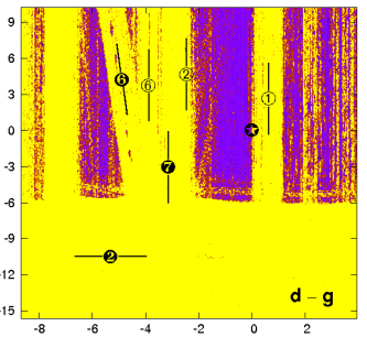
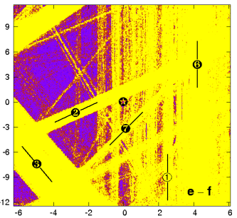
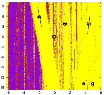
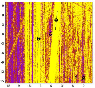
The MEGNO is color-coded in the dynamical maps. Blue regions mean regular solutions with $\langle Y\rangle\approx 2$, while yellow color is for chaotic (unstable) initial conditions, $\langle Y\rangle\geq 5$. The resolution is $512\times 512$ pixels, total integration time is $T=8000$ yr per pixel, SABA₄ integrator step-size is 0.5 days. A single computation of each map took $\sim 16$ hrs of 1200 CPU cores. The integrations of each pixel were performed up to the end time $T$, regardless a value of MEGNO.

Still, although the maps cover tiny regions of the phase space, close to the fixed initial condition, they reveal a sophisticated structure. Because we consider the dynamics in terms of conservative, close to integrable Hamiltonian system, this structure is governed by the resonant motions. A relatively short integration time $\sim 10^{4}$–$10^{5}$ characteristic periods, equivalent to the orbital period of the outermost planet makes it possible to detect unstable MMRs. They appear as yellow straight bands of different widths and slopes. Inspecting the dynamical maps, we can identify particular resonances.

A condition for the mean motion resonance in the $N$-planet system may be written in the following form:

$$\sum_{i=1}^{N}p_{i}{\frac{\mbox{d}\,\lambda_{i}}{\mbox{d\,}t}}=\mathcal{O}\left[f_{\omega},f_{\Omega}\right],\quad\mbox{or}\quad\sum_{i=1}^{N}p_{i}n_{i}=\mathcal{O}\left[f_{\omega},f_{\Omega}\right],$$ (3)

where $n_{i}$ is the mean motion of the $i$-th planet, $f_{\omega}$ and $f_{\Omega}$ are the fundamental frequencies associated with the pericenter arguments $\omega_{i}$ and the longitudes of nodes $\Omega_{i}$ (for all orbits), and $p_{i}$ are relatively prime integers. The linear relations must obey the d’Alambert rule.

The two-planet MMR takes place when two values of $p_{i}$ are non-zero. If three coefficients in this linear relation are non-zero, it means that the system exhibits 3–body MMR. In the Kepler-11 system, the fundamental frequencies associated with $\omega_{i}$ and $\Omega_{i}$ are much smaller than $n_{i}$ (these are the secular frequencies), hence the right-hand sides of Eq. 3 are close to $0$. This makes it possible to skip the secular terms, as the first order approximation, and to identify the MMRs through approximate resonance conditions involving the mean motions only.

To identify the MMRs in the MEGNO maps, we apply a simple method described in (Guzzo, 2005). In the $(n_{j},n_{k})$ –plane, the slope

$$\alpha_{j,k}\equiv\frac{\mbox{d}\,n_{k}}{\mbox{d}\,n_{j}}$$

of a particular resonance line determines the ratio of coefficients $p_{i}$, i.e.,

$$\alpha_{j,k}=-\frac{p_{j}}{p_{k}}.$$ (4)

If $\alpha_{j,k}=0$ then the MMR forms a horizontal line, planet $k$ is involved in the MMR, while planet $j$ is not. If $\alpha_{j,k}^{-1}=0$ then the MMR forms a vertical line, planet $j$ is involved in the resonance, while planet $k$ is not. In these cases, other planets may be involved in this particular resonance. If $\alpha_{j,k}$ is finite and non–zero then both considered planets are involved in the MMR. To identify this particular resonance, one has to compute slopes corresponding to this resonance in all $(n_{i},n_{j})$-planes. It may be not possible, if the map ranges do not cover the resonance band. If $\alpha_{j,k}$ is non-zero and finite only for one pair of planets ($j$, $k$), it means that 2–planet MMR is present. It should be verified whether $p_{j}n_{j}+p_{k}n_{k}\approx 0$. Coefficients $p_{j}$, $p_{k}$ of the MMR condition can be computed from the slopes $\alpha_{j,k}$. Similarly, the 3-body MMR takes place, if there exist relatively prime integers $i$, $j\neq i$ and $k\neq i,j$, such that $\alpha_{i,j},\alpha_{i,k}$ and $\alpha_{j,k}$ are all finite and non–zero. The 3-body MMR may be identified by computing the slope coefficients in appropriate planes of the mean motions. An identification of $4$–body and $N$–body MMRs can be derived as well.

Using this simple MMR identification algorithm, we found most significant MMRs close to solution IIa. The identified 3–body MMRs were labeled at the panels, and listed in Tab. 7. The mean motions of solution IIa permit a few low–order 2–body MMRs in the vicinity of this solution, e.g., $4n_{{\mbox{\scriptsize b}}}-5n_{{\mbox{\scriptsize c}}}$, $1n_{{\mbox{\scriptsize b}}}-3n_{{\mbox{\scriptsize e}}}$, $2n_{{\mbox{\scriptsize c}}}-5n_{{\mbox{\scriptsize e}}}$, $1n_{{\mbox{\scriptsize d}}}-2n_{{\mbox{\scriptsize f}}}$, $2n_{{\mbox{\scriptsize e}}}-3n_{{\mbox{\scriptsize f}}}$. There is no 2-planet MMR in the range of $n_{i}$ implied by $1\sigma$ uncertainty. All straight bands with finite and non-zero $\alpha_{i,j}$ have at least two images in the planes constructed for other planets. All features seen in the dynamical maps correspond then to $3$– and 4–body MMRs. Possibly, even more complex $N$-body resonances may be found.

Table 7: Three-planet resonances near the best–fit model IIa. See Fig. 12.

label	$p_{{\mbox{\scriptsize b}}}$	$p_{{\mbox{\scriptsize c}}}$	$p_{{\mbox{\scriptsize d}}}$	$p_{{\mbox{\scriptsize e}}}$	$p_{{\mbox{\scriptsize f}}}$	$p_{{\mbox{\scriptsize g}}}$
$1$	$7$	$-10$	$2$	$0$	$0$	$0$
$2$	$0$	$0$	$0$	$7$	$-11$	$2$
$3$	$0$	$0$	$5$	$-5$	$-3$	$0$
$4$	$1$	$0$	$-10$	$11$	$0$	$0$
$5$	$9$	$-13$	$0$	$4$	$0$	$0$
$6$	$0$	$0$	$6$	$-9$	$0$	$2$
$7$	$0$	$0$	$6$	$-16$	$11$	$0$
$1^{*}$	$0$	$5$	$-8$	$-1$	$0$	$0$
$2^{*}$	$0$	$6$	$-14$	$5$	$0$	$0$

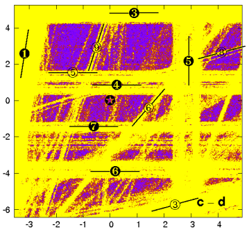
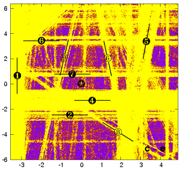
Labels in Fig. 12 corresponds to data in Tab. 7. Labels with asterisks are written in open circles in the dynamical maps and denote MMRs in the neighborhood of solution IIa. Resonances labeled with numbers without asterisks and written in filled circles in the dynamical map are also present in the neighbourhood of solution IIb.

The MMRs ($7n_{{\mbox{\scriptsize e}}}-11n_{{\mbox{\scriptsize f}}}+2n_{{\mbox{\scriptsize g}}}$) labeled as “2” and ($5n_{{\mbox{\scriptsize c}}}-8n_{{\mbox{\scriptsize d}}}-1n_{{\mbox{\scriptsize e}}}$) labeled as “$1^{*}$” are the most close to solution IIa. Solution IIa passed the $16000$ yr MEGNO test as stable solution. However, because it is close to two 3–body MMRs, and is found in a a dense web of low–order $3$–body and $4$-body MMRs, its long–term stability cannot be guaranteed by this test. The integration time of $16000$ yr corresponds to $\sim 50,000$ orbital periods of the outermost planet g. This time is usually too short to detect a chaotic nature of the orbit when the 3–body resonances are present. Unfortunately, the CPU-overhead does not permit to derive the dynamical map with the integration time per single initial condition which should be $10$–$10^{2}$–times longer. Indeed, a test run over $T=40,000$ yr illustrated in Fig. 13 reveals that solution IIa is chaotic and unstable. Besides, almost the whole $(x_{{\mbox{\scriptsize b}}},x_{{\mbox{\scriptsize c}}})$-plane corresponds to chaotic motions with $\langle Y\rangle>5$.

Figure 13: Dynamical map of solution IIa but for the integration time $40000$ yr per pixel. Mean motion resonances are labeled in accord with Table 7.

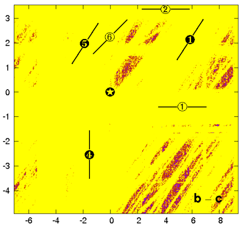
We analyzed the second solution IIb in the same manner. The MEGNO maps computed for $8000$ yr are presented in Fig. 14. Also these maps reveal a dense net of $3$-body and $4$-body resonances. Some of these resonances may be identified as close to solutions IIa as well as to IIb. They are labeled with the same numbers written within filled circles, as in Fig. 12. We found also a few new MMRs, labeled within open circles and labeled by “3”, “4” and “5”. The remaining 4–body MMRs which are visible in this figure are not labeled. All identified MMRs are listed in Tab. 8.

Figure 14: Symplectic MEGNO maps in the $(x_{i},x_{j})$–plane for solution IIb. Blue color means $\langle Y\rangle\approx 2$ (stable configuration), while yellow is for $\langle Y\rangle\gtrsim 5$ and unstable systems. Each panel is for different pair of planets labeled in the bottom-right corner of each particular panel. The resolution is $512\times 512$ pixels, total integration time is $8000$ yr per pixel, SABA₄ integrator step-size is 0.5 days.

Table 8: Three-planet resonances near solution IIb

label	$p_{{\mbox{\scriptsize b}}}$	$p_{{\mbox{\scriptsize c}}}$	$p_{{\mbox{\scriptsize d}}}$	$p_{{\mbox{\scriptsize e}}}$	$p_{{\mbox{\scriptsize f}}}$	$p_{{\mbox{\scriptsize g}}}$
$1$	$7$	$-10$	$2$	$0$	$0$	$0$
$2$	$0$	$0$	$0$	$7$	$-11$	$2$
$3$	$0$	$0$	$5$	$-5$	$-3$	$0$
$4$	$1$	$0$	$-10$	$11$	$0$	$0$
$5$	$9$	$-13$	$0$	$4$	$0$	$0$
$6$	$0$	$0$	$6$	$-9$	$0$	$2$
$7$	$0$	$0$	$6$	$-16$	$11$	$0$
$3^{*}$	$0$	$1$	$-6$	$6$	$0$	$0$
$4^{*}$	$13$	$-17$	$0$	$0$	$2$	$0$
$5^{*}$	$0$	$0$	$11$	$-21$	$8$	$0$

Similarly to configuration IIa, the integration over longer time of $T=40000$ yr, reveals that solution IIb is unstable. Almost the whole plane of the dynamical map corresponds to $\langle Y\rangle>5$. The MEGNO map is similar to Fig. 13, and is not shown here.

5.3 Dynamical maps in the $\boldsymbol{(\omega_{i},\omega_{j})}$– and $\boldsymbol{(e_{i},\Omega_{i})}$-planes.

Figure 15: Dynamical maps in the $(\omega_{i},\omega_{j})$–plane for solution IIa. The MEGNO range is $[1,5]$ and colour–coded: blue is for stable solutions, yellow is for unstable systems. Each map has elements of a given pair of planets varied, these planets are labeled in the bottom-right corner. The arguments of pericenter are expressed in degrees. The nominal solution is marked with the asterisk.

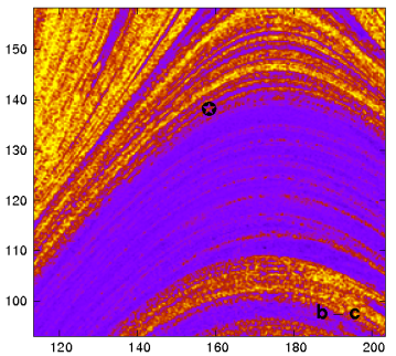
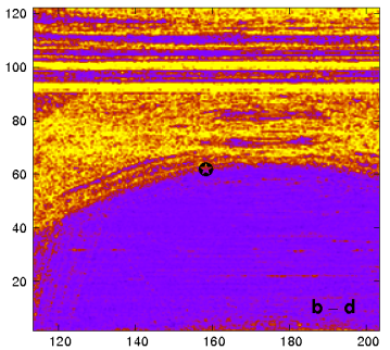
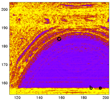
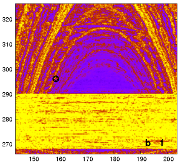
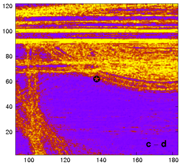
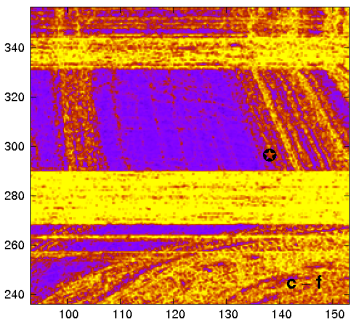
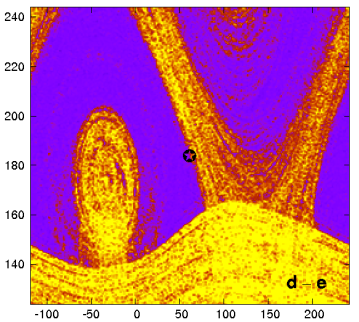
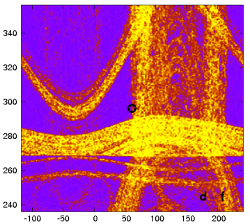
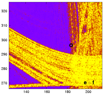
Figure 15 illustrates the MEGNO maps in planes of the arguments of pericenters. The MEGNO is calculated over $T=8000$ yr. The $(\omega_{i},\omega_{j})$–maps are constructed a bit differently than the mean motions dynamical maps. Because we intent to analyse configurations coherent with the observations, $\omega_{i}$ can be freely varied over the grid, if also the mean anomalies are modified to preserve the time of the first transit, $T_{i}$. For instance, for a circular orbit, when the argument of pericenter is shifted from the nominal value by $\Delta\omega_{i}$, the mean anomaly should be shifted by $-\Delta\omega_{i}$. For eccentric orbits such a correction flows from the Ist Keplerian law.

The MMRs form even more sophisticated web in the $(\omega_{i},\omega_{j})$–planes than in the mean motion planes. These dynamical maps reveal that the stability depends on the initial arguments of pericenters. It is not obvious a priori, because eccentricities are very small. The initial phases of the system are preserved across the maps, and each point corresponds to the same $T_{i}$. Keeping in mind that the photometric data spanning only $\sim 500$ days imply weak constraints on angles $\omega_{i}$, we realize how is difficult to find a stable initial conditions in the huge, $50$-dimensional parameter space of the system.

Figure 16: Dynamical maps in the $(e_{i},\Omega_{j})$-plane for solution IIa. The MEGNO range $[1,5]$ is colour coded: blue means stable solutions and yellow is for unstable configurations. Each map is constructed for a pair of planets labeled in the bottom-right corner. The longitudes of ascending nodes are expressed in degrees. The nominal solution is marked with an asterisk. See Tab. 5 for the orbital elements of this best–fit model.

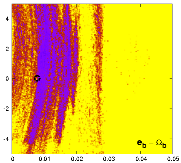
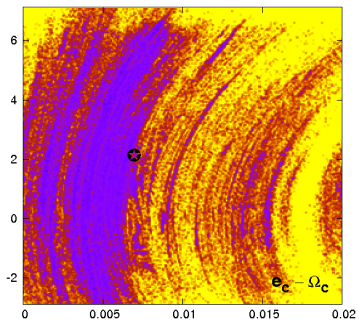
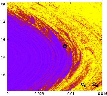
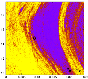
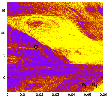
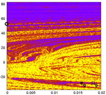
Figure 16 illustrates MEGNO maps in the $(e_{i},\Omega_{i})$ -planes calculated over $T=8000$ yr. Each panel is for one planet. An identification of particular MMRs is much more complex than in the mean motion planes. It would require the frequency analysis of these solutions. Still, regions of stable, quasi-periodic motions usually form only small islands in the phase space. For the four innermost planets, the regular motions are confined to only $\sim 5^{\circ}$ range of $\Omega_{i}$ around the nominal value and also to a small range of eccentricities $\sim 0.01$. For the two outermost planets f and planet g the maps look like different. A zone of stable motions of planet g extends towards large $\Omega_{g}$. It implies a large mutual inclination of its orbit to the rest of the system. Small $\Omega_{g}$ provoke unstable motions. The nominal solution is found at the very edge between the regular and chaotic zone.

5.4 Stable solution of model IV

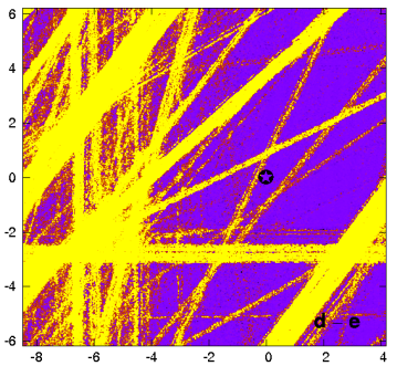
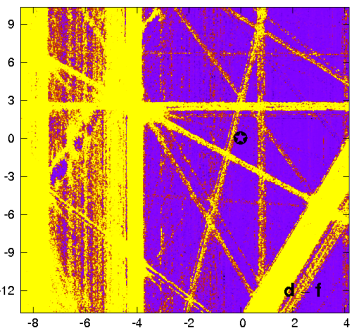
Let us recall that in transit model IV all $\Omega_{i}=0^{\circ}$. Hence, the mutual inclinations between all pairs of orbits are close to $0^{\circ}$ but the system remains non-coplanar because $I_{i}$ is still different from $90^{\circ}$ (hence, the transits of all planets in this system can be detected by a randomly located observer with a significant probability of $\sim 3.4\%$). In this case we found several solutions with MEGNO converging to $2$ after $T=16000$ yr. This indicates a possibility of quasi-regular orbits. We chose one of such solutions. Its parameters are listed in Tab. 9, and we compute dynamical maps in its vicinity. Figure 17 shows the results of this experiment in the mean motions planes. The integration time is $T=8000$ yr per pixel.

Table 9: Orbital parameters of solution IVa. Mass of the star is $0.95\,\mbox{m}_{\sun}$. Osculating elements of Poincaré are given at the epoch JD 2455964.51128.

parameter/planet	b	c	d	e	f	g
$m\,[\mbox{m}_{\earth}]$	$2.359$	$3.386$	$5.630$	$10.841$	$7.524$	$25.161$
$a\,[\mbox{au}]$	$0.091113$	$0.106505$	$0.154243$	$0.193940$	$0.249511$	$0.463991$
$e$	$0.04423$	$0.01719$	$0.00633$	$0.00258$	$0.01073$	$0$ (fixed)
$I\,$ [deg]	$89.141$	$91.215$	$89.332$	$88.837$	$89.394$	$89.770$
$\omega\,$ [deg]	$20.651$	$55.728$	$140.753$	$236.761$	$355.845$	$0$ (fixed)
$\mathcal{M}\,$ [deg]	$178.88174$	$209.60077$	$40.79259$	$318.51831$	$91.57569$	$336.26502$

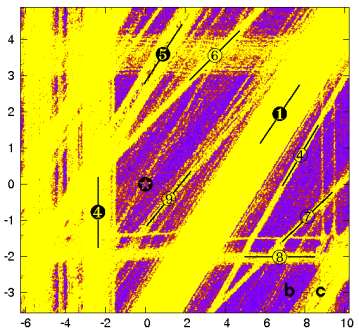
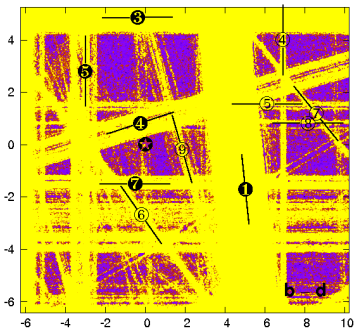
The tested configurations is found in a narrow region of regular motions. The most prominent dynamical feature visible in the maps is associated with stable 3-planet MMR between planets b, c and d. We identified it as $(7,-10,2,0,0,0)$ MMR. It has been also found in dynamical maps associated with solutions IIa and IIb as the MMR labeled as “1”. Due to altered parameters of the model, the unstable region of this resonance is visible in these maps. The solid black lines plotted across panels shown in the top row of Fig. 17 have the slope equal to ${7}/{10}$, $-{7}/{2}$ and $5$, from the left to the right, respectively. Other 3-body resonances visible in the dynamical maps form a dense web, which may be better seen in the $(x_{{\mbox{\scriptsize d}}},x_{{\mbox{\scriptsize e}}})$– and $(x_{{\mbox{\scriptsize d}}},x_{{\mbox{\scriptsize f}}})$–planes displayed in the bottom panels.

Figure 17: Dynamical maps of solution IVa in the mean motions planes. The colours and symbols are the same as in Fig. 12.

Figure 18: Dynamical map of solution IVa in the mean motion plane of planet b and planet c but for longer integration time of $T=40,000$ yr. See Fig. 17 for an explanation of the symbols and colour coding.

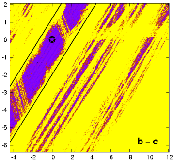
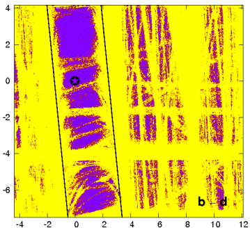
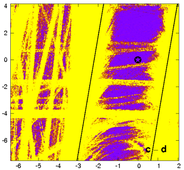
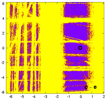
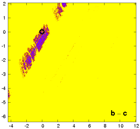
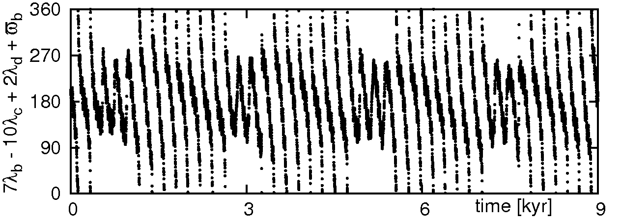
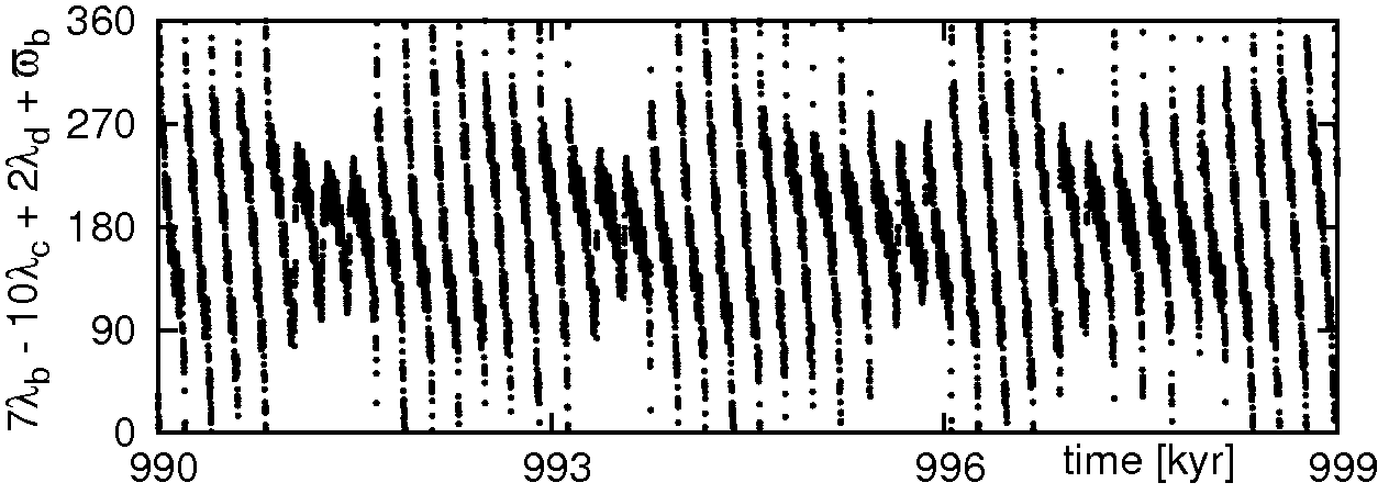
To examine the stability of this solution over longer time scale, we calculated a single dynamical map in the $(x_{{\mbox{\scriptsize b}}},x_{{\mbox{\scriptsize c}}})$ –plane for much longer integration time $T=40000$ yr. It is shown in Fig. 18. This solution is located in a tiny region of stable motions. In this case, the 3–body MMRs has a protective role for the system, saving it from a disruption. Actually, this solution is chaotic. To demonstrate this, we computed the critical argument of the 3–body MMR and we plot over two intervals of time, at the beginning of the 1 Myr integration period (the left panel of Fig. 19) and at the end of this period (the right panel of Fig. 19). The critical arguments exhibit librations alternated with circulations. Such behavior of the critical argument indicates a crossing of the separatrix of the resonance, and chaotic dynamics. In such a case, the configuration may be geometrically stable over very long time but it may be suddenly disrupted due to a slow diffusion along the resonance.

Figure 19: Temporal evolution of the critical argument of the 3-body MMR for the initial condition IVa. The left panel is for the beginning of the integration period, and the right panel is for the end of the integration period spanning 1 Myr.

5.5 The Arnold web structure in the phase space

The results of experiments described in the previous sections may be interpreted at the ground of the dynamical systems theory. The dynamical stability of planetary orbits in systems with strong perturbations is influenced by even small errors and the resulting diffusion due to resonances overlapping. This dynamical phenomenon has been investigated in the Outer Solar system. Murray & Holman (2001) identified the chaos among the Jovian planets as resulting from the overlap of the components of 3–body MMRs among Jupiter, Saturn, and Uranus. In spite of short Lyapunov time ($10^{7}$ years), they found the dynamical lifetime of Uranus $\sim 10^{18}$ years. In this way, the analytic theory of Murray & Holman (2001) explained an apparent paradox of long–term stable system which is actually chaotic.

The structure of the 3–body and 4–body MMRs in the Outer Solar system was further investigated numerically by Guzzo (2005, 2006). Very recently, it was also studied by Quillen (2011) for strongly interacting extrasolar systems. Through the dynamical maps technique, Guzzo (2005) found that if the chaotic motions appear in a regular net, they may be practically stable over very long times. Such a state of chaotic system is called the Nekhoroshev regime. On contrary, if the chaotic resonances do not constitute a regular web, and minority of orbits form a global chaotic zone, the stability of the system is influenced by strong chaotic diffusion. Such regime is related to the resonance overlap, and is called the Chirikov regime of the dynamics (Froeschlé et al., 2000; Guzzo, 2005).

These results may be applied to interpret the dynamical maps of the Kepler-11 system. The dense net of the multiple-body MMRs form the Arnold web in the neighborhood of the best fit model configurations. Our experiments reveal, that this system may undergo the Chirikov regime rather than long-term stable Nekhoroshev regime. We have no strong proof of this phenomenon, because it would require non-trivial and intensive computations of the chaotic diffusion. Conclusions regarding the real state of the Kepler-11 system require more precise determination of the initial conditions than obtained in this work.

We also note that solutions IIa, IIb investigated in detail are found at the very border of the chaotic and regular zones. This can be well seen in the ${(\omega_{i},\omega_{j})}$– and ${(e_{i},\Omega_{i})}$-planes. A change of these angles constrained by the best–fit errors, could “move” the system into larger zones of stable motions. Because the MEGNO quantifies the stability of the system as a whole, such a change would imply a shift of the initial condition in all parameter maps (Goździewski & Maciejewski, 2001). The altered initial conditions would be also more “distant” from the unstable strips of 3–body and 4–body MMRs in the mean motions planes. The dynamical maps would be more similar to those computed for solution IV revealing most extended zones of stable motions. Overall, the dynamical state of the system is very fragile and depends on subtle changes of the initial conditions.

Still most of the best-fit model configurations obtained with the bootstrap algorithm, which appear as regular over the short-term dynamics time–scale are self–disrupting. This behavior is similar to unstable evolution in 3–body MMRs observed in the HD 37124 system (Goździewski et al., 2008). In this sense the dynamical state of the Kepler-11 system is still puzzling. The results of long–term integrations of the obtained sets of initial conditions indicate that the system resides at the edge of dynamical stability. These conclusions might be changed, if more data are gathered and analyzed.

6 Conclusions

In this paper, we derived an improved method for the dynamical analysis of photometric light curves of stars with multiple transiting planets. Its main purpose is to determine planetary masses, as well as a number of indirect parameters affecting the dynamical stability of the system. This algorithm improved the well known TTV algorithm. The crucial point of this method is to model the whole photometric curve directly with the help of an efficient symplectic $N$-body integration. Such the direct approach make is possible to account for multiple transits, as well for the transit depths and their widths. This in turn makes it possible to impose dynamical constraints on parameters which cannot be determined in terms of the TTV, like the longitude of nodes and mutual inclinations of orbits.

With the help of this new method, we re-analyzed available photometric data for Kepler-11. The direct algorithm imposes constraints on the mass of the outermost planet g and help us to determine the mutual inclinations between orbits of planets b and planet c as well as between the (d-e) pair with a good accuracy of $2^{\circ}$. These results extend analysis performed in the discovery paper (Lissauer et al., 2011). Overall, conclusions in this paper and in our work coincide very well, in spite of quite a different transit models, optimisation algorithms and uncertainties estimation methods applied.

Thanks to the in–depth analysis of the Kepler-11 light-curves, we investigated a possible chemical composition of the planets detected in this intriguing system. The most curious finding is a clear anti-correlation of the mean densities of the planets with their mean distances from the star. The inner planets exhibit larger abundance of heavy elements than the outer companions. Because all eccentricities as well as the mutual inclinations of stable systems remains small, the system unlikely suffered violent scattering processes in the past. It follows that the ordering of planets have been preserved since their formation. A dynamical relaxation should imply large $e_{i}$ and $\Delta I_{i,j}$ (see, e.g., Chatterjee et al., 2008; Adams & Laughlin, 2003). These factors indicate that the primordial protoplanetary disk might have a significant gradient of metallicity and the present Kepler-11 system is a real fossil of this disk. If this suggestion is confirmed, it can constrain the planet formation theories, in particular concerning multiple systems of super–Earth planets.

This conclusion is reinforced by the dynamical analysis of the system. We found, in accord with the discovery paper, that the system is basically free from 2-planet MMRs. However, its global dynamics is governed by $3$-body and $4$–body MMRs. Overlapping of these resonances near the best-fit solutions imply an extended zone of dynamical chaos and very unstable configurations. Particular multi-body resonances may stabilize the system. We identified such a 3–body resonance. However, the observation window spanning only $\sim 500$ days does not make it possible to pick up this MMR as the only possible. Besides, the MMRs form the structure of the Arnold web characteristic for the Chirikov regime. In this dynamical state, the phase-space orbits are strongly unstable due to overlapping of the MMRs. In such a case, the chaotic diffusion in the actions (semi–major axes) space is significant and easily leads to strong geometric changes of orbits. Actually, our numerical experiments indicate this in the Kepler-11 system. It remains an open question though, how such an apparently ordered configuration of planets could survive the formation phase in extremely complex and fragile dynamical environment.

The discovery team argue that the system is non-resonant. This factor would prevent a scenario of trapping the planets into MMRs during the inward migration at the early stages of the evolution. As we showed here, the system is in fact extremely resonant, but in quite a different sense. Combining this fact with small values of the eccentricities and anti–correlation of the chemical composition with the distance to the star, we may conclude quite an opposite: the migration/trapping scenario could be the only way of preserving the primary architecture in the present form. However, these suggestions might be verified only if more photometric data are gathered and are available.

Most likely, many other Kepler–discovered multiple extrasolar systems with transiting planets exhibit qualitatively similar behaviours to that one we found in the Kepler-11. Hence, the approach in this paper is general and may be applied in the studies of other compact systems composed of low-massive, super–Earth or Neptune-like planets.

References

- Adams & Laughlin (2003) Adams F. C., Laughlin G., 2003, Icarus, 163, 290
- Agol et al. (2005) Agol E., Steffen J., Sari R., Clarkson W., 2005, MNRAS, 359, 567
- Baluev (2009) Baluev R. V., 2009, MNRAS, 393, 969
- Barnes et al. (2008) Barnes R., Goździewski K., Raymond S. N., 2008, ApJL, 680, L57
- Batalha et al. (2011) Batalha N. M., Borucki W. J., Bryson S. T., Buchhave L. A., Caldwell D. A., Christensen-Dalsgaard J., Ciardi D., Dunham E. W., Fressin F., Gautier III T. N., Gilliland R. L., Haas M. R., Howell S. B., Jenkins J. M., Kjeldsen H., Koch D. G., 2011, ApJ, 729, 27
- Batalha et al. (2012) Batalha et al. N. M., 2012, ArXiv 1202.5852
- Borucki et al. (2010) Borucki W. J., Koch D., Basri G., Batalha N., Brown T., Caldwell D., Caldwell J., Christensen-Dalsgaard J., Cochran W. D., DeVore E., Dunham E. W., 2010, Science, 327, 977
- Borucki et al. (2011) Borucki et al. W. J., 2011, ApJ, 736, 19
- Caldwell et al. (2010) Caldwell D. A., Kolodziejczak J. J., Van Cleve J. E., Jenkins J. M., Gazis P. R., Argabright V. S., Bachtell E. E., Dunham E. W., Geary J. C., Gilliland R. L., Chandrasekaran H., Li J., 2010, ApJL, 713, L92
- Carter et al. (2012) Carter J. A., Agol E., Chaplin W. J., Basu S., Bedding T. R., Buchhave L. A., Christensen-Dalsgaard J., Deck K. M., Elsworth Y., Fabrycky D. C., Ford E. B., Fortney J. J., Hale S. J., Handberg R., Hekker S., Holman M. J., Huber D., 2012, ArXiv e-prints
- Carter et al. (2011) Carter J. A., Fabrycky D. C., Ragozzine D., Holman M. J., Quinn S. N., Latham D. W., Buchhave L. A., Van Cleve J., Cochran W. D., Cote M. T., Endl M., Ford E. B., Haas M. R., Jenkins J. M., 2011, Science, 331, 562
- Charbonneau (1995) Charbonneau P., 1995, ApJS, 101, 309
- Chatterjee et al. (2008) Chatterjee S., Ford E. B., Matsumura S., Rasio F. A., 2008, ApJ, 686, 580
- Cincotta et al. (2003) Cincotta P. M., Giordano C. M., Simó C., 2003, Physica D Nonlinear Phenomena, 182, 151
- Cincotta & Simó (2000) Cincotta P. M., Simó C., 2000, A&A Supl., 147, 205
- Cochran et al. (2011) Cochran W. D., Fabrycky D. C., Torres G., Fressin F., Désert J.-M., Ragozzine D., Sasselov D., Fortney J. J., Rowe J. F., Brugamyer E. J., Bryson S. T., Carter J. A., Ciardi D. R. e. a., 2011, ApJS, 197, 7
- Deb (2004) Deb K., 2004, IPSJ Transactions on Mathematical Modeling and Its Applications, 45, 1
- Fabrycky et al. (2012) Fabrycky D. C., Ford E. B., Steffen J. H., Rowe J. F., Carter J. A., Moorhead A. V., Batalha N. M., Borucki W. J., Bryson S., Buchhave L. A., Christiansen J. L., Ciardi D. R., Cochran e. a., 2012, ArXiv e-prints
- Ford et al. (2012) Ford E. B., Fabrycky D. C., Steffen J. H., Carter J. A., Fressin F., Holman M. J., Lissauer J. J., Moorhead A. V., Morehead R. C., Ragozzine D., Rowe J. F., Welsh W. F., Allen C., Batalha N. M., Borucki W. J., Bryson S. T., Buchhave L. A. e. a., 2012, ArXiv e-prints
- Fressin et al. (2011) Fressin F., Torres G., Désert J.-M., Charbonneau D., Batalha N. M., Fortney J. J., Rowe J. F., Allen C., Borucki W. J., Brown T. M., Bryson S. T., Ciardi D. R., Cochran W. D., Deming D., Dunham E. W., Fabrycky D. C., Gautier III T. N., Gilliland R. L., 2011, ApJS, 197, 5
- Fressin et al. (2011) Fressin F., Torres G., Rowe J. F., Charbonneau D., Rogers L. A., Ballard S., Batalha N. M., Borucki W. J., Bryson S. T., Buchhave L. A., Ciardi D. R., Desert J.-M., Dressing C. D., Fabrycky D. C., 2011, ArXiv e-prints
- Froeschlé et al. (2000) Froeschlé C., Guzzo M., Lega E., 2000, Science, 289, 2108
- Gautier et al. (2011) Gautier III T. N., Charbonneau D., Rowe J. F., Marcy G. W., Isaacson H., Torres G., Fressin F., Rogers L. A., Désert J.-M., Buchhave L. A., Latham D. W., Quinn S. N., Ciardi D. R., Fabrycky D. C., Ford E. B., Gilliland R. L., Walkowicz L. M., 2011, ArXiv e-prints
- Goździewski (2003) Goździewski K., 2003, A&A, 398, 315
- Goździewski et al. (2008) Goździewski K., Breiter S., Borczyk W., 2008, MNRAS, 383, 989
- Goździewski & Maciejewski (2001) Goździewski K., Maciejewski A. J., 2001, ApJL, 563, L81
- Goździewski et al. (2008) Goździewski K., Migaszewski C., Musieliński A., 2008, in Y.-S. Sun, S. Ferraz-Mello, & J.-L. Zhou ed., IAU Symposium Vol. 249 of IAU Symposium, Stability constraints in modeling of multi-planet extrasolar systems. pp 447–460
- Guillot (1999) Guillot T., 1999, Science, 296, 72
- Guzzo (2005) Guzzo M., 2005, Icarus, 174, 273
- Guzzo (2006) Guzzo M., 2006, Icarus, 181, 475
- Helled et al. (2011) Helled R., Anderson J. D., Podolak M., Schubert G., 2011, ApJ, 726, 15
- Holman et al. (2010) Holman M. J., Fabrycky D. C., Ragozzine D., Ford E. B., Steffen J. H., Welsh W. F., Lissauer J. J., Latham D. W., Marcy G. W., Walkowicz L. M., Batalha N. M., Jenkins J. M., Rowe J. F., Cochran W. D., Fressin F., Torres G., 2010, Science, 330, 51
- Holman & Murray (2005) Holman M. J., Murray N. W., 2005, Science, 307, 1288
- Howarth (2011) Howarth I. D., 2011, MNRAS, 418, 1165
- Jenkins et al. (2010) Jenkins J. M., Caldwell D. A., Chandrasekaran H., Twicken J. D., Bryson S. T., Quintana E. V., Clarke B. D., Li J., Allen C., Tenenbaum P., Wu H., Klaus T. C., Middour C. K., Cote M. T., McCauliff S., Girouard F. R., 2010, ApJL, 713, L87
- Koch et al. (2010) Koch D. G., Borucki W. J., Basri G., Batalha N. M., Brown T. M., Caldwell D., Christensen-Dalsgaard J., Cochran W. D., DeVore E., Dunham E. W., Gautier III T. N., Geary J. C., Gilliland R. L., Gould A., Jenkins J., 2010, ApJL, 713, L79
- Laskar & Robutel (2001) Laskar J., Robutel P., 2001, Celestial Mechanics and Dynamical Astronomy, 80, 39
- Lissauer et al. (2011) Lissauer J. J., Fabrycky D. C., Ford E. B., Borucki W. J., Fressin F., Marcy G. W., Orosz J. A., Rowe J. F. ., 2011, Nature, 470, 53
- Lissauer et al. (2012) Lissauer J. J., Marcy G. W., Rowe J. F., Bryson S. T., Adams E., Buchhave L. A., Ciardi D. R., Cochran W. D., Fabrycky D. C., Ford E. B., Fressin F., Geary J., Gilliland R. L., Holman M. J., Howell S. B. e. a., 2012, ArXiv e-prints
- Lynden-Bell & O’Dwyer (2001) Lynden-Bell D., O’Dwyer J. P., 2001, ArXiv Astrophysics e-prints
- Lynden-Bell & Tout (2001) Lynden-Bell D., Tout C. A., 2001, ApJ, 558, 1
- Mandel & Agol (2002) Mandel K., Agol E., 2002, ApJ, 580, L171
- Mikkola & Innanen (1999) Mikkola S., Innanen K., 1999, Celestial Mechanics and Dynamical Astronomy, 74, 59
- Morbidelli (2002) Morbidelli A., 2002, Modern celestial mechanics : aspects of solar system dynamics
- Murray & Holman (2001) Murray N., Holman M., 2001, Nature, 410, 773
- Nesvorný et al. (2012) Nesvorný D., Kipping D. M., Buchhave L. A., Bakos G. Á., Hartman J., Schmitt A. R., 2012, Science, 336, 1133
- Pál (2011) Pál A., 2011, MNRAS, p. 2123
- Press et al. (1992) Press W. H., Teukolsky S. A., Vetterling W. T., Flannery B. P., 1992, Numerical recipes in C. The art of scientific computing
- Quillen (2011) Quillen A. C., 2011, MNRAS, 418, 1043
- Rogers et al. (2011) Rogers L. A., Bodenheimer P., Lissauer J. J., Seager S., 2011, ApJ, 738, 59
- Slonina et al. (2012) Slonina M., Gozdziewski K., Migaszewski C., 2012, ArXiv e-prints
- Steffen et al. (2012) Steffen J. H., Fabrycky D. C., Ford E. B., Carter J. A., Désert J.-M., Fressin F., Holman M. J., Lissauer J. J., Moorhead A. V., Rowe J. F., Ragozzine D., Welsh W. F., Batalha N. M., Borucki W. J., Buchhave L. A., Bryson S. e. a., 2012, MNRAS, 421, 2342
- Wisdom & Holman (1991) Wisdom J., Holman M., 1991, AJ, 102, 1528