Likelihood, Fisher information, and systematics of cosmic microwave background experiments

Every experiment is affected by systematic effects that hamper the data analysis and have the potential to ultimately degrade its performance. In the case of probes of the cosmic microwave background (CMB) radiation, a minimal set of issues to consider includes asymmetric beam functions, correlated noise, and incomplete sky coverage. Presuming a simplified scanning strategy that allows for an exact analytical treatment of the problem, we study the impact of systematic effects on the likelihood function of the CMB power spectrum. We use the Fisher matrix, a measure of the information content of a data set, for a quantitative comparison of different experimental configurations. In addition, for various power spectrum coefficients, we explore the functional form of the likelihood directly, and obtain the following results: The likelihood function can deviate systematically from a Gaussian distribution up to the highest multipole values considered in our analysis. Treated exactly, realistic levels of asymmetric beam functions and correlated noise do not by themselves decrease the information yield of CMB experiments nor do they induce noticeable coupling between multipoles. Masking large fractions of the sky, on the other hand, results in a considerably more complex correlation structure of the likelihood function. Combining adjacent power spectrum coefficients into bins can partially mitigate these problems.

1 Introduction

Owing to its sensitive shape dependence on the most fundamental cosmological parameters, the power spectrum of the cosmic microwave background (CMB) radiation is one of the most important probes of the properties of the early universe (Mukhanov 2004). As a consequence, a large number of experiments have been designed to improve the observational constraints on the CMB anisotropies (e.g., Smoot et al. 1992; Netterfield et al. 2002; Bennett et al. 2003; Kuo et al. 2004; Dunkley et al. 2011; Keisler et al. 2011; Planck Collaboration et al. 2011). With the increasing precision of observations, the demands on the numerical tools used for data analysis became more and more stringent. Given the data obtained with the Planck satellite, for example, the temperature power spectrum will be cosmic variance limited from the largest scales up to a multipole moment of about $\ell\approx 2500$ (Efstathiou et al. 2005). To take full advantage of this wealth of information, a precise understanding and thorough modeling of the data properties are necessary.

The Fisher information matrix is ubiquitous in statistics. Used in the context of the Cramer-Rao bound, it permits a quantitative assessment of an experiment’s ability to constrain a set of parameters. Furthermore, it also allows drawing conclusions about parameter degeneracies. Owing to its predictive power, the Fisher matrix has been widely used to characterize and optimize experiments in various fields of astronomy (for example, in cosmology, e.g., Hu & Tegmark 1999; Berti et al. 2005; Rimes & Hamilton 2005; Lee & Pen 2008). Since the computational costs associated with its numerical calculation are prohibitively large, such studies have not been realized for general high-resolution CMB experiments. Elsner & Wandelt (2012) introduced a method for an efficient yet exact calculation of the Fisher matrix and of the full likelihood in only ${{\cal O}\!\left(\ell_{\mathrm{max}}^{4}\right)}$ operations. This mathematical framework enables a quantitative study of several systematic effects on CMB power spectrum constraints. In this work, we focus on common systematics like asymmetric beam functions, correlated noise, partial sky coverage, and the effect of binning. For different experimental setups, we analyze the correlation structure of the power spectrum coefficients and explore the shape of the likelihood function itself.

Cosmological parameter estimation from a power spectrum is commonly performed by means of Monte Carlo sampling techniques (e.g. Christensen & Meyer 2000; Lewis & Bridle 2002). Owing to the costs associated with the numerical evaluation of the full likelihood function given the data map, exact methods are restricted to the lowest multipole moments, $\ell_{\mathrm{max}}\la 50$ (e.g. Hinshaw et al. 2007; Gruppuso et al. 2009). Beyond that, the likelihood function is usually written in terms of the power spectrum coefficients themselves, a considerably less demanding problem. To do so, the function has to be approximated by, e.g., a multivariate Gaussian distribution (as done for the analysis of the Atacama Cosmology Telescope data, Dunkley et al. 2011), or some other choice, such as a combination of a Gaussian and an offset log-normal distribution (as done by the WMAP team, Verde et al. 2003). Using our methods, we are able to give examples of generic features of the true underlying likelihood function which should be reproduced by these approximations to avoid introducing systematic biases in the cosmological parameter determinations.

Since our method allows an exact modeling of the data in its full complexity, we can address a new question about how different instrumental and experimental properties affect the information content of a CMB data set: rather than asking how systematics affect results if they are not taken into account optimally (see, e.g., the discussion of correlated noise in Delabrouille 1998; Maino et al. 1999, asymmetric beams in Burigana & Sáez 2003; Mitra et al. 2011, and partial sky coverage in Szapudi et al. 2001; Wandelt et al. 2001; Hivon et al. 2002), we can determine to what extent these systematics fundamentally degrade power spectrum constraints even after an analysis that takes their effects into account optimally. In all the analyses we present in this paper, the instrumental characteristics of the simulated experiment (such as the noise model and the asymmetric beam maps) are assumed to be known exactly. To make this assumption true for realistic experiments requires a careful calibration strategy. Therefore, the results we discuss should be seen as hard lower limits on the effects of systematics on CMB power spectrum inferences.

The paper is organized as follows. In Sect. 2, we briefly review the mathematical background used for our study. We then assess the impact of important experimental systematics on the likelihood function (Sect. 3). Finally, we summarize our findings in Sect. 4.

2 The likelihood analysis on the ring torus

Consider an arbitrary CMB experiment with Gaussian noise, the likelihood function ${\cal L}$ of the data $d$ is

$${\cal L}(C_{\ell}|d)=\frac{1}{\sqrt{|2\pi(\mathbf{S}(C_{\ell})+\mathbf{N})|}}\\ \times\exp\left[{-\frac{1}{2}\,d^{\dagger}(\mathbf{S}(C_{\ell})+\mathbf{N})^{-1}d}\right]\,,$$ (1)

where we have introduced the signal covariance matrix, $\mathbf{S}$, as a function of the CMB power spectrum coefficients $C_{\ell}$. The noise properties are characterized by the noise covariance matrix, $\mathbf{N}$.

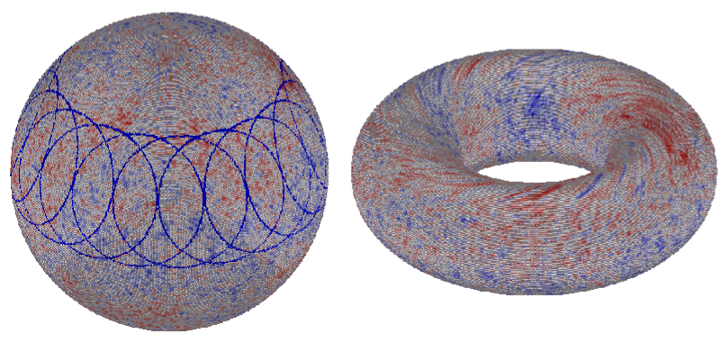
In the most general case, the evaluation of Eq. (1) takes ${{\cal O}\!\left(N^{3}\right)}$ operations, where $N$ is the number of pixels in the survey (Borrill 1999). To enable a numerically feasible analysis, we only consider experiments with an idealized scanning strategy, where the sky is observed on iso-latitude circles. The mathematical background of the algorithm is explained in detail in Wandelt & Hansen (2003) and Elsner & Wandelt (2012). Following their approach, we then map the time-ordered data (TOD) onto the ring torus. We visualize this duality in Fig. 1. Casting the equations into Fourier space allows us to take advantage of the periodicity of the manifold – the expression for the likelihood function simplifies.

Figure 1: Idealizing the scanning strategy leads to additional symmetries. Observing the sky on iso-latitude rings with a regular spacing in azimuthal direction (left panel) allows to map the resulting data structure onto a ring torus (right panel). Then, the formulation of the likelihood function in Fourier basis simplifies.

To obtain the signal covariance matrix in Fourier basis, we specify the noise-free sky temperature as a function of the spherical harmonic coefficients of a signal map, $a_{\ell m}$,

$$T^{S}_{rp}=\sum_{\ell}a_{\ell r}\,d^{\ell}_{rp}(\theta_{\mathrm{s}})\,X_{\ell p}\,.$$ (2)

Here, the index $p$ specifies the Fourier modes in the in-ring direction, and $r$ labels the index for the cross-ring direction. In Eq. (2), we make use of the definition of the Wigner rotation matrix to introduce the real quantity $d$,

$$D^{\ell}_{mm^{\prime}}(\phi_{2},\theta,\phi_{1})=\mathrm{e}^{-\mathrm{i}m\phi_{2}}\,d^{\ell}_{mm^{\prime}}(\theta)\,\mathrm{e}^{-\mathrm{i}m^{\prime}\phi_{1}}\,,$$ (3)

which we evaluate at the latitude of the experiment’s spin axis, $\theta=\theta_{\mathrm{s}}$. We also apply the rotated beam $X$ according to

$$X_{\ell m}=\sqrt{\frac{2\ell+1}{4\pi}}\sum_{m^{\prime}}d^{\ell}_{mm^{\prime}}(\theta_{\mathrm{o}})\,b_{\ell m^{\prime}}^{\ast}\,,$$ (4)

where the Wigner small $d$ matrix is now computed at the opening angle of the scanning circles, $\theta_{\mathrm{o}}$. The spherical harmonic expansion coefficients of the beam pattern, $b_{\ell m}$, are taken into account exactly and need not to be azimuthally averaged. The signal covariance matrix $\langle T^{S}_{rp}T^{S\,\ast}_{r^{\prime}p^{\prime}}\rangle$ then simplifies,

$$\mathbf{S}_{rpr^{\prime}p^{\prime}}=\delta_{rr^{\prime}}N^{2}\sum_{\ell}C_{\ell}\,d^{\ell}_{rp}X_{\ell p}\,d^{\ell}_{r^{\prime}p^{\prime}}X_{\ell p^{\prime}}^{\ast}\,.$$ (5)

In Fourier space, $\mathbf{S}$ shows a block diagonal structure.

We now specify the noise correlations. For an experiment with stationary noise, we can fully characterize its properties by a power spectrum $P(k)$ in the TOD domain. This ansatz is general enough to include the exact treatment of, e.g., $1/f^{2}$-type noise, a common systematic in real-world experiments. The noise covariance matrix $\langle T^{N}_{rp}T^{N\,\ast}_{r^{\prime}p^{\prime}}\rangle$ now reduces to

$$\mathbf{N}_{rpr^{\prime}p^{\prime}}=\delta_{rr^{\prime}}\frac{1}{N_{\mathrm{r}}N_{\mathrm{p}}^{2}}\sum_{m,m^{\prime}=0}^{N_{\mathrm{p}}-1}\mathrm{e}^{-\frac{2\pi\mathrm{i}}{N_{\mathrm{p}}}(pm-p^{\prime}m^{\prime})}\\ \times\sum_{\Delta=0}^{N_{\mathrm{r}}-1}\mathrm{e}^{-\frac{2\pi\mathrm{i}}{N_{\mathrm{r}}}\Delta r}C(\Delta,m,m^{\prime})\,,$$ (6)

where $N_{\mathrm{p}}$ is the number of pixels per ring, and $N_{\mathrm{r}}$ is the number of rings in the data set. We introduced an auxiliary function $C(\Delta,m,m^{\prime})$ according to

$$C(\Delta,m,m^{\prime})=\sum_{k=0}^{N-1}P(k)\,e^{-\frac{2\pi\mathrm{i}}{N}k(N_{\mathrm{r}}\Delta+m-m^{\prime})}\,.$$ (7)

In a Fourier space representation, we also find the noise covariance matrix $\mathbf{N}$ to be block diagonal.

We now review an efficient scheme to calculate the Fisher information matrix. Defined as the covariance of the score function, from Eq. (1), we obtain (Tegmark 1997)

$$F_{\ell_{1}\ell_{2}} =-\left\langle\frac{\partial^{2}\ln{\cal L}}{\partial C_{\ell_{1}}\partial C_{\ell_{2}}}\right\rangle$$

$$=\frac{1}{2}\,\mathrm{tr}\left[\mathbf{C}^{-1}\mathbf{P}^{\ell_{1}}\mathbf{C}^{-1}\mathbf{P}^{\ell_{2}}\right]\,,$$ (8)

where $\mathbf{C}=\mathbf{S}+\mathbf{N}$, and $\mathbf{P}^{\ell}=\partial\mathbf{C}/\partial C_{\ell}$. For the derivative of the covariance matrix with respect to a power spectrum coefficient, we find for each matrix block $r$,

$$\left(\frac{\partial\mathbf{C}_{r}}{\partial C_{\ell}}\right)_{p\,p^{\prime}} =\left(\frac{\partial\mathbf{S}_{r}}{\partial C_{\ell}}\right)_{p\,p^{\prime}}$$

$$=N^{2}\,d^{\ell}_{rp}X_{\ell p}\,d^{\ell}_{rp^{\prime}}X_{\ell p^{\prime}}^{\ast}$$

$$=q^{\ell}_{rp}\,q^{\ell\,\ast}_{rp^{\prime}}\,.$$ (9)

On the ring torus, each block in Eq. (2) is a rank one object and can be decomposed according to $\mathbf{P}^{\ell}_{r}=q^{\ell}_{r}\,q^{\ell\,\dagger}_{r}$. The calculation of the Fisher matrix therefore simplifies,

$$F_{\ell_{1}\ell_{2}}=\frac{1}{2}\sum_{r}|q^{\ell_{1}\,\dagger}_{r}\mathbf{C}^{-1}_{r}q^{\ell_{2}}_{r}|^{2}\,.$$ (10)

For completeness, we also provide the expression for the score function on the ring torus,

$$\frac{\partial\ln{\cal L}}{\partial C_{\ell}}=\frac{1}{2}\sum_{r}\left(|d^{\dagger}\mathbf{C}^{-1}_{r}q^{\ell}_{r}|^{2}-q^{\ell\,\dagger}_{r}\mathbf{C}^{-1}_{r}q^{\ell}_{r}\right)\,,$$ (11)

which, just as the Fisher matrix, can also be calculated efficiently owing to its block diagonal structure.

To evaluate the equations numerically, we developed a hybrid OpenMP/MPI implementation of the algorithm. The intrinsic parallelism of the method is reflected in a good scaling behavior for up to $10\,000$ CPU cores and more.

3 The role of systematic effects

For a detailed study of various effects, we directly compare a reference simulation, with a simple setup, to a second data realization where we included another layer of complexity. Although we only consider an idealized experiment with simplified scanning strategy, this concurrent analysis allows us to draw conclusions about the general relevance of the effect under study.

For our benchmark simulation, we used the WMAP7+BAO+H0 cosmological parameters (Komatsu et al. 2011) to generate a CMB temperature map, up to a maximum multipole moment of $\ell_{\mathrm{max}}=1023$. According to Eq. (2), we sampled the signal regularly on $2048^{2}$ points on the sphere, i.e., $N_{\mathrm{p}}=N_{\mathrm{r}}=2\ell_{\mathrm{max}}+1=2048$. The scanning rings had an opening angle of $\theta_{\mathrm{o}}=40\degr$ at a latitude of $\theta_{\mathrm{s}}=70\degr$, leading to a sky coverage of about $f_{\mathrm{sky}}=60\leavevmode\nobreak\ \%$. For the beam function, we used a symmetric Gaussian profile with a full width at half maximum (FWHM) of $12\arcmin$. In the noise model considered here, we parameterized the noise power spectrum in the TOD domain by means of a simple function,

$$P(k)=\sigma^{2}\left[1+\left(k_{\mathrm{knee}}/k\right)^{\alpha}\right]\,,$$ (12)

allowing to include $1/f^{\alpha}$-type correlations. For the benchmark, we added a noise realization drawn from a white noise power spectrum (i.e., $\alpha=0$) with a fixed amplitude $\sigma=10$ mK. At this level, the experiment is signal dominated up to the highest multipole moment considered.

We base our analysis on a twofold approach: on the evaluation of the likelihood function, and on the Fisher information matrix. Starting from the fiducial CMB power spectrum, we use Eq. (10) to calculate the Fisher matrix for a given experimental setup. The marginalized 1-$\sigma$ error bars of the power spectrum coefficients are then given by $\sigma_{C_{\ell}}=\sqrt{(F^{-1})_{\ell\,\ell}}$, though, strictly speaking, this relation only holds for multivariate Gaussian distributions. We define the normalized correlation matrix of the power spectrum coefficients according to

$$K_{\ell_{1}\ell_{2}}=(F^{-1})_{\ell_{1}\ell_{2}}/\sqrt{(F^{-1})_{\ell_{1}\ell_{1}}(F^{-1})_{\ell_{2}\ell_{2}}}-\delta_{\ell_{1}\ell_{2}}\,,$$ (13)

where we forced the diagonal elements to zero. As an independent test, we probe the shape of the likelihood function directly. To this end, we start from the fiducial power spectrum and find the likelihood peak by means of Newton-Raphson iterations (Oh et al. 1999),

$$\hat{C}^{i+1}_{\ell}=\hat{C}^{i}_{\ell}-\frac{1}{2}\sum_{\ell^{\prime}}\left(F^{-1}\right)_{\ell\,\ell^{\prime}}\frac{\partial\ln{\cal L}}{\partial C_{\ell^{\prime}}}\,.$$ (14)

We then calculate likelihood slices by varying one power spectrum coefficient around the best fit value, while keeping all others fixed. This approach explores the functional form of the likelihood without the need to rely on approximations.

3.1 The benchmark

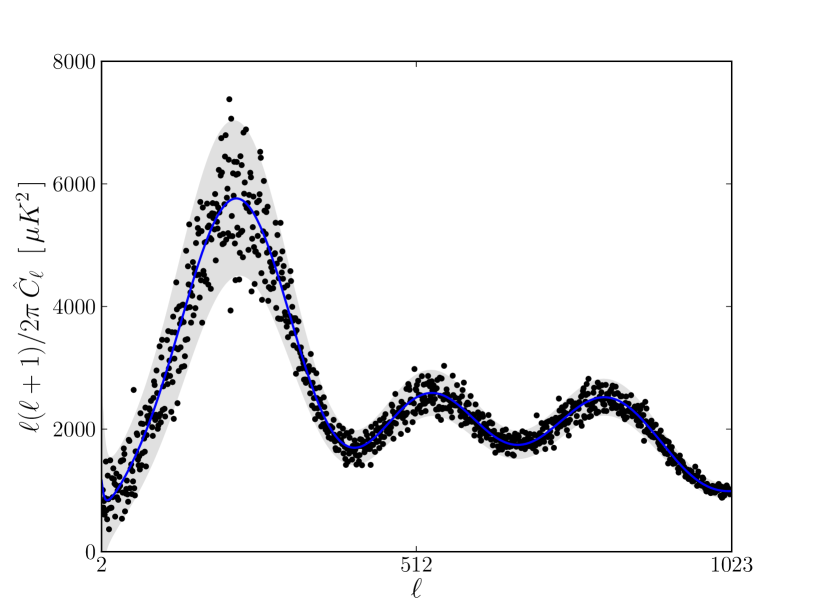
In Fig. 2, we show the estimated maximum likelihood power spectrum of the reference simulation, $\hat{C}_{\ell}$, and compare it to the input we adopted to synthesize the CMB anisotropies. Approximating the likelihood as Gaussian around the peak, we can calculate the goodness of fit using the Fisher matrix $F$ according to

$$\chi^{2}=(\hat{C}_{\ell}-C^{\mathrm{\,Input}}_{\ell})^{\dagger}F\,(\hat{C}_{\ell}-C^{\mathrm{\,Input}}_{\ell})\,.$$ (15)

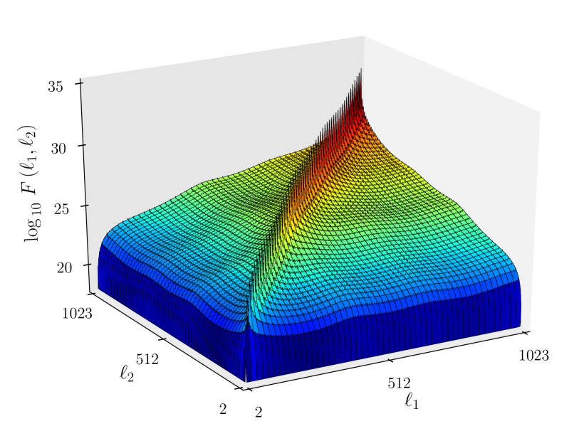
Since monopole and dipole are excluded from the fit, we set $N_{\mathrm{dof}}=\ell_{\mathrm{max}}-1$, and obtain $\chi^{2}/N_{\mathrm{dof}}=1.09$. We conclude that the fiducial model is consistently recovered. The Fisher matrix, depicted in the right hand panel of Fig. 2, exhibits a non-trivial shape with noticeable deviations from a simple diagonal matrix.

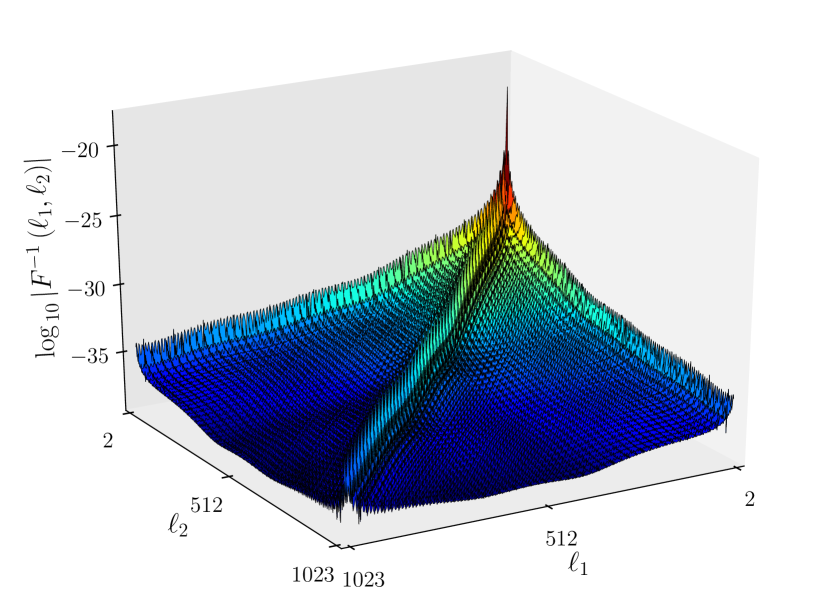
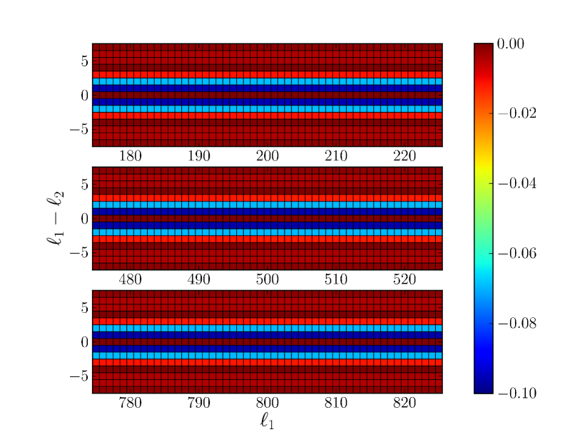
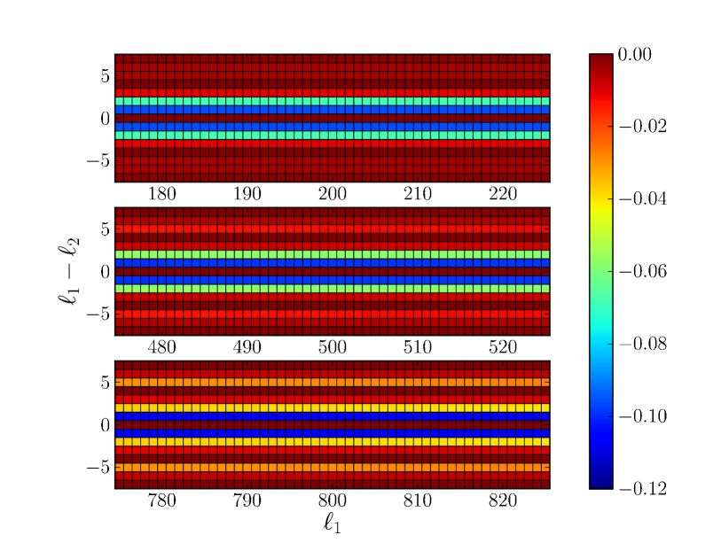
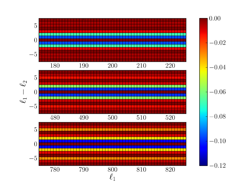
To characterize the correlation structure of the power spectrum, we plot the covariance matrix in Fig. 3. In this diagram, rows or columns at low multipole moments appear to be dominating. However, this effect is the result of the approximate $\ell^{-2}$ scaling of the CMB power spectrum. We therefore use Eq. (13) to normalize the covariance matrix for an unbiased assessment of the correlation structure and find no evidence for an enhanced coupling of small and large scale perturbations. Instead, the normalized correlation matrix is dominated by its diagonal elements which we illustrate at low, intermediate, and high multipoles in the right hand panel of Fig. 3. Obviously, a power spectrum coefficient $C_{\ell}$ shows a substantial negative correlation at the 10 % level with its direct neighbors $C_{\ell\pm 1}$ and $C_{\ell\pm 2}$. Longer-ranging correlations are suppressed to below 1 %. As the signal-to-noise ratio (S/N) is large in the entire multipole range considered here, the evolution of the correlation coefficients towards higher $\ell$ is negligible.

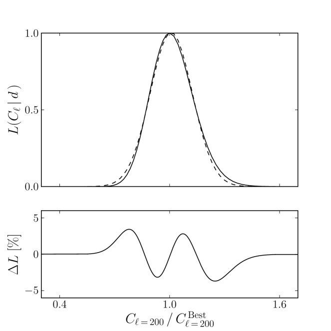
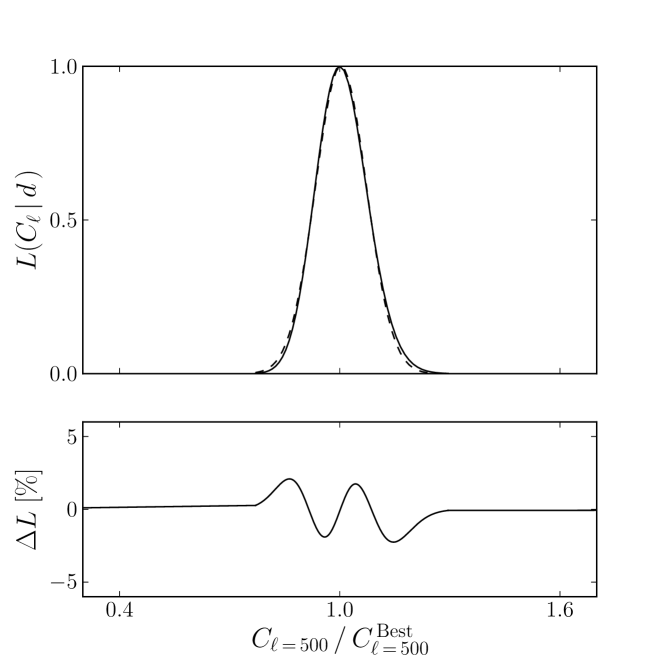
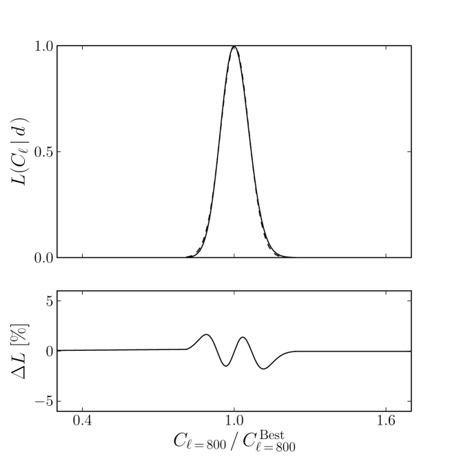
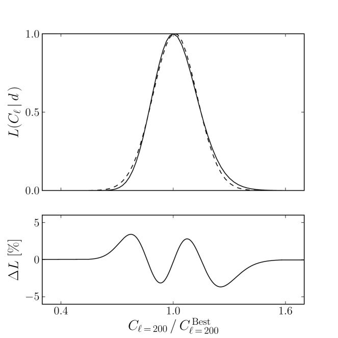
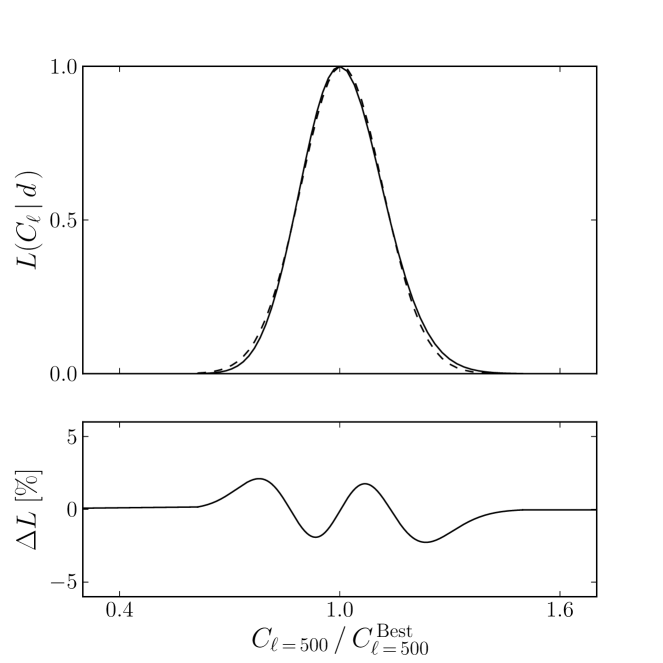
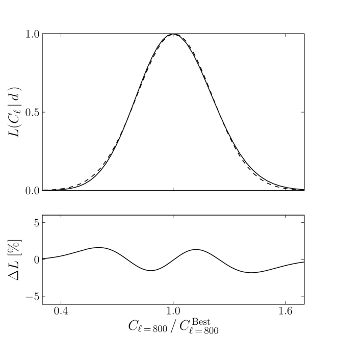
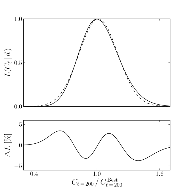
It has been noted before, that the likelihood function is strongly non-Gaussian at the lowest multipole moments (e.g., Bond et al. 1998; Wandelt et al. 2004). As a consequence, exact sampling methods are commonly used for the data analysis in this regime (Hinshaw et al. 2009; Jarosik et al. 2011). However, and in contrast to previous claims in literature, we also find a noticeable deviation from Gaussianity at the highest multipole values. We illustrate the shape of the likelihood function for large, intermediate, and small scale perturbations in Fig. 4. For all power spectrum coefficients, a fit with a simple Gaussian distribution leaves residuals at the level of several percent. Combining the individual errors for each multipole moment, the total error on the likelihood function can be substantial if it is modeled by a simple multivariate Gaussian.

Figure 2: Left panel: The result of an exact maximum likelihood power spectrum estimation (filled circles) shows that the input power spectrum can be consistently recovered (solid line). The gray area indicates the 2-$\sigma$ confidence region as derived from the Fisher matrix. Right panel: The Fisher matrix of the CMB power spectrum coefficients cannot be approximated well by a diagonal matrix.

Figure 3: The correlation structure between power spectrum coefficients is complicated. Left panel: We plot the inverse of the Fisher matrix, i.e. the covariance matrix of the experiment. For illustrative purposes, we inverted the x and y axes. Right panel: Patches around the diagonal elements of the normalized correlation matrix at low ($\ell=200$, upper row), intermediate ($\ell=500$, middle row), and high multipoles ($\ell=800$, lower row) reveal significant negative correlations between neighboring power spectrum coefficients at the 10 % level.

Figure 4: The likelihood is non-Gaussian. Upper row: Varying the power spectrum coefficients for different multipole values, we plot slices of the likelihood function (solid lines) at low ($\ell=200$, left panel), intermediate ($\ell=500$, middle panel), and high multipoles ($\ell=800$, right panel). We also show the best fitting Gaussian distributions (dashed lines). Lower row: The absolute residual between the likelihood function and its Gaussian fit is of the order of several percent.

3.2 The effect of asymmetric beams

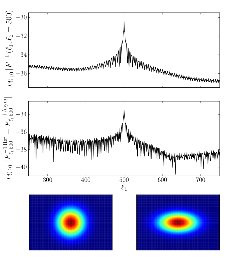
At some level, all CMB experiments suffer from beam imperfections, depending on detector design and focal plane geometry. For the low frequency instrument aboard the Planck satellite, for example, the beam ellipticity can reach 40 % (Mennella et al. 2011). We now study whether asymmetric beams by themselves pose a problem in a sense that they lead to a loss of information or induce additional correlations between power spectrum coefficients. Again, we study the impact of asymmetric beams on the information content that could ultimately be obtained after an optimal analysis of the data.

To this end, we repeated the full likelihood analysis on a data set generated with the simulation parameters as above, except for the fact that we now included an asymmetric Gaussian beam with an axes ratio of $\sigma_{\mathrm{x}}/\sigma_{\mathrm{y}}=2:1$. We kept the geometric mean of the FWHM along the major and minor axis fixed at $12\arcmin$. In Fig. 5, we compare a slice through the covariance matrix of the simulation against our benchmark model. The relative difference of the entries close to the dominating diagonal elements is smaller than 1 %. We conclude that an asymmetric beam per se, if accounted for exactly in the analysis, neither degrades the information content of the experiment, nor complicates the correlation structure of the power spectrum coefficients.

Figure 5: Asymmetric beams do not destroy information. Upper panel: For a multipole moment of $\ell=500$, we show a slice through the covariance matrix for the reference simulation with symmetric beam. Middle panel: The relative difference between the covariance matrices calculated with symmetric beam ($F^{-1\,\mathrm{Ref}}$) and strongly asymmetric beam ($F^{-1\,\mathrm{Asym}}$) is only of the order 1 %. Lower panel: Beam profiles used in the comparison.

3.3 The effect of the noise properties

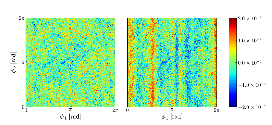
We now characterize the impact of different noise properties on the likelihood function. To be more precise, we first vary the overall noise level without modifying its power spectrum, and then analyze the effect of correlated noise. The data sets used for this study are visualized in Fig. 6.

3.3.1 Low S/N likelihood

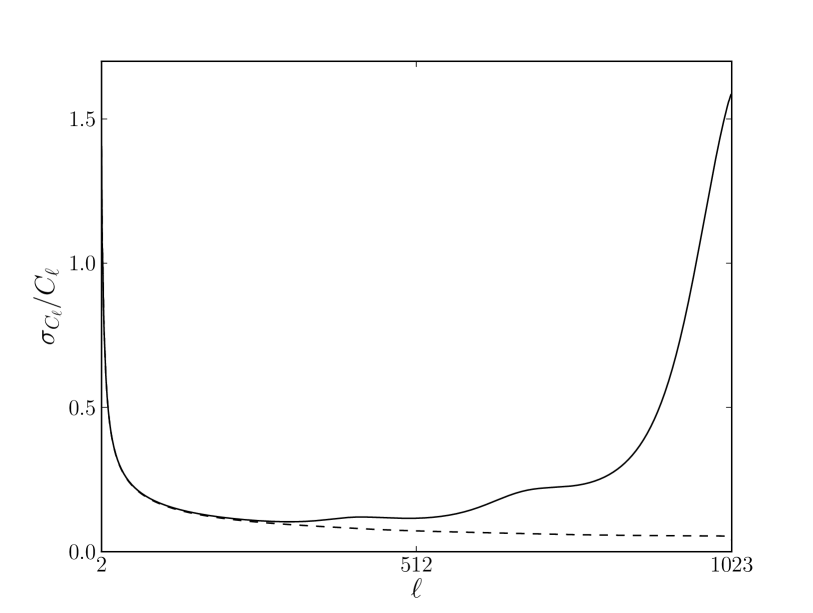
For the analysis of the effect of noise on CMB power spectrum estimation, we increased the noise power spectrum amplitude in Eq. (12) to $\sigma=200$ mK. In this setup, we obtained a S/N of unity at a multipole $\ell\approx 700$. As expected, the diagonal elements of the inverse Fisher matrix reflect the increase in noise (Fig. 7). We also find the correlation structure of the Fisher matrix change qualitatively at high multipoles, it becomes stronger and more complex. In particular, the negative correlation between a power spectrum coefficient $C_{\ell}$ and $C_{\ell\pm 5}$ increases in strength. The full correlation matrix, plotted on logarithmic scale to highlight the off-diagonal entries, is depicted in Fig. 8. Becoming more and more relevant with the decreasing S/N towards higher $\ell$, the inhomogeneously distributed noise induces additional long-ranging correlations between power spectrum coefficients at the sub-percent level. We show likelihood slices in Fig. 9. When compared to the high S/N case in Fig. 4, the analysis reveals a widened distribution at high multipoles. Besides that, the non-Gaussian features of the likelihood function remain basically unchanged. Only a further decrease in the S/N starts to diminish the deviation from a Gaussian shape. In that case, however, the power spectrum coefficients have too large an error bar for them to play a substantial role in the estimation of cosmological parameters.

Figure 6: Data sets used to study the impact of noise. Left panel: We show the data of the low S/N simulation with uncorrelated noise projected onto an unfolded torus. The scan on a single ring proceeds towards larger values of $\phi_{2}$, the ring number increases along the horizontal axis ($\phi_{1}$). Right panel: Low S/N simulation, additionally containing $1/f^{2}$-type noise. Strong correlations extending well beyond individual rings are visible.

Figure 7: Left panel: We compare the Fisher matrix based prediction of the 1-$\sigma$ error bars of the power spectrum coefficients between our benchmark (dashed line) and the simulation with lower S/N and uncorrelated noise (solid line). Right panel: As a plot of the correlation matrix confirms, an increase in noise towards higher multipoles strengthens the amount of correlation and complicates the correlation structure (cf. Fig. 3).

Figure 8: An increased level of noise, distributed inhomogenously over the sky, introduces additional long-range correlations between power spectrum coefficients at the sub-percent level.

Figure 9: Same as Fig. 4, but for a simulation with low S/N. Simply increasing the error bars, additional noise, most noticeable at the highest multipole moment, largely preserves the non-Gaussian features of the likelihood function.

3.3.2 Correlated noise

Next, we study the effect of correlated noise. To this end, we generate a simulation with parameters as follows. Choosing a noise realization with $\alpha=2$ in Eq. (12), we selected a knee frequency of $k_{\mathrm{knee}}=10^{-3}$ in terms of the Nyquist frequency, and set the DC mode to zero. Red noise is often present in experiments to some level, and it also affects the high frequency instrument data of the Planck satellite mission (Planck HFI Core Team et al. 2011). Here, we kept the overall noise power spectrum amplitude at $\sigma=200$ mK, the same level as in the previous scenario. Owing to the additional long-range correlations, the noise variance per pixel in the data map increased considerably (cf. Fig. 6).

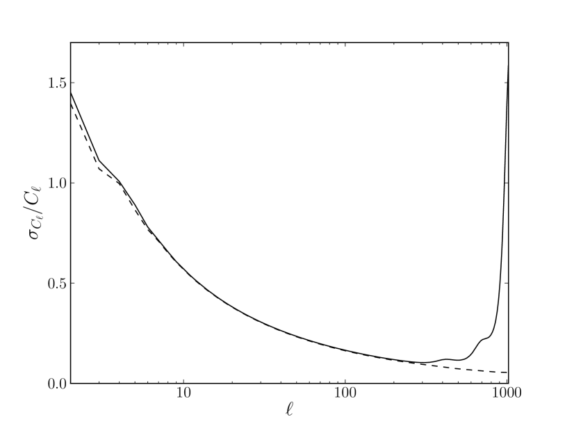
The analysis based on the Fisher matrix is shown in Fig. 10, where we plot the error bars and the correlation matrix of the experiment. The impact of the red noise on the likelihood function is negligible when it is accounted for exactly in the analysis. The additional low-frequency noise contribution, most relevant for large-scale perturbations, still falls within a highly signal dominated regime. As a result, its effect on the power spectrum estimation can be removed efficiently. Only for the smallest multipole moments, $\ell\la 5$, we observe an increase in the error bar by no more than 3 %. Accordingly, the correlation structure between power spectrum coefficients is virtually unaffected.

Figure 10: Same as Fig. 7, but for the simulation containing noise with additional large-scale correlations. The error bars remain at the same level. Only at the largest scales, $\ell<5$, a mild loss of information is apparent. Changes in the normalized correlation matrix are negligible.

3.4 The effect of partial sky coverage

Excluding large parts of the sky from the analysis has the potential to severely complicate power spectrum estimations. This problem roots in the mathematical properties of the spherical harmonics. Restricted to a subdomain of the sphere, the functions do no longer fulfill an orthonormality relation. As a result, correlations between the CMB power spectrum coefficients are induced.

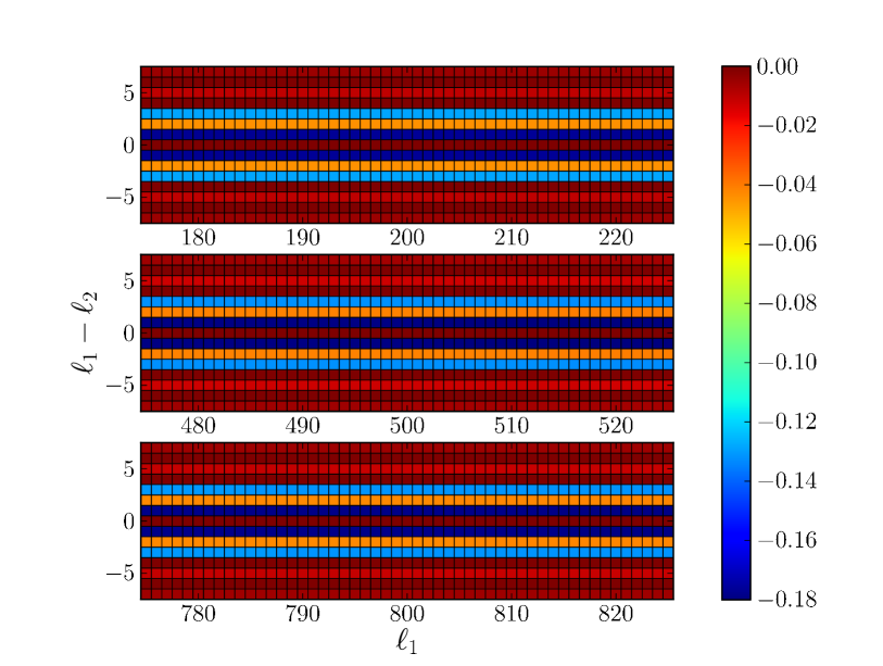
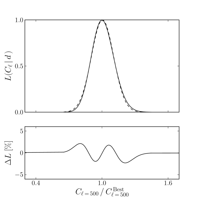
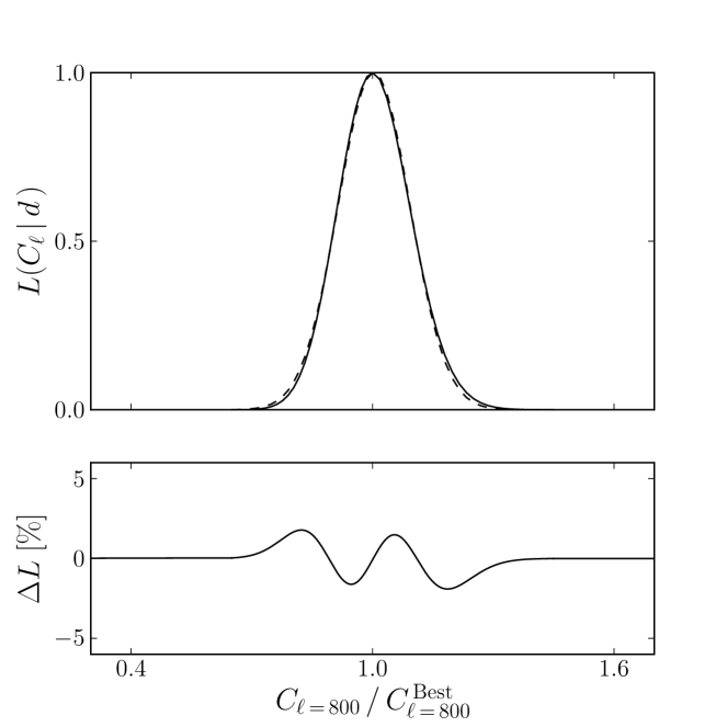
All ground based CMB experiments observe only a fraction of the sky (e.g., Kosowsky 2003; Ruhl et al. 2004). But even for satellite-borne experiments, the contamination by secondary sources necessitates to mask large sky regions in favor of an unbiased CMB power spectrum estimation (e.g., Jarosik et al. 2011). To further study the effect of restricting the observations to a small part of the sky, we analyzed a simulation with a reduced coverage of $f_{\mathrm{sky}}=40\leavevmode\nobreak\ \%$. We chose the simulation parameters of our benchmark data set, except for the opening angle of the scanning rings, which we reduced to $\theta_{\mathrm{o}}=25\degr$. As we still sampled the data with the same number of nodes ($N_{\mathrm{p}}=N_{\mathrm{r}}=2048$), we slightly adapted the noise amplitude to the finer grid to obtain the same S/N in the power spectrum, $\sigma=\sqrt{60\leavevmode\nobreak\ \%/40\leavevmode\nobreak\ \%}\cdot 10\leavevmode\nobreak\ \mathrm{mK}\approx 12.2$ mK. In Fig. 11, we visualize the normalized correlation matrix. A comparison to the right hand panel of Fig. 3 shows an increase in the amplitude of correlation by about a factor of two. In addition, an even/odd asymmetry becomes visible as the power spectrum coefficients $C_{\ell}$ are now negatively correlated with $C_{\ell\pm 3}$ at the 12 % level, whereas the amount of negative correlation for $C_{\ell\pm 2}$ decreases to 5 %. We plot slices of the likelihood in Fig. 12. The loss of information associated with a reduction of sky coverage leads to widened distributions, most noticeable at large angular scales. Interestingly, the non-Gaussian pattern in the likelihood function are remarkably robust and remain at about the same level.

Figure 11: A small sky coverage induces complicated correlations. We plot the normalized correlation matrix for a simulation covering $f_{\mathrm{sky}}=40\leavevmode\nobreak\ \%$ of the sky. A larger mask increases the correlation in strength and range (cf. Fig. 3).

Figure 12: Same as Fig. 4, but for a simulation with larger mask. Lowering the sky coverage from 60 % to 40 % leads to less stringent constraints on the power spectrum coefficients, but has a negligible effect on the amount of deviation of the likelihood function from a Gaussian distribution.

3.5 The effect of binning

As established in the previous paragraph, a large galactic cut induces significant correlations between neighboring power spectrum coefficients. Furthermore, the likelihood function is non-Gaussian to a noticeable extent. As the theoretical power spectrum is a smooth function of only a few cosmological parameters, combining the observed power spectrum coefficients into bins is a common practice in parameter estimation. This approach reduces scatter in the data points and has the potential to simplify the correlation structure. Here, we analyze the effect of binning on the likelihood function.

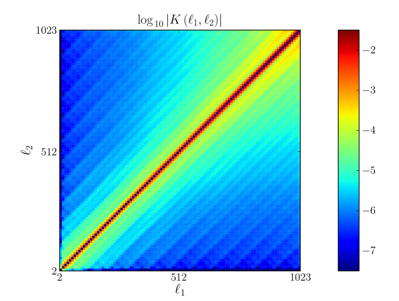
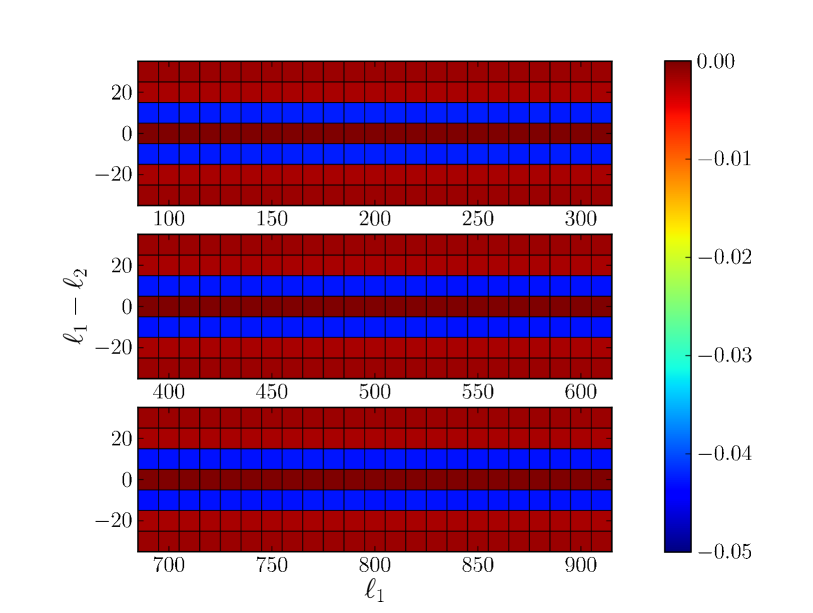
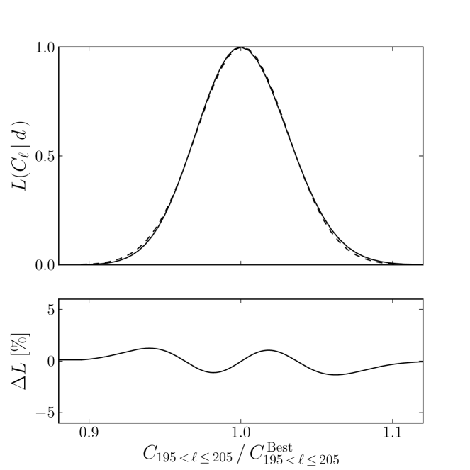
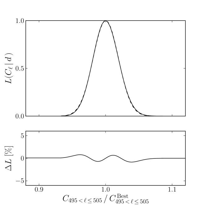
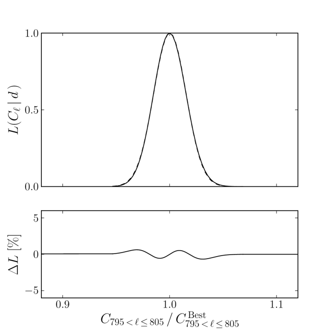
We chose a bin width of $\Delta\ell=10$ and repeated the analysis of our reference simulation. In Fig. 13, we plot the correlation structure of the likelihood function. Neighboring power spectrum bins are still negatively correlated, although at a smaller amount of about 5 %. The bin after next, however, is almost completely decorrelated. Furthermore, the shape of the likelihood function, shown in Fig. 14, can be much better described by a Gaussian distribution, where the residuals of a fit have decreased to a 1 - 2 % level. Obviously, binning has the desirable side effects to simplify the shape and correlation structure of the likelihood function.

Figure 13: Binning simplifies the correlation structure. We show elements of the correlation matrix for a binned power spectrum with a width of $\Delta\ell=10$. Directly neighboring bins are still negatively correlated to a noticeable extent (cf. Fig. 3).

Figure 14: Same as Fig. 4, but for a binned power spectrum. Combining adjacent power spectrum coefficients results in a more Gaussian probability distribution.

4 Discussion and conclusions

Owing to its reduced size compared to a full data map, the power spectrum of the CMB radiation anisotropies is a convenient intermediate stage product in the process of estimating cosmological parameters. Sufficient to completely characterize a Gaussian random field, it contains all of the most fundamental cosmological information present in the data (Jungman et al. 1996; Bond et al. 1997). To construct the probability distributions of the parameters out of the power spectrum requires a precise modeling of their likelihood function. That is, one has to specify the shape of the function, and the correlation between the individual power spectrum coefficients.

Systematic effects, present in all real-world experiments, have the potential to reduce the information content of a data set. In the context of a CMB power spectrum analysis, issues may arise from beam imperfections, incomplete sky coverage, and correlated noise. Here, we conducted a systematic study of the impact of these effects on the ability to constrain the CMB power spectrum. Assuming a simplified scanning strategy that allows for an exact analytical treatment of the problem, we used the Fisher matrix formalism for a quantitative comparison of the information content of different experimental setups. To complement the analysis, we also explored the shape of the likelihood function directly by varying the amplitude of individual power spectrum coefficients. We obtained the following results:

• For a high S/N experiment that covers 60 % of the sky, we found neighboring power spectrum coefficients to be negatively correlated at the 10 % level. Interestingly, the shape of the likelihood function deviated noticeably from a Gaussian distribution, typically by 2 - 5 %. This was true even for the highest multipole values probed in our analysis, $\ell>1000$.

• Increasing the noise contribution changed the correlation structure between different power spectrum coefficients. It became somewhat more pronounced and of longer range. The residuals of a fit of the likelihood function with a Gaussian distribution remained basically the same.

• Treated exactly, the mere presence of correlated noise did not lead to a loss of information. Comparing two simulations with white and colored noise power spectrum, we found $1/f^{2}$-type noise to be efficiently removed. In addition, it did not increase the amount of correlation among the power spectrum coefficients.

• As expected, the impact of a reduced sky coverage on the analysis was most important. To study this effect, we further limited the observed region to 40 % of the sky. As a result, the negative correlation between power spectrum coefficients increased to up to 18 %. The strength of deviation of the likelihood function from Gaussianity, on the other hand, was mainly unaffected.

• If power spectrum coefficients were combined into bins, the correlation structure among them simplified. Typically, only adjacent bins remained correlated at a noticeable level. Furthermore, the shape of the likelihood function became more Gaussian.

• Finally, if asymmetric beams were present but could be accounted for exactly in the analysis, the Fisher matrix remained virtually unchanged compared to an equivalent experiment with symmetric beams. That is, asymmetric beams by themselves do not destroy information.

As a caveat lector, we re-iterate that we calculate an upper bound on the information content provided in these different experimental scenarios assuming that all instrument properties are known well enough that any small remaining uncertainty does not affect these results. This reveals that the quality of a CMB power spectrum measurement does not depend in principle on symmetric beams or the absence of correlated noise. Recovering the information may require sophisticated analysis and sufficient knowledge of the instrument parameters. Nevertheless, this finding might inspire novel, cost-effective experimental designs that embrace beam asymmetries and/or correlated noise as long as these effects are well-calibrated. It would be interesting in follow-up work to quantify the maximally allowable calibration uncertainties for these statements to hold.

On a more practical level our results are useful in analysis of real data sets in several ways: first we point out the level of non-Gaussianity in the power spectrum likelihood that remains even for relatively large sky coverage and at high $\ell$. We also illustrate the typical correlation structure for measurements with an anisotropic noise distribution. Third, these benchmarks help determine the point of diminishing returns, i.e. when it no longer pays off to refine the data analysis of a real data set. That point is reached when the information recovered from the data set reaches a substantial fraction of the theoretical information bound we give here.