Current-induced atomic dynamics, instabilities, and Raman signals:
Quasi-classical Langevin equation approach

Abstract

We derive and employ a semi-classical Langevin equation obtained from path-integrals to describe the ionic dynamics of a molecular junction in the presence of electrical current. The electronic environment serves as an effective non-equilibrium bath. The bath results in random forces describing Joule heating, current-induced forces including the non-conservative wind force, dissipative frictional forces, and an effective Lorentz-like force due to the Berry phase of the non-equilibrium electrons. Using a generic two-level molecular model, we highlight the importance of both current-induced forces and Joule heating for the stability of the system. We compare the impact of the different forces, and the wide-band approximation for the electronic structure on our result. We examine the current-induced instabilities (excitation of runaway “waterwheel” modes) and investigate the signature of these in the Raman signals.

I Introduction

The interaction of electrons with local vibrations (phonons) has an important impact on the conduction properties and stability of molecular conductorsReed et al. (1997); Smit et al. (2002); Rubio et al. (1996); Yanson et al. (1998); Ohnishi et al. (1998) and has undergone intense study both experimentally and theoreticallyPascual et al. (2003); Tao (2006); Lindsay and Ratner (2007); Galperin et al. (2008); Schulze et al. (2008); Galperin et al. (2007); Horsfield et al. (2006); Stipe et al. (1998); Agraït et al. (2003, 2002); Park et al. (2000); Viljas et al. (2005); Frederiksen et al. (2004); Paulsson et al. (2005); Frederiksen et al. (2007); Paulsson et al. (2008); Sergueev et al. (2005); Pecchia et al. (2007); McEniry et al. (2007); Chen et al. (2003); Todorov (1998); Segal and Nitzan (2002); Huang et al. (2007); Ness et al. (2001); Braig and Flensberg (2003); Mitra et al. (2004); Härtle et al. (2009); Lorente et al. (2001); Mii et al. (2003); Asai (2008); Lü and Wang (2007); Jiang et al. (2005); Kushmerick et al. (2004); Galperin et al. (2006); Tsutsui et al. (2008); Verdozzi et al. (2006); Hihath et al. (2008); Smit et al. (2004); Tsutsui et al. (2006); Stamenova et al. (2006); Zhang et al. (2011); Jorn and Seideman (2009, 2010). In the low bias regime where the voltage is comparable to phonon excitation energies, valuable information about the molecular conductor can be deduced from the signature of electron-phonon interaction, known as inelastic electron tunneling spectroscopy (IETS), or point contact spectroscopy (PCS)Smit et al. (2002); Agraït et al. (2002); Okabayashi et al. (2010); Fock et al. (2011); Kim et al. (2011). Theoretically, this regime has been addressed with some success using mean-field theory such as density functional theoryFrederiksen et al. (2004); Paulsson et al. (2005); Frederiksen et al. (2007); Paulsson et al. (2008); Sergueev et al. (2005); Pecchia et al. (2007); Jiang et al. (2005); Okabayashi et al. (2010), where the vibrations are assumed to be uncoupled to the electrons, while the effect of the phonons on the electronic transport is taken into account using perturbation theory. On the other hand, for higher voltage bias, and for highly transmitting systems, a large electronic current may strongly influence the behavior of the phonons even for relatively weak electron-phonon coupling. The resultant “Joule heating” is well-known in the molecular electronics contextTodorov (1998); Tao (2006); Galperin et al. (2007); Horsfield et al. (2006), and remains a lively area with a range of approaches (and with occasional lack of complete agreement between treatments McEniry et al. (2007); Chen et al. (2003)).

More recently the current-induced wind-force known from electromigrationSorbello (1998) has been reexamined for atomic-scale conductors and shown also to be able to excite the conductor and possibly lead to a runaway instabilityDundas et al. (2009); Todorov et al. (2010); Lü et al. (2010); Todorov et al. (2011); Lü et al. (2011a); Bode et al. (2011, 2012). It has been shown how a part of the force on an atom in the presence of the current may have a non-conservative (NC) component, able to do net work around closed paths. This was explicitly proven by calculating the curl of the vector field describing the force on an atomDundas et al. (2009); Todorov et al. (2011). The NC energy transfer - also dubbed the atomic “waterwheel” effect - requires a generalized circular motion of the atoms and involves the coupling of the electronic current to more than one vibrational mode.

Along with the NC force contribution we have recently identified a velocity-dependent current-induced force which conserves energy and acts as a Lorentz-like force on the generalized circular motion. This force can be traced back to the quantum mechanical Berry-phase (BP) of the electronsLü et al. (2010); Bode et al. (2012). Together with the NC force we will, further, have a component which is curl-free and is related to the change in the effective potential energy surface of the atoms due to the currentDzhioev and Kosov (2011); Nocera et al. (2011), as well as nonadiabatic “electronic friction” forcesHead-Gordon and Tully (1995). In the nonequilibrium situation the “friction” force can, however, turn into a driving force amplifying the vibration. This happens under certain resonance conditions akin to a laser effect, but now involving phonons instead of photonsLü et al. (2011b); Bode et al. (2011).

A unified approach including all aforementioned effects on an equal footing is highly desirable for further study in this direction. In this paper, we extend the electronic friction approach proposed by Head-Gordon and TullyHead-Gordon and Tully (1995) for molecular dynamics to take into account the nonequilibrium nature of the electronic currentBrandbyge and Hedegård (1994); Brandbyge et al. (1995); Mozyrsky et al. (2006); Lü et al. (2010); Nocera et al. (2011); Bode et al. (2012). A similar approach has been taken to describe models of nano-electro-mechanical systems (NEMS)Hussein et al. (2010); Metelmann and Brandes (2011). Using the Feynman-Vernon influence functional approach, we derive a semi-classical Langevin equation for the ions, which we can use to study Joule heating, current-induced forces, and heat transport in molecular conductors. We perform a perturbation expansion of the electron effective action over the electron-phonon interaction matrix. This allows us to make connections with other theoretical approaches, especially the nonequilibrium Green’s function (NEGF) method, used to study the Joule heating problemFrederiksen et al. (2007); Pecchia et al. (2007). We also give an extension of the perturbation result to the adiabatic limit, which makes connections with our previous results, and solves an infrared divergence problem in the expression of the BP force in Ref. Lü et al., 2010. We apply the theory to a two-level model in order to (1) clarify the roles played by different forces regarding the stability of the device, and (2) discuss the signature of the current-induced excitation in the Raman-scattering especially focussing on conditions close to a current-induced runaway instability.

The paper is organized as follows. In Sec. II we briefly review the derivation of the generalized Langevin equation. In Sec. III we analyse the electronic forces entering into the Langevin equation. Sec. IV compares the effect of different current-induced forces for a two-level model, concentrating on the NC and BP force. In Sec. V, we extend the perturbation result to the adiabatic limit, and introduce coupling of the system with electrode phonons. The derived formulas can be used to study the current-induced phononic heat transport. In Sec. VI, we present ways of calculating the quantum displacement correlations, which is essential for the theoretical description of Raman spectroscopy in the presence of current. Section VII gives concluding remarks.

II Theory

II.1 Influence functional theory

We start from the influence functional theory of Feynman and Vernon Feynman and Vernon (1963), which treats the dynamics of a “system” in contact with a “bath” or “reservoir”. In our case the system of interest consists of the few degrees of freedom describing the ions of a molecular conductor, interacting with the electronic reservoir composed of all electronic degrees of freedom in the molecule and electrodes, as well as the phonon reservoirs of two electrodes. The reservoirs can be out of equilibrium generating an electronic current, and may, further, involve a temperature difference generating a heat flux between the electrodes. All effects of the bath are included in the so-called influence functional, which gives an additional effective action, modifying that of the isolated system.

Now we briefly review the idea of the influence functional approach. With the help of the influence functional, $F$, the reduced density matrix of the system in the displacement representation reads,

$$\langle x_{2}|\rho_{s}(t_{2})|y_{2}\rangle = \int dx_{1}\int dy_{1}\mathcal{K}(x_{2},y_{2};x_{1},y_{1})$$ (1)

$$\times\langle x_{1}|\rho_{s}(t_{1})|y_{1}\rangle,$$

with the propagator of the reduced density matrix

$$\mathcal{K}(x_{2},y_{2};x_{1},y_{1}) = \int_{(x,y)(t_{1})=(x_{1},y_{1})}^{(x,y)(t_{2})=(x_{2},y_{2})}{\cal D}(x,y)$$ (2)

$$\times {\rm exp}\left[\frac{i}{\hbar}\left(S_{s}(x)-S_{s}(y)\right)\right]F(x,y).$$

Here $x$ and $y$ are a pair of displacement histories of the ions, and $S_{s}$ is the action of the system only. In deriving this, we have assumed that the system and bath are uncorrelated at $t_{1}(\to-\infty)$,

$$\rho(t_{1})\>=\>\rho_{s}(t_{1})\>\otimes\>\rho_{b}(t_{1}).$$ (3)

The influence functional includes the information of the bath $S_{b}$ and its interaction with the system $S_{i}$,

$$F(x,y)=\int d{r_{2}}d{r_{1}}d{q_{1}}\int_{(r,q)(t_{1})=(r_{1},q_{1})}^{(r,q)(t_{2})=(r_{2},r_{2})}{\cal D}(r,q)$$

$$\times{\rm exp}\left[\frac{i}{\hbar}\left(S_{b}(r)+S_{i}(x,r)-S_{b}(q)-S_{i}(y,q)\right)\right]$$

$$\times\langle r_{1}|\rho_{b}(t_{1})|q_{1}\rangle.$$ (4)

with $r$ and $q$ representing forward and backward paths of the bath degrees of freedom. Most importantly, a correction to the action of the system can be defined from the influence functional $\Delta S=-i\hbar\,\ln F(x,y)$, which is usually not time-local or real. It has been used to derive a semiclassical Langevin equation, describing the dynamics of the system interacting with the environmentCaldeira and Leggett (1983); Schmid (1982). In this case new variables are introduced,

$$Q=\frac{1}{2}(x+y),\quad\quad\xi=x-y\,,$$ (5)

describing the average and difference of the two paths, respectively. In the semi-classical approach the average path, $Q$, is shown to yield the variable in the Langevin equation, whereas role of the difference, $\xi$, is to introduce fluctuating random forces in a statistical interpretation. The influence of the environment will favor paths with small excursions given by $\xi$, and will ensure that only the solution, $Q$, obeying the classical path will contribute for a high temperature reservoir. We illustrate this further below.

Next, we introduce our model and give the result for the influence functional describing the nonequilibrium electron bath. From the effective action, we can read out the forces acting on the ions due to the electrons. We also discuss how a thermal flux may be included. Parts of the derivations can be found in our previous publicationsBrandbyge and Hedegård (1994); Brandbyge et al. (1995); Lü et al. (2010), but here we aim at a more general formulation, which we present with detailed derivations together with an illustrative model calculation. However we note that the theory is fully compatible with more realistic systems with complex electronic and vibrational structure treated within a mean-field approach such as density functional theory.

II.2 System setup and Hamiltonian

To obtain an effective action describing the vibrations (phonons) in the molecular conductor we first divide the complete system into electron and phonon subsystems. We will treat electron-electron interactions at the mean-field level. To describe the nonequilibrium situation where a current is flowing through the molecular conductor between two reservoirs, the electron subsystem is further divided into a cental part ($C$) and two electrodes ($L,R$), whose electrochemical potentials change with applied bias. For the purposes of the present study, we allow electrons to interact with phonons in $C$ only, and furthermore ignore the anharmonic coupling between these different modes. The coupling of the molecular vibrations with electrode phonons will be considered in Sec. V.2.

The single particle mean-field electronic Hamiltonian at the relaxed ionic positions, ${H}^{0}$, is written within a tight-binding or LCAO type basis with corresponding electron creation (annihilation) operators for the $j$th orbital, $c^{\dagger}_{j}$ ($c_{j}$). The Hamiltonian $H^{0}$ spans the whole $LCR$ system, while the electron-phonon interaction is localized in $C$ Frederiksen et al. (2007). The Hamiltonian of the whole system reads,

$${H} = {H}_{ph}+{H}_{e}({u}),$$ (6a)

$${H}_{ph} = \frac{1}{2}p^{T}p+\frac{1}{2}u^{T}Ku,$$ (6b)

$${H}_{e}({u}) = \sum_{i,j}H^{0}_{ij}{c}^{\dagger}_{i}{c}_{j}+\sum_{k,i,j\in C}M^{k}_{ij}{c}^{\dagger}_{i}{c}_{j}{u}_{k},$$ (6c)

where $p$ are momenta conjugate to $u$, and $u$ is a column vector containing the mass-normalized displacement operators of all ionic degrees of freedom (e.g. $u_{k}=\sqrt{m_{k}}(r_{k}-r^{0}_{k})$, where $m_{k}$ is the mass of ionic degree of freedom $k$ and $r_{k}$ ($r^{0}_{k}$) is its (equilibrium) position). The equilibrium zero-current dynamical matrix is denoted by $K$. This Hamiltonian has been used to describe IETS in molecular contacts with parameters obtained e.g. with DFT for concrete systemsFrederiksen et al. (2007); Okabayashi et al. (2010). We have previously discussed the adiabatic limit, where the perturbation is in terms of the velocities $\dot{u}_{k}$ and where the full non-linear effects of $u_{k}$ can be included. Here we instead assume small displacements from equilibrium and expand the electronic Hamiltonian to first order in $u_{k}$. Later in Sec. V.1 we compare this to the adiabatic limit, discussed in Refs. Lü et al., 2010; Bode et al., 2012.

The correction to the action due to the coupling to the electron reservoirs can be found using the linked-cluster expansion in the coupling, $M^{k}$, following Ref. Brandbyge et al., 1995. The effective action of the nonequilibrium, noninteracting electron bath reads,

$$\Delta S(x,y) = i\hbar\sum_{k}\int_{0}^{1}d\lambda\int_{K}d\tau\;$$ (7)

$$\times {{\rm Tr}}[{{G}}(\tau,\tau_{+};{X}){M}^{k}{X}_{k}(\tau)]\;,$$

where the trace ${\rm Tr}\left[\right]$ is over the electronic bath and this will be so in all following formulas. The parameter $\lambda$ is used to keep track of the order in the linked-cluster expansionMahan (1990). The time $\tau$ is defined on the Keldysh contourHaug and Jauho (2008) $K$. On the real time axis the Green’s function decomposes into

$${{G}}(\tau,\tau^{\prime})\>=\>\left(\begin{array}[]{cc}{G}(t,t^{\prime})&{G}^{<}(t,t^{\prime})\\ {G}^{>}(t,t^{\prime})&{\bar{G}}(t,t^{\prime})\end{array}\right),$$ (8)

and

$${X}(\tau)\>=\>\left(\begin{array}[]{cc}x(t)&0\\ 0&-y(t)\end{array}\right).$$ (9)

Time $\tau_{+}$ is infinitesimally later than $\tau$ on the whole Keldysh contour. The limits of integration extend to $-\infty$ and $+\infty$ if not specified. This applies to all the integrals in the paper. The Green’s function is given by the Dyson equation,

$${{G}}(\tau,\tau_{+})={{G}}_{0}(\tau,\tau_{+})$$

$$+ \sum_{k}\int_{K}d\tau^{\prime}{{G}}_{0}(\tau,\tau^{\prime}){{M}^{k}}{{X_{k}}}(\tau^{\prime}){{G}}(\tau^{\prime},\tau_{+}),$$

${{G}}_{0}$ being the single electron Green’s function without interaction with the ions, which reads

$${{G}}_{0}(\tau,\tau^{\prime})=i\sum_{\alpha}\int\frac{d\varepsilon}{2\pi\hbar}\;e^{-\frac{i}{\hbar}\varepsilon(t-t^{\prime})}A_{\alpha}(\varepsilon)\times$$ (11)

$$\left(\begin{array}[]{cc}n_{F}(\varepsilon-\mu_{\alpha})-\theta(t-t^{\prime})&n_{F}(\varepsilon-\mu_{\alpha})\\ n_{F}(\varepsilon-\mu_{\alpha})-1&n_{F}(\varepsilon-\mu_{\alpha})-\theta(t^{\prime}-t)\end{array}\right).$$ (14)

$n_{F}(\varepsilon-\mu_{\alpha})=1/\left[1+e^{(\varepsilon-\mu_{\alpha})/k_{B}T}\right]$ is the Fermi-Dirac distribution function for electrode $\alpha$, $A=\sum_{\alpha}A_{\alpha}$, and $\theta$ is the Heaviside step function. The spectral function is defined as

$$A_{\alpha}(\varepsilon)=iG_{0}^{r}(\varepsilon)[\Sigma^{r}_{\alpha}(\varepsilon)-\Sigma_{\alpha}^{a}(\varepsilon)]G_{0}^{a}(\varepsilon),$$ (15)

and $\Sigma^{r}_{\alpha}(\varepsilon)$ ($\Sigma^{a}_{\alpha}(\varepsilon)$) the retarded (advanced) electron self-energy from lead $\alpha$. We use $\varepsilon$ and $\omega$ as parameters for the electron and electron-hole pair/phonon properties, respectively.

The effective action in Eq. (7) could be expanded into an infinite series in $M$. We only keep terms up to second order, assuming small $M$ (or alternatively assuming small displacements as stipulated earlier). The first-order contribution written in terms of the average and difference paths for the vibrations, $Q_{k},\xi_{k}$, reads,

$$\Delta S^{(1)}(Q,\xi) = \sum_{k}F^{(1)}_{k}\>\int dt\;\xi_{k}(t),$$ (16)

with a first-order, displacement-independent force term,

$$F^{(1)}_{k}=-2\sum_{\alpha}\int\frac{d\varepsilon}{2\pi}\;{{\rm Tr}}[A_{\alpha}(\varepsilon)M^{k}]\Delta n^{\alpha}_{F}(\varepsilon),$$ (17)

$$\Delta n^{\alpha}_{F}(\varepsilon)=n_{F}(\varepsilon-\mu_{\alpha})-n_{F}(\varepsilon-\mu_{0}).$$ (18)

Here $\mu_{0}$ is the equilibrium electrochemical potential and the factor of $2$ accounts for spin degeneracy. Above we explicitly subtract the equilibrium forces (obtained for $\mu_{\alpha}=\mu_{0}$), since these are already included in the elastic forces described by $K$. The different filling of electronic states originating from different electrodes in Eq. (18) results in a displacement-independent “wind” forceSorbello (1998); Brandbyge et al. (2003); Bevan et al. (2010). Its effect amounts in the small-displacement approximation used here to a bias-induced shift of the equilibrium ionic positions. We will therefore ignore it from now on, since we will be considering the effects of the nonequilibrium electrons on the ionic dynamics.

Before introducing the second-order contribution, we note that the applied bias between the two electrodes also modifies the electronic Hamiltonian, and thus $A_{\alpha}$ and $M^{k}$. It is the result of charge rearrangement in the device in response to the applied bias. This is out of the scope of present paper, and is not included in Eq. (18). The inclusion of external electric fields in the electronic Hamiltonian can account, for example, for the “direct” electromigration forceSorbello (1998).

We now turn to the second-order contribution central to our discussion,

$$\Delta S^{(2)}(Q,\xi)=-\frac{i}{4}\sum_{\alpha,\beta,l,k}\int dt\int dt^{\prime}\;\int d\omega\;$$ (19)

$$\times e^{-i\omega(t-t^{\prime})}\>\Lambda_{kl}^{\alpha\beta}(\omega)\Bigg{[}\coth\left(\frac{\hbar\omega-(\mu_{\alpha}-\mu_{\beta})}{2k_{B}T}\right)$$

$$\times \xi_{k}(t)\xi_{l}(t^{\prime})+2\theta(t-t^{\prime})\xi_{k}(t)Q_{l}(t^{\prime})$$

$$- 2\theta(t^{\prime}-t)\xi_{l}(t^{\prime})Q_{k}(t)\Bigg{]},$$

where the central quantity is an interaction-weighted electron-hole pair density of states (incl. spin),

$$\Lambda^{\alpha\beta}_{kl}(\omega) = 2\int\frac{d\varepsilon_{1}}{2\pi}\;\int\frac{d\varepsilon_{2}}{2\pi}\;\delta(\hbar\omega-\varepsilon_{1}+\varepsilon_{2})\;$$

$$\times {{\rm Tr}}[M^{k}A_{\alpha}(\varepsilon_{1})M^{l}A_{\beta}(\varepsilon_{2})]$$

$$\times (n_{F}(\varepsilon_{1}-\mu_{\alpha})-n_{F}(\varepsilon_{2}-\mu_{\beta})).$$

It has the following properties,

$$\Lambda^{\alpha\beta}_{kl}(\omega)={\Lambda^{\alpha\beta}_{lk}}^{*}(\omega),$$ (21)

$$\Lambda^{\alpha\beta}_{kl}(\omega)=-\Lambda^{\beta\alpha}_{lk}(-\omega),$$ (22)

$$\Lambda(-\omega)=-\Lambda^{*}(\omega),$$ (23)

where we have defined $\Lambda=\sum_{\alpha,\beta}\Lambda^{\alpha\beta}$.

II.3 The generalised Langevin equation

In order not to complicate the equations we will in the following suppress the phonon-mode index and implicitly write vectors and matrices without these. Note that these phonon indices are generally not interchangeable. This calls for care for example when carrying out permutations within the trace in $\Lambda^{\alpha\beta}_{kl}$ and quantities derived from it. If the reader wishes to make such rearrangements, it is necessary to reinstate the indices ($k$, $l$ above), in the correct starting order, first. Using the results of Subsec. II.1 we get the path-integral,

$$\mathcal{K} = \int\mathcal{D}\xi\int\mathcal{D}Q\exp\left[-\frac{i}{\hbar}\int dt\int dt^{\prime}\xi^{T}(t)L(t,t^{\prime})Q(t^{\prime})\right]$$ (24)

$$\times \exp\left[-\frac{1}{2\hbar}\int dt\int dt^{\prime}\xi^{T}(t)\hat{\Pi}(t-t^{\prime})\xi(t^{\prime})\right].$$

We have defined

$$L(t,t^{\prime})=\left(\frac{\partial^{2}}{\partial t^{2}}+K\right)\delta(t-t^{\prime})+{\Pi}^{r}(t-t^{\prime}),$$ (25)

$$\tilde{\Pi}(t-t^{\prime})=2\pi i\,\mathcal{F}^{-1}\{\Lambda(\omega)\},$$ (26)

$${\Pi}^{r}(t-t^{\prime})=\theta(t-t^{\prime})\tilde{\Pi}(t-t^{\prime}),$$ (27)

and

$$\hat{\Pi}(t-t^{\prime})=\mathcal{F}^{-1}\{\hat{\Pi}(\omega)\},$$ (28)

with

$$\hat{\Pi}(\omega)\equiv\hat{\Pi}_{0}(\omega)+\Delta\hat{\Pi}(\omega)$$

$$=-\pi\Lambda(\omega)\coth\left(\frac{\hbar\omega}{2k_{B}T}\right)-\pi\sum_{\alpha\beta}\Lambda^{\alpha\beta}(\omega)$$

$$\times\left[\coth\left(\frac{\hbar\omega-(\mu_{\alpha}-\mu_{\beta})}{2k_{B}T}\right)-\coth\left(\frac{\hbar\omega}{2k_{B}T}\right)\right].$$ (29)

We have split $\hat{\Pi}$ into two terms. We will see in Sec. V.2 that $\Delta\hat{\Pi}$ is responsible for the heating effect. The Fourier transform is defined as $\mathcal{F}\{f(t)\}=\int dtf(t)e^{i\omega t}$, and $\mathcal{F}^{-1}\{f(\omega)\}=\int\frac{d\omega}{2\pi}f(\omega)e^{-i\omega t}$. After a Hubbard-Stratonovich transformation, we get

$$\mathcal{K} = \int\mathcal{D}\xi\int\mathcal{D}Q\int\mathcal{D}f$$ (30)

$$\times \exp\left(\frac{i\xi^{T}_{2}\dot{Q}_{2}}{\hbar}\right)\exp\left(-\frac{i\xi^{T}_{1}\dot{Q}_{1}}{\hbar}\right)$$

$$\times \exp\left[-\frac{i}{\hbar}\int dt\,\xi^{T}(t)\left(\int dt^{\prime}L(t,t^{\prime})Q(t^{\prime})-f(t)\right)\right]$$

$$\times \exp\left[-\frac{1}{2\hbar}\int dt\int dt^{\prime}f^{T}(t)\hat{\Pi}^{-1}(t,t^{\prime})f(t^{\prime})\right].$$

The factors in line 2 (where $\xi_{1}=\xi(t_{1})$, etc) arise from the integration by parts to transform the kinetic energy ($\dot{\xi}^{T}(t)\dot{Q}(t)$) into the form in line 3, and are needed for example if one wishes to make a connection with the Wigner function. The above form of the effective action suggests a classical interpretation to the motion of the average displacement $Q$. It follows a generalized Langevin equationCaldeira and Leggett (1983); Schmid (1982)

$$\ddot{Q}(t)\!=\!-KQ(t)-\!\int{\Pi}^{r}(t-t^{\prime})Q(t^{\prime})dt^{\prime}+f(t),$$ (31)

where $f(t)$ is a classical stochastic force, whose time-correlation is given by

$$\langle f(t)f^{T}(t^{\prime})\rangle=\hbar\hat{\Pi}(t-t^{\prime}).$$ (32)

Equation (31) is the equation of motion for harmonic oscillators, perturbed by the second and third terms due to interaction with electrons. There are two ways of seeing how it arises. First, it is the Euler-Lagrange equation of motion for the action in Eq. (30). Alternatively, if in (30) we carry out the $\xi$-integral, that introduces $\delta(L\cdot Q-f)$ (where $\cdot$ denotes time-integration for short) in the integrand, which restricts $Q(t)$ to the evolutionary path generated by (31). The physical significance of $Q(t)$ is that it is the quasi-classical coordinate appearing in the Wigner function. Its Newtonian equation of motion above relies on the quadratic nature of the effective action as a functional of the generalised coordinates, and would have to be revisited in the presence of higher-order terms in the Hamiltonian, or in the Green’s function expansion.

It is possible to solve the generalised Langevin equation by Fourier transform. From that, we get the semi-classical displacement correlation function,

$$\frac{1}{\hbar}\,\langle QQ^{T}\rangle(\omega)=D^{r}(\omega)\hat{\Pi}(\omega)D^{a}(\omega).$$ (33)

Here the phonon retarded Green’s function is defined as

$$D^{r}(\omega)=(D^{a}(\omega))^{\dagger}=\left[(\omega+i0^{+})^{2}-K-\Pi^{r}(\omega)\right]^{-1}.$$ (34)

Note that $\tilde{\Pi}$ and $\hat{\Pi}$ can be written as the standard phonon self-energies in the NEGF method

$$\tilde{\Pi}(\omega)=\Pi^{r}(\omega)-\Pi^{a}(\omega)=\Pi^{>}(\omega)-\Pi^{<}(\omega),$$ (35)

$$\hat{\Pi}(\omega)=\frac{i}{2}\left[\Pi^{>}(\omega)+\Pi^{<}(\omega)\right].$$ (36)

The self-energy diagram is shown in Fig. 1, and their expressions are given in Appendix C.

Figure 1: Lowest order phonon self-energy due to interaction with electrons.

III Forces

III.1 General results

The electronic forces in the Langevin equation are divided into stochastic and deterministic parts. The correlation function of the stochastic force has the following properties:

$$\hat{\Pi}^{\dagger}(\omega) = \hat{\Pi}(\omega),$$ (37a)

$$\hat{\Pi}(-\omega) = \hat{\Pi}^{*}(\omega).$$ (37b)

Consequently, $\hat{\Pi}(t)$ is real, but in general $\hat{\Pi}(-t)\neq\hat{\Pi}(t)$ at finite bias.

Now let us look at the deterministic forces due to electrons. $\tilde{\Pi}(\omega)$ has the properties:

$$\tilde{\Pi}^{\dagger}(\omega)=-\tilde{\Pi}(\omega),$$ (38a)

$$\tilde{\Pi}(-\omega)=\tilde{\Pi}^{*}(\omega).$$ (38b)

In the Fourier domain, we can split it into different contributions,

$$-\Pi^{r}(\omega)=-i\pi{\rm Re}\Lambda(\omega)+\pi{\rm Im}\Lambda(\omega)$$

$$-\pi\mathcal{H}\{{\rm Re}\Lambda(\omega^{\prime})\}(\omega)-i\pi\mathcal{H}\{{\rm Im}\Lambda(\omega^{\prime})\}(\omega),$$ (39)

where the Hilbert transform is defined as $\mathcal{H}\{g(x^{\prime})\}(x)=\frac{1}{\pi}\mathcal{P}\int\frac{g(x^{\prime})}{x^{\prime}-x}dx^{\prime}$. Using the symmetry properties of $\Lambda(\omega)$, we can now examine each term in Eq. (III.1).

The first term is imaginary and symmetric. It describes the standard friction, i.e. processes whereby the motion of vibrating ions generate electron-hole pairs in the electronic environment. This process exists also in equilibrium. We can write

$$F_{FR}=-\eta(\omega)\dot{Q}(\omega),$$ (40)

with the friction matrix defined by,

$$\eta(\omega)=-\frac{\pi}{\omega}{\rm Re}\Lambda(\omega).$$ (41)

The second term in Eq. (III.1) is real and anti-symmetric. It has a finite value even in the limit of zero frequency. It is describing the NC force, discussed recentlyDundas et al. (2009); Lü et al. (2010); Todorov et al. (2010); Bode et al. (2011); Todorov et al. (2011); Bode et al. (2012)

$$F_{NC}=\mathcal{N}(\omega)Q(\omega),$$ (42)

with

$$\mathcal{N}(\omega)=\pi{\rm Im}\Lambda(\omega).$$ (43)

The third term is real and symmetric, and can be considered a renormalization (RN) of the dynamical matrix

$$F_{RN}=-\zeta(\omega)Q(\omega),$$ (44)

with

$$\zeta(\omega)=\pi\mathcal{H}\{{\rm Re}\Lambda(\omega^{\prime})\}(\omega).$$ (45)

Finally, the last term is imaginary and anti-symmetric, proportional to $\omega$ for small frequencies. Hence it is to be identified with the BP force in Ref. Lü et al., 2010,

$$F_{BP}=-\mathcal{B}(\omega)\dot{Q}(\omega),$$ (46)

with the effective magnetic field

$$\mathcal{B}(\omega)=-\frac{\pi}{\omega}\mathcal{H}\{{\rm Im}\Lambda(\omega^{\prime})\}(\omega).$$ (47)

III.2 Equilibrium and nonequilibrium contributions

We can divide the $\Lambda(\omega)$ into an equilibrium part and a nonequilibrium part $\Lambda(\omega)=\Lambda_{eq}(\omega)+\Delta\Lambda(\omega)$, and look at their contribution to the forces separately. $\Lambda_{eq}(\omega)$ is given by Eq. (II.2) with $\mu_{\alpha}$ and $\mu_{\beta}$ replaced by the equilibrium electrochemical potential $\mu_{0}$. The nonequilibrium part can be written as

$$\left(\begin{array}[]{cc}{\rm Im}\\ {\rm Re}\end{array}\right)\Delta\Lambda(\omega)=2\sum_{\alpha}\int\frac{d\varepsilon}{4\pi^{2}}\Delta n_{F}^{\alpha}(\varepsilon)$$ (50)

$$\times\left(\begin{array}[]{cc}{\rm Im}\\ {\rm Re}\end{array}\right){\rm Tr}\left[MA_{\alpha}(\varepsilon)M\left(A(\varepsilon_{-})\left(\begin{array}[]{cc}+\\ -\end{array}\right)A(\varepsilon_{+})\right)\right],$$ (55)

with $\varepsilon_{\pm}=\varepsilon\pm\hbar\omega$.

In the following we assume zero magnetic fields and treat $M^{k}$ and $A(\epsilon)$ as real symmetric matrices in the electronic real-space basis.

III.2.1 Equilibrium contribution

We consider first the equilibrium part $\Lambda_{eq}(\omega)$. It is real, giving the equilibrium friction, and its Hilbert transform gives the equilibrium renormalization of the potential.

Friction – The equilibrium friction matrix reads

$$\eta_{eq}(\omega)=2\frac{1}{2\omega}\int\frac{d\varepsilon}{2\pi}n_{F}(\varepsilon-\mu_{0})$$ (56)

$$\times {\rm Tr}\left[MA(\varepsilon)M\left(A(\varepsilon_{+})-A(\varepsilon_{-})\right)\right].$$

Renormalization – The equilibrium RN reads

$$\zeta_{eq}(\omega) = 2\int\frac{d\varepsilon}{2\pi}n_{F}(\varepsilon-\mu_{0})$$

$$\times {\rm Tr}\left[MA(\varepsilon)M\left(R(\varepsilon_{-})+R(\varepsilon_{+})\right)\right].$$

We have defined

$$R(\varepsilon)=-\frac{1}{2}\,\mathcal{H}\{A(\varepsilon^{\prime})\}(\varepsilon)=\frac{G_{0}^{r}(\varepsilon)+G_{0}^{a}(\varepsilon)}{2}.$$ (58)

In general $\zeta_{eq}(\omega)$ has a frequency dependence, of ${\cal O}(\omega^{2})$ or higher. Its static (frequency-independent) part is already included in the dynamical matrix, when calculated within the Born-Oppenheimer approximation.

III.2.2 Nonequilibrium contribution

Now we consider contributions from the the nonequilibrium part $\Delta\Lambda(\omega)$. Although we are considering the two-terminal $LCR$ assembly described earlier, an arbitrary number of independent terminals can be accommodated via the summations over indices $\alpha$, $\beta$. In the two-terminal case, we write $eV=\mu_{L}-\mu_{R}$ where $V$ is the bias.

Friction –We first get a correction to the equilibrium friction

$$\Delta\eta(\omega)=2\sum_{\alpha}\int\frac{d\varepsilon}{2\pi}\frac{\Delta n^{\alpha}_{F}(\varepsilon)}{2\omega}$$

$$\times {\rm Re}{\rm Tr}\left[M(A(\varepsilon_{+})-A(\varepsilon_{-}))MA_{\alpha}(\varepsilon)\right].$$

This nonequilibrium correction may give rise to another interesting instability, characterized by a negative friction, if the spectral functions depend on the energy in a special way which enable a population-inverted situationLü et al. (2011b). It is responsible also for enhanced heating, and for the converse: current-facilitated thermal relaxation, in systems with appropriate spectral features McEniry et al. (2008, 2009).

NC force – The coefficient for the NC force is

$$\mathcal{N}(\omega)=2\sum_{\alpha}\int\frac{d\varepsilon}{2\pi}\frac{\Delta n_{F}^{\alpha}(\varepsilon)}{2}$$

$$\times {\rm Im}{\rm Tr}\left[MA_{\alpha}(\varepsilon)M(A(\varepsilon_{+})+A(\varepsilon_{-}))\right].$$

Performing the Hilbert transform, we get the nonequilibrium correction to the RN force and the BP force.

Renormalization – The nonequilibrium correction to the RN force is given by the coefficient

$$\Delta\zeta(\omega)=2\sum_{\alpha}\int\frac{d\varepsilon}{2\pi}\Delta n_{F}^{\alpha}(\varepsilon)$$ (61)

$$\times {\rm Re}{\rm Tr}\left[MA_{\alpha}(\varepsilon)M(R(\varepsilon_{+})+R(\varepsilon_{-}))\right].$$

BP force – The BP force is

$$F_{BP}(\omega)=-\mathcal{B}(\omega)\dot{Q}(\omega),$$ (62)

with

$$\mathcal{B}(\omega)=2\sum_{\alpha}\int\frac{d\varepsilon}{2\pi}\frac{\Delta n_{F}^{\alpha}(\varepsilon)}{\omega}$$ (63)

$$\times {\rm Im}{\rm Tr}\left[MA_{\alpha}(\varepsilon)M(R(\varepsilon_{+})-R(\varepsilon_{-}))\right].$$

The relative magnitude of the BP force and NC force can be estimated as,

$$\frac{|F_{BP}|}{|F_{NC}|}\sim\frac{\hbar\omega}{|H|},$$ (64)

$|H|$ being a typical electronic hopping integral. Ref. Lü et al., 2010, instead of $|H|$, used the phonon frequency as a cutoff when calculating the BP force. This over-estimates the effect of the BP force. A more detailed discussion of this is given in Appendix A.

If the dynamics of the ions is very slow compared to the dynamics of the electrons, the electronic spectrum varies weakly within the vibrational energy spectrum, and we can take the $\omega\to 0$ limit in the expressions for the forces. All deterministic forces then become time-local. This will be compared with the adiabatic result in Sec. V.1.

III.3 Wideband approximation

A regime of practical interest is the limit where the electronic spectrum varies slowly not only within the vibrational energy spectrum, but also within the bias window. Then we can ignore its energy dependence altogether and evaluate all electronic properties at the Fermi level ($\mu_{0}$). This is the wideband approximation used for example in Ref. Paulsson et al., 2005 to study IETS.

III.3.1 Dynamical equations

Within the above approximation, the Langevin equation reads

$$\ddot{Q}(t) = -KQ(t)-\eta_{0}\dot{Q}(t)+\mathcal{N}_{0}Q(t)$$ (65)

$$- \zeta_{0}Q(t)-\mathcal{B}_{0}\dot{Q}(t)+f(t),$$

with

$$\eta_{0} = 2\frac{\hbar}{4\pi}{\rm Tr}\left[MA(\mu_{0})MA(\mu_{0})\right],$$ (66)

$$\mathcal{N}_{0} = eV\chi^{-},$$ (67)

$$\zeta_{0} = 2\frac{eV}{2\pi}{\rm Re}{\rm Tr}\left[M\Delta A(\mu_{0})MR(\mu_{0})\right],$$ (68)

$$\mathcal{B}_{0} = 2\frac{\hbar eV}{2\pi}{\rm Im}{\rm Tr}\left[M\Delta A(\mu_{0})M\partial_{\varepsilon}R(\mu_{0})\right],$$ (69)

where we have introduced,

$$\chi^{-} = 2\frac{1}{2\pi}{\rm Im}\textrm{Tr}[MA_{L}(\mu_{0})MA_{R}(\mu_{0})],$$ (70)

$$\chi^{+} = 2\frac{1}{2\pi}{\rm Re}\textrm{Tr}[MA_{L}(\mu_{0})MA_{R}(\mu_{0})],$$ (71)

and $\Delta A(\mu_{0})=A_{L}(\mu_{0})-A_{R}(\mu_{0})$. The noise correlation function also takes a simpler form,

$$\hat{\Pi}_{0}(\omega)=(\omega\eta_{0}-ieV\chi^{-})\coth\left(\frac{\hbar\omega}{2k_{B}T}\right),$$ (72)

and

$$\Delta\hat{\Pi}(\omega) = \frac{1}{2}\sum_{\sigma=\pm}\left(\chi^{+}-i\sigma\chi^{-}\right)\left(\hbar\omega+\sigma eV\right)$$

$$\times \left[\coth\left(\frac{\hbar\omega+\sigma eV}{2k_{B}T}\right)-\coth\left(\frac{\hbar\omega}{2k_{B}T}\right)\right].$$

The noise originates from the fluctuating part of the forces (Eq. (108)), whose correlation spectrum in frequency space is in general Hermitian, but not real at finite bias. The real part corresponds to the friction, and the imaginary part to the NC and BP force in the deterministic forces. Importantly, the quantum zero-point fluctuation is taken into account (encoded in the $\coth$ function).

III.3.2 Phonon excitation

When isolated from the electrode phonons, the system could get heated or cooled due to the passing electrical current. At steady state, the system phonon population will be different from that at equilibrium. We will now compare the phonon excitation result from the Langevin equation with that from NEGF theoryFrederiksen et al. (2007). To do that, we employ the wideband approximation, and ignore couplings between different phonon modes. In this way we can study each mode separately. At steady state, the energy stored in each phonon mode can be obtained from the solution for Eq. (65) in frequency space,

$$E_{i} = \langle\dot{Q}^{2}_{i}(t)\rangle$$ (74)

$$= \int\omega^{2}\langle Q_{i}Q_{i}\rangle(\omega)\frac{d\omega}{2\pi}.$$

Using Eq. (33) and Eqs. (72-III.3.1), assuming small broadening of the phonon mode, it can be further simplified as

$$E_{i} \approx \frac{\hbar\omega_{i}}{2}\coth\left(\frac{\hbar\omega_{i}}{2k_{B}T}\right)+\frac{\hbar\Delta\hat{\Pi}_{ii}(\omega_{i})}{2\eta_{ii}}$$ (75)

$$= \left(N_{i}+\frac{1}{2}\right)\hbar\omega_{i}.$$

Here we have introduced an effective phonon number $N_{i}$. At low temperature $\Delta\hat{\Pi}_{ii}(\omega)$ can be approximated as,

$$\Delta\hat{\Pi}_{ii}(\omega>0)\propto(eV-\hbar\omega)\theta(eV-\hbar\omega).$$ (76)

Figure 2 shows the bias dependence of $\Delta\hat{\Pi}_{ii}$ at zero and finite temperature for a phonon mode $\hbar\omega_{i}=0.1$ eV. Interestingly, the Joule heating exhibits a threshold for phonon excitation at the phonon energy, at zero temperature. If fact, Eq. (75) is exactly the same as the quantum result Eq. ($47$) in Ref. Frederiksen et al., 2007. If we take the different definition of the electron-phonon interaction matrix used here and in Ref. Frederiksen et al., 2007, we find that the friction coefficient $\eta_{ii}$, and the nonequilibrium noise spectrum $\Delta\hat{\Pi}_{ii}(\omega_{i})$ are related to the electron-hole pair damping $\gamma_{e-h}^{i}$, and phonon emission rate $\gamma_{em}^{i}$ defined in Ref. Frederiksen et al., 2007 as $\gamma_{e-h}^{i}=\eta_{ii}$, $\Delta\hat{\Pi}_{ii}(\omega_{i})=2\omega_{i}\gamma_{em}^{i}$. We therefore conclude that we recover the quantum-mechanical result from the semi-classical Langevin equation. This is because we only need the quantum average of the equal-time displacements $\langle u_{i}(t)u_{j}(t)\rangle$ to study the energy transport which can be calculated exactly from the semi-classical Langevin equation (see Appendix B for details). Alternatively, in Wigner-function language, the mean phonon energy is expressible solely in terms of the coordinate $Q$ (and/or the velocity $\dot{Q}$). As we have seen, for a harmonic action the present Newtonian equation of motion for $Q$ is exact.

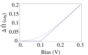
Figure 2: Example of the nonequilibrium noise spectrum at $T=0$ K (solid) and $300$ K (dashed) for a given phonon mode with frequency $\hbar\omega_{0}=0.1$ eV.

IV Numerical results for a simple two-level model

To build an intuitive understanding of the theory above, we now apply it to a simple spinless two-level model which could describe a diatomic molecule. For this model system, it is possible to do the calculation using the general results in Sec. III.1, without the approximations developed in Sec. III.3. We start from a model Hamiltonian for the isolated system,

$$H = H_{e}+H_{ph}+H_{int}$$ (77)

$$= \varepsilon_{0}(c^{\dagger}_{1}c_{1}-c^{\dagger}_{2}c_{2})-t(c^{\dagger}_{1}c_{2}+c^{\dagger}_{2}c_{1})$$

$$+ \sum_{i=1,2}\left(\frac{1}{2}\dot{u}_{i}^{2}+\frac{1}{2}\omega_{i}^{2}u_{i}^{2}+H^{i}_{int}\right).$$

The electrons couple with two phonon modes in the following two forms:

$$H^{1}_{int}=m_{1}u_{1}(c^{\dagger}_{1}c_{2}+c^{\dagger}_{2}c_{1}),$$ (78)

and

$$H^{2}_{int}=m_{2}u_{2}(c^{\dagger}_{1}c_{1}-c^{\dagger}_{2}c_{2}).$$ (79)

The first and second electronic levels couple with the left and right electrode, respectively, with level broadening $\Gamma$. A sketch of the model is shown in Fig. 3. Mode 1 corresponds to the bond-stretching mode of the diatomic molecule, while mode 2 mimics the rigid motion of the diatomic molecule between the two electrodes.

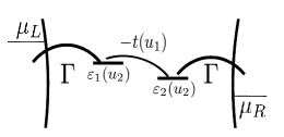
Figure 3: Schematic diagram of the two-level model. The bias is defined as $eV=\mu_{L}-\mu_{R}$ and the average electrochemical potential $\mu_{0}=(\mu_{L}+\mu_{R})/2$.

IV.1 Current-induced forces and phonon excitation

Figure 4 shows different parts of $\Lambda(\omega)$ and their Hilbert transforms. The solid and dashed lines in the bottom-right panel correspond to the NC and BP force. For the parameters used here, the NC and BP force are comparable with the diagonal RN and friction forces, shown in the two panels on top. The symmetry properties imply that the NC and the RN term become dominant in the limit of slow vibrations. The nonequilibrium RN term can be of interest, for example qualitatively changing the potential profileHussein et al. (2010); Nocera et al. (2011). Furthermore, by combining the RN term with a further contribution, arising from the next order in the expansion of the electronic Hamiltonian in powers of the displacements, it is possible to construct the full non-equilibrium dynamical response matrixDundas et al. (2012). Its bias-dependence can compete with the NC force and influence the appearance, or otherwise, of waterwheel modes.

In the present work the RN term only changes quantitatively the results for the model used. The RN term will be excluded altogether below, focusing instead on the effect of NC and BP force.

We already see from the analytical result that the magnitude of the BP force is directly related to the energy dependence of the electron spectrum. This is confirmed numerically in Figs. 5 and 6. We show in Fig. 5 the relative magnitude of the BP force compared with the average diagonal friction for different level broadenings $\Gamma$ at $1$ V with $\hbar\omega_{0}=0.02$ eV. The inset shows the left spectral function. We see that for a range of $\Gamma$, the BP force is of the same magnitude as the friction. With increasing $\Gamma$ the resonance in the DOS gets broader, and consequently the BP force gets smaller ($\propto\partial_{\varepsilon}R$ as in Eq. (69)). In Fig. 6 we vary the energy position of the bias window relative to the peak in the spectral function. The BP force drops quickly when the bias window moves away from the peak.

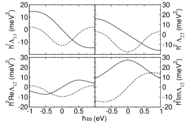
Figure 4: Different parts of the $\Lambda(\omega)$ function (solid) and their Hilbert transform (dashed). The model parameters are $\Gamma=1$ eV, $t=0.2$ eV, $\varepsilon_{0}=0$, $m_{1}=m_{2}=0.01$ eV/$\sqrt{{\rm amu}}$Å, $\mu_{0}=0$, and $V=1$ V. Indices 1 and 2 refer to the respective phonon modes. The equilibrium renormalization term has already been substracted in the plot. We use the same parameters in the following figures if not stated explicitly.

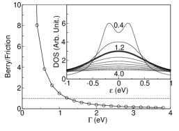
Figure 5: (main panel) Relative magnitude of the BP force compared with the average friction $2F_{BP}/({F_{FR}}_{11}+{F_{FR}}_{22})$ as a function of level broadening $\Gamma$ with $\hbar\omega_{0}=0.02$ eV. (inset) The electronic DOS function at different $\Gamma$. The BP force equals the friction at $\Gamma=1.2$ eV.

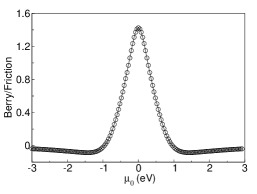
Figure 6: Relative magnitude of Berry force compared with the average friction felt by the two phonon modes ($({F_{FR}}_{11}+{F_{FR}}_{22})/2$) as a function of position of the average electrochemical potential $\mu_{0}$ at a bias of $1$ V.

Assuming a small detuning of the two harmonic oscillators $\hbar\omega_{\pm}=\hbar\omega_{0}\pm\delta/2$, we now study the bias dependence of their frequency, and damping described by their inverse Q-factors in Figs. 7 and 8. The runaway solution is defined at the point where the damping disappears, $1/Q_{i}=-2{\rm Im}\,\omega_{i}/{\rm Re}\,\omega_{i}=0$. We see that the BP force in general helps the runaway solution by reducing the threshold bias. This is prominent for larger detuning. The reason is that it bends the eigenmodes into ellipses so that the NC force continuously can take energy out of one mode, while pumping energy into the other. Eventually, this changes the polarization of the harmonic motion from linear to elliptical (circular) in mode space.

Comparing the full calculation with that from the wideband approximation, we see that they agree well only in the low bias regime. For large bias, we need to take into account the energy dependence of the electronic spectral function. The frequency dependence of the threshold bias with and without the BP force is depicted in Fig. 9. The divergent behavior of the threshold bias when only the NC force is considered is due to the finite range of the electron DOS (inset of Fig. 5). Once the bias is large enough for the bias window to enclose the DOS peaks, the NC force will saturate. Further increase of the bias does not help. But the BP force has an extra linear $\omega$ dependence (since it depends on $\dot{Q}$, instead of $Q$), which becomes important for high frequencies. The bias dependence of the mode-correlation function and derived excited phonon number (cf. Eq. (74)) corresponding to Figs. 7 is depicted in Fig. 10. Near the threshold bias, the sharp increase of the occupation number of one mode is a signature of the runaway solution. We will return to the signature in the Raman signal in Sec. VI.

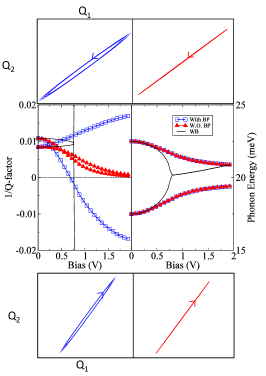
Figure 7: (Color online) The upper(lower) panels show the motion of positive(negative) damped branches calculated at $V=2$ V bias, with and without the BP force in left and right panels, respectively. The middle panel show the inverse Q-factor to the left, and the phonon energy as a function of bias to the right, with and without the BP force. The solid line is the result obtained from the wideband approximation, ignoring the BP force. Parameters used: $\hbar\omega_{0}=20$ meV, $\delta=5$ meV.

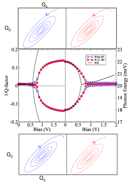
Figure 8: (Color online) The same as in Fig. 7, but now with $\delta=4$ meV.

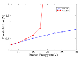
Figure 9: (Color online) The threshold bias as a function of phonon energy with or without BP force. The parameters are the same as in Fig. 7.

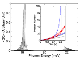
Figure 10: (Color online) Semi-classical displacement correlation function $\langle QQ\rangle$ of the two modes at different bias. The bias increases along the arrow shown. (inset) Excited phonon number as a function of bias. The dashed curves are the results when only the friction is included. The parameters are the same as in Fig. 7.

V Two extensions

V.1 Adiabatic limit

The perturbation approach we have presented, and illustrated with the model calculation above, is applicable to weak electron-phonon interaction. It is not restricted to slow ions. Within the same theoretical framework and based on the Hamiltonian in Eq. (6a)-Eq. (6c), we can carry out an adiabatic expansion, where the assumption is that the ions are moving slowly, while the electron-phonon interaction does not have to be smallBode et al. (2011, 2012).

In the limit of small ionic velocities, we expand the displacement in Eq. (II.2) at $\tau^{\prime}$ as follows,

$$X(\tau^{\prime})\approx Q({t})\sigma_{z}+\left(\dot{Q}(t)(t^{\prime}-t)\sigma_{z}+\frac{1}{2}\xi(t^{\prime})I_{2}\right),$$ (80)

where $\sigma_{z}$, $I_{2}$ are the Pauli and $2\times 2$ identity matrix, respectively. Using Eq. (80), we can re-group the expansion series in Eq. (II.2), and arrive at

$$G(\tau,\tau_{+})=\mathcal{G}_{0}(\tau,\tau_{+})+\sum_{k}\int_{K}\mathcal{G}_{0}(\tau,\tau^{\prime})M^{k}$$

$$\times\left(\dot{Q}_{k}({t})(t^{\prime}-t)\sigma_{z}+\frac{1}{2}\xi(t^{\prime})I_{2}\right)G(\tau^{\prime},\tau_{+})d\tau^{\prime}.$$ (81)

Now $\mathcal{G}_{0}(\tau,\tau_{+})\equiv\mathcal{G}_{0}(\tau,\tau_{+};Q(t))$ is the adiabatic electron Green’s function, determined by the instantaneous electronic Hamiltonian when the ions are at a given configuration ($Q(t)$).

The force due to the first term in the new Dyson equation now takes the same form as Eqs. (16-18), but the non-interacting electron spectral function $A_{\alpha}$ is replaced by the adiabatic one, $\mathcal{A}_{\alpha}(\varepsilon)\equiv\mathcal{A}_{\alpha}(\varepsilon;Q(t))$, which is upto infinite order in $M$,

$$\mathcal{F}^{(1)}_{k}=-2\sum_{\alpha}\int\frac{d\varepsilon}{2\pi}\;{{\rm Tr}}[\mathcal{A}_{\alpha}(\varepsilon)M^{k}]\Delta n^{\alpha}_{F}(\varepsilon).$$ (82)

Its contribution to the forces in the Langevin equation includes both the renormalization of the effective potential and the NC force. To see this, we assume $Q$ is small, and expand the adiabatic spectral function over $Q$ near $Q=0$. The first contribution ($Q=0$) is exactly the first order result of the perturbation calculation (Eq. (17)). The second contribution (linear in $Q$) can be split into a symmetric and an anti-symmetric part, which are the RN and NC force, respectively,

$$\frac{\partial\mathcal{F}^{(1)}}{\partial Q_{l}}$$

$$=-2\sum_{\alpha}\int\frac{d\varepsilon}{\pi}{\rm Re}{\rm Tr}\left[M^{k}\mathcal{G}_{0}^{r}(\varepsilon)M^{l}\mathcal{A}_{\alpha}(\varepsilon)\right]\Delta n_{F}^{\alpha}(\varepsilon)$$

$$=-2\sum_{\alpha}\int\frac{d\varepsilon}{\pi}{\rm Re}{\rm Tr}\left[M^{k}\mathcal{R}(\varepsilon)M^{l}\mathcal{A}_{\alpha}(\varepsilon)\right]\Delta n_{F}^{\alpha}(\varepsilon)$$

$$-2\sum_{\alpha}\int\frac{d\varepsilon}{2\pi}{\rm Im}{\rm Tr}\left[M^{k}\mathcal{A}(\varepsilon)M^{l}\mathcal{A}_{\alpha}(\varepsilon)\right]\Delta n_{F}^{\alpha}(\varepsilon).$$

We can see that in the limit $Q\to 0$ they agree with the $\omega\to 0$ limit of the perturbation results as we should expect. Note that above we have treated $M$ as $Q$-independent. If we relieve this assumption, then a further term enters the RN forceDundas et al. (2012).

The effective action from the second term in Eq. (81) is given by Eq. (19), with $Q_{l}(t^{\prime})\to\dot{Q}_{l}(t)(t^{\prime}-t)$, $A_{\alpha}(\varepsilon)\to\mathcal{A}_{\alpha}(\varepsilon)$. Its contributes to the Langevin equation in terms of the friction, the BP force, and the noise. To get the expressions for these forces, we need to (1) take the perturbation results in the $\omega\to 0$ limit, (2) replace $A_{\alpha}(\varepsilon)$ and $G_{0}^{r}(\varepsilon)$ with $\mathcal{A}_{\alpha}(\varepsilon)$ and $\mathcal{G}_{0}^{r}(\varepsilon)$, respectively. Again, the adiabatic results in the $Q\to 0$ limit agree with the perturbation results in the $\omega\to 0$ limit. We conclude this section with the diagram showing the relation between these two approximations (Fig. 11), and noting that the adiabatic approximation in principle allows for updating the parameters in the Hamiltonian along the path.

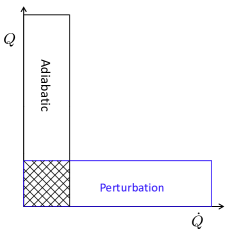
Figure 11: (Color online) The relation between the perturbation and the adiabatic expansion. The perturbation expansion assumes small deviation from the equilibrium configuration (small $Q$), while the adiabatic approximation assumes slow vibrations (small $\dot{Q}$). In the region where both $Q$ and $\dot{Q}$ are small, the two expansions agree with each other.

V.2 Coupling to electrode phonons

Actual molecular conductors are coupled also to electrode phonons. The energy dissipated by the electrons can be transferred to the electrodes via this additional channelLü and Wang (2007); Pecchia et al. (2007); Engelund et al. (2009); Tsutsui et al. (2008); Schulze et al. (2008). The effective action due to linear coupling with a bath of harmonic oscillators is well-knownFeynman and Vernon (1963); Caldeira and Leggett (1983); Schmid (1982). If we neglect the electron-phonon interaction in the electrodes, we can introduce the coupling to electrode-phonons in the Langevin equation Eq. (31) by adding the corresponding phonon self-energy: $\hat{\Pi}=\hat{\Pi}_{e}+\hat{\Pi}_{ph},\Pi^{r}=\Pi^{r}_{e}+\Pi^{r}_{ph}$. If the phonon baths are at equilibrium at a given temperature, they have two effects on the system. One is to modify the effective potential, and the other is to give rise to dissipation and fluctuating forces, which obey the fluctuation-dissipation theorem. It is straightforward to include a temperature difference between the two phonon baths. A Langevin equation including coupling only with phonon baths has been used in molecular dynamics simulations to study phonon heat transportDhar and Roy (2006); Wang (2007); Wang et al. (2009). It agrees with the Landauer formula in the low temperature limit, and with classical molecular dynamics in the high temperature limit.

It is possible to calculate the heat-flux between the central region and the phonon reservoirs in the electrodes using the self-energies describing these baths. If we connect the system to the two phonon baths ($L$ and $R$), and the nonequilibrium electron bath, then the retarded self-energy giving the deterministic force reads, $\Pi^{r}=\Pi^{r}_{e}+\Pi^{r}_{L}+\Pi^{r}_{R}$, and the fluctuating force is, $f=f_{L}+f_{R}+f_{e}$. When the system reaches a steady state, we can write,

$$\dot{H}_{ph}\equiv I_{e}+I_{L}+I_{R}\equiv 0,$$ (83)

where $I_{\alpha}$ is the energy current (power) flowing into the system from each bath, $\alpha$ ($\alpha=L,R,e$). Expressions for the power exchange can be found using the forces acting between the system and each bath in the Langevin equation,

$$I_{\alpha}(t)\equiv-\dot{Q}^{T}(t)\left(\int\Pi^{r}_{\alpha}(t-t^{\prime})Q(t^{\prime})dt^{\prime}-f_{\alpha}(t)\right).$$ (84)

Although we employ the harmonic approximation in this paper, this definition is valid also if there is anharmonic interaction inside the central regionWang (2007). This will be important for example when describing high-frequency molecular modes which only couple via anharmonic interaction to the low-frequency phonon modes in the electrodes. This situation can then be handled by a calculation where the surface parts of the electrodes are included explicitly in the definition of central region. We can write the expression for the energy current in frequency domain,

$$\bar{I}_{\alpha} \equiv \langle I_{\alpha}(t)\rangle$$

$$= -i\int\frac{d\omega}{2\pi}\omega\left({\rm tr}\left[\Pi^{r}_{\alpha}(\omega)\langle Q{Q}^{T}\rangle(\omega)-\langle f_{\alpha}Q^{T}\rangle(\omega)\right]\right)\,,$$

where ${\rm tr}$ denotes trace over phonon degrees of freedom in region $C$. Using the solution of the Langevin equation, and the noise correlation function, we can get a compact formula,

$$\bar{I}_{\alpha} = -i\int\frac{d\omega}{4\pi}\hbar\omega\,{\rm tr}\left[\tilde{\Pi}_{\alpha}(\omega)D^{r}(\omega)\hat{\Pi}(\omega)D^{a}(\omega)\right.$$ (86)

$$-\left.\hat{\Pi}_{\alpha}(\omega)D^{r}(\omega)\tilde{\Pi}(\omega)D^{a}(\omega)\right].$$

This result agrees with NEGF theoryLü and Wang (2007), and fullfills the energy conservation, e.g., $\sum_{\alpha=L,R,e}\bar{I}_{\alpha}=0$. Without the electron bath and anharmonic couplings, it reduces to the Landauer formula for phonon heat transportRego and Kirczenow (1998); Blencowe (1999); Mingo and Yang (2003); Mingo (2006); Yamamoto and Watanabe (2006); Wang et al. (2006). The formula contains information about the effects of the electrons and the electronic current on transport of heat to, from and across the central region, but these effects are beyond the scope of the present paper. Instead, we now focus on how the excitation of the localized vibrations by the current affects their Raman signals.

VI Raman spectroscopy and correlation functions

A central aspect of this work is that we need to find ways to actually observe the consequences of the current-induced forces. One promising routeIoffe et al. (2008); Ward et al. (2011) is the recent possibility of doing Raman spectroscopy on single, current-carrying molecules. In Raman spectroscopy one can deduce the “effective temperature” (or the degree of excitation) of the various Raman-active vibrational modes of a system. The semi-classical theory we have introduced is not applicable to Raman spectroscopy, since it always gives the same Stokes and anti-Stokes lines, for a reason that will be clear in the following. So we are forced to go back to the quantum-mechanical theory. Mathematically, the Raman spectrum can be written as follows,Schatz and Ratner (2002)

$$\mathscr{R}(\omega)=\int a_{k}\langle x_{k}(t)x_{l}(t^{\prime})\rangle a_{l}e^{i\omega(t-t^{\prime})}d(t-t^{\prime}).$$ (87)

Here $a_{k}$ is a vector involving the change in polarizability of the molecule when its atoms are displaced along the direction $k$ corresponding to the position operator $x_{k}$. When coupling with the electrode, $a_{k}$ could change due to interaction between the molecule and the electrodeOren et al. (2012). We will take it as a parameter, and focus on the displacement correlation function instead. Now $x_{k}(t)$ is an operator, and the average in Eq. (87) is a quantum-mechanical one. Since there is no time ordering in the quantum correlation function $\langle x_{k}(t)x_{l}(t^{\prime})\rangle$ at the heart of the Raman expression, it is best implemented in our path integral version with $t^{\prime}$ in the upper Keldysh contour and $t$ at the lower contour. Hence it can be represented as

$$\langle x_{k}(t)x_{l}(t^{\prime})\rangle = \mathcal{Z}^{-1}\int\mathcal{D}Q\int\mathcal{D}\xi\left(Q_{k}(t)-\frac{\xi_{k}(t)}{2}\right)$$ (88)

$$\times \left(Q_{l}(t^{\prime})+\frac{\xi_{l}(t^{\prime})}{2}\right)e^{\frac{i}{\hbar}S_{eff}(Q,\xi)},$$

where the effective action can be found in formula (19),

$$S_{eff}(Q,\xi) = -\frac{1}{2}\int\frac{d\omega}{2\pi}\left[Q^{\dagger}(\omega)L^{\dagger}(\omega)\xi(\omega)+\xi^{\dagger}(\omega)L(\omega)Q(\omega)\right.$$ (89)

$$\left.-i\xi^{\dagger}(\omega)\hat{\Pi}(\omega)\xi(\omega)\right],$$

and $\mathcal{Z}$ is a normalization factor. The Raman spectrum thus has four contributions. A classical contribution, $\mathscr{R}_{QQ}(\omega)$, proportional to the average of $Q_{k}(\omega)Q_{l}(\omega)^{*}$, two quantum corrections, $\mathscr{R}_{Q\xi}(\omega)$ and $\mathscr{R}_{\xi Q}(\omega)$, proportional to the averages of $Q_{k}(\omega)\xi_{l}(\omega)^{*}$ and $\xi_{k}(\omega)Q_{l}(\omega)^{*}$, and finally a contribution $\mathscr{R}_{\xi\xi}(\omega)$ proportional to $\xi_{k}(\omega)\xi_{l}(\omega)^{*}$. The calculation of these averages involves simple Gaussian integrals, and the results are

$$\mathscr{R}_{QQ}(\omega) = a_{k}[\hbar D^{r}(\omega)\hat{\Pi}(\omega)D^{a}(\omega)]_{kl}a_{l}$$ (90)

$$\mathscr{R}_{Q\xi}(\omega) = \frac{i}{2}a_{k}\hbar D^{r}_{kl}(\omega)a_{l}$$ (91)

$$\mathscr{R}_{\xi Q}(\omega) = -\frac{i}{2}a_{k}\hbar D^{a}_{kl}(\omega)a_{l}$$ (92)

$$\mathscr{R}_{\xi\xi}(\omega) = 0.$$ (93)

These functions are dominated by the properties close to the poles of $L^{-1}$. Let us first consider the case of one mode in thermal equilibrium. In this case $L(\omega)$ is a simple function which can be approximated as

$$L(\omega)=-\omega^{2}+\omega_{0}^{2}-i\eta\omega.$$ (94)

In the same approximation $\hat{\Pi}(\omega)$ is controlled by the fluctuation-dissipation theorem and becomes ($\beta=\hbar/(k_{B}T)$),

$$\hat{\Pi}(\omega)=\eta\omega\coth\left(\frac{\omega\beta}{2}\right).$$ (95)

The classical contribution is now

$$\mathscr{R}_{QQ}(\omega)=a^{2}\frac{\eta\hbar\omega\coth\left(\frac{\omega\beta}{2}\right)}{(-\omega^{2}+\omega_{0}^{2})^{2}+\eta^{2}\omega^{2}}.$$ (96)

This function yields a Raman signal which is symmetric in $\omega$. It has Lorentzian peaks at $\omega=\pm\omega_{0}$ of width $\eta/(2\omega_{0})$, and with strengths given by its area (integral over $\omega$), $a^{2}\hbar\pi/(2\omega_{0})\coth(\beta\omega_{0}/2)$. Note that the strength is proportional to temperature in the high-temperature limit. It is also important to note that the strength does not depend on the damping, $\eta$. The self-energy, $\hat{\Pi}(\omega)$, contributes a factor $\eta$ to the strength, but the $\omega$-integration contributes a factor $\eta^{-1}$, hence canceling the $\eta$ dependence. The physics of this is the fluctuation-dissipation theorem of equilibrium: a smaller damping should give higher oscillation amplitudes were it not for the associated decrease in fluctuations in the environment.

The quantum correction $\mathscr{R}_{Q\xi}(\omega)+\mathscr{R}_{\xi Q}(\omega)$ is proportional to the imaginary part of $L^{-1}$. In the above approximation it becomes,

$$\mathscr{R}_{Q\xi}(\omega)+\mathscr{R}_{\xi Q}(\omega)=a^{2}\frac{\eta\hbar\omega}{(-\omega^{2}+\omega_{0}^{2})^{2}+\eta^{2}\omega^{2}}.$$ (97)

This contribution breaks the $\omega\rightarrow-\omega$ symmetry, and is hence responsible for the different strengths of the Stokes(phonon emission) and anti-Stokes(phonon absorption) lines. This term also exhibits peaks at $\pm\omega_{0}$, with strengths $\pm a^{2}\hbar\pi/(2\omega_{0})$.

The ratio, $r$, of strengths of the anti-Stokes and Stokes lines becomes,

$$r=\frac{\coth\left(\frac{\beta\omega_{0}}{2}\right)-1}{\coth\left(\frac{\beta\omega_{0}}{2}\right)+1}=e^{-\beta\omega_{0}}.$$ (98)

In equilibrium this ratio is used to measure the temperature employing the particular mode excitation, but has also been used to estimate an effective temperature of the different modes out of equilibriumWard et al. (2007); Ioffe et al. (2008).

Next we discuss the situation in the presence of electronic current and the derived forces. We consider a situation with two modes close in frequency, which are coupled by the current. Now, the function $L(\omega)$ is a $2\times 2$ matrix. If the NC and BP forces are represented by constants, ${n}$ and ${b}$, respectively, then $L(\omega)$ becomes

$$L(\omega)=\left(\begin{array}[]{cc}-\omega^{2}+\omega_{1}^{2}-i\omega\eta&n-i\omega{b}\\ -{n}+i\omega{b}&-\omega^{2}+\omega_{2}^{2}-i\omega\eta\end{array}\right).$$ (99)

Here we have made the simplifying assumption that the friction, $\eta$, is the same for the two modes. The two mode frequencies $\omega_{1}$ and $\omega_{2}$ have a difference $\delta=\omega_{2}-\omega_{1}$. Comparing with the expressions Eqs. (67), (69), the parameters ${n}$ and ${b}$ are both linearly dependent on the applied voltage $V$. If this voltage is sufficiently large, there is a possibility that one of the eigenmodes of $L(\omega)$ will have a vanishing imaginary part at a critical voltage $V_{c}$, and we obtain a runaway mode.

In the following we present plots of the resulting Raman spectra as a function of voltage approaching $V_{c}$ from below. The function $\hat{\Pi}(\omega)$ describing the fluctuating forces is both temperature- and voltage-dependent. However, nothing dramatic happens at the critical voltage, so it will be taken to be a temperature and voltage independent matrix with values of the order of $\eta\omega$. As in the equilibrium case, an increasing lifetime of the mode will lead to stronger oscillation amplitudes, but out of equilibrium this need not be counteracted by decreasing fluctuations in the environment. The result is a strong increase in the strength of the runaway mode, both for the Stokes and the anti-Stokes line.

Figure 12 shows the Stokes lines for two modes close in frequency and coupled by the NC and BP forces, for the system described by Eq. (99). In the following graphs the parameters are, $\omega_{1}=\bar{\omega}-\delta/2$, $\omega_{2}=\bar{\omega}+\delta/2$ with $\delta=0.2\bar{\omega}$, $\eta=0.05\bar{\omega}$, ${b}/{n}=0.6/\bar{\omega}$, for which the critical value of the strength of the NC force will be ${n}_{c}=0.124\bar{\omega}^{2}$, when the voltage reaches its critical the value, $V_{c}$. We see that the mode at $\omega_{2}$ is increasing in strength while its frequency is shifting slightly down. By contrast the frequency of the mode at $\omega_{1}$ is moving upwards while the strength is decreasing. If we compare to the standard one-mode, equilibrium theory of Raman lines, we would say that one mode heats up, while the other cools down. This is seen clearly in Fig. 13, where the strength of the two modes is plotted as a function of voltage. Here we see a small cooling of one mode, while the other mode has a diverging temperature, as the voltage approaches $V_{c}$. Alternatively, one could use the ratio of the anti-Stokes/Stokes strengths in combination with Eq. (98) to determine an effective mode-temperature, as shown in Fig. 14. Interestingly, we cannot see the cooling effect from the anti-Stokes/Stokes ratio.

This could be qualitatively understood as follows. In principle, Eq. (88) only holds at equilibrium, which is a result of the fluctuation-dissipation theorem. Under nonequilibrium conditions, discrepancies between different ways of defining an effective temperature may be expected. Specifically, in the case studied here, the bias modifies the rates for phonon emission and absorption. This can be inferred from the change of peak broadening in the phonon correlation function, as well as from the shift of the peaks, with bias. Part of this bias-dependent effect is lost, when we form the anti-Stokes/Stokes ratio. But it is included when we look at the bias-dependent strength of the Stokes lines.

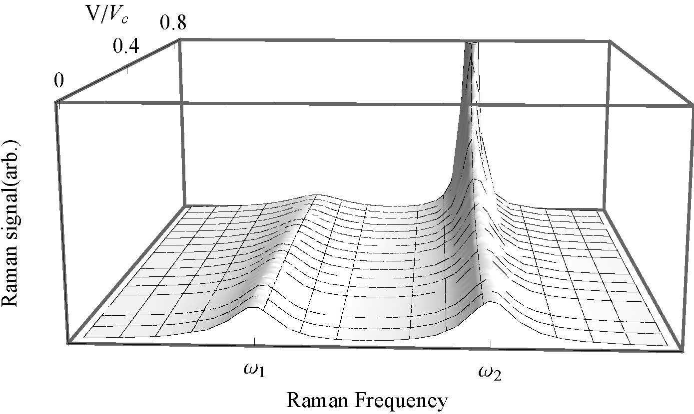
Figure 12: (Color online) The Stokes lines of two coupled modes for various values of the applied voltage in units of the critical voltage. Parameter values are $\omega_{1}=\bar{\omega}-\delta/2$, $\omega_{2}=\bar{\omega}+\delta/2$ with $\delta=0.2\bar{\omega}$, $\eta=0.05\bar{\omega}$, ${b}/{n}=0.6/\bar{\omega}$.

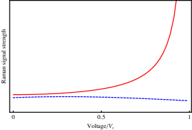
Figure 13: (Color online) Strength of the two Stokes lines as a function of voltage. Solid line corresponds to the “runaway” mode at $\omega_{2}$, and dashed line to the “cooling” mode at $\omega_{1}$.

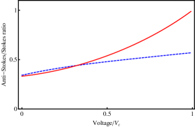
Figure 14: (Color online) Ratio of strengths of the anti-Stokes and Stokes lines as a function of voltage. Parameters are as in Fig. 12. Solid line corresponds to the “runaway” mode at $\omega_{2}$, and dashed line to the “cooling” mode at $\omega_{1}$.

VII Concluding remarks

In this paper we have derived a semi-classical Langevin equation describing the motion of the ions, in the harmonic approximation, in nanoscale conductors including both the effective action from the current-carrying electrons and the coupling to the phonon baths in the electrodes. Joule heating and current-induced forces are described on an equal footing by this methodology. We derive a convergent expression for the BP force, removing the infrared divergence in our previous resultLü et al. (2010). The importance of the BP force in relation to the stability of the device is further highlighted in a two-level model system. Using the same model we show the signature of the current-induced runaway mode excitation in the Raman spectroscopy of a current-carrying molecular conductorIoffe et al. (2008); Ward et al. (2011).

We should mention that the harmonic approximation used here breaks down when the phonons are highly excited. In that case the anharmonic coupling between different phonon modes becomes important. Analysis in this regime relies e.g. on molecular dynamics simulation. To take the nonlinear potential approximately into account in the present method, we only need to replace the force from the harmonic potential $-KQ(t)$ with the full potential $-\partial_{Q}V(Q)$. Thus the full Langevin equation has the following advantages: first, we can include the highly nonlinear ion potential, which is necessary to simulate bond-breaking processes; second, a crucial part of the quantum-mechanical motion is included in the dynamics. For example, we recover the quantum-mechanical results for Joule heating and for heat transport in the harmonic limit. This enables the study of phonon heat transportWang et al. (2008), or thermoelectricDubi and Di Ventra (2011) transport using the same Langevin equation including the electron-phonon interaction, and is an interesting topic for future research.

The backaction of the runaway vibrations on the electrons is another possible extension of the present study. There are at least two effects to address. The first one is the adiabatic change of the electronic structure. The purpose of the adiabatic extension in Sec. V.1 is to include this effect. The second effect is the inelastic electrical current, which becomes important when the electron mean free path is comparable to the device length.

A number of problems need to be faced when implementing the approach within the framework of density functional theory. First, the ions may be driven away from their equilibrium positions by the current. The electronic structure and electron-phonon coupling depend on the ionic positions, and one may need to update the electronic friction and noise correlation function throughout the molecular dynamics simulation. This introduces a technical problem, in addition to the computational challenge, which is how to generate colored noise when its correlation function is time-dependent. Second, calculation of the convolution kernel in the Langevin equation is time-consuming considering the many time-steps needed to sample the dynamics. For the electron bath in the wideband limit the convolution transforms to time-local forces. But the time-scale of the phonon bath is typically comparable to that of the system, and we cannot use the wideband approximation. One possible solution could be to include more ions from the baths into the dynamical region and approximate the coupling to the external phonon bath with time-local forces. Intuitively, with more ions included, the approximate central system will be closer to the actual system under study. Work to overcome these difficulties is underway.

Electron-nuclear dynamics is a broad problem, relevant to many fields. A central challenge is how to take account of electron-nuclear correlation. The simplest form of nonadiabatic dynamics - the Ehrenfest approximation - fails precisely there: it does not take into account spontaneous phonon emission by excited electrons and consequently the Joule heating effect. The appeal of Ehrenfest dynamics is its conceptual simplicity derived from the classical treatment of the nuclei. The Langevin approach retains this key element, while rigorously reinstating the vital missing ingredient: the fluctuating forces - with the correct noise spectrum - exerted by the electron gas and responsible for the return of energy from excited electrons to thermal vibrations. Thus, in addition to its capabilities as a method for nonadiabatic dynamics, this approach can be very helpful conceptually, by explicitly quantifying effects that are intuitive but whose physical content can sometimes remain hidden from view.

Although our discussion here is in the context of molecular electronics, we believe that the predictions based on the simple model can be important for other interesting physical systems, for instance nano-electromechanical oscillators (NEMS) coupling with an atomic point contactKemiktarak et al. (2007); Poggio et al. (2008). When the current through an atomic point contact is used to measure the motion of an oscillator, the measurement imposes quantum backaction on the oscillator. A similar Hamiltonian describes this quantum backaction quite wellHussein et al. (2010); Bennett et al. (2010); Nocera et al. (2011). If we now couple two identical oscillators, or two nearly-degenerate eigenmodes by the point contact, it seems to be experimentally feasible to detect the polarized motion predicted herePerisanu et al. (2010); Karabalin et al. (2011).

A neighbouring field, where much larger size- and time-scales come into play, and where Langevin dynamics is an important line of approach, is the simulation of radiation damageRace et al. (2010). It is hoped that the present discussion will be of interest to that community.

Appendix A Connection with Nano Lett., 10, 1657 (2010)

In Ref. Lü et al., 2010, we carried out an adiabatic expansion in a slightly different way from that in Sec. V.1. We obtained an infrared divergence in the expression for the BP force, and used the largest phonon frequency as a cutoff. Here we show that by introducing a small lifetime broadening to the scattering eigenstate ($\gamma$), we can remove the divergence, and get the same result as shown in this paper. We start from the expression for the Berry force in Ref. Lü et al., 2010, and write it as

$$\mathcal{B}=-\lim_{\gamma\to 0}\int d\omega\frac{{\rm Im}\Delta\Lambda(\omega)}{(\omega-i\gamma)^{2}}.$$ (100)

We first do a partial integration to get

$$\mathcal{B}=-\lim_{\gamma\to 0}\int\frac{d\omega}{\omega-i\gamma}\partial_{\omega}{\rm Im}\Delta\Lambda(\omega).$$ (101)

From the $\omega$-dependent part of ${\rm Im}\Delta\Lambda(\omega)$(Eq. (50))

$$\lim_{\gamma\to 0}{\rm}\int d\omega\frac{\partial_{\omega}\mathcal{A}(\varepsilon_{+})+\partial_{\omega}\mathcal{A}(\varepsilon_{-})}{\omega-i\gamma}\sim-4\pi\hbar\partial_{\varepsilon}{\cal R}(\varepsilon),$$

which gives

$$\mathcal{B} \approx 2\hbar\sum_{\alpha}\int\frac{d\varepsilon}{\pi}\;\Delta n_{F}^{\alpha}(\varepsilon)$$ (103)

$$\times {{\rm Im}{\rm Tr}}[M\mathcal{A}_{\alpha}(\varepsilon)M\partial_{\varepsilon}{\rm Re}{\cal R}(\varepsilon)].$$

This agrees with the result in Sec. V.1.

In the wideband limit, ignoring the $\omega$ dependence of ${\rm Im}\Delta\Lambda$, we get

$$\mathcal{B}\approx\frac{2\hbar eV}{\pi\Omega_{c}}\chi^{-},$$ (104)

where $\Omega_{c}$ is an upper bound on the electron-hole pair excitation. In Ref. Lü et al., 2010, we used the largest phonon frequency instead, which over-estimates the effect of BP force. If as a conservative estimate of $\Omega_{c}$ we take a typical hopping matrix element, then using $\dot{Q}/Q\sim\omega$ we get the estimate in (64).

Appendix B Alternative derivation of the Langevin equation

In this Appendix, we give an alternative way of arriving at the generalized Langevin equation (Eq. (31)). The derivation here is meant to be intuitive rather than theoretically rigorous. Our starting point is the equation of motion for the (mass-normalised) displacement operator $u$,

$$\ddot{x}=-Kx+F_{e},$$ (105)

where we define the electronic force operator

$$F_{e}=-\frac{\partial H_{e}(x)}{\partial x}.$$ (106)

With the help of Green’s functions, Eq. (105) can be cast into the following form, for each degree of freedom $k$,

$$\ddot{x}_{k} = -\sum_{j}K_{kj}x_{j}+i\hbar{\rm Tr}\left[M^{k}G^{<}(t,t_{+})\right]+{f}_{k}(t).$$ (107)

We have defined the noise operator

$${f}_{k}(t)=i\sum_{m,n}M_{mn}^{k}\left(ic_{m}^{\dagger}(t)c_{n}(t)-\hbar G^{<}_{nm}(t,t_{+})\right),$$ (108)

and the lesser Green’s function is $G_{nm}^{<}(t,t_{+})=(i/\hbar)\langle c^{\dagger}_{m}(t_{+})c_{n}(t)\rangle$. The quantum average $\langle\dots\rangle$ is over the electronic environment, which need not be in equilibrium.

From Eq. (II.2) to second order in $M$,

$$G^{<}(t,t_{+})=G^{<}_{0}(t,t_{+})$$

$$+ \sum_{k}\int G_{0}(t,t^{\prime})M^{k}x_{k}(t^{\prime})G_{0}^{<}(t^{\prime},t_{+})dt^{\prime}$$

$$- \sum_{k}\int G_{0}^{<}(t,t^{\prime})M^{k}x_{k}(t^{\prime})\bar{G}_{0}(t^{\prime},t_{+})dt^{\prime}.$$

Using this in Eq. (107), we get

$$\ddot{x}_{k} = -\sum_{j}K_{kj}x_{j}+i\hbar{\textrm{Tr}}[M^{k}G^{<}_{0}(t,t_{+})]$$ (110)

$$-\sum_{j}\int\Pi^{r}_{kj}(t,t^{\prime})x_{j}(t^{\prime})dt^{\prime}+{f}_{k}(t),$$

which is of the same form as Eq. (31).

Now consider the time correlation of the noise operator $f$,

$$\langle f_{i}(t)f_{j}(t^{\prime})\rangle = \hbar^{2}{\textrm{Tr}}[M^{i}G_{0}^{>}(t,t^{\prime})M^{j}G_{0}^{<}(t^{\prime},t)]$$ (111)

$$= i\hbar\Pi^{>}_{ij}(t,t^{\prime})\,,$$

and

$$\langle f_{j}(t^{\prime})f_{i}(t)\rangle=i\hbar\Pi^{<}_{ij}(t,t^{\prime})\,.$$ (112)

As expected, the quantum-mechanical noise operators at different times does not commute.

To go to the semi-classical approximation, we take the classical noise correlation as the average of Eqs. (111) and (112),

$$\langle f_{i}(t)f_{j}(t^{\prime})\rangle_{c}=\langle f_{j}(t^{\prime})f_{i}(t)\rangle_{c}$$

$$= \frac{1}{2}(\langle f_{i}(t)f_{j}(t^{\prime})\rangle+\langle f_{j}(t^{\prime})f_{i}(t)\rangle),$$

where $\langle\dots\rangle_{c}$ denotes a classical statistical average. Now the noise spectrum becomes “classical”, in the sense that its time correlation function is real. If the potential is anharmonic, the right side of Eq. (110) will contain terms of higher order in $u$. The equations of motion of these higher-order terms form an infinite hierarchy. Then the semi-classical approximation will have to involve a truncation procedure. However, this is a separate problem, beyond the scope of this paper.

We stress again that after making the semi-classical approximation, it is still possible to calculate the quantum-mechanical average of two displacement operators at equal times $\langle u_{i}(t)u_{j}(t)\rangle$ within the harmonic approximation, from the semi-classical Langevin equation, leading to the correct quantum-mechanical vibrational energy and steady-state transport properties.

Appendix C The phonon self-energy

The phonon self-energies correspond to the bubble diagram in Fig. 1:

$$\Pi^{<,>}_{kl}(t-t^{\prime}) = -i\hbar\,{\rm Tr}\left[M^{k}G^{<,>}_{0}(t-t^{\prime})M^{l}G^{>,<}_{0}(t^{\prime}-t)\right],$$

$$\Pi^{r,a}_{kl}(t-t^{\prime}) = -i\hbar\,{\rm Tr}\left[M^{k}G^{r,a}_{0}(t-t^{\prime})M^{l}G^{<}_{0}(t^{\prime}-t)\right]$$ (114)

$$-i\hbar\,{\rm Tr}\left[M^{k}G^{<}_{0}(t-t^{\prime})M^{l}G^{a,r}_{0}(t^{\prime}-t)\right].$$

References

- Reed et al. (1997) M. A. Reed, C. Zhou, C. J. Muller, T. P. Burgin, and J. M. Tour, Science 278, 252 (1997).
- Smit et al. (2002) R. H. M. Smit, Y. Noat, C. Untiedt, N. D. Lang, M. C. van Hemert, and J. M. van Ruitenbeek, Nature 419, 906 (2002).
- Rubio et al. (1996) G. Rubio, N. Agraït, and S. Vieira, Phys. Rev. Lett. 76, 2302 (1996).
- Yanson et al. (1998) A. I. Yanson, G. R. Bollinger, H. E. van den Brom, N. Agraït, and J. M. van Ruitenbeek, Nature 395, 783 (1998).
- Ohnishi et al. (1998) H. Ohnishi, Y. Kondo, and K. Takayanagi, Nature 395, 780 (1998).
- Pascual et al. (2003) J. I. Pascual, N. Lorente, Z. Song, H. Conrad, and H. P. Rust, Nature 423, 525 (2003).
- Tao (2006) N. J. Tao, Nature Nanotech. 1, 173 (2006).
- Lindsay and Ratner (2007) S. M. Lindsay and M. A. Ratner, Advanced Materials 19, 23 (2007).
- Galperin et al. (2008) M. Galperin, M. A. Ratner, A. Nitzan, and A. Troisi, Science 319, 1056 (2008).
- Schulze et al. (2008) G. Schulze, K. J. Franke, A. Gagliardi, G. Romano, C. S. Lin, A. L. Rosa, T. A. Niehaus, T. Frauenheim, A. Di Carlo, A. Pecchia, et al., Phys. Rev. Lett. 100, 136801 (2008).
- Galperin et al. (2007) M. Galperin, M. A. Ratner, and A. Nitzan, J. Phys.:Condens. Matter 19, 103201 (2007).
- Horsfield et al. (2006) A. P. Horsfield, D. R. Bowler, H. Ness, C. G. Sánchez, T. N. Todorov, and A. J. Fisher, Rep. Prog. Phys. 69, 1195 (2006).
- Stipe et al. (1998) B. C. Stipe, M. A. Rezaei, and W. Ho, Science 280, 1732 (1998).
- Agraït et al. (2003) N. Agraït, A. L. Yeyati, and J. M. van Ruitenbeek, Phys. Rep. 377, 81 (2003).
- Agraït et al. (2002) N. Agraït, C. Untiedt, G. Rubio-Bollinger, and S. Vieira, Phys. Rev. Lett. 88, 216803 (2002).
- Park et al. (2000) H. Park, J. Park, A. K. L. Lim, E. H. Anderson, A. P. Alivisatos, and P. L. McEuen, Nature 407, 57 (2000).
- Viljas et al. (2005) J. K. Viljas, J. C. Cuevas, F. Pauly, and M. Häfner, Phys. Rev. B 72, 245415 (2005).
- Frederiksen et al. (2004) T. Frederiksen, M. Brandbyge, N. Lorente, and A.-P. Jauho, Phys. Rev. Lett. 93, 256601 (2004).
- Paulsson et al. (2005) M. Paulsson, T. Frederiksen, and M. Brandbyge, Phys. Rev. B 72, 201101 (2005).
- Frederiksen et al. (2007) T. Frederiksen, M. Paulsson, M. Brandbyge, and A.-P. Jauho, Phys. Rev. B 75, 205413 (2007).
- Paulsson et al. (2008) M. Paulsson, T. Frederiksen, H. Ueba, N. Lorente, and M. Brandbyge, Phys. Rev. Lett. 100, 226604 (2008).
- Sergueev et al. (2005) N. Sergueev, D. Roubtsov, and H. Guo, Phys. Rev. Lett. 95, 146803 (2005).
- Pecchia et al. (2007) A. Pecchia, G. Romano, and A. Di Carlo, Phys. Rev. B 75, 035401 (2007).
- McEniry et al. (2007) E. J. McEniry, D. R. Bowler, D. Dundas, A. P. Horsfield, C. G. Sanchez, and T. N. Todorov, J. Phys.:Condens. Matter 19, 196201 (2007).
- Chen et al. (2003) Y.-C. Chen, M. Zwolak, and M. Di Ventra, Nano Lett. 3, 1691 (2003).
- Todorov (1998) T. N. Todorov, Philos. Mag. B 77, 965 (1998).
- Segal and Nitzan (2002) D. Segal and A. Nitzan, J. Chem. Phys. 117, 3915 (2002).
- Huang et al. (2007) Z. Huang, F. Chen, R. D’Agosta, P. A. Bennett, M. Di Ventra, and N. J. Tao, Nature Nanotech. 2, 698 (2007).
- Ness et al. (2001) H. Ness, S. A. Shevlin, and A. J. Fisher, Phys. Rev. B 63, 125422 (2001).
- Braig and Flensberg (2003) S. Braig and K. Flensberg, Phys. Rev. B 68, 205324 (2003).
- Mitra et al. (2004) A. Mitra, I. Aleiner, and A. J. Millis, Phys. Rev. B 69, 245302 (2004).
- Härtle et al. (2009) R. Härtle, C. Benesch, and M. Thoss, Phys. Rev. Lett. 102, 146801 (2009).
- Lorente et al. (2001) N. Lorente, M. Persson, L. J. Lauhon, and W. Ho, Phys. Rev. Lett. 86, 2593 (2001).
- Mii et al. (2003) T. Mii, S. G. Tikhodeev, and H. Ueba, Phys. Rev. B 68, 205406 (2003).
- Asai (2008) Y. Asai, Phys. Rev. B 78, 045434 (2008).
- Lü and Wang (2007) J. T. Lü and J.-S. Wang, Phys. Rev. B 76, 165418 (2007).
- Jiang et al. (2005) J. Jiang, M. Kula, W. Lu, and Y. Luo, Nano Lett. 5, 1551 (2005).
- Kushmerick et al. (2004) J. G. Kushmerick, J. Lazorcik, C. Patterson, R. Shashidhar, D. Seferos, and G. Bazan, Nano Lett. 4, 639 (2004).
- Galperin et al. (2006) M. Galperin, A. Nitzan, and M. Ratner, Phys. Rev. B 73, 045314 (2006).
- Tsutsui et al. (2008) M. Tsutsui, M. Taniguchi, and T. Kawai, Nano Lett. 8, 3293 (2008).
- Verdozzi et al. (2006) C. Verdozzi, G. Stefanucci, and C. Almbladh, Phys. Rev. Lett. 97, 046603 (2006).
- Hihath et al. (2008) J. Hihath, C. R. Arroyo, G. Rubio-Bollinger, N. J. Tao, and N. Agraït, Nano Lett. 8, 1673 (2008).
- Smit et al. (2004) R. H. M. Smit, C. Untiedt, and van Ruitenbeek J. M., Nanotechnology 15, S472 (2004).
- Tsutsui et al. (2006) M. Tsutsui, S. Kurokawa, and A. Sakai, Nanotechnology 17, 5334 (2006).
- Stamenova et al. (2006) M. Stamenova, S. Sahoo, C. G. Sánchez, T. N. Todorov, and S. Sanvito, Phys. Rev. B 73, 094439 (2006).
- Zhang et al. (2011) R. Zhang, I. Rungger, S. Sanvito, and S. Hou, Phys. Rev. B 84, 085445 (2011).
- Jorn and Seideman (2009) R. Jorn and T. Seideman, J. Chem. Phys. 131, 244114 (2009).
- Jorn and Seideman (2010) R. Jorn and T. Seideman, Acc. Chem. Res. 43, 1186 (2010).
- Okabayashi et al. (2010) N. Okabayashi, M. Paulsson, H. Ueba, Y. Konda, and T. Komeda, Phys. Rev. Lett. 104, 077801 (2010).
- Fock et al. (2011) J. Fock, J. K. Sørensen, E. Lörtscher, T. Vosch, C. A. Martin, H. Riel, K. Kilså, T. Bjørnholm, and H. v. d. Zant, Phys. Chem. Chem. Phys. 13, 14325 (2011).
- Kim et al. (2011) Y. Kim, T. Pietsch, A. Erbe, W. Belzig, and E. Scheer, Nano Letters 11, 3734 (2011).
- Sorbello (1998) R. S. Sorbello, Solid State Physics 51, 159 (1998).
- Dundas et al. (2009) D. Dundas, E. J. McEniry, and T. N. Todorov, Nature Nanotech. 4, 99 (2009).
- Todorov et al. (2010) T. N. Todorov, D. Dundas, and E. J. McEniry, Phys. Rev. B 81, 075416 (2010).
- Lü et al. (2010) J. T. Lü, M. Brandbyge, and P. Hedegård, Nano Lett. 10, 1657 (2010).
- Todorov et al. (2011) T. N. Todorov, D. Dundas, A. T. Paxton, and A. P. Horsfield, Beilstein J. Nanotechnol. 2, 727 (2011).
- Lü et al. (2011a) J. T. Lü, T. Gunst, M. Brandbyge, and P. Hedegård, Beilstein J. Nanotechnol. 2, 814 (2011a).
- Bode et al. (2011) N. Bode, S. V. Kusminskiy, R. Egger, and F. von Oppen, Phys. Rev. Lett. 107, 036804 (2011).
- Bode et al. (2012) N. Bode, S. V. Kusminskiy, R. Egger, and F. von Oppen, Beilstein J. Nanotechnol. 3, 144 (2012).
- Dzhioev and Kosov (2011) A. A. Dzhioev and D. S. Kosov, J. Chem. Phys. 135, 074701 (2011).
- Nocera et al. (2011) A. Nocera, C. A. Perroni, V. Marigliano Ramaglia, and V. Cataudella, Phys. Rev. B 83, 115420 (2011).
- Head-Gordon and Tully (1995) M. Head-Gordon and J. Tully, J. Chem. Phys. 103, 10137 (1995).
- Lü et al. (2011b) J. T. Lü, P. Hedegård, and M. Brandbyge, Phys. Rev. Lett. 107, 046801 (2011b).
- Brandbyge and Hedegård (1994) M. Brandbyge and P. Hedegård, Phys. Rev. Lett. 72, 2919 (1994).
- Brandbyge et al. (1995) M. Brandbyge, P. Hedegård, T. F. Heinz, J. A. Misewich, and D. M. Newns, Phys. Rev. B 52, 6042 (1995).
- Mozyrsky et al. (2006) D. Mozyrsky, M. B. Hastings, and I. Martin, Phys. Rev. B 73, 035104 (2006).
- Hussein et al. (2010) R. Hussein, A. Metelmann, P. Zedler, and T. Brandes, Phys. Rev. B 82, 165406 (2010).
- Metelmann and Brandes (2011) A. Metelmann and T. Brandes, Phys. Rev. B 84, 155455 (2011).
- Feynman and Vernon (1963) R. P. Feynman and F. L. Vernon, Ann. Phys. 24, 118 (1963).
- Caldeira and Leggett (1983) A. Caldeira and A. Leggett, Physica A 121, 587 (1983).
- Schmid (1982) A. Schmid, J. Low Temp. Phys. 49, 609 (1982).
- Mahan (1990) G. D. Mahan, Many-Particle Physics (Plenum Press, 1990).
- Haug and Jauho (2008) H. Haug and A.-P. Jauho, Quantum Kinetics in Transport and Optics of Semiconductors (Springer, New York, 2008).
- Brandbyge et al. (2003) M. Brandbyge, K. Stokbro, J. Taylor, J. L. Mozos, and P. Ordejon, Phys. Rev. B 67, 193104 (2003).
- Bevan et al. (2010) K. H. Bevan, H. Guo, E. D. Williams, and Z. Zhang, Phys. Rev. B 81, 235416 (2010).
- McEniry et al. (2008) E. J. McEniry, T. Frederiksen, T. N. Todorov, D. Dundas, and A. P. Horsfield, Phys. Rev. B 78, 035446 (2008).
- McEniry et al. (2009) E. J. McEniry, T. N. Todorov, and D. Dundas, J. Phys.: Condens. Matter 21, 195304 (2009).
- Dundas et al. (2012) D. Dundas, B. Cunningham, C. Buchanan, A. Terasawa, A. P. Paxton, and T. N. Todorov, submitted (2012).
- Engelund et al. (2009) M. Engelund, M. Brandbyge, and A. P. Jauho, Phys. Rev. B 80, 045427 (2009).
- Dhar and Roy (2006) A. Dhar and D. Roy, J. Stat. Phys. 125, 801 (2006).
- Wang (2007) J.-S. Wang, Phys. Rev. Lett. 99, 160601 (2007).
- Wang et al. (2009) J.-S. Wang, X. Ni, and J.-W. Jiang, Phys. Rev. B 80, 224302 (2009).
- Rego and Kirczenow (1998) L. G. C. Rego and G. Kirczenow, Phys. Rev. Lett. 81, 232 (1998).
- Blencowe (1999) M. P. Blencowe, Phys. Rev. B 59, 4992 (1999).
- Mingo and Yang (2003) N. Mingo and L. Yang, Phys. Rev. B 68, 245406 (2003).
- Mingo (2006) N. Mingo, Phys. Rev. B 74, 125402 (2006).
- Yamamoto and Watanabe (2006) T. Yamamoto and K. Watanabe, Phys. Rev. Lett. 96, 255503 (2006).
- Wang et al. (2006) J.-S. Wang, J. Wang, and N. Zeng, Phys. Rev. B 74, 033408 (2006).
- Ioffe et al. (2008) Z. Ioffe, T. Shamai, A. Ophir, G. Noy, I. Yutsis, K. Kfir, O. Cheshnovsky, and Y. Selzer, Nature Nanotech. 3, 727 (2008).
- Ward et al. (2011) D. R. Ward, D. A. Corley, J. M. Tour, and D. Natelson, Nature Nanotech. 6, 33 (2011).
- Schatz and Ratner (2002) G. C. Schatz and M. A. Ratner, Quantum mechanics in Chemistry (Dover, New York, 2002).
- Oren et al. (2012) M. Oren, M. Galperin, and A. Nitzan, Phys. Rev. B 85, 115435 (2012).
- Ward et al. (2007) D. R. Ward, N. K. Grady, C. S. Levin, N. J. Halas, Y. Wu, P. Nordlander, and D. Natelson, Nano Lett. 7, 1396 (2007).
- Wang et al. (2008) J.-S. Wang, J. Wang, and J. T. Lü, Euro. Phys. J. B 62, 381 (2008).
- Dubi and Di Ventra (2011) Y. Dubi and M. Di Ventra, Rev. Mod. Phys. 83, 131 (2011).
- Kemiktarak et al. (2007) U. Kemiktarak, T. Ndukum, K. C. Schwab, and K. L. Ekinci, Nature 450, 85 (2007).
- Poggio et al. (2008) M. Poggio, M. P. Jura, C. L. Degen, M. A. Topinka, H. J. Mamin, D. Goldhaber-Gordon, and D. Rugar, Nature Phys. 4, 635 (2008).
- Bennett et al. (2010) S. D. Bennett, J. Maassen, and A. A. Clerk, Phys. Rev. Lett. 105, 217206 (2010).
- Perisanu et al. (2010) S. Perisanu, T. Barois, A. Ayari, P. Poncharal, M. Choueib, S. T. Purcell, and P. Vincent, Phys. Rev. B 81, 165440 (2010).
- Karabalin et al. (2011) R. B. Karabalin, R. Lifshitz, M. C. Cross, M. H. Matheny, S. C. Masmanidis, and M. L. Roukes, Phys. Rev. Lett. 106, 094102 (2011).
- Race et al. (2010) C. P. Race, D. R. Mason, M. W. Finnis, W. M. C. Foulkes, A. P. Horsfield, and A. P. Sutton, Rep. Prog. Phys. 73, 116501 (2010).