Intrinsic Spin-Orbit Interaction in Graphene

Abstract

In graphene, we report the first theoretical demonstration of how the intrinsic spin orbit interaction can be deduced from the theory and how it can be controlled by tuning a uniform magnetic field, and/or by changing the strength of a long range Coulomb like impurity (adatom), as well as gap parameter. In the impurity context, we find that intrinsic spin-orbit interaction energy may be enhanced by increasing the strength of magnetic field and/or by decreasing the band gap mass term. Additionally, it may be strongly enhanced by increasing the impurity strength. Furthermore, from the proposal of Kane and Mele [Phys. Rev. Lett. 95, 226801 (2005)], it was discussed that the pristine graphene has a quantized spin Hall effect regime where the Rashba type spin orbit interaction term is smaller than that of intrinsic one. Our analysis suggest the nonexistence of such a regime in the ground state of flat graphene.

The spin-orbit effect is purely kinematic effect, and arises due to the interaction of the orbital and spin internal degrees of freedom. Recently, there has been growing interest in the study of this effect in graphene, due the fact that the progress in manipulating grapheneNOVOSELOV2004 , and graphene based nanostructures, particularly graphene quantum dots CHEN2007 ; RYCERZ2007 ; BADARSON2009 has opened new perspectives in usage of spin qubits LOSS1998 for quantum computing and quantum information purposes RECHER2010 . Graphene based nanostructures seem to be proper candidate for realizing these kind of processes through controlling one or two basic spin interactions such as intrinsic or Rashba type spin-orbit interactions (SOIs) KANE2005 ; HARNENDO2006 ; MIN2006 ; KUEMMETH2008 ; RASHBA2009 ; HARNENDO2009 ; NETO2009 ; GMITRA2009 ; RAKYTA2010 ; SANCHO2011 ; ABANIN2011 ; BLIOKH2011 ; LIU2012 . Since the former is supposed to be small, investigations are focused on the latter one which assigns a finite mass for the graphene carriers due to the interaction with substrate, and thus leading to a finite gap. In fact, within the Spin Quantum Hall Effect (SQHE) context, investigations were initiated by Kane and Mele’s workKANE2005 . They proposed that the ground state of graphene exhibits a SQHE. They showed that SQHE regime exists provided that Rashba type SOI term, $\Delta_{\mathrm{SO}}^{\mathrm{R}}\sim 0.05\ \mathrm{meV}$, smaller than that found for intrinsic SOI, $\Delta_{\mathrm{SO}}^{\mathrm{I}}\sim 0.103\ \mathrm{meV}$. Later, on the basis of microscopic considerations, $\Delta_{\mathrm{SO}}^{\mathrm{I}}(\Delta_{\mathrm{SO}}^{\mathrm{R}})$ is estimated to be much smaller (larger) than that of found by Kane and Mele: For instance, Hernando et alHARNENDO2009 found $\Delta_{\mathrm{SO}}^{\mathrm{I}}\sim 0.86\ \mu\mathrm{eV}$, Min et alMIN2006 found $\Delta_{\mathrm{SO}}^{\mathrm{I}}\sim 0.57\ \mu\mathrm{eV}$, $\Delta_{\mathrm{SO}}^{\mathrm{R}}\sim 0.011\ \mathrm{meV}$. Nevertheless, it is concluded that SQHE regime can occur only below a temperature $\Delta_{\mathrm{SO}}^{\mathrm{I}}\sim 0.01\ K$ ($10^{-3}\ \mathrm{meV}$). In the impurity context, very recently Castro and NetoNETO2009 showed that impurity induced distortion in flat graphene lead to a significant enhancement of SOI about $\Delta_{\mathrm{SO}}^{\mathrm{IMP}}\sim 1-7\ \mathrm{meV}$. While our analysis confirms this estimate within the pure impurity coverage, but it reveals that, in the absence of impurities, i.e., in the case of flat graphene, there is no experimentally accessible temperature where SQHE regime can occur.

Since intrinsic SOI is a natural property of Dirac’s equation, i.e., it inherently involves the spin degrees of freedom, its Graphene’s analog contains pseudospin or just spin-orbit interaction automatically. By graphene’s spin analog, we refer two equivalent points in the Brillouin zone, i.e., $\mathrm{K}$ and $\mathrm{K}^{{}^{\prime}}$ valleys as pseudospin or just spinMecklenburg2011 . In this letter, we first propose a simple model to address the question of how intrinsic SOI energy in graphene can be obtained, and then can be controlled by the strength of applied magnetic field, and/or impurity coverage as well as gap parameter.

In graphene, near the Dirac point, the electronic states in the presence of electromagnetic potential $\ A_{\mu}=\left(A_{0},\mathbf{A}\right)$ are described by the effective low-energy Dirac equation, $\mathcal{H}\Psi=E\Psi$ where

$$\mathcal{H}=v_{F}\bm{\alpha}\cdot\left(\mathbf{p}-\frac{e}{c}\mathbf{A}\right)+\beta Mv_{F}^{2}-eA_{0}$$ (1)

is the Dirac Hamiltonian. Here, $\mathbf{A}$ and $A_{0}$ are the vectoral and scalar parts of the four vector potential $A_{\mu}$, respectively, and they will be chosen as $\mathbf{A=B}(-y,x,0)/2$ in the Coulomb gauge, and $Ze/\epsilon r$ for charged Coulomb impurity, respectively. $\bm{\alpha}_{i}$ and $\bm{\beta}_{i}$ are Dirac matrices, and $v_{F}\simeq 10^{6}{m}/{s}$ is the Fermi velocity. In the absence of external fields, the energy eigenvalues of $\mathcal{H}$ yield $\overline{E}=\pm\sqrt{\overline{M}_{0}^{2}+\overline{k}_{0}^{2}}$ which determines linear dispersion $\overline{k}_{0}\left(\mathbf{-}\overline{k}_{0}\right)$ for the conduction (valence) in the absence of a gap term $\overline{M}_{0}={a}M_{0}={2}\overline{{\Delta}}/3$. We have used abbreviations $M_{0}=Mv_{F}/\hbar={2}\overline{{\Delta}}/3a$ together with definitions ${\hbar v_{F}=3}aJ_{0}/2$, where $a$ and $J_{0}$ are the carbon-carbon distance ($1.42{\mathring{A}}$) and transfer integral ($\sim 2.7eV$) between them, respectively. Thus, $\overline{E}={E}{a}/{\hbar v_{F}}$ and $\overline{k}={k}{a}$ are dimensionless energy and wave vector. Throughout the letter, we restrict ourselves in a single valley ( $\mathrm{K}$ ) and in a single band (conduction).

By successively applying Fouldy-Wouthuysen unitary transformation on wave functions and operators of Dirac equation $\mathcal{H}\Psi=E\Psi$, one passes the two component equation at any desired order of electromagnetic interaction strength, and thus the small and large components of $\Psi$ are completely decoupledMESSIAH1961 . Hence, by just restricting ourselves to the positive energy solutions, together with the corresponding upper components of $\Psi$, expansion of $\mathcal{H}$ in power of the strength of electromagnetic interaction, as it should be, yields the well-known two component Pauli equation, $\mathcal{H}^{\mathrm{FW}}\Phi=(Mv_{F}^{2}+\mathcal{H}_{\mathrm{n.r.}})\Phi$ where

$$\mathcal{H}_{\mathrm{n.r.}}=\frac{1}{2{m}}\left(\mathbf{p}-\frac{e}{c}\mathbf{A}\right)^{2}-\frac{{e}\hbar}{2{m}{c}}\bm{\sigma}\cdot\bm{B}-{e}{A_{0}}$$ (2)

whose eigenvalue equation $\mathcal{H}_{\mathrm{n.r.}}\Phi=E_{\mathrm{n.r.}}\Phi$ yields well-known nonrelativistic results, but in the two components formalism. Continuing the expansion to second order, one can obtain three more terms that we represent them as $\Delta$, thus, $\mathcal{H}^{\mathrm{FW}}\Phi=(Mv_{F}^{2}+\mathcal{H}_{\mathrm{n.r.}}+\Delta)\Phi$. These are relativistic dependence of kinetic energy, SOI energy, and the Darwin terms, respectively. The last term is different from zero at where there are charges creating the field BERESTETSKII1982 . Furthermore, it is ascribed to ZitterbewegungBJORKEN1964 , and may be dominated at higher magnetic fields. Thus, just by taking the difference of energy spectra of $\mathcal{H}$ and $\mathcal{H}^{\mathrm{FW}}$ given by Eq. (1) and Eq. (2), respectively, we are left with SOI energy. In other words, it may be defined as $\Delta E_{\mathrm{SO}}=-Mv_{F}^{2}+E-E_{\mathrm{n.r.}}$, where $E$ is the relativistic energy spectrum. In dimensionless form, it can be rewritten as $\Delta\overline{E}_{\mathrm{SO}}=-\overline{M}_{0}+\overline{E}-\overline{E}_{\mathrm{n.r.}}$.

We first discuss the influence of magnetic field on the graphene electronic energy spectrum in the presence of a single Coulomb impurity. In this case, the Dirac Hamiltonian is by

$$\mathcal{H}=\mathcal{H}_{0}-\hbar v_{F}\frac{e}{c}\bm{\sigma}\cdot\mathbf{A},$$ (3)

where

$$\mathcal{H}_{0}=\mathbf{-}i\hbar v_{F}\left(\bm{\sigma}\cdot\bm{\nabla}\right)-\left({Z}{e}^{2}/\epsilon{r}\right)$$

is the exactly solvable unperturbed partNOVIKOV2007 whose energy eigenvalues are easily found to be as $\overline{\epsilon}_{n}=\overline{M}_{0}\left[1+\overline{Z}^{2}/\left(n+\gamma\right)^{2}\right]^{-1/2}$ together with the corresponding eigenfunctions in terms of Laguerre polynomials

$$\Psi_{nj}(r)=\frac{1}{\sqrt{r}}\left(\begin{array}[]{rl}&F_{nj}\left(r\right)e^{i\left(j-1\right)}\\ i&G_{nj}\left(r\right)e^{i\left(j\right)}\end{array}\right)$$ (4)

where

$$\left.\begin{array}[]{c}F_{nj}\left(r\right)\\ G_{nj}\left(r\right)\end{array}\right\} = \left(-1\right)^{n}N_{nj}\left(\overline{Z},M_{0}\right)\sqrt{M_{0}\pm\epsilon_{n}}$$

$$e^{-\lambda r}\left(2\lambda r\right)^{\gamma-1/2}\left[L_{n}^{2\gamma}\left(2\lambda r\right)\pm C_{21}L_{n-1}^{2\gamma}\left(2\lambda r\right)\right]$$

with

$$N_{nj}\left(\overline{Z},M_{0}\right)=\left\{\frac{\Gamma\left(n+1\right)\lambda^{3}\left[m_{j}+\left(\overline{Z}M_{0}/\lambda\right)\right]}{\Gamma\left(n+2\gamma+1\right)\overline{Z}M_{0}^{2}}\right\}^{1/2}$$

is the normalization constant, and $\ \ C_{21}\ =-\left(n+2\gamma\right)/\left[m_{j}+\left(\overline{Z}M_{0}/\lambda\right)\right]$, $\ \lambda=\sqrt{M_{0}^{2}-\epsilon_{n}^{2}}$, $\gamma=\sqrt{j^{2}-\overline{Z}^{2}}$, and $L_{n}^{2\gamma}$ are Laguerre polynomials. Here, $\overline{Z}={Z}{e}^{2}/\epsilon\hbar v_{F}$ is the dimensionless coupling constant and $j=m_{j}+1/2$ is the eigenvalue of the conserved total angular momentum $J_{z}=L_{z}+S_{z}$. The values of the quantum number $n$ are $n=0,1,2,\ldots$ if $m_{j}\geq 0$, and $n=1,2,\ldots$ if $m_{j}<0$. It can be easily check that $\overline{\epsilon}_{0}=\overline{M}_{0}\left[1+\left(2\overline{Z}\right)^{2}\right]^{1/2}$ becomes zero at $\overline{Z}_{cr}=1/2$. In the framework of perturbation theory, by using Eq. (4), one obtains first-order shift in energy eigenvalues of Eq. (3) as $\overline{E}=\overline{\epsilon}_{n}+\Delta\overline{\epsilon}_{n}$, where

$$\Delta\overline{\epsilon}_{n}=\frac{1}{4\overline{Z}\left(\overline{M}_{0}^{2}\right)}\left\{\overline{B}\sqrt{\overline{M}_{0}^{2}-\overline{\epsilon}_{n}^{2}}\left(2n+\gamma\right)j+\frac{\overline{Z}\overline{M}_{0}}{\sqrt{\overline{M}_{0}^{2}-\overline{\epsilon}_{n}^{2}}}\right\},$$ (6)

is the Zeeman term due to the magnetic field. In Eq. (6), $\overline{B}=B/B_{0}$ is the dimensionless magnetic field with $B_{0}=\hbar{c}/{e}{a}^{2}$. The result given in Eq. (6) is valid for $\overline{B}\ll\overline{Z}^{2}\overline{M}_{0}^{2}/2$. In the same units, the energy eigenvalues $\overline{E}_{n}$ together with its two-dimensional non-relativistic equivalent which can easily be obtainedHO2000 as

$$\overline{E}_{\mathrm{n.r.}}=-\left(\frac{\overline{M}_{0}\overline{Z}^{2}}{2}\right)\frac{1}{\left[n+\left|m\right|+\left(1/2\right)\right]^{2}}+\frac{\overline{B}\ \overline{M}_{0}}{2}\left(m+s\right)$$

can be used to calculate SOI energy as functions of strengths of magnetic field, gap $\overline{{\Delta}}$ parameter as well as of impurity strength $\overline{Z}$.

First, in the absence of magnetic field, to show impurity strength dependency of the SOI energy alone in the graphene, we plotted the lowest lying states in fixed gap values as a function of $\overline{Z}$ in FIG. 1(a). For comparison, in the inset, we have also included a plot showing the gap parameter dependency of SOI energy for the same energy levels but at fixed impurity strengths. It is clear from the figure that, in comparison with SOI energies for higher orbital, SOI energy for the ground-state is higher, and all they are getting more pronounced with increase in $\overline{Z}$ and/or $\overline{{\Delta}}$. The former follows from the fact that, higher states signify larger radius so that the corresponding impurity binding energy, and hence the SOI energy becomes smaller. The latter can easily be approved by analyzing the coupling constant and mass dependent form of SOI energy for two-dimensional relativistic Hydrogen atomSTRANGE1998 . As a result, not only  our these findings support the enhancement of SOI by impurity covarageNETO2009 , but they also show how it can be controlled by means of the relevant parameters such as impurity strength and gap parameter.

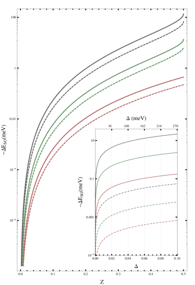
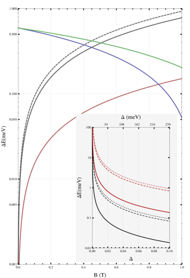
(a) (b)

Figure 1: (Color online) (a) SOI energies as function of $\overline{Z}$ at gap parameter $\overline{{\Delta}}=0.1$ (straight lines) and $\overline{{\Delta}}=0.01$ (dashed lines) for the three lowest-lying energy levels, namely, from top to bottom, $[n,j]\equiv[0,1/2],[1,-1/2]\equiv[1,+1/2]$ and $[0,-3/2]\equiv$ $[0,3/2]$, respectively. Inset shows its dependence on $\overline{{\Delta}}$ at $\overline{Z}$ $=0.1$ (dashed lines) and $\overline{Z}$ $=0.4$ (straight lines), respectively, for the same levels. (b) Relativistic (bold black line) and non-relativistic (dashed black line) Zeeman splitting energies in $[1,-1/2]$ , $[1,+1/2]$ levels, together with their difference (red straight line) as function of magnetic field at fixed value $\overline{Z}=0.3$. For this value of $\overline{Z}$ , we also plot individual SOI for each level, i.e., $[1,-1/2]$ (green), $[1,+1/2]$ (Blue) as function of magnetic field. Inset: relativistic (dashed lines) and nonrelativistic (dotted lines) Zeeman energies together with their difference (bold straight lines) as function of gap parameter for two different magnetic field values, i.e., $B=0.1\,\text{T}$ (black) and $1\,\text{T}$ (Red), respectively.

In the presence of uniform magnetic field, as is seen from Eq. (6), the orbital degeneracies are lifted. In particular, it splits the first excited doubly degenerate $j$ levels, and thus leads to Zeeman splitting. By increasing the magnetic field, as expected, the Zeeman splitting spacing broadens gradually with $B$, (FIG. 1(b)). To show the combined effects of magnetic field on SOI together with the effect of SOI on Zeeman splitting, we plot the Zeeman splitting for the first excited state in the relativistic spectrum as function of magnetic field in FIG. 1(b). We also include a corresponding curve for the non-relativistic energy spectrum as a reference. Hence, by just taking the difference between these two, i.e., between the relativistic and the non-relativistic energies Zeeman energies, we obtain the contribution of SOI energy to the Zeeman splitting energy. Its dependence on $B$, magnetic field dependence of SOI for $j=1/2$ and $j=-1/2$ levels are individually displayed in FIG. 1(b) for comparison. We can see that its influence becomes significant for decreasing $B$, since the Zeeman splitting linearly depend on $B$ and $j$. Therefore, the difference between these two curves is simply the SOI contribution to the Zeeman energy. To learn the response of SOI to the applied magnetic field, we have also plotted the individual SOI energies for each level. Obviously, we claim that, when the associated Zeeman splitting is resolved in an experiment, the related SOI contribution, and therefore SOI energies for each level can be resolved. As an example, at $B=1\mathrm{T}$, our calculation describes Zeeman energy up to $0.70\,\mathrm{meV}$ which contains $0.15\,\mathrm{meV}$ due to SOI. One can also justify this value by just taking the difference between the SOI energies of the related levels which are $0.20\,\mathrm{meV}$ and $0.05\,\mathrm{meV}$ , respectively. As for the inset of the figure, we compare $\overline{{\Delta}}$ dependency of the SOI energies. Eventually, we give a measure of how amount of Zeeman energy is influenced by SOI. The above values may be enhanced by just increasing $\overline{{Z}}$ and/or $\overline{{\Delta}}$ decreasing .

A similar procedure developed above for binding in the hydrogenic sense can also be extended to the binding in oscillatory sense, in the absence of any impurity. In pristine graphene, massless Dirac Fermions having linear dispersion obey Dirac-Weyl equation, and they have no nonrelativistic analog. But, we may overcome this difficulty by just using the spectrum of Dirac equation, and then take its limit when $\overline{{\Delta}}\rightarrow 0$. To do this, it is enough to recall the well-known graphene Landau levels (LLs), i.e.,

$$\overline{E}=\sqrt{\overline{M}_{0}^{2}+2n/\overline{\ell}_{B}^{2}}$$

with $n=\nu+\left(\left|m\right|+m+s+1\right)/2$.  Here. $\overline{\ell}_{B}=1/\sqrt{\overline{B}}$ is the magnetic confinement length. It can easily be shown that its non-relativistic counterpart has energy spectrum with

$$\ \overline{E}_{\mathrm{n.r.}}=\frac{1}{\overline{M}_{0}\overline{\ell}_{B}^{2}}\left(\nu+\frac{\left|m\right|+m+1}{2}\right)+\frac{g\ast s}{\overline{M}_{0}\overline{\ell}_{B}^{2}}$$

(a)

Figure 2: (Color online) For the four lowest eigenstates of the graphene, SOI energies as function of gap parameter  at $B=1\ \mathrm{T}$. The upper scale shows the gap parameter in units of $\mathrm{meV}$. Inset:  SOI for free particle spectrum, i.e., $\Delta\overline{E}_{\mathrm{SO}}=-\overline{M}_{0}+\sqrt{\overline{M}_{0}^{2}+\overline{k}_{0}^{2}}-\left(\overline{k}_{0}^{2}/2\overline{M}_{0}\right)$ as function of gap parameter. From top to bottom, red, green and black straight lines corresponds $\overline{k}_{0}=0.1$, $0.01$, and $0.001$, respectively.

wherein the first term is the well-known non-relativistic LLs, the second one is due to Zeeman effect. Here, we will set the Landé factor to $2$. It is easy to check analytically that SOI energy is zero for $n=0$ ($\nu=0$,$m=0$, $s=-1$) level even without taking $\overline{{\Delta}}\rightarrow 0$ limit (massless limit). It is also easy to see that higher orbital are sensitive to decrease in $\overline{{\Delta}}$, i.e., $\overline{{\Delta}}\rightarrow 0$ limit (gapless limit). As is done in FIG. 2, it is also instructive to compare this picture with those obtained from the free particle spectrum, i.e., $\Delta\overline{E}_{\mathrm{SO}}=-\overline{M}_{0}+\sqrt{\overline{M}_{0}^{2}+\overline{k}_{0}^{2}}-\left(\overline{k}_{0}^{2}/2\overline{M}_{0}\right)$ which is also zero at $\overline{k}_{0}\rightarrow 0$ limit. Again, even in the presence of mass term, it gives zero. Whereas it becomes more pronounced as $\overline{{\Delta}}\rightarrow 0$ for finite $\overline{k}_{0}$. The appearance of the lack of SOI in the electron-hole degeneracy point, i.e., in both $n=0$ and $\overline{k}_{0}=0$ cases, shows that this point has purely non-relativistic character. Furthermore, this proves that the ground-state of the flat graphene does not exhibit SQHE regime. Additionally, beyond this point we see that SOI effects are much more pronounced in $\overline{{\Delta}}\rightarrow 0$ limit than those found for the impurity coverage in the same limit. These findings are exactly compatible with the analytical predictions of the relativistic quantum mechanics on the general form for SOI energy in general. All these show that our predictions work well for different physical regimes.

We have three main conclusions. First, we demonstrate theoretically that, without sophisticated many-body calculations, intrinsic SOI energy in the electron-hole degeneracy point is zero in flat graphene. Thus, we conclude that, for flat graphene, it is not possible to observe SQHE. Second, within the impurity coverage, we investigate the influence of SOI on graphene energy levels. Finally, in the same context, we investigate the Zeeman splitting in doped graphene as well as the influence of SOI on this splitting . We demonstrate that it is possible to enhance intrinsic SOI by increasing the strength of applied magnetic field, and how it can be resolved from the Zeeman effect. Therefore, magnetic field not only can be used to tune the Zeeman effect, but also allow us to estimate the magnitude of the SOI energy in dopped graphene. As for the Zitterbewegung, its effect should be taken account for higher levels and higher magnetic field values. Its signature is the oscillatory behavior of the velocity and for its direct observation stronger magnetic fields would be required Romera2009 . It can also be resolved in the same procedure described here within this context, i.e., but for higher levels where SOI is negligible, and for higher magnetic fields. We hope that this study will not just reveal the intrinsic SOI in graphene, but also it will illuminate the Berry phase in graphene, since very recently it is shown that, by constructing the intrinsic SOI operator from the non-Abelian Berry connection, intrinsic SOI originates from Berry phase terms Bliokh2011 .

- (1) K. S. Novoselov, A. K. Geim, S. V. Morozov, D. Jiang, Y. Zhang, S. V. Dubonos, I. V. Grigorieva, and A. A. Firsov, Science 306, 666 (2004).
- (2) H. Chen, V. Apalkov and T. Chakraborty, Phys. Rev. Lett. 98, 186803 (2005).
- (3) A. Rycerz, J. Tworzylo and C. W. J. Beenakker, Nature Physics. 3, 172 (2007).
- (4) J. H. Badarson, M. Titov,and P.W.Brouwer, Phys. Rev. Lett. 102, 226803 (2009).
- (5) D. Loss and D. P. Di Vincenzo, Phys. Rev. A 57, 120 (1998).
- (6) P. Recher and B. Trauzettel, Nanotechnology, 21, 302001 (2010).
- (7) C. L. Kane and E. J. Mele, Phys. Rev. Lett. 95, 226801 (2005).
- (8) Daniel Huertas-Harnendo, F. Guinea, and A. Brataas, Phys. Rev. B 74, 155426 (2006).
- (9) Hongki Min, J. E. Hill, N. A. Sinitsyn, B. R. Sahu, Leonard Kleinman and A. H. MacDonald, Phys. Rev. B 74, 165310 (2006).
- (10) F. Kuemmeth, S. Ilani, D.C. Ralph and P. L. McEuen, Nature 452, 448 (2008).
- (11) Emmanuel I. Rashba, Phys. Rev.B 79, 161409(R) (2009).
- (12) Daniel Huertas-Harnendo, F. Guinea, and A. Brataas, Phys. Rev. Lett. 103, 146801 (2009).
- (13) A. H. Castro Neto and F. Guinea, Phys. Rev. Lett. 103, 026804 (2009).
- (14) M. Gmitra, S. Konschuh, C. Ertler, C. Ambrosch-Draxl and J. Fabian, Phys. Rev. B 80, 235431 (2009).
- (15) P. Rakyta, A. Kormányos, and J. Cserti, Phys. Rev. B 82, 113405 (2010).
- (16) M. P. López-Sancho, and M. C. Muñoz, Phys. Rev. B 83, 075406 (2011).
- (17) D. A. Abanin, R. V. Gorbachev, K. S. Novoselov, A. K. Geim, and L. S. Levitov, Phys.Rev. Lett. 107, 096601 (2011).
- (18) Konstantin Y. Bliokh, Mark R. Dennis, and Franco Nori, Phys. Rev. Lett. 107, 174802 (2011).
- (19) Ming-Hao Liu, Jan Bundesmann, and Klaus Richter, Phys. Rev. B 85, 085406 (2012).
- (20) Matthew Mecklenburg and B. C. Regan, Phys.Rev. Lett. 106, 116803 (2011).
- (21) Quantum Mechanics, Volume II, Albert Messiah, translated from the French by J. Potter, North-Holland Publishing Company, Amsterdam, 1961 (Holland) pp 944.
- (22) Quantum Electrodynamics, edited by V.B. Berestetskii, E.M. Lifshitz, and L.P. Pitaevskii, Pergamon Press, second ed., 1982 (Great Britain) pp 123.
- (23) Relativistic Quantum Mechanics, James D. Björken and Sidney D. Drell, McGraw-Hill Inc., 1964 (United States of America) pp 52.
- (24) D. S. Novikov, Phys. Rev. B 76, 245435 (2007).
- (25) Ming-Hao Liu, Jan Bundesmann, and Klaus Richter, Phys.Rev. A 61, 032104 (2000).
- (26) Relativistic Quantum Mechanics, Paul Strange, Cambridge University Press, 1998 (UK) pp 240.
- (27) E. Romera, and F. de los Santos, Phys.Rev. B 80, 165416 (2009).
- (28) Konstantin Y. Bliokh, Mark R. Dennis, and Franco Nori, Phys. Rev. Lett. 107, 174802 (2011).