Chiral Polaron Formation in Graphene

Abstract

A theoretical investigation of the possible existence of the chiral polaron formation in graphene is reported. We present an analytical method to calculate the ground-state of the electron-phonon system within the framework of the Lee-Low and Pines theory. On the basis of our model, the influence of electron-optical phonon interaction onto the graphene electronic spectrum is examined. In this paper, we only considered doubly degenerate optical phonon modes of $\mathrm{E}_{2g}$ symmetry near the zone center $\Gamma$. We show analytically that the energy dispersions of both valance and conduction bands of the pristine graphene differ significantly than those obtained through the standard electron self energy calculations due to the electron-phonon interactions. Furthermore, we prove that the degenerate band structure of the graphene promote the chiral polaron formation.

Since the discovery of graphene Novoselov2004 , many studies have focused on electron-phonon interactions, because of their particular importance in understanding electronic and optical properties of graphene Lazzeri2005 ; Lazzeri2006 ; Pisana2007 ; Yan2007 ; Calandra2007 ; Basko2008 ; Stauber2008a ; Vladimir2010 ; Goerbig2007 ; Basko2007 ; Basko2008r ; Lazzeri2008 ; Mariani2008 ; Faugeras2009 ; Carbotte2010 ; Mariani2010 ; Hwang2010 ; Ping2012 ; Araujo2012 . Even though the interaction of electron with doubly degenerate optical phonon modes of $\mathrm{E}_{2g}$ symmetry near the zone center $\Gamma$ does not open a gap Pisana2007 ; Dubay2003 , they contribute significantly to intravalley-intraband and intravalley-interband scattering Rana2009 . Since these phonon modes consist of in-plane out-of-phase displacements of two sublattices A and B, they just shift the $\mathrm{K}$ ($\mathrm{K}^{{}^{\prime}}$) point so as to electronic bands are still described by Dirac cones Pisana2007 . Moreover, it is also revealed that the gate-modulated low-temperature Raman spectroscopy, the graphene G band, which is the optical phonon at long wavelength, is markedly sensitive to the coupling with Dirac fermion excitations at small wave vectors (long wavelengths) Yan2007 .

So far only perturbational methods for intraband transitions have been applied to the electron-phonon interactions, the combined effect of intra- and inter-band scattering in a single valley has not been considered. Due to the fact that graphene is a semimetal, actually gapless or zero-gap semiconductor, the Dirac cones can not be treated independently for electron-$\mathrm{E}_{2g}$ phonon interactions. Single band approximations take into account the intraband transitions only and they ignore the lack of gap, thus omit the electron (hole) transitions from $\pi$ $(\pi^{\ast})$ valance (conduction) to $\pi^{\ast}$($\pi$ ) conduction (valance) bands. Whereas, due to the lack of gap, $\mathrm{E}_{2g}$ phonon can easily excite electron-hole pairs leading to the chirality dependent modifications in carrier dynamics.

In this letter, we used the continuum Fröhlich type model to treat the interaction of electron with long wavelength $\mathrm{E}_{2g}$ phonon. We introduce a diagonalization procedure based on Lee-Low-Pines (LLP) like transformations to investigate the properties of both valance and conduction band polarons in graphene. Within the framework of low-energy continuum model of graphene, the Hamiltonian of an electron interacting with optical $\Gamma$-phonon around the $\mathbf{K}$ point in the Brillouin zone can be written as

$$\mathcal{H}=\mathcal{H}_{0}+\sum_{\bm{q}}\hbar\omega_{\mu}(\bm{q})b_{\bm{q\mu}}^{{\dagger}}b_{\bm{q\mu}}+\mathcal{H}_{e-p},$$ (1)

where $\mathcal{H}_{0}=v_{F}\bm{\sigma}\cdot\bm{p}$ is the unperturbed bare Hamiltonian, whose spectrum describes cone like behavior with eigenvalues $\epsilon_{k\lambda}=\lambda\epsilon_{k}$ wherein $\epsilon_{k}=v_{F}k$ and $\lambda$ is the chirality index, together with the corresponding eigenkets $\left|\bm{k}\lambda\right\rangle=\exp(i\bm{k}\cdot\bm{r})\left(\begin{array}[]{cc}0&\lambda e^{i\theta\left(\bm{k}\right)}\end{array}\right)^{{\dagger}}/\sqrt{2}L.$

In Eq.(1), $\mathcal{H}_{e-p}$ is the electron-optical phonon interaction Hamiltonian Basko2008 ; Lazzeri2008 ; Ando2006b , and is given by

$$\mathcal{H}_{e-p}=-\sum_{\bm{q}}\left[\widetilde{\mathrm{M}}_{\mu}^{\mathbf{K}}\left(\bm{q}\right)b_{\bm{q\mu}}e^{i\bm{q\cdot r}}+\mathrm{H.c.}\right],$$ (2)

where $b_{\bm{q\mu}}^{{\dagger}}\left(b_{\bm{q\mu}}\right)$ is the optical phonon creation (annihilation) operator with longitudinal and transverse optical phonon branch index $\mu=1$ (LO) and $2$ (TO), respectively. Their dispersion have the form $\omega_{\mu}\left(\bm{q}\right)=\omega_{\Gamma}\left(0\right)R_{\mu}\left(qa\right)$ with dimensionless part $R_{\mu}\left(qa\right)=\ \left[1-r_{\mu}\left(qa\right)\right]^{1/2}$, and with $\omega_{\Gamma}\left(0\right)=0.196$ $eV$, where $r_{1}$ and $r_{2}$ are given by $0.1138$ and $0.01979$, respectivelyStauber2008b . The momentum dependent matrix element of the interaction Eq.(2) is $\widetilde{\mathrm{M}}_{\mu}^{\mathbf{K}}\left(\bm{q}\right)=\overline{\mathrm{M}}_{\mu}^{\mathbf{K}}\left(\bm{q}\right)\mathrm{M}_{\mu}\left(\bm{q}\right)$ , and defined as

$$\mathrm{M}_{\mu}\left(\bm{q}\right)=\left[\begin{array}[]{cc}0&\mathrm{M}_{\mathrm{BA}}e^{-i\phi\left(\bm{q}\right)}\\ \mathrm{M}_{\mathrm{AB}}e^{i\phi\left(\bm{q}\right)}&0\end{array}\right]$$ (3)

with $\mathrm{M}_{\mathrm{AB}}=+1(i)$ and $\mathrm{M}_{\mathrm{BA}}=-1(i)$  for LO(TO) phononsTse2007 . $\phi\left(\bm{q}\right)=\tan^{-1}\left(q_{y}/q_{x}\right)$ is the azimuthal angle of the phonon wave vector $\bm{q,}$ and $\overline{\mathrm{M}}_{\mu}^{\mathbf{K}}\left(\bm{q}\right)=\overline{\mathrm{M}}/\sqrt{NR_{\mu}\left(qa\right)}$ with $\overline{\mathrm{M}}=3a_{0}q_{0}J_{0}/\sqrt{2}$. Here, $q_{0}=\left(\partial J_{0}/\partial a\right)/J_{0}$ is predictedPietronero1980 ; Jishi1993 around $2$ $\mathring{A}^{-1}$ or $2.5$ $\mathring{A}^{-1}$.

To solve Eq.(1), we propose a diagonalization procedure based on the LLP method, which includes two successive unitary transformations. Pristine graphene has a electron-hole degeneracy point at $k=0$. Therefore, to be compatible with this gapless band structure of the graphene, we make an ansatz for the chiral polaron ground-state vector

$$\left|\bm{\Phi}\right\rangle_{pol}=U_{1}U_{2}\left|\bm{0}\right\rangle_{ph}\otimes\left|\bm{\pm}\right\rangle$$ (4)

such that $\mathcal{H}\left|\bm{\Phi}\right\rangle_{pol}=E_{\pm}\left|\bm{\Phi}\right\rangle_{pol}$. In Eq.(4), $\left|\bm{0}\right\rangle_{ph}$ stands for the phonon vacuum, and $\left|\bm{\pm}\right\rangle$=$\sum_{\lambda}\alpha_{\pm}^{\lambda}\left|\bm{k}\lambda\right\rangle$ corresponds to electronic state vector defined through the appropriate fractional amplitudes, $\alpha_{\pm}^{\lambda}$, due to the fact that polaronic wavefunction must be the linear combination of $\left|\bm{k}+\right\rangle$ and $\left|\bm{k}-\right\rangle$, respectively. While the first unitary transformation

$$U_{1}=\exp\left[-i\bm{r\cdot}\sum_{\bm{q}}\bm{q}b_{\bm{q\mu}}^{{\dagger}}b_{\bm{q\mu}}\right]$$

eliminates the electron coordinates, since the transformed operators are given by the relations, $\widetilde{b}_{\bm{q\mu}}=b_{\bm{q\mu}}\exp\left[-i\bm{q\cdot r}\right]$ and $\widetilde{\bm{p}}\bm{=p}-\sum_{\bm{q}}\hbar\bm{q}b_{\bm{q\mu}}^{{\dagger}}b_{\bm{q\mu}}$, second unitary transformation

$$U_{2}=\exp\left\{\sum_{\bm{q}}\left[\overline{\mathrm{M}}_{0\mu}^{\ast}\left(\bm{q}\right)\left\langle\bm{k}\lambda^{{}^{\prime}}\right|\mathrm{M}_{\mu}^{{\dagger}}\left(\bm{q}\right)\left|\bm{k}\lambda\right\rangle b_{\bm{q\mu}}^{{\dagger}}-\mathrm{H.c.}\right]\right\}$$

is the displaced oscillator transformation with amplitude $\overline{\mathrm{M}}_{0\mu}\left(\bm{q}\right)=\overline{\mathrm{M}}_{\mu}^{\mathbf{K}}\left(\bm{q}\right)$/$\hbar\omega_{\mu}(\bm{q})$. It just shifts the phonon coordinates. As a result, the transformed Hamiltonian can be written as $\widetilde{\mathcal{H}}=$ $U_{2}^{-1}U_{1}^{-1}\mathcal{H}U_{1}U_{2}.$ Therefore, ${}_{ph}\left\langle\bm{0}\right|\widetilde{\mathcal{H}}\left|\bm{0}\right\rangle_{ph}$ leads to the following equation:

$${}_{ph}\left\langle\bm{0}\right|\widetilde{\mathcal{H}}\left|\bm{0}\right\rangle_{ph} = v_{F}\bm{\sigma}\cdot\left(\bm{p-}\hbar\sum_{\bm{q}}\bm{q}\left|\overline{\mathrm{M}}_{0\mu}\left(\bm{q}\right)\right|^{2}\left|\left\langle\bm{k}\lambda^{{}^{\prime}}\right|\mathrm{M}_{\mu}^{{\dagger}}\left(\bm{q}\right)\left|\bm{k}\lambda\right\rangle\right|^{2}\right)$$

$$+\sum\limits_{\bm{q}}\hbar\omega_{\mu}(\bm{q})\left|\overline{\mathrm{M}}_{0\mu}\left(\bm{q}\right)\right|^{2}\left|\left\langle\bm{k}\lambda^{{}^{\prime}}\right|\mathrm{M}_{\mu}^{{\dagger}}\left(\bm{q}\right)\left|\bm{k}\lambda\right\rangle\right|^{2}-\sum\limits_{\bm{q}}\left[\mathrm{M}_{\mu}\left(\bm{q}\right)\left|\overline{\mathrm{M}}_{0\mu}\left(\bm{q}\right)\right|^{2}\left|\left\langle\bm{k}\lambda^{{}^{\prime}}\right|\mathrm{M}_{\mu}^{{\dagger}}\left(\bm{q}\right)\left|\bm{k}\lambda\right\rangle\right|^{2}+\mathrm{H.c.}\right].$$

Finally, by using the ansatz given by Eq.(4), one can easily construct characteristic equation of the matrix in the form

$$\left|\begin{array}[]{cc}E_{\pm}-\hbar v_{F}k\bm{+}\hbar v_{F}\bm{\Sigma}_{++}(\mu,k)+\bm{\Sigma}_{++}^{0}(\mu,k)&\hbar v_{F}\bm{\Sigma}_{+-}(\mu,k)+2\bm{\Sigma}_{+-}^{0}(\mu,k)\\ \hbar v_{F}\bm{\Sigma}_{-+}(\mu,k)+2\bm{\Sigma}_{-+}^{0}(\mu,k)&E_{\pm}+\hbar v_{F}k\bm{+}\hbar v_{F}\bm{\Sigma}_{--}(\mu,k)+\bm{\Sigma}_{--}^{0}(\mu,k)\end{array}\right|=0$$ (7)

with elements

$$\left.\begin{array}[]{c}\bm{\Sigma}_{++}(\mu,k)\\ \bm{\Sigma}_{+-}(\mu,k)\end{array}\right\} = \frac{1}{2}\sum\limits_{\bm{q}}\left|\overline{\mathrm{M}}_{0\mu}\left(\bm{q}\right)\right|^{2}$$ (10)

$$\times \left[1\pm s_{\mu}\cos 2\left(\theta-\phi\right)\right]\left\{\begin{array}[]{c}\bm{q}_{\mu}\cos\left(\theta-\phi\right)\\ \bm{iq}\sin\left(\theta-\phi\right)\end{array}\right.,$$ (13)

$$\bm{\Sigma}_{\lambda\lambda^{{}^{\prime}}}^{0}(\mu,k) = \frac{1}{2}\sum\limits_{\bm{q}}\left|\overline{\mathrm{M}}_{0\mu}\left(\bm{q}\right)\right|^{2}$$ (14)

$$\times \hbar\omega_{\mu}(\bm{q})\left[1+s_{\mu}\lambda\lambda^{{}^{\prime}}\cos 2\left(\theta-\phi\right)\right],$$

where $\bm{\Sigma}_{--}=-\bm{\Sigma}_{++}$ and $\bm{\Sigma}_{-+}=\bm{\Sigma}_{+-}^{\ast}$.  After converting the sums in Eq.(14) into integrals over $\bm{q,}$ it is easy to see that the terms with $\bm{\Sigma}_{\lambda\lambda^{{}^{\prime}}}(\mu,k)$ do not give contribution to the eigenvalue calculation, since they all vanish after the $\bm{q}$ integration. But the rest, i.e., terms with $\bm{\Sigma}_{\lambda\lambda^{{}^{\prime}}}^{0}(\mu,k)$ contribute. Thus, from the secular equation, i.e., from Eq.(7) the eigenvalues $E_{\pm}$ can then be solved analytically as a function of $k$ in closed form,      

$$E_{\pm}=\pm\left\{\left(\hbar v_{F}k\right)^{2}+4\left[\bm{\Sigma}_{\pm\mp}^{0}(\mu,k)\right]^{2}\right\}^{1/2}-\bm{\Sigma}_{\pm\pm}^{0}(\mu,k).$$ (15)

In Eq.(15), while the last term is due to the intraband transitions, second one in the parenthesis is contribution due to the coupling between valance and conduction bands, i.e. it corresponds to interband transitions. Thus, our chiral polaron dispersion consists of partial mixture of contributions from valance and conduction bands. While taking the integrals in Eq.(15), since they diverge at upper limit of the integrations, we must introduce an upper cut-off frequency in the integrations to make them to be finite. It is nothing but just $2k$, due to $q\in\left[0,2k\right]$. As a result,one obtains $k-$dependent contributions as

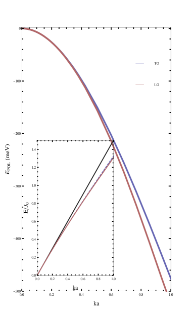
Figure 1: (Color online) The polaron ground-state energy obtained from Eq.(15) as a function of $\overline{k}_{0}\bm{=}ka$. Inset: shows the electron dispersion normalized to $J_{0}$ as a function of $\overline{k}_{0}\bm{=}ka$.

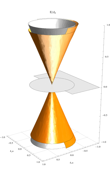
Figure 2: Electron-hole band dispersions as a function of $\overline{k}_{0}\bm{=}ka$ both in the absence of (inner cone) and in the presence of electron (hole)- phonon interaction (outer cone). Only LO phonon contribution is taken into account. The thick dark circle on the $E/J_{0}=0$ plane is the projection of both perturbed (lower contour in the upper cone) and unperturbed (upper contour in the upper cone) the contour at $E/J_{0}=1$. It is drawn to guide to eye how the dressed polaronic band dispersions differ from the undressed ones.

$$\bm{\Sigma}_{\lambda\lambda^{{}^{\prime}}}^{0}(\mu,k)=\frac{3\sqrt{3}}{4\pi r_{\mu}}J_{0}\alpha\left(0\right)\ln\left[\frac{1}{1-r_{\mu}\left(2\overline{k}_{0}\right)^{2}}\right],$$ (16)

where we have defined $\alpha\left(0\right)=\left|\overline{\mathrm{M}}\right|^{2}/4J_{0}\hbar\omega_{\Gamma}(0)$ and new dimensionless wave vector, $\overline{k}_{o}=ka$. $\alpha\left(0\right)$ is of order of $0.054\left(0.089\right)$ depending on the choice of $q_{0}=2\left(2.5\right)$ $\mathring{A}^{-1}$.We analyze Eq.(15) in FIG. 1, which shows both polaron self energy and Fermi velocity renormalization. As it can be easily seen from the figure that polaron self energy is strongly enhanced with increase in $\overline{k}_{o}$. This can also be justified from its inset that shows how electron-phonon interactions renormalize the Dirac velocity. To see this clearly we also present in FIG. 2 electron-hole band dispersions as a function of $\overline{k}_{0}\bm{=}ka$ both in the absence and presence of electron (hole)- phonon interactions.

It is convenient to rewrite Eq.(16) for small $k$’s, which corresponds to neglect phonon dispersions, i.e., it results with polaron dispersion independent on $r_{\mu}$. To do this, we first expand the logarithm in Eq.(16), in power series of $k$ , and then replace the resultant back into Eq.(16)so that Eq.(15) reduces to the simple form

$$\overline{E}_{\pm}=\pm\overline{k}_{o}\left\{1+4\left[\frac{2\sqrt{3}}{\pi}\alpha\left(0\right)\overline{k}_{0}\right]^{2}\right\}^{1/2}-\frac{2\sqrt{3}}{\pi}\alpha\left(0\right)\overline{k}_{0}^{2},$$ (17)

where $\overline{E}_{\pm}=aE_{\pm}/\hbar v_{F}$ is the dimensionless energy. The standard electron-self energy calculations due to the interactions of electron with degenerate optical phonon modes with E_2g symmetry in graphene predict a lowering of both conduction and valance band energies in the same direction to preserve the symmetry of the Dirac cones. Whereas, in our case, as $\overline{k}_{o}$ increases, negativity due to intraband interactions is compensated by  the second term in the parenthesis in Eq.(16), i.e., by the interband interactions. Although it is compensated, their combined effects strongly modify the Dirac cones (FIG. 2 ). Since Eq.(15) can easily be rearranged into the form $\overline{E}_{\lambda}=\lambda\hbar\widetilde{v}_{F}\left(\overline{k}_{0}\right)\overline{k}_{0}$ , we can thus define the renormalized Fermi velocity as

$$\widetilde{v}_{F}\left(\overline{k}_{0}\right)=v_{F}\left[\sqrt{1+4\widetilde{\alpha}^{2}\left(\overline{k}_{0}\right)}\mp\widetilde{\alpha}\left(\overline{k}_{0}\right)\right],$$

wherein, in analogy with quantum chromodynamicsGRIFFITHS1987 , we also define a new coupling constant, running coupling constant, as a function of $k$, i.e, energy,

$$\widetilde{\alpha}\left(\overline{k}_{0}\right)=\frac{2\sqrt{3}}{\pi}\alpha\left(0\right)\overline{k}_{0}.$$

In conclusion, we predict a new type of polaronic formation in pristine graphene. We demonstrate that our results are differ from those obtained through standard electron self energy calculations due to electron-E_2g phonon interactions in nondegenerate band case. We show that chiral polaron band dispersions consist of k dependent terms besides the free undressed one. In addition to free undressed ones, both intraband and interband interactions coexist in a one polaron dispersion. Moreover, a considerable renormalization of Fermi velocity, i.e., slope of Dirac cones in graphene is observed due to the electron-optical phonon interactions in graphene. It is also found that, the effect of LO phonon-electron interaction is stronger than that of TO. As for the validity of our approximation it is valid for $\overline{k}_{0}\bm{=}ka<1,$ however it can be extended to higher $k$ values by just including the effect of trigonal warping in the total Hamiltonian. It can also be extended to the case electron-$\mathbf{K}$ phonons interaction where a gap occurs. Furthermore, it can also be generalized to the calculation of phonon induced electron-hole or electron-electron interactions, i.e., to exciton or bipolaron binding energies in graphene.

References

• (1) K. S. Novoselov, A. K. Geim, S. V. Morozov, D. Jiang, Y. Zhang, S. V. Dubonos, I. V. Grigorieva and A. A. Firsov, Science 306, 666 (2004);K. S. Novoselov , D. Jiang , F. Schedin , T. J. Booth , V. V. Khotkevich , S. V. Morozov , and A. K. Geim ,Proc. Nat. Acad. Sci. USA 102,10451 (2005).
• (2) Michele Lazzeri, S. Piscanec, Francesco Mauri, A. C. Ferrari, and J. Robertson, Phys. Rev. Lett. 95 236802, (2005).
• (3) Michele Lazzeri, S. Piscanec, Francesco Mauri, A. C. Ferrari2, and J. Robertson, Phys. Rev. B 73, 155426 (2006).
• (4) Simone Pisana, Michele Lazzeri, Cinzia Casiraghi, Kostya S. Novoselov, A. K. Geim, Andrea C. Ferrari and Francesco Mauri, Nature Materials, 6,198 (2007).
• (5) Jun Yan, Yuanbo Zhang, Philip Kim, and Aron Pinczuk ,Phys. Rev. Lett. 98, 166802 (2007)
• (6) Matteo Calandra and Francesco Mauri, Phys Rev. B 76,205411 (2007).
• (7) D. M. Basko, Phys. Rev. B 78125418 (2008).
• (8) T Stauber and N M R Peres, J. Phys.:Condensed Matter 20,055002, (2008)
• (9) Vladimir M. StojanoviΔ‡ and Nenad VukmiroviΔ‡, Phys. Rev. B 82, 165410, (2010).
• (10) M. O. Goerbig, J.-N. Fuchs, K. Kechedzhi and Vladimir I. Fal’ko, Phys. Rev. Lett. 99, 087402 (2007).
• (11) D. M. Basko, Phys. Rev. B 76, 081405 (R) (2007).
• (12) D.M. Basko, I.L. Aleiner, Phys. Rev. B 77 (2008) 041409(R).
• (13) Michele Lazzeri, Claudio Attaccalite, Ludger Wirtz, and Francesco Mauri, Phys. Rev. B 78, 081406 (R), (2008).
• (14) Eros Mariani and Felix von Oppen, Phys. Rev. Lett. 100, 076801 (2008).
• (15) C. Faugeras, M. Amado, P. Kossacki, M. Orlita, M. Sprinkle, C. Berger, W. A. de Heer, and M. Potemski, Phys. Rev. Lett. 103, 186803, (2009).
• (16) Carbotte, J. P., Nicol, E. J., and Sharapov, S. G., Phys. Rev. B 81,045419, (2010).
• (17) Eros Mariani and Felix von Oppen, Phys. Rev. B. 82, 195403, (2010).
• (18) E. H. Hwang, Rajdeep Sensarma, and S. Das Sarma, Phys. Rev. B 82, 195406, (2010).
• (19) Wei-Ping Li, Zi-Wu Wang, Ji-Wen Yin and Yi-Fu Yu, J. Phys.: Condensed Matt. 24, 135301, (2012).
• (20) P. T. Araujo, D. L. Mafra, K. Sato, R. Saito, J. Kong and M. S. Dresselhaus, arxiv:1203.0547v1 (2012).
• (21) O. Dubay and G. Kresse, Phys. Rev. B 67, 035401 (2003)
• (22) Farhan Rana, Paul A. George, Jared H. Strait, Jahan Dawlaty, Shriram Shivaraman, Mvs Chandrashekhar, and Michael G. Spencer, Phys. Rev. B 79, 115447 (2009).
• (23) Tsuneya Ando,J. Phys. Soc. Jpn. 75, 084713 (2006).
• (24) Kohta Ishikawa and Tsuneya Ando, J. Phys. Soc. Jpn. 75, 14701 (2006).
• (25) T. Stauber, N. M. R. Peres, and A. H. Castro Neto, Phys. Rev. B 78, 085418 (2008).
• (26) Wang-Kong Tse and S. Das Sarma, Phys. Rev. Lett. 99, 236802 (2007).
• (27) L. Pietronero, S. StrΓ€ssler, and H. R. Zeller, M. J. Rice, Phys. Rev. B 22, 904–910 (1980)
• (28) R. A. Jishi, M. S. Dresselhaus and G. Dresselhaus, Phys. Rev. B 48, 11385–11389 (1993).
• (29) Introduction to elementary particles, David Griffiths, John Wiley and Sons, Inc., 1987 (Singapore) pp 249.