Many-particle Systems in One Dimension in the Harmonic Approximation

Abstract

We consider energetics and structural properties of a many particle system in one dimension with pairwise contact interactions confined in a parabolic external potential. To render the problem analytically solvable, we use the harmonic approximation scheme at the level of the Hamiltonian. We investigate the scaling with particle number of the ground state energies for systems consisting of identical bosons or fermions. We then proceed to focus on bosonic systems and make a detailed comparison to known exact results in the absence of the parabolic external trap for three-body systems. We also consider the thermodynamics of the harmonic model which turns out to be similar for bosons and fermions due to the lack of degeneracy in one dimension.

I Introduction

Exactly solvable models are key players in few- and many-body quantum mechanics and are indeed also fascinating creatures mattis ; sutherland . The analytical intractability of general $N$-body systems makes it extremely important to have exact results to allow benchmark tests of complicated numerical methods. Unfortunately, exactly solvable models are few and far between and are more often found in low-dimensional systems. In the case of one spatial dimension, the famous Bethe ansatz bethe1931 was succesfully applied to models of bosons with zero-range interactions lieb1963a ; lieb1963b ; macguire1964 , and later to interactions with long range sutherland1971 ; calogero1971 .

Meanwhile, an exciting direction in the field of cold atomic gases aims at the study of low-dimensional systems in general and one-dimensional setups in particular bloch2008 . A noticable highlight of this pursuit is the experimental realization of the so-called Tonks-Girardeau gas paredes2004 ; kinoshita2004 ; haller2009 , where strongly-interacting one-dimensional bosons become impenetrable objects and behave similar to fermions tonks1936 ; girardeau1960 . Very recently, it has even become possible to study this interesting regime in the limit of small particle number serwane2011 ; zurn2012 .

Here we study an exactly solvable model of an $N$-body system in an external parabolic confinement. The outer trap is always present in cold atomic gas experiments but can often be neglected or treated in a local density approximation when large systems are studied. However, for smaller particle numbers the effect of the outer trap becomes important for the structure and dynamics of the system. To make the $N$-body problem tractable we use a harmonic Hamiltonian approximation calogero1971 with carefully chosen parameters that reproduce essential features of two atoms interacting via short-range interactions in a parabolic trap arms11 .

The paper is organized as follows. After a discussion of the harmonic methods we provide details on how the parameters of the harmonic interactions are obtained from knowledge of the exact solution of the two-body problem originally obtained by Busch et al. busc98 . We then present results for the ground-state energies and the radii. Our focus is on bosonic systems, but we do present a few results for fermions as well. A comparison to the exact results of MacGuire macguire1964 is then made in relevant limits. We also compute the one-body density matrix and its largest eigenvalue to obtain the condensate fraction at zero temperature. Lastly, we discuss the thermodynamics of our model and then proceed to conclusion and outlook for future work.

II Method

We consider a system of $N$ quantum particles interacting pairwise via a delta function interaction and confined by a harmonic external potential in one-spatial dimension. The Hamiltonian for this system is

$$H=-\frac{\hbar^{2}}{2m}\sum_{i=1}^{N}\frac{\partial^{2}}{\partial x_{i}^{2}}+\frac{1}{2}m\omega_{0}^{2}\sum_{i=1}^{N}x_{i}^{2}-\frac{2\hbar^{2}}{ma}\sum_{i<k}\delta^{1D}(x_{i}-x_{k}),$$ (1)

where $m$ is the mass of the particles, $\omega_{0}$ is the frequency of the external field, and $a$ is the one-dimensional scattering length which parameterizes the strength of the two-body interaction (we will discuss its relation to the three-dimensional scattering length below). The external field, $\omega_{0}$, defines the length scale of our system, $l^{2}=\hbar/(m\omega_{0})$. For two particles, (1) has been solved in, e.g., busc98 ; farr10 , and their results of two-body energies and wave functions for a given scattering length are used to determine the parameters of our model. We consider only the bound molecular branch of the system, i.e., $a>0$.

In our general harmonic approximation scheme we replace Hamiltonian (1) with

$$H = -\frac{\hbar^{2}}{2m}\sum_{i}^{N}\frac{\partial^{2}}{\partial x_{i}^{2}}+\frac{1}{2}m\omega_{0}^{2}\sum_{i}^{N}x_{i}^{2}$$ (2)

$$+\frac{1}{2}\mu\omega_{in}^{2}\sum_{i<k}(x_{i}-x_{k})^{2}+\sum_{i<k}V_{S},$$

where $\mu=m/2$ is the reduced mass of the two-body system, $\omega_{in}$ is the interacting frequency, and $V_{S}$ is an energy shift. The solution to this equation for $N$ particles for general systems is described in detail in arms11 and more specifically for identical particles in calogero1971 and arms12 .

The parameters $\omega_{in}$ and $V_{S}$ are now chosen to fit pertinent properties of the original Hamiltonian at the two-body level in the usual spirit of constructive descriptions of $N$-body systems based on two-body interactions. Here we impose the condition that at the two-body level the harmonic oscillator reproduces the energy and average square radius of the exact two-body solution. In order to fulfil these constraints, we use the size of the system to determine the interaction frequency through the relation

$$\frac{\langle\psi|x^{2}|\psi\rangle}{\langle\psi|\psi\rangle}=\frac{\hbar}{2\mu\sqrt{\omega_{in}^{2}+\omega_{0}^{2}}},$$ (3)

where $x=x_{1}-x_{2}$ is the relative coordinate in the two-body system. The energy shift is determined by requiring that the model reproduces the energy of the two-body system

$$E_{2}=\frac{1}{2}\hbar\sqrt{\omega_{in}^{2}+\omega_{0}^{2}}+V_{S}.$$ (4)

The quantities $E_{2}$ and $\langle x^{2}\rangle$ can be easily obtained by numerically solving the transcendental equations fulfilled by the exact solution for two bosons (or two fermions in different spin states) interacting via a zero-range interaction in a parabolic trap busc98 . Note that when we consider identical fermions below, there can in principle only be a non-zero two-body interaction in states that are odd under exchange of the two fermions. In this paper we are mostly interested in the scaling behaviour with particle number of the fermions as the interaction frequency is varied (through the scattering length) and we therefore ignore this point and use the same input for fermions as for bosons. The most important difference is of course the quantum statistics which is taken fully into account.

We note that in cold atoms, effective one-dimensional setups are created by using a tightly confining potential in two transverse directions, usually through the application of an optical lattice bloch2008 . In a deep transverse lattice, the atoms are then effectively only occupying the lowest transverse motional degree of freedom. This transverse degree of freedom, however, has an influence on the effective one-dimensional scattering length that described the inter-atomic interaction in the system. A mapping exists between the true three-dimensional scattering length and the effective one-dimensional scattering length that takes the transverse degrees of freedom explicitly into account olshanii98 . This mapping should thus be applied before comparison to realistic experiments.

Once the parameters have been determined, (2) can be solved. The ground state energy for identical bosons is

$$E_{gs}^{(b)}=\frac{1}{2}N(N-1)V_{S}+\frac{1}{2}(N-1)\hbar\omega_{r}+\frac{1}{2}\hbar\omega_{0},$$ (5)

where

$$\omega_{r}^{2}=N\omega_{in}^{2}/2+\omega_{0}^{2}$$ (6)

is the $(N-1)$-degenerate frequency that comes out of the solution of (2) arms11 . The last term in (5) is the energy related to the center of mass motion and will be ignored as we are interested in the internal dynamics of the system.

Though most of this work concerns bosons, input for identical fermions is also possible. Since fermions obey the Pauli Principle, $N-1$ particles must be placed in higher oscillator levels as there are no degeneracies in one dimension. We can obtain the amount of energy in the ground state by filling consecutive oscillator levels, i.e.

$$\hbar\omega_{0}\sum_{k=0}^{N-1}\left(k+\frac{1}{2}\right)=\frac{N^{2}}{2}\hbar\omega_{0}.$$ (7)

The complete ground state energy is then

$$E_{gs}^{(f)}=\frac{1}{2}N(N-1)V_{S}+\frac{N^{2}}{2}\hbar\omega_{r}+\frac{1}{2}\hbar\omega_{0}.$$ (8)

This is a different scaling than for the bosons in (5). In the fermion case, the energy is dominated by the $N^{2}\hbar\omega_{r}/2$ term which scales as $N^{5/2}$.

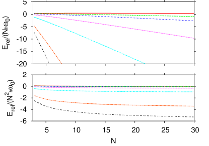
Figure 1: Top panel: Energies per particle for bosons confined on one dimension. The $y$-axis is stopped at -20 in order to show the general behaviour of many curves, though the shortest scattering lengths quickly leave the figure. The scattering lengths plotted, moving from bottom to top are 0.4., 0.5, 1.0, 2.0, 5.0, 10.0, and 100.0 Bottom panel: Energies divided by $N^{2}$ for the bosons to show their scaling behaviour with $N$. The order of the scattering lengths from bottom to is the same as in the top panel.

III Results

We now present numerical results for systems with $N=3-30$ particles, studying their energetics, the radial behaviour of the systems, and the one-body density matrix. Here we focus on the case of identical bosons. A particular issue is the ratio of the three-body energy to the two-body energy. An exact formula of MacGuire macguire1964 applies to one-dimensional systems of bosons with zero-range interactions and we make a comparison of the harmonic results to that model in the strongly-bound limit where the two-body energy is large and negative. Lastly, we consider also the thermodynamics of the system within the harmonic approximation.

III.1 Energies and radii

The ground state energy for bosons is shown in figure 1 and that for fermions in figure 2 for different particle numbers and scattering legnths. Notice that the upper panels show the energy per particle, while in the lower panels the energy is divided by a different power that we will discuss below. A striking feature to notice is the positivity of the energy for fermions, while that of the bosons can have both signs. This is a consequence of the Pauli principle which implies that the fermions will have to occupy higher orbitals for lack of degeneracies in one dimension as discussed above. Even in the case of very small scattering lengths (and thus large and negative two-body binding energies) the contribution from the higher orbits makes the overall ground state energy positive.

Once the two-body problem is solved and the parameters are determined, the ground state energy for bosons is given by (5). As seen in figure 1, the sign of the energy of the Bose system is mostly negative, but for small systems at large scattering lengths, the energy turns positive. This is understood from the fact that the energy shift, $V_{S}$, is negative and the shift term in the energy of (5) scales with $N^{2}$ while the positive oscillator frequency term scales with the lower power $N^{3/2}$. For bosons, the energy is positive for all particle numbers examined for $a/l=100$. Using (5), one can derive the critical number for bosons where the energy changes sign. It is given by

$$N_{crit}=\frac{\hbar^{2}\omega_{in}^{2}+2\hbar\sqrt{\hbar^{2}\omega_{in}^{4}/4+4V_{S}^{2}\omega_{0}^{2})}}{4V_{S}^{2}}.$$ (9)

From this relation one can calculate that for bosons the energy becomes negative at $a/l=100$ when $N\geq 116$.

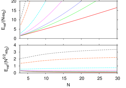
Figure 2: Top panel: Energies per particle for fermions confined on one dimension. The plotted scattering lengths are in the opposite order from the bosons as moves from the bottom to the top of the plot. Bottom panel: Fermion energies divided $N^{5/2}$ to clearly show the scaling of the energy with $N$.

The bottom panels of Figures 1 and 2 show the energies divided by the relevant scaling factor ($N^{2}$ for bosons and $N^{5/2}$ for fermions) to emphasize the scaling behaviour at large $N$. In the figures we can see that the asymptotic scalings are nicely approached when the scattering length is not too small. For the case of small scattering length, the two-body energy will in general behave as $E_{2}\sim-1/a^{2}$ while $\langle x^{2}\rangle\sim a^{2}$, since in this limit the trap can be ignored on the bound state branch in the spectrum that we study here. However, the relations in (3) and (4) that we use to determine our oscillator parameters now imply that both $V_{S}$ and $\omega_{in}$ must scale with $a^{-2}$ to be fulfilled (remember that $E_{2}$ is negative). This means that there will be a competition between the terms in the ground state energies given by (5) and (8). The asymptotic behaviour for large $N$ is therefore approached more slowly for small $a$.

We also calculate the relative size of the bosonic ground state wave functions, $\langle\left(X-X_{CM}\right)^{2}\rangle$, as a function of particle number for several different scattering lengths. Note here that $X$ denotes the single particle coordinate of one of the bosons and that no index is needed since the particles are identical. The results are shown in figure 3. One can see for the large scattering lengths that the radius increases before eventually decreasing for larger particle numbers (more than 20 for $a/l=100$). For scattering lengths of two and smaller, the size decreases monotonically with increasing particle number. Again this is connected to the fact that the small $a$ regime has very strong two-body binding and thus small $\langle x^{2}\rangle$ which is imprinted on the $N$-body system which tends to be very compact and presumably leads to strong clusterization in the real system followed by loss of atoms from the trap.

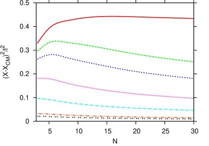
Figure 3: Radius $(x-X_{CM})^{2}$ for bosons as a function of particle number for several different scattering lengths. The scattering lengths are, from bottom to top, 0.4, 0.5, 1, 2, 5, 10, and 100.

For fermions (not shown), the Pauli principle and the subsequent need to occupy higher orbitals means that the system will in general be larger for the same scattering length and will not show a decreasing behaviour as $N$ is increased, but rather a slight increase. This can be seen from the energetics of the ground state in (8) which is dominated by the positive term containing the oscillator frequency for large $N$. This implies that the radius will stay large, constrained solely by the external trap.

We notice that the dimensional effect on the radius is quite clear when comparing to previous studies of bosonic systems in two and three dimensions arms11 . In the current one dimensional study, we see a non-monotonic behaviour in the radii as function of $N$ which can also be seen in two dimensions but which is almost completely absent in the corresponding three-dimensional system. The scattering lengths for which the maximum in the size occurs are roughly those where the three-body energy comes out positive. This implies an increased radial size, although still restricted by the external trapping potential. For large $N$, however, the bosons will always become negative in energy as the shift term dominates in (5) and the radius goes down again. The fact that lower dimensions show a more pronounced non-monotonicity of the size can then be traced to the fact that the positive energy contribution from zero-point motion grows with dimension and washes out the behaviour. For fermions, as discussed above, the energy is positive from the start and the radius stays large. However, the degeneracies allowed in higher dimensions adds extra ingredients and shell-structure to both energy and to the radial size.

III.2 Three boson energies

We now consider the case of three bosons within our harmonic approximation scheme in order to make a comparison to the results obtained by MacGuire macguire1964 in the absence of external confinement. The exact bound state energy, $E_{N}$, of $N$ bosons interacting via attractive pairwise zero-range interactions in a homogeneous one-dimensional space can be expressed in term of the two-body energy, $E_{2}$, as

$$E_{N}=\frac{1}{6}N\left(N^{2}-1\right)E_{2}.$$ (10)

For the case of three particles this becomes $E_{3}=4E_{2}$. Since we have an external trap, we do not expect to reproduce this result. However, in the limit $a\to 0$ where $E_{2}\to-\infty$ the external trap should become negligible and a comparison can be made.

We plot the ratio $E_{3}/E_{2}$ as a function of scattering length in figure 4 and as a function of $E_{2}$ in figure 5. The plot ends at $a/l\sim 0.25$ at which point it becomes numerically very challenging to compute the wave function based on the exact solution of Busch et al. busc98 . However, beyond that we can use the exact solution as discussed below.

One can see in figure 4 as the scattering length decreases (more clearly seen as $E_{2}\to-\infty$ in figure 5), that the ratio approach a limit. Using (5) and (4) in the limit where $a\to 0$ and $\omega_{r}\to\omega_{in}$ (see (6)), we get that

$$\frac{E_{3}}{E_{2}}=3+\left(\sqrt{\frac{3}{2}}-\frac{3}{2}\right)\frac{\omega_{in}}{E_{2}}.$$ (11)

Relating $\omega_{in}$ to $\langle x^{2}\rangle$ through (3), we obtain

$$\frac{E_{3}}{E_{2}}=3+\left(\sqrt{\frac{3}{2}}-\frac{3}{2}\right)\frac{\hbar^{2}}{2\mu E_{2}\langle x^{2}\rangle}.$$ (12)

We can now use the exact wave function for a delta function potential in one dimension, $\psi(x)=Ae^{-\kappa x}$ where $\kappa=\sqrt{-2\mu E_{2}/\hbar^{2}}$, to obtain $\hbar^{2}/(2\mu E_{2}\langle x^{2}\rangle)=2$. Our limit thus becomes $E_{3}/E_{2}\approx 3.55$. This is also the number we find numerically for the smallest value of $a$ that we could access. Comparing to the exact value of MacGuire, $E_{3}/E_{2}=4$, this implies that the energetics of our model is accurate to around 10% for small scattering lengths. The wave function in the harmonic model is a gaussian which in the limit $a\to 0$ will tend to a delta function, similar to the exact solution, so we also expect the harmonic model to provide an accurate structural description in this limit.

On the other hand, when $a$ becomes very large (the unitarity limit) the trap plays an important role. Looking back at the basic Hamiltonian in (1), we see that when $a\to\infty$, the interaction term tends to zero and we should be dominated by the trap only. However, the exact result does show that there is a shift of the energy in this limit so that $E_{2}=\hbar\omega/2$ for $a\to\infty$ (the non-interacting system has twice the energy since there is zero-point motion from both particles). Within our model we have $\omega_{r}\to\omega_{0}$ and $\langle x^{2}\rangle\to l^{2}/2$ when $a\to\infty$ as the external field provides the only length scale left in the problem. We have

$$\frac{E_{3}}{E_{2}}=3-\frac{\hbar\omega_{0}}{2E_{2}},$$ (13)

and in the large $a$ limit, $E_{2}\to\hbar\omega_{0}/2$, so we obtain a limiting value of $E_{3}\to 2$. At $a/l=100$, we numerically obtain 1.98 for this ratio so we reproduce this limit. The wave function becomes essentially exact in this limit, and we thus expect the structure to be well reproduces also.

In the limit of large $N$, we can also estimate the scalings and compare to the exact results when $a\to 0$. From (5) we have that the bosons scale as $E_{N}\sim N(N-1)E_{2}$, which means that we have an underbinding by a factor of $N+1$. Fermions in (8) are different since here we have $E_{N}\sim N^{5/2}E_{2}$, i.e. the underbinding is only by a factor of about $\sqrt{N}$. Notice, however, that in the opposite limit of $a\to\infty$, the dominant term in (5) and (8) change as $V_{S}\to 0$ and $\omega_{r}\to\omega_{0}$. This is an essentially non-interacting situation and we have the intuitively obvious result $E_{N}\sim N\hbar\omega_{0}/2$, which is just the scaling dictated by the trap. For values of $a$ away from these two limits, the scaling is an interplay of both terms and we get a more complicated behaviour. We note that one could also turn these arguments upside down and use the exact results for $N$ particles in the $a\to 0$ limit to fit the parameters of the model, for instance by using $E_{3}=4E_{2}$ instead of either the frequence of radius condition we impose on the two-body problem. Overall, we expect this to provide only minor quantitative changes in the harmonic model and its predictions.

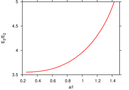
Figure 4: The ratio $E_{3}/E_{2}$ as a function of scattering length for bosons. We plot only the cases where both $E_{3}$ and $E_{2}$ are negative.

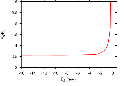
Figure 5: The ratio $E_{3}/E_{2}$ as a function of $E_{2}$ for bosons. We plot only the cases where both $E_{3}$ and $E_{2}$ are negative.

III.3 One-body density

The one body density matrix

$$\rho(x_{1},x_{1}^{\prime})=N\int\psi^{*}(x_{1},\dots,x_{N})\psi(x_{1}^{{}^{\prime}},\dots,x_{N})dx_{2}\dots dx_{N},$$ (14)

is the most basic correlation function and is the starting point of statistical property calculations. It contains information about the mean-field nature of the wave function for a bosonic system. It is of interest in itself, but we will focus on its largest eigenvalue, $\lambda$, which directly measures how much a given state has the structure of a coherent state. Figure 6 shows $\lambda$ as a function of the number of bosons for several scattering lengths. We mainly see an increase with particle number, though there are slight decreases for small particle numbers and large scattering lengths. In contrast with our previous results in arms11 for higher dimensions, only scattering lengths of order unity or smaller show a $\lambda$ much different than one, showing that the persistence of the mean-field structure provided by the external potential is quite strong in one dimension implying that the mean-field approximation is very good. The difference to higher dimensions arise from the degeneracies and from the reduction implied by the fact that one can factorize $\lambda$, so that for instance $\lambda_{3D}=\lambda^{3}$ (see arms11 ).

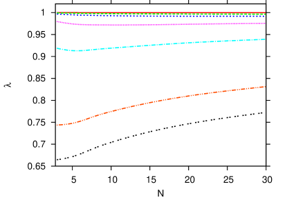
Figure 6: The value of $\lambda$ at several values of the 1D scattering length. From bottom to top they are 0.4, 0.5, 1, 2, 5, 10, and 100.

III.4 Thermodynamics

The energy spectrum can be obtained by considering center-of-mass excitations in the system and also the internal excitations characterized by the frequency in (6). To address the thermodynamics of the systems, one can proceed as described in detail in arms12 . One naturally starts with the partition function

$$Z(T)=\sum_{i}g_{i}\exp[-E_{i}/(k_{B}T)],$$ (15)

where $E_{i}$ is the energy of the $i$th state, $g_{i}$ is the degeneracy of that state, and $k_{B}$ is Boltzmann’s constant. 1D systems are simpler since there is no degeneracy in the energy levels in contrast to higher dimensions. With the sequence of energies and single-particle degeneracies, thermodynamic quantities can be calculated. Once the spectrum and degeneracies of our systems have been worked out, we can calculate basic thermodynamic quantities in the canonical ensemble. In 1D, the number of states grows much more slowly than in higher dimensions, though one does have to climb somewhat high in the spectrum due to the lack of degeneracy. In fact, in 1D there is no difference between bosons and fermions in the sequence of the degeneracies of the $N$-body excited states. This comes from the fact that all the Pauli principle implies for fermions is that the ground state has them occupying higher orbit which increases the ground state energy in comparison to bosons which can all go into the lowest orbital. Excitations on top of these ground states will now cost the same amount of energy and they will all have the same degeneracy since it is simply a matter of distribution of a number of particles in levels to obtain a specific total energy cost (the energy of the excitation above the ground state).

This latter fact implies that some thermodynamic quantities such as the entropy and heat capacity are identical for bosons and fermions at the same scattering length. Working in the canonical ensemble, in figure 7 we show the heat capacity $C$, which is the same for bosons and fermions. The heat capacity is related to the partition function by

$$C=\frac{\partial E}{\partial T},$$ (16)

$$E=-k_{B}T^{2}\frac{\partial\log Z}{\partial T}.$$ (17)

For all particle numbers, we see an initial increase, which then slows down at higher temperatures. This initial increase is the saturation of the center of mass mode. The temperature, where the slope changes, depends on particle number since more particles present in the system implies that the center of mass mode comprises a smaller share of the overall excitation energy. At the larger scattering lengths, the heat capacity then gradually increases towards the equipartion limit value of one. At small scattering lengths, the large size of the excitation frequency sharply delays the approach to the equipartition limit. For the same scattering length, more particles mean a slower approach to the high temperature limit. This is clear from (6), which shows that the excitation frequency increases with particle number.

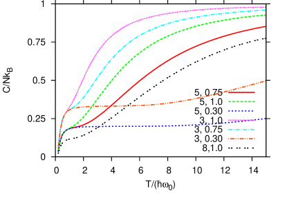
Figure 7: The heat capacity per particle at several boson numbers and scattering lengths, identified as $N,a$, as a function of temperature.

IV Summary and outlook

We have presented results for an $N$-body system of particles moving in one dimension and interacting via pairwise zero-range interactions under the influence of an external harmonic oscillator trap. The Hamiltonian is solved analytically within the harmonic approximation where the parameters of the model are adjusted to reproduce properties of the exact solution of the corresponding two-body problem. This is along the lines of the standard approach to many-body problems in many fields of physics.

The ground state energies for both bosonic and fermionic systems were determined and we discussed the scaling of these quantities with the particle number. We also obtained the radial size of the bosonic systems and compared to previous findings in two- and three-dimensional setups. A careful study of the energy of three bosons in the harmonic model reveals that in the limit of large two-body binding energy where the external trap can be neglected, the harmonic model results are about 10% below the exact result abtained by MacGuire macguire1964 , while in the opposite limit of negligible two-body binding energy (large scattering length) the model becomes essentially exact. For larger particle numbers, the harmonic approximation tends to underbind the system compared to the exact results when the two-body system is strongly bound.

Additionally, we studied the one-body density matrix. The main goal was the computation of its largest eigenvalue to characterize the degree of coherence in the system. The results turn out to be similar to those obtained in two and three dimensions, except that the one-dimensional coherence turns out to be more robust except for large two-body binding energies. Lastly, we studied the thermodynamics of the one-dimensional system. The specific heat was found to behave in a manner that is also quite similar to higher dimensions. However, it is worth noticing that within the harmonic model, the spectrum of excitation for bosons and fermions turns out to be exactly the same. Due to the lack of degeneracy of the levels in one dimensions, the only difference is therefore found in the ground state energy.

The one-dimensional setup studied here provides a very valuable benchmark for the harmonic models that have been used in higher dimensions in different contexts calogero1971 ; zaluska2000 ; yan2003 ; gajda2006 . Another good test ground for the harmonic models is systems that have long-range interaction. In particular, systems of dipolar molecules in one-dimensional tubes have been studied recently due to their interesting few- and many-body structure arguelles2007 ; kollath2008 ; chang2009 ; huang2009 ; wunsch2011 ; dalmonte2011 ; zinner2011 ; fellows2011 ; knap2012 ; leche2012 . The dipole-dipole interaction in two different one-dimensional tubes is typically characterized by having a pocket which becomes deep when the dipolar interaction is strong zinner2011 . This implies that a harmonic approximation is a good starting point. This approach has been studied in the case of two-dimensional layers with dipolar particles wang2006 ; jeremy2010 ; zinner2011d ; jeremy2011 and compares very well to exact results artem2011a ; artem2011b ; artem2012 away from the weak-coupling limit. The application of the harmonic approximation to one-dimensional arrays containing dipolar particles is a topic for future work.

Another interesting direction in which the harmonic model can be used is for the study of higher-order terms in the interaction such as those coming from effective-range corrections to the model of Busch et al. busc98 ; zinner2012 . Recent experiments have shown a potential need for such corrections in both two- baur2012 and three-dimensional cold atomic gas systems ohara2012 . A possible way to account for such corrections would be to include quartic interaction terms an then carefully fit the additional parameter to few-body properties. Within the harmonic model, the quartic interactions can be computed quite straightforwardly through gaussian integrals. This could then be compared to mean-field results that include effective-range corrections in the limit of large particle numbers fu2003 ; zinner2009a ; zinner2009b ; thoger2009 .

References

- (1) Mattis D 1993 The Many-Body Problem (Singapore: World Scientific)
- (2) Sutherland B 2004 Beautiful Models (Singapore: World Scientific)
- (3) Bethe H 1931 Z. Physik 71 205
- (4) Lieb E H and Liniger W 1963 Phys. Rev. 130 1605
- (5) Lieb E H 1963 Phys. Rev. 130 1616
- (6) MacGuire J 1964 J. Math. Phys. 5 622
- (7) Sutherland B 1971 J. Math. Phys. 12 246
- (8) Calogero F 1971 J. Math. Phys. 12 419
- (9) Bloch I, Dalibard J and Zwerger W 2008 Rev. Mod. Phys. 80 885
- (10) Parades B, Widera A, Murg V, Mandel O, Fölling S, Cirac I, Shlyapnikov G V, Hänsch T W and Bloch I 2004 Nature 429 277
- (11) Kinoshita T, Wenger T and Weiss D S 2004 Science 305 1125
- (12) Haller E, Gustavsson M, Mark M J, Danzl J G, Hart R, Pupillo G and Nägerl H-C 2009 Science 325 1224
- (13) Tonks L 1936 Phys. Rev. 50 955
- (14) Girardeau M 1960 J. Math. Phys. 1 516
- (15) Serwane F, Zürn G, Lompe T, Ottenstein T B, Wenz A N and Jochim S 2011 Science 332 6027
- (16) Zürn G, Serwane F, Lompe T, Wenz A N, Ries M G, Bohn J E and Jochim S 2012 Phys. Rev. Lett. 108 075303
- (17) Armstrong J R, Zinner N T, Fedorov D V and Jensen A S 2011 J. Phys. B 44 055303
- (18) Busch T, Englert B-G, Rzażewski K and Wilkens M 1998 Found. Phys. 28 549
- (19) Farrell A and van Zyl B J. Phys. A 2010 43 015302
- (20) Armstrong J R, Zinner N T, Fedorov D V and Jensen A S 2012 Phys. Rev. E 85 021117
- (21) Olshanii M 1998 Phys. Rev. Lett. 81 938
- (22) Yang C N 1962 Rev. Mod. Phys. 34 694
- (23) Zaluska-Kotur M A, Gajda M, Orlowski A and Mostowski J 2000 Phys. Rev. A 61 033613
- (24) Yan J 2003 J. Stat. Phys. 113 623
- (25) Gajda M 2006 Phys. Rev. A 73 023603
- (26) Argüelles A and Santos L 2007 Phys. Rev. A 75 053613
- (27) Kollath C, Meyer J S and Giamarchi T 2008 Phys. Rev. Lett. 100 130403
- (28) Chang C-M, Shen W-C, Lai C-Y, Chen P and Wang D-W 2009 Phys. Rev. A 79 053630
- (29) Huang Y-P and Wang D-W 2009 Phys. Rev. A 80 053610
- (30) Wunsch B, Zinner N T, Mekhov I B, Huang S-J, Wang D-W and Demler E 2011 Phys. Rev. Lett. 107 073201
- (31) Dalmonte M, Zoller P and Pupillo G 2011 Phys. Rev. Lett. 107 163202
- (32) Zinner, N T, Wunsch B, Mekhov I B, Huang S-J, Wang D-W and Demler E 2011 Phys. Rev. A 84 063606
- (33) Fellow J M and Carr S T 2011 Phys. Rev. A 84 051602(R)
- (34) Knap M, Berg E, Ganahl M and Demler E 2012 Phys. Rev. B 86 064501
- (35) Lecheminant P and Nonne H 2012 Phys. Rev. B 85 195121
- (36) Wang D-W, Lukin M D and Demler E 2006 Phys. Rev. Lett. 97 180413
- (37) Armstrong J R, Zinner N T, Fedorov D V and Jensen A S 2010 Europhys. Lett. 91 16001
- (38) Zinner N T, Armstrong J R, Volosniev A G, Fedorov D V and Jensen A S 2012 Few-Body Syst. 53 369
- (39) Armstrong J R, Zinner, N T, Fedorov D V and Jensen A S 2012 Eur. Phys. J. D 66 85
- (40) Volosniev A G, Fedorov D V, Jensen A S and Zinner N T 2011 Phys. Rev. Lett. 106 250401
- (41) Volosniev A G, Zinner N T, Fedorov D V, Jensen A S and Wunsch B 2011 J. Phys. B 44 125301
- (42) Volosniev A G, Fedorov D V, Jensen A S and Zinner N T 2012 Phys. Rev. A 85 023609
- (43) Zinner N T 2012 J. Phys. A 45 205302
- (44) Baur S K, Fröhlich B, Feld M, Vogt E, Perlot D, Koschorreck M and Köhl M 2012 Phys. Rev. A 85 061604(R)
- (45) Hazlett E L, Zhang Y, Stites R W and O’Hara K M 2012 Phys. Rev. Lett. 108 045304
- (46) Fu H, Wang Y and Gao B 2003 Phys. Rev. A 67 053612
- (47) Zinner N T and Thøgersen M 2009 Phys. Rev. A 80 023607
- (48) Zinner N T 2009 Preprint arXiv:0909.1314
- (49) Thøgersen M, Zinner N T and Jensen A S 2009 Phys. Rev. A 80 043625