Time-Varying Space-Only Codes for Coded MIMO

Abstract

Multiple antenna (MIMO) devices are widely used to increase reliability and information bit rate. Optimal error rate performance (full diversity and large coding gain), for unknown channel state information at the transmitter and for maximal rate, can be achieved by approximately universal space-time codes, but comes at a price of large detection complexity, infeasible for most practical systems. We propose a new coded modulation paradigm: error-correction outer code with space-only but time-varying precoder (as inner code). We refer to the latter as Ergodic Mutual Information (EMI) code. The EMI code achieves the maximal multiplexing gain and full diversity is proved in terms of the outage probability. Contrary to most of the literature, our work is not based on the elegant but difficult classical algebraic MIMO theory. Instead, the relation between MIMO and parallel channels is exploited. The theoretical proof of full diversity is corroborated by means of numerical simulations for many MIMO scenarios, in terms of outage probability and word error rate of LDPC coded systems. The full-diversity and full-rate at low detection complexity comes at a price of a small coding gain loss for outer coding rates close to one, but this loss vanishes with decreasing coding rate.

I Introduction

Multiple antennas (MIMO) has become an important means to combat channel fading as well as to increase channel capacity. Since the pioneering work [25, 42], a great amount of research effort has been focused on characterizing the fundamental limits of MIMO communications that are now well understood in many aspects. In particular, when the channel is subject to slow fading, a fundamental tradeoff as to how to optimally exploit the multiple antennas has been characterized in [52].

Code design problems for multi-antenna channels without channel state information at the transmitter have first been addressed by Tarokh et al. in [40], in which the notion of space-time codes was introduced. By spanning the message over both spatial and temporal dimensions, full spatial diversity can be achieved. The elegant construction of orthogonal space-time codes enables a simple decoding at the receiver side [40, 2]. Unfortunately, the benefit of simplicity is obtained at the cost of rate; more specifically, at most one independent symbol per channel use can be transmitted. Furthermore, the rate of orthogonal space-time codes decreases with the number of transmit antennas, while the ergodic capacity of a MIMO channel linearly increases with the minimum of the number of receive and transmit antennas. While the highly structured codes have a poor spectral efficiency, the random coding argument [52, 18] suggests that there exists a space-time code with finite length that can achieve the fundamental diversity-multiplexing tradeoff (DMT). Guided by the diversity-multiplexing tradeoff, approximately universal [41], i.e., DMT optimal for all channel statistics, structured space-time codes designs have been proposed [4, 19, 20, 41]. The key to obtain approximately universal space-time codes with a finite code length is the non-vanishing properties of the product of the $\min\{n_{T},{n_{R}}\}$ smallest singular values of the codeword matrices for increasing signal-to-noise ratio, where $n_{T}$ and ${n_{R}}$ are the number of transmit and receive antennas, respectively. In particular, this criterion coincides with the non-vanishing determinant criterion when $n_{T}={n_{R}}$ [19, 20]. Interestingly enough, when the MIMO channel is diagonal, i.e., a parallel channel, the criterion is reduced to the product-distance criterion, well known for code design for single-antenna block fading channels [6, 3, 44].

In general, the MIMO channel can be decomposed by the singular value decomposition into a diagonal channel preceded by a random unitary matrix rotating the channel input. Despite the diagonal channel being present in the singular value decomposition, there is a fundamental difference between MIMO and parallel channels when the channel state is unknown at the transmitter side. In fact, by carefully examining the criterion for approximate universality [41, 20], constraints on the codeword structure are imposed in order to guarantee a “good” performance for the worst-case rotation incurred by the channel matrix. Such a phenomenon does not exist for diagonal/parallel channels. To guarantee good performance in any MIMO channel, precoding over at least $n_{T}^{2}$ dimensions is needed for MIMO, while we only need to code over $n_{T}$ dimensions for parallel channels. A direct consequence of the increased precoding dimensionality is the decoding complexity. While there exist efficient decoding algorithms for such problems (see [28, 34] and references therein), the complexity still grows in polynomial time with the dimension for the best-case scenarios and in exponential time for the worst cases.

The advantages of approximately universal space-time code designs are quite clear: high spectral efficiency, high diversity gains even without channel codes, and short block length. On the other hand, error-correction codes with relatively large block lengths are used in most modern communication systems. As a result, a common paradigm of coding for multi-antenna systems is the concatenation of an error correction code (also referred to as outer code) and a space-time code (also referred to as space-time precoder, or inner code). That is, a long coded block is split into many sub-blocks that are space-time precoded individually. While the precoder is designed without the consideration of an outer channel code, the actual error performance depends on multiple space-time blocks. Although using a well-designed space-time precoder can only improve the overall error rate performance, it comes at the price of high decoding complexity, as mentioned above. In fact, it turned out in some cases that the use of space-time codes in conjunction with channel codes does not bring extra gain but unnecessary decoding complexity (e.g. when the coding rate of the channel code is sufficiently low to recover a portion of the spatial diversity [26]). Therefore, the conventional paradigm, to design space-time codes without considering the presence of an outer code, may not be efficient when it comes to the trade-off between performance and complexity.

Inspired by the connection between MIMO and parallel channels (the MIMO channel is a parallel channel with random precoder) as well as the observation that the outer codeword spans over a large amount of channel uses, we propose a new coded modulation paradigm: error correction codes with space-only but time-varying precoder. The rationale behind this is to avoid the worst-case rotations (denoted as corrupt precoders in this paper) that are the main factor of deterioration in uncoded MIMO communication. The time-varying aspect of the space-only precoder reduces the effect of the worst-case rotations to a fraction of the transmission time, which can then be compensated by the outer code. Note that space-only precoders have been considered in the literature when channel state information was available at the transmitter (e.g. through feedback), see [31] and references therein.

The main contribution of this paper is as follows. We first observe that the MIMO channel corresponds to a parallel channel with a precoder that is random, but then remains fixed once it is chosen. We then extend the framework of signal space diversity for parallel channels to explain why full transmit diversity is not achieved with fixed space-only codes for MIMO. This new framework allows us to prove Theorem 1, claiming that time-varying space-only precoders achieve full diversity on any MIMO channel, thereby proposing an alternative to approximately universal space-time codes with a much smaller detection complexity.

The rest of the paper is organized as follows. The system model, notation and problem statement are presented in Sec. II and we also clearly define what we mean by full-rate space-time codes. In Sec. III, we interpret MIMO as parallel channels with a random precoder and explain that this randomness requires an extension of the study on signal space diversity for parallel channels. We first illustrate this extension by means of a toy example in Sec. IV, where the channel gains, the precoder elements and the transmit symbols are all real-valued. Next, the extension of the signal space diversity framework is formalized in Sec. V, by introducing the concepts of bad and corrupt precoders. This new framework is then used to prove that fixed space-only codes do not achieve full diversity (Sec. VI) in contrary to time-varying space-only precoders (Sec. VII). Theorem 1 is then corroborated by presenting extensive numerical results in Sec. VIII.

II System model

Notation: we write scalars, vectors and matrices as $x$, $\mathbf{x}$ and $X$. $X^{\dagger}$ and $\mathbf{x}^{\dagger}$ are the Hermitian transposes of $X$ and $\mathbf{x}$. The Landau symbols $f(n)=O(g(n))$ and $f(n)=\Omega(g(n))$ respectively denote $f(n)\leq kg(n)$ and $f(n)\geq kg(n)$ for some positive $k$. The equation sign $f(\gamma)\doteq g(\gamma)$, introduced in [52], is equivalent to $\lim_{\gamma\rightarrow\infty}\frac{\log f(\gamma)}{\log\gamma}=\lim_{\gamma\rightarrow\infty}\frac{\log g(\gamma)}{\log\gamma}$. Similar meanings hold for $\dot{\leq}$ and $\dot{\geq}$.

II-A Channel model

We consider a point-to-point MIMO channel $H=[h_{i,j}]\in\mathbb{C}^{{n_{R}}\times n_{T}}$ with $n_{T}$ transmit antennas and ${n_{R}}$ receive antennas, where $h_{i,j}\sim\mathcal{C}\mathcal{N}(0,1)$ is the complex path gain from transmit antenna $j$ to receive antenna $i$. We assume that all path gains are independent. The channel state information is perfectly known at the receiver side, but unknown at the transmitter side, i.e., no feedback channel is available. The channel is assumed to vary slowly, so that it remains constant during the transmission of at least one outer codeword. A channel use is referred to as the event where the transmitter sends $n_{T}$ symbols simultaneously from its $n_{T}$ transmit antennas. Assuming a total of $N_{c}$ channel uses per codeword, the discrete-time complex baseband equivalent channel equation is given by

$$\mathbf{\tilde{y}}_{t}=\sqrt{\gamma}\,H\mathbf{\tilde{x}}_{t}+\mathbf{\tilde{w}}_{t},~{}~{}t=1,\ldots,N_{c},$$ (1)

where $\mathbf{\tilde{y}}_{t},\mathbf{\tilde{w}}_{t}\in\mathbb{C}^{{n_{R}}\times 1}$ denote the received vector and noise vector at instant $t$, and $\mathbf{\tilde{x}}_{t}\in\mathbb{C}^{n_{T}\times 1}$ denotes the symbol vector transmitted at instant $t$. The additive white Gaussian noise vector $\mathbf{\tilde{w}}_{t}$ has i.i.d. entries, $\tilde{w}_{t,i}\sim\mathcal{C}\mathcal{N}(0,1)$. The transmit vector $\mathbf{\tilde{x}}_{t}$ satisfies $\mathbb{E}[||\mathbf{\tilde{x}}_{t}||^{2}]=n_{T},\forall~{}t$. This way, $\gamma$ is the average signal-to-noise ratio per symbol (SNR) per transmit antenna. The instantaneous mutual information is denoted as $I(\mathbf{\tilde{x}}_{t};\mathbf{\tilde{y}}_{t}|H)$ and depends on the channel realization $H$.

The channel realization $H$ can be decomposed by a singular value decomposition as $H=U\Sigma V^{\dagger}$, where $U\in\mathbb{C}^{{n_{R}}\times{n_{R}}}$ and $V\in\mathbb{C}^{n_{T}\times n_{T}}$ are unitary matrices, uniformly distributed in the set of all unitary matrices (see App. -A for more background), and $\Sigma\in\mathbb{R}^{{n_{R}}\times n_{T}}$ is a diagonal matrix with the non-negative singular values $\sigma_{i},i=1,\ldots,\min({n_{R}},n_{T}),$ of $H$ on its diagonal. As in [52, 22], we define the ordered normalized fading gains $\boldsymbol{\alpha}=[\alpha_{1},\ldots,\alpha_{\min({n_{R}},n_{T})}]$, where $\alpha_{i}=-\frac{\log\sigma_{i}^{2}}{\log\gamma}$, $\alpha_{1}\geq\alpha_{2}\geq\ldots\geq\alpha_{\min({n_{R}},n_{T})}$. The joint distribution $p(\boldsymbol{\alpha})$ is given by [52, 33]

$$p(\boldsymbol{\alpha})=K^{-1}(\log{\gamma})^{n_{T}}\prod_{i=1}^{\min({n_{R}},n_{T})}\gamma^{-(|{n_{R}}-n_{T}|+1)\alpha_{i}}$$

$$\prod_{j>i}(\gamma^{-\alpha_{i}}-\gamma^{-\alpha_{j}})^{2}e^{-\sum_{i=1}^{\min({n_{R}},n_{T})}\gamma^{-\alpha_{i}}}.$$ (2)

Because $H$ is known at the receiver, the following transformation can be performed,

$$\mathbf{y}_{t}=U^{\dagger}\mathbf{\tilde{y}}_{t}=\sqrt{\gamma}~{}\Sigma V^{\dagger}\mathbf{\tilde{x}}_{t}+\mathbf{w}_{t},\quad t=1,\ldots,N_{c}$$ (3)

where $\mathbf{w}_{t}$ follows the same distribution as $\mathbf{\tilde{w}}_{t}$. Because the transformation matrix $U^{\dagger}$ is invertible, no information is lost by this transformation (which can be proved by for example the data processing inequality [10]) , i.e., $I(\mathbf{\tilde{x}}_{t};\mathbf{y}_{t}|\Sigma,V)=I(\mathbf{\tilde{x}}_{t};\mathbf{\tilde{y}}_{t}|H)$.

Let us now consider (3) in the cases ${n_{R}}>n_{T}$ and ${n_{R}}<n_{T}$, where $\Sigma$ is not square. When ${n_{R}}>n_{T}$ and $\Sigma$ is tall, the last ${n_{R}}-n_{T}$ received symbols in $\mathbf{y}_{t}$ contain only noise due to the fact that the bottom ${n_{R}}-n_{T}$ rows of $\Sigma$ are zero. Hence, when we consider ${n_{R}}>n_{T}$ in the following, then, allowing an abuse in notation, $\mathbf{y}_{t}$, $\mathbf{w}_{t}$ and $\Sigma$ refer to the top $n_{T}$ rows of the actual vectors $\mathbf{y}_{t}$, $\mathbf{w}_{t}$ and $\Sigma$, respectively. As a result, an equivalent $n_{T}\times n_{T}$ MIMO channel is obtained, of course taking into account the actual singular value distribution as a function of ${n_{R}}$ and $n_{T}$ (see (2)). When ${n_{R}}<n_{T}$ and $\Sigma$ is fat, the last $n_{T}-{n_{R}}$ columns of $\Sigma$ are zero, so that the last $n_{T}-{n_{R}}$ columns of $V$ are not important, which will be considered in Sec. VII.

The outage probability [5, 37] is expressed as

$$P_{\textrm{out}} =\textrm{Pr}\left(\left[\lim_{N_{c}\rightarrow\infty}\frac{1}{N_{c}}\sum_{t=1}^{N_{c}}I(\mathbf{\tilde{x}}_{t};\mathbf{y}_{t}|\Sigma,V)\right]<R\right)$$ (4)

$$=\textrm{Pr}\left(\mathbb{E}_{t}\left[I(\mathbf{\tilde{x}}_{t};\mathbf{y}_{t}|\Sigma,V)\right]<R\right),$$ (5)

where $R$ is the spectral efficiency and $\mathbb{E}_{t}\left[.\right]$ denotes the temporal mean. The SNR-exponent of the outage probability, known as the diversity order, is

$$d_{\textrm{out}}=\lim_{\gamma\rightarrow\infty}-\frac{\log P_{\textrm{out}}}{\log\gamma},$$ (6)

where we assumed fading distributions where the limit in (6) exists.

II-B Full rate space-time and space-only coding

In this paper, full-rate STCs are considered where we define full-rate codes as schemes that transmit, on average, a linear transformation of $\min(n_{T},{n_{R}})$ independent $M$-QAM symbols at each channel use, corresponding to $m$ coded bits per channel use, where $m=\min(n_{T},{n_{R}})\log_{2}M$. Hence, the number of channel uses per codeword is $N_{c}=\frac{N_{b}}{m}$, where $N_{b}$ is the length of a codeword of the outer code.

Note that it is possible to convey $n_{T}$ independent symbols per channel use, which is larger than $\min(n_{T},{n_{R}})$ when ${n_{R}}<n_{T}$. However, transmitting $\min(n_{T},{n_{R}})$ independent symbols maximizes the multiplexing gain (the speed at which the constellation size may grow with the SNR $\gamma$) that can be achieved without leading to a degradation of the error rate for increasing SNR [52]. Secondly, the capacity of an $n_{T}\times{n_{R}}$ MIMO channel is the same as the capacity of an ${n_{R}}\times n_{T}$ MIMO channel (hence with ${n_{R}}$ transmit antennas and $n_{T}$ receive antennas) [47, 24, 42], so that transmitting more symbols on the $n_{T}\times{n_{R}}$ MIMO channel than the maximum that can be conveyed on the ${n_{R}}\times n_{T}$ MIMO channel would not correspond to the limits of the channel, and thus lead to a significant loss in coding gain.

STCs are characterized by the number of space and time dimensions, $n_{T}$ and $k$, respectively, denoted as an $n_{T}\times k$ STC. When the number of time dimensions $k$ reduces to one, the STC becomes a space-only code. An $n_{T}\times k$ STC (consisting of $n_{T}k$ elements) yields $k$ symbol vectors $\{\mathbf{\tilde{x}}_{(l-1)k+1},\ldots,\mathbf{\tilde{x}}_{(l-1)k+k}\}$, often represented through an $n_{T}\times k$ STC matrix $X_{l}$, where $X_{l,u,i}=\tilde{x}_{(l-1)k+u,i},i=1,\ldots,n_{T};u=1,\ldots,k;l=1,\ldots,N_{c}/k$.

We first consider the case that ${n_{R}}\geq n_{T}$. The STC $X_{l}$ is obtained from $mk$ coded bits through a sequence of operations. The sequence of $mk$ coded bits is split in $n_{T}k$ groups of $m/n_{T}$ bits which are mapped to one of $M$ points, $M=2^{m/n_{T}}$, belonging to an $M$-QAM constellation $\Omega_{z}$. Denoting as $\mathbf{z}_{l}$ the $n_{T}k$-dimensional symbol vector that results from mapping the $l$-th block of $mk$ coded bits, the linear precoding involves

$$\mathbf{\tilde{x}}_{\textrm{vec},l}=P_{l}\mathbf{z}_{l},~{}l=1,\ldots,N_{c}/k,$$ (7)

where $P_{l}$ is a well chosen unitary matrix in $\mathbb{C}^{nk\times nk}$ and $\mathbb{E}[|z_{l,j}|^{2}]=1,j=1,\ldots,n_{T}k$. Next, the $n_{T}k$-dimensional vector $\mathbf{\tilde{x}}_{\textrm{vec},l}$ is split in $k$ column vectors of length $n_{T}$, yielding the STC matrix $X_{l}$ or the $k$ vectors $\{\mathbf{\tilde{x}}_{(l-1)k+1},\ldots,\mathbf{\tilde{x}}_{(l-1)k+k}\}$. Because $\mathbb{E}[|z_{l,j}|^{2}]=1$ and $P_{l}$ is unitary, the components $\tilde{x}_{t,i}$ satisfy $\mathbb{E}[|\tilde{x}_{t,i}|^{2}]=1,\forall~{}i,t$.

In the case that ${n_{R}}<n_{T}$, full-rate codes transmit, on average, a linear transformation of ${n_{R}}$ independent $M$-QAM symbols each channel use. Hence, $\mathbf{z}_{l}$ only contains ${n_{R}}k$ independent components. For example, $(n_{T}-{n_{R}})k$ components of $\mathbf{z}_{l}$ can be put to zero. To satisfy the constraint that $\mathbb{E}[||\mathbf{\tilde{x}}_{t}||^{2}]=n_{T},\forall~{}t$, we set the mean square magnitude of the ${n_{R}}k$ non-zero components of $\mathbf{z}_{l}$ equal to $\frac{n_{T}}{{n_{R}}}$.

II-C Problem formulation

The approximately universal STCs that are optimal in terms of uncoded error rate for an $n_{T}\times{n_{R}}$ MIMO channel are $n_{T}\times n_{T}$ full-rate full-diversity STCs (hence $k=n_{T}$). The precoder $P_{l}=P$ is constant, has dimension $n_{T}^{2}\times n_{T}^{2}$ and its $n_{T}^{4}$ elements are optimized to maximize the coding gain (see for example [4, 30, 36, 40, 26, 8]). A prohibitive objection is that the detection complexity of optimal STCs is very complex, e.g., it increases exponentially with $n_{T}^{2}$ for exhaustive ML-detection. For example, when $16-$QAM and $n_{T}=3$ transmit antennas are used, the detection complexity is $O(16^{9})$. Although a recent study shows that the complexity of near-ML decoding can be reduced to growing in polynomial time with the dimension for the best-case scenarios, by using lattice reduction and linear preprocessing [28], it is yet to be verified whether the same conclusion holds with error correcting codes and soft decoding.

We propose full-rate time-varying space-only codes, hence $k=1$ so that $P_{l}$ only has dimension $n_{T}\times n_{T}$, but $P_{l}$ varies with $l$. In Sec. VII, we prove that full diversity is achieved. Because the STC is space-only, the notation simplifies: $\mathbf{\tilde{x}}_{t}=P_{t}\mathbf{z}_{t}$, $t=1,\ldots,N_{c}$, where $z_{t,i}\in\Omega_{z}$, $i=1,\ldots,\min(n_{T},{n_{R}})$. Hence, $\mathbf{z}_{t}$ belongs to $\Omega_{\mathbf{z}}=(\Omega_{z})^{n_{T}}$, which is the Cartesian product of $n_{T}$ constellations $\Omega_{z}$. We denote our new precoder type by the EMI code, where EMI (Ergodic Mutual Information) refers to the temporal mean of the mutual information. The detection complexity of exhaustive ML-detection now increases exponentially with $\min(n_{T},{n_{R}})$ which is the lowest possible ML detection complexity for full-rate STCs. For example, when $\Omega_{z}=16-$QAM and $n_{T}={n_{R}}=3$, the detection complexity is $O(16^{3})$ for exhaustive ML-decoding, which is feasible.

The overall received signal-to-noise ratio per information bit is denoted as $\frac{E_{b}}{N_{0}}$, where $E_{b}$ is the ratio of the energy of the received symbol vector and the number of information bits conveyed per transmitted symbol vector, so that $\frac{E_{s}}{N_{0}}=\gamma=\frac{RE_{b}/N_{0}}{\mathbb{E}[||\mathbf{\tilde{x}}_{t}||^{2}]{n_{R}}}$, where $R=mR_{c}$ is the spectral efficiency and $R_{c}$ is the coding rate. When the constraint $\mathbb{E}[||\mathbf{\tilde{x}}_{t}||^{2}]=n_{T},\forall~{}t$, is satisfied, then the SNR is $\gamma=\frac{RE_{b}/N_{0}}{n_{T}{n_{R}}}$.

III MIMO vs. parallel channels

The channel equation (3) is that of a parallel channel $\Sigma$ (which corresponds to $\min(n_{T},{n_{R}})$ parallel channels), with precoded input $V^{\dagger}\mathbf{\tilde{x}}_{t}$, with the particular feature that the precoder $V^{\dagger}$ is random. We denote the input of this parallel channel by

$$\mathbf{x}_{t}=V^{\dagger}\mathbf{\tilde{x}}_{t},$$ (8)

which belongs to a discrete constellation that is random (through $V$) and variable in time (through the time-varying precoder $P_{t}$). Allowing a small abuse in notation (by dropping the time-index), we denote this constellation by $\Omega_{\mathbf{x}}$, so that $\mathbf{x}_{t}\in\Omega_{\mathbf{x}}$. It is clear that $\mathbf{x}_{t}$ is a linear transformation of $\mathbf{z}_{t}$,

$$\mathbf{x}_{t}=V^{\dagger}P_{t}\mathbf{z}_{t}=V_{t}\mathbf{z}_{t},$$ (9)

where the precoder $V_{t}=V^{\dagger}P_{t}$ is random and varies in time within the duration of a codeword if $P_{t}$ is time-varying. When $P_{t}$ is deterministic or uniformly distributed in the set of all unitary matrices (denoted as $\mathcal{M}(n_{T},n_{T})$) and independent from $V$, then $V_{t}$ is also uniformly distributed in $\mathcal{M}(n_{T},n_{T})$ (see Lemma 5 in App. -A). Hence, in the case that a fixed space-only precoder $P_{t}=P$ is used, the MIMO channel corresponds to a parallel channel with a random precoder $V^{\dagger}P$, and when our proposed time-varying space-only precoder $P_{t}$ is used, the MIMO channel corresponds to a parallel channel with a random time-varying precoder $V_{t}$.

For a given channel realization and a given channel use, $\Omega_{\mathbf{x}}$ is fixed and we can determine the mutual information between input and output of this parallel channel, $I(\mathbf{x}_{t};\mathbf{y}_{t}|\Sigma,V)=I(\mathbf{\tilde{x}}_{t};\boldsymbol{y}_{t}|H)$. Inserting $\mathbf{x}_{t}$ in Eq. (3), we have that

$$\mathbf{y}_{t}=\sqrt{\gamma}~{}\Sigma\mathbf{x}_{t}+\mathbf{w}_{t},\quad t=1,\ldots,N_{c},$$ (10)

Note that only the top $\min(n_{T},{n_{R}})$ components of the column vector $\mathbf{x}_{t}$ are important, by the structure of $\Sigma$; hence, the complete vector $\mathbf{x}_{t}$ is considered when ${n_{R}}\geq n_{T}$, and the top ${n_{R}}$ components of $\mathbf{x}_{t}$ otherwise.

The mutual information $I(\mathbf{x}_{t};\mathbf{y}_{t}|\Sigma,V)$ between input and output of a parallel channel is well known [45, 22] and recalled in Eq. (12), where $d^{2}(\mathbf{c},\mathbf{d})=\sum_{i=1}^{n_{T}}|c_{i}-d_{i}|^{2}$. Using the normalized fading gains, the mutual information can be expressed as in Eq. (13), where

$$f(\alpha_{i},s_{t,i},w_{t,i})=e^{-\gamma^{1-\alpha_{i}}|s_{t,i}|^{2}-2\sqrt{\gamma^{1-\alpha_{i}}}\mathcal{R}\{w_{t,i}s_{t,i}^{*}\}},$$ (11)

and where $s_{t,i}=(x_{t,i}-x_{t,i}^{\prime})$ and $\mathcal{R}\{.\}$ takes the real part.

$$I\left(\mathbf{x}_{t};\mathbf{y}_{t}|\Sigma,V\right) =m-2^{-m}\sum_{\mathbf{x}_{t}\in\Omega_{\mathbf{x}}}\mathbb{E}_{\mathbf{y}_{t}|\mathbf{x}_{t}}\left[\textrm{log}_{2}\left(\sum_{\mathbf{x}_{t}^{\prime}\in\Omega_{\mathbf{x}}}\exp\left[\left(d^{2}(\mathbf{y}_{t},\sqrt{\gamma}\Sigma\mathbf{x}_{t})-d^{2}(\mathbf{y}_{t},\sqrt{\gamma}\Sigma\mathbf{x}_{t}^{\prime})\right)\right]\right)\right]$$ (12)

$$=m-2^{-m}\sum_{\mathbf{x}_{t}\in\Omega_{\mathbf{x}}}\mathbb{E}_{\mathbf{w}_{t}}\left[\textrm{log}_{2}\left(\sum_{\mathbf{x}_{t}^{\prime}\in\Omega_{\mathbf{x}}}\prod_{i=1}^{n_{T}}f(\alpha_{i},s_{t,i},w_{t,i})\right)\right]$$ (13)

The parallel channel model with precoding is well known for the study of signal space diversity (SSD) (see [6] for uncoded and [23, 13] for coded communication over parallel channels). In SSD, full transmit diversity is achieved when $V_{t}$ is chosen so that $s_{t,i}\neq 0,i=1,\ldots,\min(n_{T},{n_{R}}),\forall~{}t$, where $\mathbf{s}_{t}=\mathbf{x}_{t}^{\prime}-\mathbf{x}_{t};~{}\mathbf{x}_{t}^{\prime}=V_{t}\mathbf{z}^{\prime},\mathbf{x}_{t}=V_{t}\mathbf{z};\mathbf{z},\mathbf{z}^{\prime}\in\Omega_{\mathbf{z}}$, $\mathbf{z}^{\prime}\neq\mathbf{z}$. Mostly, the fading gain distribution that is considered for parallel channels is Rayleigh fading, which yields a maximum transmit diversity of $\min(n_{T},{n_{R}})$. However, the fading gain distribution of the singular values in $\Sigma$ is not Rayleigh [33, 42], yielding a maximum transmit diversity of $nr$, which will be made more formal in Sec. VII.

Consider a parallel channel with a constant deterministic precoder, $V_{t}=V_{\textrm{co}}$. For any coding rate $R_{c}$, it holds that full transmit diversity is not achieved when $V_{\textrm{co}}$ is a bad precoder.

Definition 1

We define bad precoders $V_{\textrm{bad}}$ as the set of precoders so that $\exists~{}i\in\{1,\ldots,\min(n_{T},{n_{R}})\},\mathbf{z},\mathbf{z}^{\prime}\neq\mathbf{z}$, satisfying $s_{t,i}=0$.

More importantly, if $V_{\textrm{co}}$ is not a bad precoder, full transmit diversity is achieved (see [6] for more background). This is well known but it is particularly interesting for the following reason.

Consider a constant space-only precoder $P_{t}=P$, so that $V_{t}=V^{\dagger}P=V^{\prime}$ is random but not time-varying within the duration of a codeword. By Lemma 5 in App. -A, the distributions of $V^{\prime}$ and $V$ are the same, hence the distributions of $H$ and $HP$ are the same. As a consequence, the space-only precoder $P$ achieves the same error rate performance as for uncoded MIMO (without precoding, or with $P=I$), which only achieves a diversity order of ${n_{R}}$ (which is proved in Sec. VI). Contrary to parallel channels, the loss of transmit diversity is not caused by bad precoders, which have a zero probability of occurrence due to the continuous space of the realizations of $V^{\prime}$.

Hence, the notion of bad precoders, established in the SSD framework for parallel channels with constant deterministic precoders, needs to be extended to the case of random precoders, to explain this loss of transmit diversity (also denoted as spatial diversity). This extension will be exemplified through a toy example (in which the constellation $\Omega_{z}$ and the precoder are taken real valued, allowing a geometrical illustration) in Sec. IV, and will be formalized in Sec. V for MIMO.

IV Toy Example

For the toy example, we consider a classical system model with two flat non-ergodic parallel channels with Rayleigh fading and BPSK symbols at the precoder input (see for example [6, 12]), which allows a geometric illustration. The system model is

$$\left\{\begin{array}[]{l}y_{t,1}=\sqrt{\gamma}\beta_{1}x_{t,1}+w_{t,1}\\ y_{t,2}=\sqrt{\gamma}\beta_{2}x_{t,2}+w_{t,2}\\ \end{array}\right.,~{}~{}t=1,\ldots,N_{c},$$ (14)

where $\beta_{1}$ and $\beta_{2}$ are i.i.d. and Rayleigh distributed, $\mathbb{E}[\beta_{i}^{2}]=1$, $[x_{t,1}~{}x_{t,2}]^{T}=Q[z_{t,1}~{}z_{t,2}]^{T}$ where $Q$ is a standard two-dimensional rotation matrix parametrized by the angle $\theta$ and $z_{t,i}\in\{\pm 1\}$, and where $w_{t,i}\sim\mathcal{N}(0,0.5)$. Because each component of $\mathbf{x}_{t}$ is transmitted on another fading gain, this scheme is also denoted as component interleaving. The rotation of $\mathbf{z}$ is illustrated in Fig. 1.

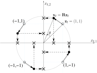
Figure 1: The system model of the toy example is illustrated. The coded bits are first mapped to a point in the constellation $\Omega_{\mathbf{z}}$ (empty circles), which is transformed to a point in the constellation $\Omega_{\mathbf{x}}$ (filled circles). The projections of the points of $\Omega_{\mathbf{x}}$ on the coordinate axes (marked by crosses) illustrates the component interleaving. The first and second component of $\mathbf{x}_{t}$, $x_{t,1}$ and $x_{t,2}$, $\forall t$, are affected by the fading gains $\beta_{1}$ and $\beta_{2}$, respectively.

According to Def. 1, bad precoders are rotation matrices $Q$ with rotation angle $\theta\in\theta_{\textrm{bad}}=\{k\pi/4,k=0,\ldots,7\}$, in which case some crosses in Fig. 1 coincide.

In the literature, only deterministic rotations were studied. Here, we study two other cases:

• $\theta$ is random, but fixed once it is chosen (Sec. IV-A);

• $\theta$ is random and independently generated at each channel use (Sec. IV-B).

The first case is similar to a non-ergodic MIMO channel, where the channel is random but remains constant during the transmission of an outer codeword. The second case is similar to a non-ergodic MIMO channel with a time-varying space-only precoder $P_{t}$ at its input.

IV-A Random rotation

It is well known [6, 23, 13] that a diversity order of two (denoted as full diversity in this section) is achieved for any coding rate $R_{c}\leq 1$ (including uncoded communication) when a fixed deterministic rotation matrix $Q$ is used and $s_{t,i}\neq 0,\forall~{}t,i,\forall~{}\mathbf{z}^{\prime}\neq\mathbf{z}$, where $\mathbf{s}_{t}=\mathbf{x}_{t}-\mathbf{x}_{t}^{\prime}$. In the context of MIMO, it is more interesting to consider a random rotation matrix $Q$. Despite the fact that $\textrm{Pr}(\theta\in\theta_{\textrm{bad}})=0$ when $p(\theta)=\frac{1}{2\pi}$, full diversity is not achieved as proved by the following lemma.

Lemma 1

In a point-to-point flat parallel Rayleigh fading channel as given in (14) with a fixed but random precoder $Q$ where $\theta$ follows a uniform distribution in $[0,2\pi]$, the diversity order can not be larger than $1.5$ for any coding rate $0.5<R_{c}<1$.

Proof:

See App. -B. ∎

From the proof of Lemma 1, it is clear that corrupt precoders (and not bad precoders) are the main cause of the full diversity loss. We formally define corrupt precoders in Sec. V, but for this section, consider corrupt precoders as the set of rotations where $\theta\in[0,\gamma^{-0.5}]$ . The probability to have such a corrupt precoder is proportional to $\gamma^{-0.5}$. When a precoder is corrupt, then the mutual information is strictly smaller than one in the event of one bad fading gain (see App. -B for a formal definition of bad fading). In this case, a coding rate larger than one-half leads to a spectral efficiency that is larger than one, yielding an outage event. The probability of a bad fading gain, which yields an outage event in conjunction with a corrupt precoder, is proportional to $\gamma^{-1}$. The probability of corrupt precoders is unfortunately non-negligible. Lemma 1 is corroborated by means of numerical simulations, presented in Fig. 2.

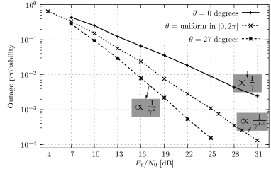
Figure 2: The outage probability of a parallel channel with two states does not achieve full diversity when the input constellation is rotated with a rotation angle that is random (uniform in $[0,2\pi]$) but fixed once it is chosen. For reference, the outage probabilities with a fixed rotation (with $\theta=0$ and $27$ degrees, corresponding to a bad and good rotation) are given. Other simulation parameters: $\Omega_{z}=$BPSK and $R_{c}=0.9$.

When the rotation angle is zero, we have a bad precoder and no transmit diversity is achieved. When the rotation angle is constant and different from $\{k\pi/4\}$, full transmit diversity is achieved. However, when the rotation angle is random, full transmit diversity is not achieved.

IV-B Random time-varying rotation

The effect of corrupt precoders can be easily reduced by using multiple random precoders, say $N$, during the transmission of one codeword. We leave a formal description for Sec. VII but qualitatively describe what happens in the case of the toy example. The probability to have one bad fading gain behaves as $\frac{1}{\gamma}$ (the probability of having two bad fading gains is not dominant, as it behaves as $\frac{1}{\gamma^{2}}$ and thus automatically leads to full diversity). Given that one fading gain is bad, the mutual information at high SNR converges to one and two for corrupt and non-corrupt precoders, respectively. The mutual information is averaged over these $N$ precoders. We have to consider at most one corrupt precoder as the probability to have a corrupt precoders behaves as $\gamma^{-0.5}$, so that two corrupt precoders in conjunction with a bad fading gain also automatically yield full diversity. In that case, the mutual information for large SNR, averaged over $N$ precoders, converges to $2\frac{N-1}{N}+\frac{1}{N}=2(1-\frac{1}{2N})$, so that any coding rate smaller than $1-\frac{1}{2N}$ yields full diversity.

A similar reasoning is valid for MIMO, which is formalized in the next sections.

V Bad and Corrupt precoders for MIMO

The definition of bad precoders was given in Def. 1. Bad precoders decrease the maximal mutual information that can be achieved. Listing the bad precoders is laborious and is fortunately not required for the theoretical analysis of fixed and time-varying space-only codes in the remainder of the paper. For completeness, we illustrate the bad precoders for $\Omega_{z}=4-$QAM and a $2\times 2$ MIMO channel in App. -C.

Bad precoders are defined to yield at least one component of $\mathbf{s}_{t}$ with a zero magnitude. The following lemma proves that at most $n_{T}-1$ components of $\mathbf{s}_{t}$ can have a zero magnitude.

Lemma 2

At most $n_{T}-1$ elements of $\mathbf{s}_{t}$ can have a magnitude equal to zero.

Proof:

If $n_{T}$ elements of $\mathbf{s}_{t}$ have a zero magnitude, then $\exists~{}\mathbf{z},\mathbf{z}^{\prime}\neq\mathbf{z}$, satisfying $\mathbf{x}_{t}=\mathbf{x}_{t}^{\prime}$, which is impossible, because $V_{t}$ is a bijection (see Lemma 5 in App. -A). ∎

As illustrated in the toy example in Sec. IV, the loss of transmit diversity for space-only codes is caused by corrupt precoders, which is an uncountable set of precoders that behave similarly as bad precoders, in the sense that a number of components of $\mathbf{s}_{t}$ have a vanishing magnitude with the SNR, instead of being zero for bad precoders. We distinguish between two sets of precoders, $\mathcal{S}_{c,1}$ and $\mathcal{S}_{c,2}$, which we both refer to as corrupt precoders. The first set is relevant in the case where ${n_{R}}\geq n_{T}$.

Definition 2

We define the set $\mathcal{S}_{c,1}$ of corrupt precoders as the set of precoders so that $\exists~{}\mathbf{z},\mathbf{z}^{\prime}\neq\mathbf{z}$, satisfying $|s_{t,i}|\leq\gamma^{-0.5},\forall~{}i>1$.

For the case that ${n_{R}}<n_{T}$, we define corrupt precoders as follows.

Definition 3

We define the set $\mathcal{S}_{c,2}$ of corrupt precoders as the set of precoders so that $\exists~{}\mathbf{z},\mathbf{z}^{\prime}\neq\mathbf{z}$, satisfying $|s_{t,i}|\leq\gamma^{-0.5},i=1,\ldots,{n_{R}}$.

Even without determining the structure of these precoders, we can derive their probability of occurrence.

Lemma 3

The probability that a random precoder falls in the set of corrupt precoders is

$$\textrm{Pr}(\mathcal{S}_{c,1})\dot{=}\gamma^{-(n_{T}-1)},~{}~{}~{}\textrm{Pr}(\mathcal{S}_{c,2})\dot{=}\gamma^{-{n_{R}}}.$$ (15)

for the sets $\mathcal{S}_{c,1}$ and $\mathcal{S}_{c,2}$, respectively.

Proof:

See App. -D. ∎

In the remainder of the paper, we use the notation $\mathcal{S}_{c}$, which refers to $\mathcal{S}_{c,1}$ or $\mathcal{S}_{c,2}$, when ${n_{R}}\geq n_{T}$ and ${n_{R}}<n_{T}$, respectively. As we will see in Sec. VI, the probability $\textrm{Pr}(\mathcal{S}_{c})$ is non-negligible and causes the loss of transmit diversity.

VI Fixed space-only codes

Consider a unitary but fixed space-only precoder $P_{t}=P$, hence $V_{t}$ is random (uniformly distributed in the set of all unitary matrices $\mathcal{M}(n_{T},n_{T})$ (Lemma 5)), but fixed once it is chosen. Because $V_{t}$ remains constant during the transmission of an outer codeword, we drop the index $t$ in the vectors $\mathbf{x}_{t},\mathbf{y}_{t}$ and $\mathbf{w}_{t}$, and denote $V^{\prime}=V^{\dagger}P$. A new channel $H^{\prime}=U\Sigma V^{\prime}$ is formed, which has the same distribution as $H$ because $V^{\prime}$ has the same distribution as $V^{\dagger}$. As a consequence, a fixed space-only precoder does not achieve transmit diversity.

In Sec. III, the relation between MIMO and parallel channels was given. More specifically, a MIMO channel is equivalent to a parallel channel with random precoding. The probability of having a bad precoder (Def. 1) is zero, but corrupt precoders cause the diversity loss, which is formalized in the following lemma.

Lemma 4

In a point-to-point flat fading $n_{T}\times{n_{R}}$ MIMO channel with a fixed $n_{T}\times n_{T}$ precoder $P_{t}=P$, there exists a coding rate $R_{c}<1$ above which the receive diversity is achieved (i.e., the outage SNR exponent is $d_{\textrm{out}}={n_{R}}$) due to corrupt precoders $V^{\prime}\in\mathcal{S}_{c}$.

Proof:

See App. -F. ∎

In accordance with the terminology of parallel channels with precoding, the loss of transmit diversity is caused because the random precoder falls too often in the set of corrupt precoders, or more precisely, because the probability to have a corrupt precoder does not converge fast enough to zero. Note that $\mathcal{S}_{c,1}$ contains precoders with constraints on $n_{T}-1$ components of $\mathbf{s}_{t}$. A larger set, having constraints on less than $n_{T}-1$ components can be defined as well, but leads to a less tight lower bound on the outage probability when using the same proof techniques as in App. -F.

Adopting a time-varying precoder $P_{t}$, uniform in the set of unitary matrices, within the coherence time of the channel (thus, assuming that the MIMO channel remains constant) has no effect on the diversity order for an uncoded scenario with respect to a fixed space-only code $P$. The reason is that the new channel $H^{\prime}=U\Sigma V_{t}$ still has the same distribution as $H$, with $V_{t}=V^{\dagger}P_{t}$.

VII Time-varying space-only codes, achieving full rate and full diversity

We propose to reduce the effect of corrupt precoders by averaging the mutual information over $N$ unitary precoders $V_{t}=V^{\dagger}P_{t}$ during the transmission of a codeword. We create $N$ realizations $V_{t}$ by changing $P_{t}$ after every $\frac{N_{c}}{N}$ channel uses. When $N$ is finite, the time-varying space-only code is denoted as EMI-$N$ code. In this section, we assume that $N=N_{c}$ and $N_{c}\rightarrow\infty$; the corresponding time-varying space-only code is denoted as EMI code. The convergence properties of the EMI-$N$ code are discussed in Sec. VIII-B. By letting $P_{t}$ being uniformly distributed in the set of all unitary matrices $\mathcal{M}(n_{T},n_{T})$, the matrix $V_{t}$ is also uniformly distributed in $\mathcal{M}(n_{T},n_{T})$ (Lemma 5). Furthermore, by drawing $P_{t}$ independently at each channel use, $V_{t}$ changes independently at each channel use.

Note that the bottom $n_{T}-{n_{R}}$ elements of $\mathbf{z}$ are zero when ${n_{R}}<n_{T}$, see Sec. II-B.

Theorem 1

In a point-to-point flat fading $n_{T}\times{n_{R}}$ MIMO channel, using a coding rate $R_{c}<1$ and using $n_{T}\times n_{T}$ precoders $P_{t}$, randomly generated for each channel use, being uniformly distributed in the set of all unitary matrices $\mathcal{M}(n_{T},n_{T})$, full diversity is achievable.

Proof:

See App. -G. ∎

Note that in (59) in App. -G, we used the fact that the temporal mean equals the sample mean, i.e.,

$$\mathbb{E}_{t}\left[I(\mathbf{x}_{t};\mathbf{y}_{t}|\Sigma,V_{t})\right]=\mathbb{E}\left[I(\mathbf{x}_{t};\mathbf{y}_{t}|\Sigma,V_{t})\right],$$ (16)

where the expectation at the right side in (16) is over $V_{t}$, uniformly distributed in the set of unitary matrices $\mathcal{M}(n_{T},n_{T})$, for a fixed $t$. This is valid for the EMI code.

Theorem 1 corroborates experimental results in the literature. For example, in [27, 32], the precoder $P_{t}$ was made variable by multiplying an initial precoder $P_{0}$ by a diagonal matrix $A_{t}$ including $e^{j2\pi\theta_{i}(t)}$ on the $i$-th diagonal element, where $\theta_{i}(t)$ varies each channel use. The overall precoder $P_{0}A_{t}$ is unitary and time-varying. Because the multiplication with $A_{t}$ corresponds to adding a time-varying phase to the complex baseband signal at each transmit antenna, the scheme was referred to as phase sweeping. Simulation results in [27, 32] suggest that full diversity is achieved in the presence of an error-correcting code with a particular coding rate. Theorem 1 now proves that full diversity is actually achievable (through the outage probability) for codes with any coding rate smaller than one, as long as $P_{t}$ is uniform in the set of unitary matrices.

VIII Numerical results

In this section, we corroborate Theorem 1 by numerically determining the outage probability for the EMI-$N$ code, which are also compared with the outage probabilities of approximately universal space-time codes. Despite being an unfair comparison taking into account the detection complexity, it allows to assess the loss of coding gain as a price for the reduced detection complexity associated with the EMI code. The outage probabilities are achievable lower bounds of the word error rate (WER) of practical coded systems. Therefore, it is useful to compare the outage probabilities with the WER of a coding scheme having the EMI code as inner code and an error-correcting code as outer code.

In Sec. VIII-A, we discuss the optimization of LDPC codes as outer code in such a coding scheme. Next, the convergence properties of the EMI-$N$ code to the EMI code are discussed in Sec. VIII-B. In the last two subsections, we present the numerical results for the $n_{T}\times{n_{R}}$ MIMO channel with ${n_{R}}\geq n_{T}$ and ${n_{R}}<n_{T}$, respectively.

The outage probabilities and WERs of the LDPC coded modulations are determined by means of Monte Carlo simulations. If the decoding complexity of exhaustive ML-detection of the STCs was too high, then sphere decoding is performed [46, 1, 7]. More specifically, soft output sphere decoding is performed [7], so that the Tanner graph of the LDPC code gets a soft input from the detectors of the STC. Iterative decoding and detection is performed, where after every 10 LDPC decoding iterations, a new detection of the STC is performed. The LDPC code is decoded by means of the sum-product algorithm on the Tanner graph. The total number of decoding iterations is limited by $100$.

The computation of (12) in the numerical calculation of the outage probability is in some cases (e.g. for approximately universal STCs, large constellation size or too many transmit antennas) time consuming because the constellation $\Omega_{\mathbf{x}}$ might be very large. Therefore, the inner sum over $\mathbf{x}_{t}^{\prime}\in\Omega_{\mathbf{x}}$ in (12) is simplified by using a sphere decoder. The sphere decoder outputs a list of maximum likelihood metrics $d^{2}(\mathbf{y}_{t},\sqrt{\gamma}\Sigma\mathbf{x}_{t}^{\prime})$ for all closest constellation points to the constellation point with the highest likelihood [1]. The list size is limited to $1000$.

VIII-A LDPC code optimization for the EMI code

We focus on binary LDPC codes $\mathcal{C}[N_{b},K_{b}]_{2}$ with dimension $K_{b}$, so that the coding rate $R_{c}=\frac{K_{b}}{N_{b}}$. Irregularity is introduced through the standard bit and check node degree distributions, characterized by the polynomials $\lambda(x)$ and $\rho(x)$, here from an edge perspective [39].

It is worth citing [43, 50, 51] and references therein, where the degree distributions of LDPC codes have been optimized for Gaussian and ergodic MIMO channels. However, optimizing these degree distributions for a non-ergodic MIMO channel (hence, where the random channel remains constant during the whole codeword) has not yet been performed to the best knowledge of the authors. In Sec. III, we have explained that the non-ergodic MIMO channel is equivalent to a parallel channel with a random precoder. To the authors’ best knowledge, only [12] presented a tool to optimize the degree distributions of an LDPC code for parallel Rayleigh faded channels with precoding. We therefore utilized the techniques from [12] to generate the degree distributions of the LDPC code.

We briefly describe the techniques developed in [12], where coded modulations (including the precoding matrix, the mapping function and the error-correcting code) were optimized to yield a WER closely approaching the outage probability. The off-line optimization, done using a geometric approach, was limited to at most $B+1$ times the effort for Gaussian channels, where $B$ is the number of parallel channels, here $\min(n_{T},{n_{R}})$. The geometric approach involves optimizing the coded modulation, e.g. via EXIT charts, in $B+1$ well chosen points in the $B$-dimensional fading plane. More specifically, in $B$ fading points on the $B$ axes of the fading plane close to the outage boundary, plus one fading point on the ergodic line ($\alpha_{1}=\ldots=\alpha_{B}$). The outage boundary limits the set of fading gain vectors for which the instantaneous mutual information is smaller than the spectral efficiency. More details on the outage boundary and the optimization of the outage probability through a proper selection of the precoding matrix and the constellation $\Omega_{\mathbf{z}}$ can be found in [13].

The main difference between the current channel equation (see Eq. 10) and the channel model in [12] is that the precoder $V_{t}$ is random. Hence, the instantaneous mutual information $I(\mathbf{x}_{t};\mathbf{y}_{t}|\Sigma,V_{t})$ does not only depend on the instantaneous realization of $\Sigma$, but also on the precoder realization $V_{t}$ (Fig. 3(b) shows the variation of the instantaneous mutual information with $V_{t}$). Because of the dependence on $V_{t}$, an outage boundary for the singular values $\{\sigma_{i},i=1,\ldots,\min({n_{R}},n_{T})\}$ cannot be defined based on $I(\mathbf{x}_{t};\mathbf{y}_{t}|\Sigma,V_{t})$. However, when the EMI-code is used, the mutual information is averaged over all unitary precoders in $\mathcal{M}(n_{T},n_{T})$, so that the mutual information $\mathbb{E}_{t}[I(\mathbf{x}_{t};\mathbf{y}_{t}|\Sigma,V_{t})]$ only depends $\Sigma$. We define the corresponding outage boundary as the set of singular values $\{\sigma_{i},i=1,\ldots,\min({n_{R}},n_{T})\}$ which yield $\mathbb{E}_{t}[I(\mathbf{x}_{t};\mathbf{y}_{t}|\Sigma,V_{t})]=R$. In practice, we approximate $\mathbb{E}_{t}[I(\mathbf{x}_{t};\mathbf{y}_{t}|\Sigma,V_{t})]$ by averaging $I(\mathbf{x}_{t};\mathbf{y}_{t}|\Sigma,V_{t})$ over a large number (e.g. $100$) of randomly generated matrices $V_{t}$. Fig. 3(a) illustrates such an outage boundary.

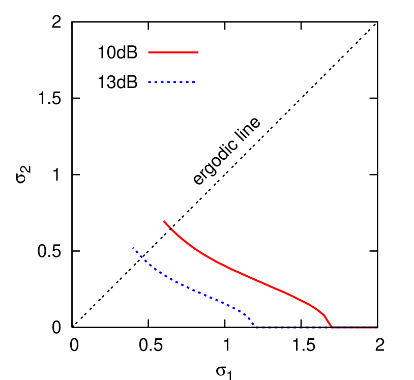
(a) The outage boundary is shown at two SNR values: $E_{b}/N_{0}=10$ dB and $E_{b}/N_{0}=13$ dB. Only half of the plane is used, as we consider the ordered singular values, $\sigma_{1}\geq\sigma_{2}$.

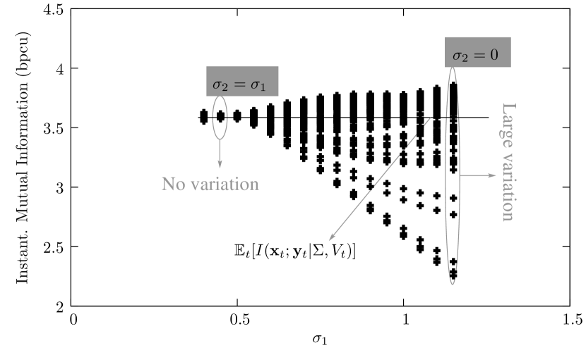
(b) The mutual information $I(\mathbf{x}_{t};\mathbf{y}_{t}|\Sigma,V_{t})$ largely varies with $V_{t}$ while $(\sigma_{1},\sigma_{2})$ is on the outage boundary, especially when $\sigma_{1}\gg\sigma_{2}$. For a given $\Sigma$, the values of $100$ mutual informations $I(\mathbf{x}_{t};\mathbf{y}_{t}|\Sigma,V_{t})$ are displayed, each corresponding to a realization of $V_{t}$. The adopted SNR is $E_{b}/N_{0}=13$ dB.

Figure 3: At the left side, the outage boundary is shown for $2\times 2$ MIMO with $\Omega_{z}=4$-QAM and $R=3.6$ bpcu, which is the set of singular values $(\sigma_{1},\sigma_{2})$ where $\mathbb{E}_{t}[I(\mathbf{x}_{t};\mathbf{y}_{t}|\Sigma,V_{t})]$ is equal to $R$. We approximated $\mathbb{E}_{t}[I(\mathbf{x}_{t};\mathbf{y}_{t}|\Sigma,V_{t})]$ by averaging $I(\mathbf{x}_{t};\mathbf{y}_{t}|\Sigma,V_{t})$ over $100$ randomly generated matrices $V_{t}$. The variation of $I(\mathbf{x}_{t};\mathbf{y}_{t}|\Sigma,V_{t})$ with $V_{t}$ is illustrated at the right side, where $(\sigma_{1},\sigma_{2})$ are located on the outage boundary (the outage boundary is a one-dimensional line, so that only one parameter, e.g. $\sigma_{1}$, is sufficient to characterize the location on this line).

As a consequence, the same method as in [12] can be applied to generate LDPC code degree distributions when using the EMI inner code.

VIII-B Maximal coding rate for the EMI-$N$ code

Theorem 1 proved that full diversity is achieved by the EMI code for any coding rate $R_{c}<1$. When $P_{t}$ changes a finite number of times $N$ during a codeword transmission, (16) and thus the proof in App. -G, are not valid. The maximum coding rate yielding full diversity may be smaller than for the EMI code. In this section, we provide an upper bound on the maximal coding rate yielding full diversity for the EMI-$N$ code, together with supporting numerical results.

As the probability of occurrence of corrupt precoders is strictly larger then $\gamma^{-nr}$, the occurrence of corrupt precoders amongst the $N$ precoders observed during the transmission of a codeword has to be considered. To derive the maximal coding rate yielding full-diversity, the maximal mutual information that can be achieved between input and output, when the input is transformed by a corrupt precoder, needs to be determined. Then, through a similar formula as Eq. (63), the maximal coding rate could be determined.

For example, consider the different classes of bad precoders for the $2\times 2$ MIMO channel and $\Omega_{z}=4$-QAM, which are given in Eq. (38). Each type of bad precoder corresponds to a maximum achievable mutual information $I(\mathbf{x}_{t};\mathbf{y}_{t}|\Sigma,V_{t})$, which for the precoders from (38) are given by $\{2,2,\log_{2}9,\log_{2}12,\log_{2}12\}$. This can be verified analytically or by means of simulation. Next, different subsets of the set of corrupt precoders will have a maximal mutual information that converges to the maximal mutual information of one of the bad precoders for increasing SNR. Each subset will have to be defined more precisely than in Defs. 2 and 3, i.e., some subsets will have more than one pair of $\mathbf{z},\mathbf{z}^{\prime}$ yielding $|s_{t,i}|\leq\gamma^{-0.5}$ for some $i$. Therefore, some subsets might have a smaller probability of occurrence than what is given in Lemma 3.

A detailed study of this behaviour is outside the scope of this work. However, we can provide an upper bound on the maximal coding rate yielding full diversity, by assuming an optimistic case. Instead of averaging $I(\mathbf{x}_{t};\mathbf{y}_{t}|\Sigma,V_{t})$ over $V_{t}=V^{\dagger}P_{t}$ by changing $P_{t}$, we can consider the average of $I(\mathbf{x}_{t};\mathbf{y}_{t}|H)$ over $N$ realizations of $H$, corresponding to a block fading MIMO channel with $N$ states. The achievable diversity order for a block fading MIMO channel with $N$ blocks is upper bounded by [26]

$$d_{\textrm{up}}={n_{R}}(\lfloor Nn_{T}(1-R_{c})\rfloor+1).$$ (17)

Hence, by putting $d_{\textrm{up}}\geq nr$, we get after some calculus that

$$R_{c,\textrm{max}}\leq 1-\frac{1}{N}+\frac{1}{nN}.$$ (18)

Further work must verify whether this bound is tight for the EMI-$N$ code.

The theoretical analysis is laborious, but conjectures can be made from the numerical simulations by comparing the diversity order of the EMI-$N$ code with that of the EMI code, which achieves full diversity (Fig. 4). When using $N=2$, it may be conjectured that the bound in Eq. (18) is achieved as full diversity is still achieved for a coding rate $R_{c}=0.75$. When using $N=10$, full diversity is still achieved for a coding rate $R_{c}=0.9$. However, at a coding rate $R_{c}=0.95$, which corresponds to the bound in Eq. (18), full diversity is not achieved.

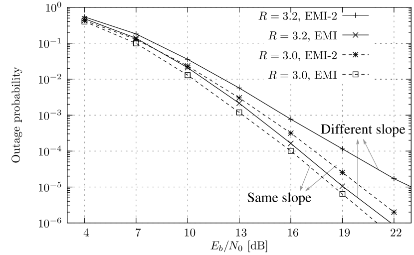
(a) The outage probabilities of the EMI-$2$ for $R=\{3,~{}3.2\}$ bpcu are shown. It may be conjectured that full diversity is achieved for rates not larger than $R=3.0$ bpcu, which corresponds to $R_{c}=0.75$.

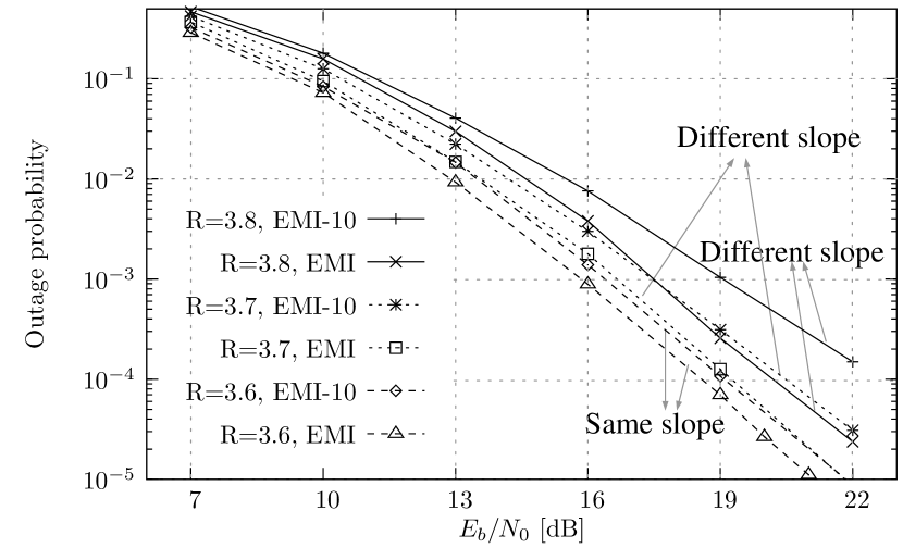
(b) The outage probabilities of the EMI-$10$ for $R=\{3.6,~{}3.7,~{}3.8\}$ bpcu are shown. It may be conjectured that full diversity is achieved for rates $R\leq 3.6$ bpcu, which corresponds to $R_{c}=0.9$.

Figure 4: It can be numerically verified whether the EMI-$N$ code (EMI-$2$ at the left side and EMI-$10$ at the right side) achieves full diversity by comparing its outage probability to that of the EMI-code, which always achieves full diversity. Simulation parameters: $2\times 2$ MIMO with $\Omega_{z}=4$-QAM and different rates.

Because it is difficult to design very high coding rate error-correcting codes (see [48] and references therein), coding rates larger than $R_{c}=0.9$ almost never occur in practice. Therefore, we only consider the EMI-$10$ code, achieving full diversity at coding rates smaller than or equal to $R_{c}=0.9$, in the remainder of the paper, unless mentioned otherwise.

VIII-C Numerical results for the $n_{T}\times{n_{R}}$ MIMO, ${n_{R}}\geq n_{T}$

When ${n_{R}}\geq n_{T}$, a transformation of $n_{T}$ independent symbols are transmitted at each channel use. We compare the outage and error rate performance of the EMI-$10$ code with STCs from the literature that are optimal in terms of uncoded error rate (e.g., [4, 21] and [8]) or optimal in terms of error rate assuming a genie condition (e.g., [8] and [26]). We also include the error rate performance without precoding (which is equivalent to a fixed space-only code) for reference.

First, let us consider the $2\times 2$ MIMO channel and $\Omega_{z}=4$-QAM. Fig. 5 compares the performances of the Golden code [4] with the EMI-$10$ code and the case without precoding. The performance of other STCs, such as [8, 26] were also tested, but their error rates are slightly larger than that of the Golden code, so that they are not displayed for clarity. The LDPC code of $R_{c}=0.9$ is a regular $(3,30)$ LDPC code, which showed the best performance among other tested LDPC codes of the same coding rate. The code length of the LDPC code is $N_{b}=5760$.

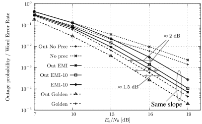
Figure 5: For a coding rate $R_{c}=0.9$ (i.e., $R=3.6$ bpcu) and a $2\times 2$ MIMO channel, the outage probabilities of the EMI and EMI-$10$ code achieve full diversity and perform at $1.5$ and $2$ dB from the outage probability of the Golden code. “Out” stands for outage probability, the other curves represent the WER of a practical system with an error-correcting code.

As theoretically proved in Theorem 1, full diversity is achieved by the EMI code. The focus of this paper was on full rate, full diversity, and low decoding complexity. Of course, the significant reduction in complexity comes at the expense of a loss in coding gain (the EMI and EMI-$10$ code respectively require $1.5$ and $2$ dB more energy to have the same error rate performance than the Golden code). However, as shown in Figs. 6 and 7, this loss in coding gain vanishes when the coding rate decreases. More spefically, the loss in coding gain is around $0.5$ dB when $R_{c}=0.75$ and $0$ dB when $R_{c}=0.55$. In Figs. 6 and 7, the outage probability of the EMI and EMI-$10$ code coincide, so that the EMI code is not shown for clarity. Similarly, the error rates of the Golden code and the STCs from [8, 26] practically coincide. The degree distributions of the LDPC code were obtained as explained in Sec. VIII-A and are given by

$$\lambda(x)=0.231x+0.543x^{2}+0.226x^{19};~{}~{}~{}\rho(x)=x^{12}$$

for $R_{c}=0.75$ and by

$$\lambda(x)=0.215x+0.465x^{2}+0.040x^{19}+0.280x^{20};~{}~{}~{}\rho(x)=x^{7}$$

for $R_{c}=0.55$. The code length is $N_{b}=5760$.

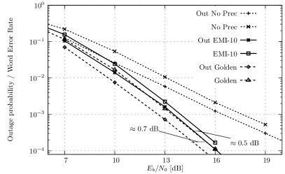
Figure 6: For a coding rate $R_{c}=0.75$ (i.e., $R=3.0$ bpcu), the horizontal SNR-gap between the outage probabilities of the EMI-$10$ code and the Golden code reduced from $2$ dB (for $R_{c}=0.9$) to $0.5$ dB. Other simulation parameters: $2\times 2$ MIMO, “Out” stands for outage probability, the other curves represent the LDPC code WER.

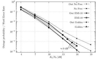
Figure 7: For a coding rate $R_{c}=0.55$ (i.e., $R=2.2$ bpcu), the horizontal SNR-gap between the outage probabilities of the EMI-$10$ code and the Golden code has vanished. Other simulation parameters: $2\times 2$ MIMO, “Out” stands for outage probability, the other curves represent the LDPC code WER.

Next, we consider the $2\times 3$ and $3\times 3$ MIMO channels using $\Omega_{z}=4$-QAM. Figs. 8 and 9 compare the performances of approximately universal STCs (the Golden code [4] for $n_{T}=2$ and the Perfect STC [21] for $n_{T}=3$) with the EMI-$10$ code and the case without precoding. Other STCs, such as [8, 26] for $n_{T}=2$, have a similar or slightly degraded error rate performance, so that they are not displayed for clarity. The LDPC code of $R_{c}=0.9$ is again a regular $(3,30)$ LDPC code and the code length of the LDPC code is $N_{b}=5760$.

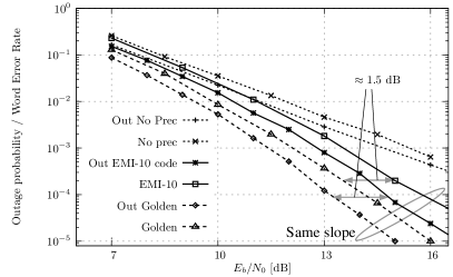
Figure 8: The EMI-$10$ code also achieves full diversity for $R_{c}=0.9$ (i.e., $R=3.6$ bpcu) and the $2\times 3$ MIMO channel, performing at approximately $1.5$ dB from the Golden code. “Out” stands for outage probability, the other curves represent the LDPC code WER.

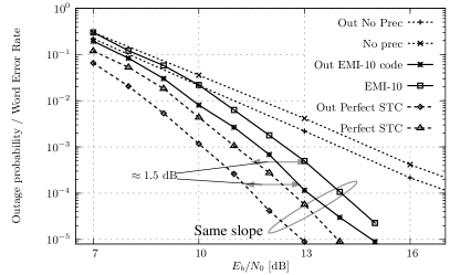
Figure 9: Also for the $3\times 3$ MIMO channel and $R_{c}=0.9$ (i.e., $R=5.4$ bpcu), full-diversity is achieved by the EMI-$10$ code, again performing at approximately $1.5$ dB from the approximately universal code, denoted as perfect STC. “Out” stands for outage probability, the other curves represent the LDPC code WER.

Full diversity is achieved by the EMI-$10$ code and as for the $2\times 2$ MIMO channel, the significant reduction in complexity comes at the expense of a loss in coding gain when the coding rate is close to one. When $R_{c}=0.9$, this loss is approximately $1.5$ dB.

Finally, we consider a larger constellation size for the $2\times 2$ MIMO channel, using $\Omega_{z}=16$-QAM (Fig. 10). The other parameters, such as the degree distributions, coding rate and the code length are the same. The performance of the EMI-$10$ code is compared with those of the Golden code, the cyclotomic code [26] and Aladdin-Pythagoras code [8]. The loss in coding gain of the EMI-code is not larger than $1.5$ dB.

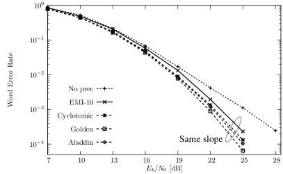
Figure 10: Also for higher constellation sizes (here $\Omega_{z}=16$-QAM), the EMI-$10$ code achieves full diversity in terms of WER. Other simulation parameters: $2\times 2$ MIMO, $R_{c}=0.9$ ($R=7.2$ bpcu).

VIII-D Numerical results for the $n_{T}\times{n_{R}}$ MIMO, ${n_{R}}<n_{T}$

When ${n_{R}}<n_{T}$, a transformation of, on average, ${n_{R}}$ independent symbols are transmitted at each channel use. For the $2\times 1$ MIMO channel, the Alamouti code [2] is well known to be optimal in many ways, e.g. in terms of uncoded error rate. The loss of coding gain of the EMI-$N$ code is quite large (e.g., more than $3$ dB for $R_{c}=0.9$) when the coding rate is close to one, but decreases with the coding rate (e.g., around $1.5$ dB for $R_{c}=0.75$), see Fig. 11.

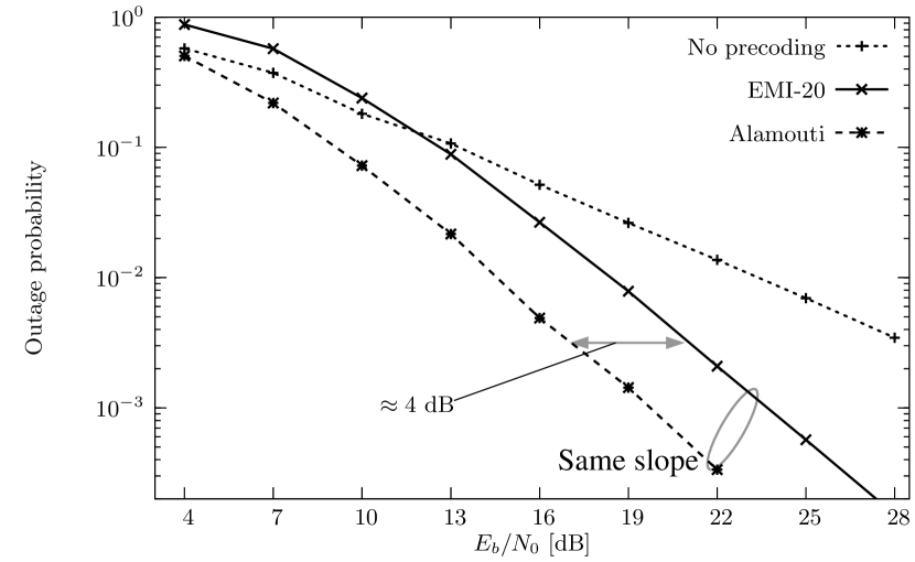
(a) For $R_{c}=0.9$ (i.e., $R=1.8$ bpcu), the outage probability of the EMI-$20$ code performs at approximately $4$ dB from the Alamouti code.

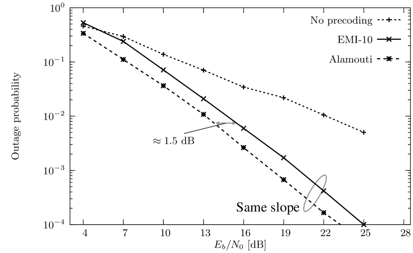
(b) The horizontal SNR-gap with the Alamouti code reduced to approximately $1.5$ dB for $R=1.5$ bpcu ($R_{c}=0.75$).

Figure 11: The outage probability of the EMI-$N$ code is compared with the Alamouti STC for the $2\times 1$ MIMO channel with $\Omega_{z}=4$-QAM and rates $1.8$ bpcu (left) and $1.5$ bpcu (right). Full diversity is achieved but the loss of coding gain is large.

It may be conjectured that the EMI-$N$ code can not compete with the Alamouti code for the $2\times 1$ MIMO channel, given that the Alamouti code also has a low detection complexity.

For completeness, we also show the outage probability of the EMI-$N$ code for the $3\times 1$ MIMO channel (Fig. 12), which corroborates Theorem 1, i.e., full diversity is achieved, also when ${n_{R}}<n_{T}$.

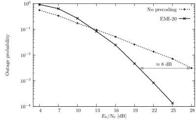
Figure 12: We show that the outage probability of the EMI-$20$ code achieves full diversity on the $3\times 1$ MIMO channel for $\Omega_{z}=4$-QAM and $R_{c}=0.9$ (i.e., $R=1.8$ bpcu).

IX Conclusion

For unknown channel state information at the transmitter, we proposed a new coded modulation paradigm: outer error-correction code with space-only but time-varying precoding. Full diversity is proved in terms of the outage probability and verified by means of numerical simulations. The proofs are based on the relation between MIMO and parallel channels. For most coding rates, using ten space-only precoders per codeword is sufficient and the error rate performance of LDPC coded modulations approaches the outage probability. The detection complexity of space-only codes is significantly smaller than for approximately universal space-time codes, coming at a price of coding gain loss for coding rates $R_{c}$ close to one (e.g. $1.5$ dB for $R_{c}=0.9$), which fortunately vanishes with decreasing coding rate.

References

- [1] E. Agrell, T. Eriksson, A. Vardy, and K. Zeger, “Closest point search in lattices,” IEEE Trans. on Inf. Theory, vol. 48, no. 8, pp. 2201-2214, Aug. 2002.
- [2] S.M. Alamouti, “A simple transmit diversity technique for wireless communications,” IEEE J. on Sel. Ar. in Comm., vol. 16, no. 8, pp. 1451-1458, Oct. 1998.
- [3] D. Bayer-Fluckiger, F. Oggier, and E. Viterbo, “New algebraic constructions of rotated -lattice constellations for the Rayleigh fading channel,” IEEE Trans. on Inf. Theory, vol. 50, no. 4, pp. 702-714, Apr. 2004.
- [4] J.-C. Belfiore, G. Rekaya, and E. Viterbo, “The golden code: a 2x2 full rate space-time code with non-vanishing determinants,” IEEE Trans. on Inf. Theory, vol. 51, no. 4, pp. 1432-1436, Apr. 2005.
- [5] E. Biglieri, J. Proakis, and S. Shamai, “Fading channels: information-theoretic and communications aspects,” IEEE Trans. on Inf. Theory, vol. 44, no. 6, pp. 2619-2692, Oct. 1998.
- [6] J.J. Boutros and E. Viterbo, “Signal space diversity: a power- and bandwidth-efficient diversity technique for the Rayleigh fading channel,” IEEE Trans. on Inf. Theory, vol. 44, no. 4, pp. 1453-1467, July 1998.
- [7] J.J Boutros, N. Gresset, L. Brunel, and M. Fossorier, “Soft-input soft-output lattice sphere decoder for linear channels,” in Proc. IEEE Globecom Telecomm. Conf., vol. 3, pp. 1583-1587, Dec. 2003.
- [8] J.J. Boutros and H. Randriambololona, “The Aladdin-Pythagoras space-time code,” in Proc. IEEE Intern. Symp. on Inf. Theory (ISIT), pp. 2823-2827, July 2009.
- [9] Y. Choquet-Bruhat and C. Dewitt-Morette, Analysis, Manifolds and Physics, North-Holland, 1982.
- [10] T.M. Cover and J.A. Thomas, Elements of Information Theory, New York, Wiley, 1991.
- [11] R. Durrett, Probability: theory and examples, Cambridge University Press, 2010.
- [12] D. Duyck, J.J. Boutros, and M. Moeneclaey, “Precoding for Word Error Rate Minimization of LDPC Coded Modulations on Block Fading Channels,” submitted to IEEE Trans. on Wireless Comm., May 2011.
-
[13]
D. Duyck, J.J. Boutros, and M. Moeneclaey,
“Precoding for Outage Probability Minimization on Block Fading Channels,”
submitted to IEEE Trans. on Inf. Theory, March 2011, Download from. telin.ugent.be/
~dduyck/publications/Subm_IT_DD.pdf. - [14] D. Duyck, S. Yang, F. Takawira, J.J. Boutros, and M. Moeneclaey, “Time-Varying Space-Only Code: A New Paradigm for Coded MIMO Communication” in Proc. Int. Symp. on Comm., Contr. and Sign. Proc. (ISCCSP), Rome, Italy, May 2012.
- [15] D. Duyck, S. Yang, F. Takawira, J.J. Boutros, and M. Moeneclaey, “Time-Varying Space-Only Codes,” in Proc. IEEE Intern. Symp. on Inf. Theory (ISIT), July 2012.
- [16] A. Edelman and N.R. Rao, Random Matrix Theory, Cambridge University Press, 2005.
- [17] A. Edelman, Eigenvalues and Condition Numbers of Random Matrices, Ph.D. thesis, MIT, May 1989.
- [18] H. El Gamal, G. Caire, and M.O. Damen, “Lattice Coding and Decoding Achieve the Optimal Diversity-Multiplexing Tradeoff of MIMO Channels,” IEEE Trans. on Inf. Theory, vol. 50, no. 6, pp. 968-985, June 2004.
- [19] F. Oggier, G. Rekaya, J.-C. Belfiore, and E. Viterbo, “Perfect space-time block codes,” IEEE Trans. on Inf. Theory, vol. 52, no. 9, pp. 3885-3902, Sept. 2006.
- [20] P. Elia, K.R. Kumar, S.A. Pawar, P.V. Kumar, and H.-F. Lu, “Explicit, minimum-delay space-time codes achieving the diversity-multiplexing gain tradeoff,” IEEE Trans. on Inf. Theory, vol. 52, no. 9, pp. 3869-3884, Sep. 2006.
- [21] P. Elia, B.A. Sethuraman, and P.V. Kumar, “Perfect Space Time Codes for Any Number of Antennas,” IEEE Trans. on Inf. Theory, vol. 53, no. 11, pp. 3853-3868, Nov. 2007.
- [22] A. Guillén i Fàbregas and G. Caire, “Coded modulation in the block-fading channel: coding theorems and code construction,” IEEE Trans. on Inf. Theory, vol. 52, no. 1, pp. 91-114, Jan. 2006.
- [23] A. Guillén i Fàbregas and G. Caire, “Multidimensional coded modulation in block-fading channels,” IEEE Trans. on Inf. Theory, vol. 54, no. 5, pp. 2367-2372, May 2008.
- [24] G.J. Foschini, “Layered space-time architecture for wireless communication in fading environments when using multi-element antennas,” Bell Labs Tech. J., vol. 1, no. 2, pp. 41 59, Autumn 1996.
- [25] G.J. Foschini and M.J. Gans, “On Limits of Wireless Communications in a Fading Environment when Using Multiple Antennas,” Wireless Personal Communications, vol. 6, no. 3, pp. 311-355, Mar 1998.
- [26] N. Gresset, L. Brunel, and J.J. Boutros, “Space-time coding techniques with bit-interleaved coded modulations for MIMO block-fading channels,” IEEE Trans. on Inf. Theory, vol. 54, no. 5, pp. 2156-2178, May 2008.
- [27] A. Hiroike, F. Adachi, and N. Nakajima, “Combined effects of phase sweeping transmitter diversity and channel coding,” IEEE Trans. on Veh. Techn., vol. 41, no. 2, pp. 170-176, May 1992.
- [28] J. Jalden and P. Elia, “Sphere decoding complexity exponent for decoding full rate codes over the quasi-static MIMO channel,” submitted to IEEE Trans. on Inf. Theory, available Arxiv preprint:1102.1265, Feb. 2011.
- [29] N.L. Johnson, S. Kotz, and N. Balakrishnan, “Continuous univariate distributions,” Wiley, 1995.
- [30] E.R. Larsson and P. Stoica, Space-Time Block Coding for Wireless Communications, Cambridge University Press, 2003.
- [31] D.J. Love and R.W. Heath, “Limited feedback unitary precoding for spatial multiplexing systems,” IEEE Trans. on Inf. Theory, vol. 51, no. 8, pp. 2967-2976, Aug. 2005.
- [32] X. Ma and G.B. Giannakis, “Space-Time-Multipath Coding Using Digital Phase Sweeping or Circular Delay Diversity,” IEEE Trans. on Sign. Proc., vol. 53, no. 3, pp. 1121-1131, March 2005.
- [33] R. J. Muirhead, Aspects of Multivariate Statistical Theory. New York, Wiley, 1982.
- [34] L.P. Natarajan, P.K. Srinath, and B.S. Rajan, “Generalized Distributive Law for ML Decoding of STBCs,” in Proc. Inf. Theory Worksh. (ITW), Paraty, Brasil, Oct. 2011.
- [35] K.D. Nguyen, A. Guillén i Fàbregas, and L.K. Rasmussen, “A Tight Lower Bound to the Outage Probability of Discrete-Input Block-Fading Channels,” IEEE Trans. on Inf. Theory, vol. 53, no. 11, pp. 4314-4322, Nov. 2007.
- [36] C. Oestges and B. Clerckx, MIMO Wireless Communications: from real world propagation to space-time code design, Academic Press, Elsevier, 2007.
- [37] L.H. Ozarow, S. Shamai, and A.D. Wyner, “Information theoretic considerations for cellular mobile radio,” IEEE Trans. on Vehicular Technology, vol. 43, no. 2, pp. 359-379, May 1994.
- [38] K.P. Srinath and B.S. Rajan, “Low ML-Decoding Complexity, Large Coding Gain, Full-Rate, Full-Diversity STBCs for and MIMO Systems,” IEEE J. of Sel. Topics in Sign. Proc., vol. 3, no. 6, pp. 916–927, Dec. 2009.
- [39] T.J. Richardson, M.A. Shokrollahi, and R.L. Urbanke, “Design of capacity-approaching irregular low-density parity-check codes,” IEEE Trans. on Inf. Theory, vol. 47, no. 2, pp. 619-637, Feb. 2001.
- [40] V. Tarokh, N. Seshadri, and A.R. Calderbank, “Space-time codes for high data rate wireless communication: performance criterion and code construction,” IEEE Trans. on Inf. Theory, vol. 44, no. 2, pp. 744-765, Mar. 1998.
- [41] S. Tavildar and P. Viswanath, “Approximately Universal codes over slow fading channels,” IEEE Trans. on Inf. Theory, vol. 52, no. 7, pp. 3233-3258, Jul 2006.
- [42] I.E. Telatar, “Capacity of multi-antenna Gaussian channels,” Europ. Trans. on Telecomm., vol. 10, pp. 585-595, Nov./Dec. 1999.
- [43] S. ten Brink, G. Kramer, and A. Ashikhmin, “Design of Low-Density Parity-Check Codes for Modulation and Detection,” IEEE Trans. on Comm., vol. 52, no. 4, pp. 670–678, Apr. 2004.
- [44] D.N.C. Tse and P. Viswanath, Fundamentals of Wireless Communication, Cambridge University Press, May 2005.
- [45] G. Ungerboeck, “Channel coding with multilevel/phase signals,” IEEE Trans. on Inf. Theory, vol. IT-28, no. 1, pp. 55-67, Jan. 1982.
- [46] E. Viterbo and J.J. Boutros, “A Universal Lattice Code Decoder for Fading Channels,” IEEE Trans. on Inf. Theory, vol. 45, no. 5, pp. 1639-1642, July 1999.
- [47] J. Winters, “On the capacity of radio communication systems with diversity in a Rayleigh fading environment,” IEEE J. on Sel. Ar. in Comm., vol. 5, pp. 871 878, June 1987.
- [48] M. Yang, W.E. Ryan, and Y. Li, “Design of Efficiently Encodable Moderate-Length High-Rate Irregular LDPC Codes,” IEEE Trans. on Comm., vol. 52, no. 4, pp. 564-571, April 2004.
- [49] S. Yang and J.-C. Belfiore, “Distributed rotation recovers spatial diversity,” IEEE Intern. Symp. on Inf. Theory (ISIT), pp. 2158-2162 , June 2010.
- [50] G. yue and X. Wang, “Optimization of irregular repeat accumulate codes for MIMO systems with iterative receivers,” IEEE Trans. on Wir. Comm., vol. 4, no. 6, pp. 2843-2855, Nov. 2005.
- [51] J. Zheng and B.D. Rao, “LDPC-coded MIMO systems with unknown block fading channels: soft MIMO detector design, channel estimation, and code optimization,” IEEE Trans. on Sign. Proc., vol. 54, no. 4, pp. 1504-1518, Apr. 2006.
- [52] L. Zheng and D.N.C. Tse, “Diversity and Multiplexing: A Fundamental Tradeoff in Multiple-Antenna Channels,” IEEE Trans. on Inf. Theory, vol. 49, no. 5, pp. 1073-1096, May 2003.