Multiphoton transitions in Josephson-junction qubits
(Review Article)

Abstract

Two basic physical models, a two-level system and a harmonic oscillator, are realized on the mesoscopic scale as coupled qubit and resonator. The realistic system includes moreover the electronics for controlling the distance between the qubit energy levels and their populations and to read out the resonator’s state, as well as the unavoidable dissipative environment. Such rich system is interesting both for the study of fundamental quantum phenomena on the mesoscopic scale and as a promising system for future electronic devices.

We present recent results for the driven superconducting qubit - resonator system, where the resonator can be realized as an $LC$ circuit or a nanomechanical resonator. Most of the results can be described by the semiclassical theory, where a qubit is treated as a quantum two-level system coupled to the classical driving field and the classical resonator. Application of this theory allows to describe many phenomena for the single and two coupled superconducting qubits, among which are the following: the equilibrium-state and weak-driving spectroscopy, Sisyphus damping and amplification, Landau-Zener-Stückelberg interferometry, the multiphoton transitions of both direct and ladder-type character, and creation of the inverse population for lasing.

I 1. Introduction

A quantum system, subjected to external driving, can experience resonant transitions between its energy levels. Conservation of total energy assumes absorption or emission of several photons of the driving field. Such multiphoton processes play an important role in atomic and molecular systems interacting with electromagnetic field Coh-Tan . For example, the multiphoton resonant spectroscopy is one of the methods to probe the structure of atoms and molecules Delone . This technique has the advantage of observing highly excited states by using relatively low frequencies. The concept of another application, the multiphoton excitation microscopy, is based on the multiphoton excitation of the fluorescent dyes molecules Xu96 ; Konig00 ; Diaspro06 . This technique allows imaging biochemical objects with high spatial resolution.

Recent development of fabrication and measurement techniques enabled a study of the wide spectrum of quantum phenomena in superconducting structures. During the past years it has been clearly shown that specially designed macroscopic superconducting circuits, which include Josephson junctions, behave quantum mechanically similar to a quantum particle in a potential well. Under certain conditions, these objects demonstrate the coherent superposition between their macroscopically distinct quantum states. It is important to note that this is a pure quantum effect which has no classical analogue and can be used for a number of intrigued applications. If the circuit’s dynamics can be described in the frame of the two-level approximation, such two-level quantum system is called a qubit. The advance in the study of different phenomena in superconducting qubits can be found in the reviews Makhlin01 ; Devoret04 ; Wendin07 ; Clarke08 ; You11 .

In general, superconducting Josephson circuits can be described as multilevel quantum systems. By analogy, such systems are called artificial atoms, while coupled qubits systems behave as artificial molecules. An interesting problem is how phenomena, known from atomic physics, will appear for these artificial atoms and molecules. Note that the following features differ these mesoscopic-size quantum systems from their microscopic counterparts: a high level of controllability by electronic means, coupling to the macroscopic-size read-out devices, and unavoidable dissipative environment.

For characterization and controlling the states of superconducting qubits the one-photon spectroscopy was done by using relatively weak driving Nakamura99 ; Friedman00 ; vanderWal00 ; Vion02 ; Yu02 ; Martinis02 ; Chiorescu03 ; Born04 . Matching of the ground and higher states with the one-photon energy was exploited to probe the upper levels of the Josephson-junction circuits Claudon04 ; Berns08 ; Neely09 ; Nori09 ; Jirari09 ; Sillanpaa09 ; Joo10 ; Du10a . With increasing driving power, the multiphoton excitations were used to study the features of the artificial atoms both for the two-level dynamics Nakamura01 ; Wallraff03 ; Saito04 ; Shnyrkov06 ; Shnyrkov09  and when the upper levels were involved Yu05 ; Strauch07 ; Dutta08 ; Wang10 ; Bushev10 . For strong driving, the width of the resonance lines periodically tends to zero, which can be described as the destructive Landau-Zener-Stückelberg interference Shevchenko10 . Respective interferograms displayed double-periodical dependence of the upper-level occupation probability on the energy bias and the driving amplitude Oliver05 ; Sillanpaa06 ; Wilson07 ; Izmalkov08 ; Sun09 ; LaHaye09 .

Two and more coupled qubits can be treated as artificial molecules. Being excited by a resonant microwave field, they display one-photon transitions Pashkin03 ; Berkley03 ; Majer05 ; Steffen06 ; Plantenberg07 ; Fay08 ; DiCarlo09 ; Altomare10 . Alternatively, at smaller frequencies, the two-qubit systems can experience multiphoton transitions Leek09 ; Ilichev10 ; Temchenko11 ; Satanin12 .

In this article we review the observations of the multiphoton transitions in single and coupled superconducting qubits probed by a classical resonator, and also we present the respective theory. Having the purpose of presenting and describing specific results for the multiphoton transitions, our consideration is limited to the Josephson-junction qubits. We note however that similar phenomena can be studied in different quantum objects, which can be described as two- or multi-level systems, such as quantum wires and dots Ho09 ; Ribeiro10 ; Brataas11 ; Dovzhenko11 ; Gaudreau12 , nitrogen vacancy centers in diamond Childress10 ; Huang11 , ultracold atoms Zenesini10 ; Plotz10 ; Zhang11 , nanomechanical and optomechanical setups Heinrich10 ; Chotorlishvili11 ; Miladinovic11 , electronic spin systems, two-dimensional electron gas, and graphene Bertaina11 ; Hatke11 ; Avetissian11 .

The paper is organized as follows. In Sec. 2 we use the method of an asymptotic expansion for the qubit-resonator system in order to obtain the resonator characteristics. This formalism allows us to separate the dynamics of the relatively slow resonator and fast qubit. Then, in Sec. 3, we consider the multiphoton dynamics of an isolated two-level system. Later the formulas of those two sections will be applied for the description of the experimentally observed multiphoton excitations in single qubits (Sec. 4) and in coupled qubits systems (Sec. 5).

II 2. Semiclassical theory of the qubit-resonator system

For characterization of a quantum system different techniques can be applied. One of the possible solutions is to use the so-called parametric transducer Braginsky92 . A key element in any parametric transducer is an optical or a radio-frequency auto-oscillator. A transducer, coupled to the quantum system of interest, is constructed so, that quantum system dynamics causes a change of the phase or/and the amplitude of its oscillations. A phase (amplitude) shift provides information about the dynamics of a quantum system. In particular, for probing the qubit’s state, several types of oscillators have been already used: an $LC$ tank circuit Ilichev02 ; Ilichev09 , a nanomechanical one Irish03 ; LaHaye09 , and a transmission line resonator Blais04 ; Schuster05 . If the resonator quantization energy $\hbar\omega_{\mathrm{p}}$ is smaller than the thermal excitation energy $k_{\mathrm{B}}T$, the resonator can be considered as a classical oscillator. Then the qubit-resonator system can be treated semiclassically: here a qubits quantum system is driven by a classical field and probed by a classical oscillator. It is important to note that the similar approach is well known in quantum optics - many phenomena in the atom-light system can be described by making use of this semiclassical model Delone .

In this work we present the semiclassical description of some observed effects for the resonator-qubits systems. We will not consider here the situation of coupling the qubits systems to a high-frequency resonator, which can be realized as a transmission line resonator. The quantum properties of this qubit-resonator system are not described by the semiclassical model. For recent works in this field see e.g. Abdumalikov08 ; Oelsner09 ; Omelyanchouk10 ; Ashhab10 ; Niemczyk10 and references therein and also Refs. Bishop08 ; Niemczyk09 ; Fink09 , where the multiphoton excitations were used to drive transitions between the multiple energy levels of the qubit-resonator system in the strong coupling regime.

Another note here should be made about the term “multiphoton processes”. In the context of the semiclassical approach, it relates to the energy of several photons which is absorbed or emitted by the quantum system. In the broader sense the term “multiphoton” can relate to other processes employing the quantum nature of the electromagnetic field, see Ref. Pan11 for a review of the non-classical phenomena in entangled multi-photon systems.

This section is devoted to the properties of the qubit-resonator system. It will be shown that in the frame of the semiclassical approach the influence of the qubit on the resonator can be described by the “renormalization” of the oscillator constants. For instance for a mechanical resonator it can be quantified by introducing the equivalent qubit’s-state-dependent elasticity coefficient and damping factor. In the case of inductive/capacitive coupling, the qubit’s impact on the resonator can be described by introducing the qubit’s-state-dependent effective inductance/capacitance, while the losses can be described by the effective resistance. For concreteness, we will consider two realistic systems: the flux qubit inductively coupled to the tank circuit ShevchenkoPG08 and the charge qubit capacitively coupled to the nanomechanical resonator Shevchenko11 .

II.1 Krylov-Bogolyubov formalism for qubit-resonator system

First let us consider the mechanical resonator as a spring with the elasticity $k_{0}$, the damping factor $\lambda_{0}$ (which is assumed to be small), and loaded with mass $m$, as shown in Fig. 1(a). The oscillator has eigenfrequency $\omega_{0}=\sqrt{k_{0}/m}$ and the quality factor $Q_{0}=m\omega_{0}/\lambda_{0}$. Its state is influenced by the qubit through the force $\epsilon F_{\mathrm{q}}$ and is driven by the probe periodical force $\epsilon F_{\mathrm{p}}\sin\omega_{\mathrm{p}}t$. Here the small parameter $\epsilon$ is introduced explicitly to emphasize the small qubit-resonator coupling as well as the amplitude of the external harmonic force $\epsilon F_{\mathrm{p}}$, which enables us to make use of the asymptotic expansion method. The external nonlinear force is assumed to depend on the variable $x$ and its derivative only, $F_{\mathrm{q}}=F_{\mathrm{q}}(x,dx/dt)$.

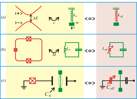
Figure 1: (Color online) Qubit (quantum two-level system) coupled to a classical resonator. (a) Schematic diagram of the model qubit-resonator system. The qubit is represented by the two-level system with the two states, $\left|-\right\rangle$ and $\left|+\right\rangle\,$, and with the energy difference $\Delta E$. The resonator is demonstrated as the spring oscillator with the elasticity coefficient $k_{0}$. As described in the main text, influence of the qubit on the resonator can be described by introducing the effective elasticity coefficient $k_{\mathrm{eff}}$, which includes the qubit’s-state-dependent (or, parametric, for brevity) elasticity coefficient $k_{\mathrm{q}}$. (b) The flux qubit coupled via the mutual inductance $M$ to the $LC$ resonator. This can be described by introducing effective qubit’s-state-dependent inductance $L_{\mathrm{eff}}$, which includes the parametric inductance $L_{\mathrm{q}}$ in parallel to the tank’s inductance $L_{0}$. (c) The impact of the charge qubit on the nanomechanical resonator’s state can be described by introducing the effective qubit’s-state-dependent capacitance $C_{\mathrm{eff}}$, which includes the parametric capacitance $C_{\mathrm{q}}$ in parallel to the resonator’s capacitance $C_{0}$.

The displacement $x$ is the solution of the motion equation

$$m\frac{d^{2}x}{dt^{2}}+\lambda_{0}\frac{dx}{dt}+k_{0}x=\epsilon F_{\mathrm{q}}\left(x,\frac{dx}{dt}\right)+\epsilon F_{\mathrm{p}}\sin\omega_{\mathrm{p}}t.$$ (1)

The oscillations in the nonlinear system described by Eq. (1) can be reduced to oscillations in an equivalent linear system by making use of the Krylov-Bogolyubov technique of asymptotic expansion Bogolyubov . Specifically, in the first-order approximation with respect to a qubit-resonator coupling parameter and close to the principal resonance, $\omega_{\mathrm{p}}\approx\omega_{0}$, the equivalent linear system is characterized by the effective amplitude-dependent elasticity coefficient $k_{\mathrm{eff}}(v)$ and the effective damping factor $\lambda_{\mathrm{eff}}(v)$ (see chapter 7 in Ref. Bogolyubov ):

$$m\frac{d^{2}x}{dt^{2}}+\lambda_{\mathrm{eff}}(v)\frac{dx}{dt}+k_{\mathrm{eff}}(v)x=\epsilon F_{\mathrm{p}}\sin\omega_{\mathrm{p}}t,$$ (2)

$$x = v\cos(\omega_{\mathrm{p}}t+\delta),$$ (3)

$$k_{\mathrm{eff}}(v) = k_{0}-\frac{\epsilon}{\pi v}\int\limits_{0}^{2\pi}\widetilde{F}_{\mathrm{q}}(v,\psi)\cos\psi d\psi\equiv k_{0}+k_{\mathrm{q}},$$ (4)

$$\lambda_{\mathrm{eff}}(v) = \lambda_{0}+\frac{\epsilon}{\pi v\omega_{0}}\int\limits_{0}^{2\pi}\widetilde{F}_{\mathrm{q}}(v,\psi)\sin\psi d\psi\equiv\lambda_{0}+\lambda_{\mathrm{q}},$$ (5)

where $\widetilde{F}_{\mathrm{q}}(v,\psi)\equiv F_{\mathrm{q}}\left(x,\frac{dx}{dt}\right)=F_{\mathrm{q}}\left(v\cos\psi,-\omega_{\mathrm{p}}v\sin\psi\right)$. Note that in Eq. (2) both $v$ and $\delta$ are time-dependent values.

Here, in equations (4) and (5), we have introduced the parametric elasticity coefficient $k_{\mathrm{q}}$ and damping factor $\lambda_{\mathrm{q}}$. In this context the adjective quantum is sometimes used instead of “parametric” to emphasize that it is the qubit-state-dependent, i.e. it is defined by the quantum properties of the coupled system. In what follows, by simply changing the notations we will see that the parametric elasticity coefficient gives either parametric inductance or parametric capacitance, when coupling is inductive or capacitive respectively, while the parametric damping factor will give us the parametric resistance. Note that in equations (4) and (5) the parametric terms $k_{\mathrm{q}}$ and $\lambda_{\mathrm{q}}$ are of the first order in the small parameter of the problem $\epsilon$.

This linearization procedure allows to obtain important information even without solving equations of motion. In particular, the effective resonance frequency of the linearized system $\omega_{\mathrm{eff}}=\sqrt{k_{\mathrm{eff}}/m}$ gives the expression for the frequency shift

$$\Delta\omega=\omega_{\mathrm{eff}}-\omega_{0}=\frac{k_{\mathrm{q}}}{2m\omega_{0}}.$$ (6)

For physical interpretations it is important to emphasize that the application of the linearization technique resulted in the substitution of the nonlinear force by the linear one:

$$\digamma\equiv\epsilon F_{\mathrm{q}}\left(x,\frac{dx}{dt}\right)\longrightarrow\digamma_{\mathrm{q}}=-k_{\mathrm{q}}x-\lambda_{\mathrm{q}}\frac{dx}{dt}.$$ (7)

This latter “parametric” force describes the work done by the quantum system over the resonator; the respective energy transfer during one period is the following

$$W=\int\limits_{0}^{2\pi/\omega_{\mathrm{p}}}\digamma_{\mathrm{q}}\frac{dx}{dt}dt=-\pi\omega_{\mathrm{p}}v^{2}\lambda_{\mathrm{q}}.$$ (8)

This, in dependence on the sign of the parametric damping factor $\lambda_{\mathrm{q}}$, describes periodical extraction or pumping of the energy by the quantum system out of or into the resonator. This is known as the Sisyphus damping and amplification Grajcar08 .

The solution of equation (2) in the first approximation in $\epsilon$ is given by the expression (3) with the amplitude $v=v(t)$ and the phase shift $\delta=\delta(t)$ slowly varying in time. For these values the asymptotic expansion method gives the following system of equations (see chapter 15 in Ref. Bogolyubov )

$$\frac{dv}{dt} = -\frac{\lambda_{\mathrm{eff}}(v)}{2m}v-\frac{\epsilon F_{\mathrm{p}}}{m(\omega_{0}+\omega_{\mathrm{p}})}\cos\delta,$$ (9)

$$\frac{d\delta}{dt} = \omega_{\mathrm{eff}}(v)-\omega_{\mathrm{p}}+\frac{\epsilon F_{\mathrm{p}}}{mv(\omega_{0}+\omega_{\mathrm{p}})}\sin\delta.$$ (10)

In the regime of stationary oscillations: $dv/dt=d\delta/dt=0$, and we obtain equations for the amplitude $v$ and the phase shift $\delta$, which can be written in the form

$$\tan\delta = \frac{k_{\mathrm{q}}(v)}{\omega_{0}\lambda_{\mathrm{eff}}(v)},$$ (11)

$$v = -\frac{\epsilon F_{\mathrm{p}}\cos\delta}{\omega_{0}\lambda_{\mathrm{eff}}(v)}.$$ (12)

In what follows it will be demonstrated that the phase shift $\delta$ and the amplitude $v$ can be directly observed experimentally, which gives the information about the quantum system through the values of the parametric elasticity coefficient $k_{\mathrm{q}}$ and damping factor $\lambda_{\mathrm{q}}$.

II.2 Inductive coupling with $LCR$ resonator. Parametric inductance

Now we consider as an illustrative case the system of a flux qubit (with geometrical inductance $L$ and average current $I_{\mathrm{qb}}$) coupled inductively to the $LCR$ tank circuit, as shown in Fig. 2. The approach, presented here, is the development of the theory in Refs. Rifkin76 ; Greenberg02b ; Smirnov03 . The quantum system is considered to be weakly coupled via a mutual inductance $M$ to the classical tank circuit. The circuit consists of the inductor $L_{0}$, capacitor $C_{0}$, and the resistor $R_{0}$ connected, for the specification, in parallel. The tank circuit is biased by the current $I_{\mathrm{bias}}$, and the voltage on it $V$ can be measured.

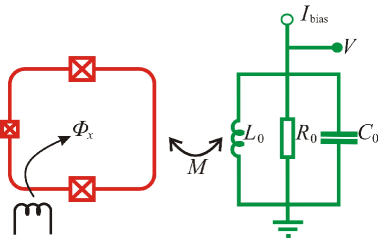
Figure 2: (Color online) Flux qubit coupled inductively to an $LCR$ (tank) circuit. The flux qubit is pierced by the magnetic flux $\Phi_{x}$ induced by the current in the controlling coil and by the current in the tank’s inductor. The qubit is coupled via the mutual inductance $M$ to the tank circuit. The resonant tank circuit consists of the inductor $L_{0}$, capacitor $C_{0}$, and resistor $R_{0}$; the circuit is biased with an RF current $I_{\mathrm{bias}}$. The tank voltage $V$ is the measurable value.

The flux qubit can be described by the pseudospin Hamiltonian Mooij99

$$H = -\frac{\Delta}{2}\sigma_{x}-\frac{\varepsilon(t)}{2}\sigma_{z},$$ (13)

$$\varepsilon(t) = \varepsilon_{0}+A\sin\omega t,$$ (14)

where the diagonal term $\varepsilon$ is the energy bias, the off-diagonal term $\Delta$ is the tunneling amplitude between the wells (which corresponds to the definite directions of the current in the loop) and $\sigma_{x,z}$ are the Pauli matrices.

To obtain the equation for the tank circuit voltage, we write down the system of equations for the current in the three branches, namely, through the inductor ($I_{\mathrm{L}}$), the capacitor ($I_{\mathrm{C}}$), and the resistor ($I_{\mathrm{R}}$) (in particular, for systems with superconducting elements see e.g. Ref. Likharev ):

$$I_{\mathrm{bias}} = I_{\mathrm{L}}+I_{\mathrm{C}}+I_{\mathrm{R}},$$ (15)

$$I_{\mathrm{C}} = C_{0}\overset{\cdot}{V},\text{ }I_{\mathrm{R}}=V/R_{0},$$ (16)

$$V = L_{0}\dot{I}_{\mathrm{L}}-\dot{\Phi}_{\mathrm{e}},$$ (17)

where $\Phi_{\mathrm{e}}$ is the flux through the inductor of the tank circuit. This flux is the response of the quantum system to the flux, induced in it by the current $I_{\mathrm{L}}$. It follows that the voltage $V$ in the current-biased tank circuit ($I_{\mathrm{bias}}=I_{\mathrm{A}}\sin\omega_{\mathrm{p}}t$) is described by the following nonlinear equation

$$C_{0}\frac{d^{2}V}{dt^{2}}+R_{0}^{-1}\frac{dV}{dt}+L_{0}^{-1}V=-\frac{\dot{\Phi}_{\mathrm{e}}(V,\dot{V})}{L_{0}}+I_{\mathrm{A}}\omega_{\mathrm{p}}\cos\omega_{\mathrm{p}}t.$$ (18)

The external flux $\Phi_{\mathrm{e}}$ is assumed to be proportional to the coupling parameter $k^{2}=M^{2}/LL_{0}\ll 1$ and to depend on time via the voltage $V$ and its time derivative $\dot{V}$. Equation (18) for the voltage $V$ coincides with the nonlinear equation (1) for the variable $x$ with obvious change of the notations.

Thus, the formalism presented in the previous subsection is directly applicable for the given problem. Specifically, in the first order approximation with respect to the coupling parameter $k^{2}$ and close to the principal resonance ($\omega_{\mathrm{p}}\approx\omega_{0}\equiv 1/\sqrt{L_{0}C_{0}}$), the equivalent linear system is characterized by the effective resistance $R_{\mathrm{eff}}$ and inductance $L_{\mathrm{eff}}$ as following

$$C_{0}\frac{d^{2}V}{dt^{2}}+R_{\mathrm{eff}}^{-1}\frac{dV}{dt}+L_{\mathrm{eff}}^{-1}V=I_{A}\omega_{\mathrm{p}}\cos\omega_{\mathrm{p}}t,$$ (19)

$$V = v\cos(\omega_{\mathrm{p}}t+\delta),$$ (20)

$$\frac{1}{R_{\mathrm{eff}}(v)} = \frac{1}{R_{0}}+\frac{1}{R_{\mathrm{q}}(v)},$$ (21)

$$\frac{1}{L_{\mathrm{eff}}(v)} = \frac{1}{L_{0}}+\frac{1}{L_{\mathrm{q}}(v)}.$$ (22)

Here $Q_{0}=\omega_{0}C_{0}R_{0}$ is the quality factor of the unloaded tank circuit (at $\Phi_{\mathrm{e}}=0$) and the parametric (qubit’s-state dependent) resistance $R_{\mathrm{q}}$ and inductance $L_{\mathrm{q}}$ are given by the formulas

$$\frac{1}{R_{\mathrm{q}}(v)} = -\frac{Q_{0}}{\pi vR_{0}}\int\limits_{0}^{2\pi}\widetilde{\dot{\Phi}}_{\mathrm{e}}(v,\psi)\sin\psi d\psi,$$ (23)

$$\frac{1}{L_{\mathrm{q}}(v)} = \frac{1}{\pi vL_{0}}\int\limits_{0}^{2\pi}\widetilde{\dot{\Phi}}_{\mathrm{e}}(v,\psi)\cos\psi d\psi,$$ (24)

where $\widetilde{\dot{\Phi}}_{\mathrm{e}}(v,\psi)\equiv\dot{\Phi}_{\mathrm{e}}(V,\dot{V})=\dot{\Phi}_{\mathrm{e}}(v\cos\psi,-v\omega_{\mathrm{p}}\sin\psi)$. The resonant frequency $\omega_{\mathrm{eff}}$ becomes amplitude-dependent and is shifted by

$$\Delta\omega=\omega_{\mathrm{eff}}(v)-\omega_{0}=\frac{\omega_{0}L_{0}}{2L_{\mathrm{q}}(v)}.$$ (25)

The phase shift $\delta$ and the amplitude $v$ depend on the probing frequency detuning $\xi_{0}\equiv\frac{\omega_{0}-\omega_{\mathrm{p}}}{\omega_{0}}$ and the qubit state (via $L_{\mathrm{q}}$ and $R_{\mathrm{q}}$). In the stationary regime they are given by the solution of the system of equations

$$\left\{\begin{array}[]{c}\tan\delta=2Q_{0}\frac{R_{\mathrm{eff}}}{R_{0}}\left(\xi_{0}+\frac{L_{0}-L_{\mathrm{eff}}}{2L_{0}}\right),\\ v=I_{A}R_{\mathrm{eff}}\cos\delta,\end{array}\right.$$ (26)

which can also be rewritten alternatively in terms of the effective quality factor $Q_{\mathrm{eff}}=\omega_{0}C_{0}R_{\mathrm{eff}}(v)$ and effective frequency shift $\xi_{\mathrm{eff}}=\left[\omega_{\mathrm{eff}}(v)-\omega_{\mathrm{p}}\right]/\omega_{0}$.

Thus, the observable values – the amplitude $v$ and the phase shift $\delta$ – are defined by equations (26), which depend on the response of the measurable system, $\Phi_{e}(V,\dot{V})$. As we discussed above, strictly speaking, the dynamics of the tank circuit has to be considered jointly with the dynamics of the qubit (corresponding calculations see e. g. in Greenberg08 ). However, in what follows we consider two illustrative limiting cases, when the dynamics of the qubit can be treated separately from the dynamics of the tank circuit. For simplification we introduce phenomenologically the relaxation time $T_{1}$ which is caused by the coupling to the environment and to the tank as well.

1. Low-quality qubit ($T_{1}\ll T$): phase shift probes the parametric inductance of qubit.

First case which allows to detach the equations for the qubit and resonator, is when all the qubit’s characteristic times, and in particular the relaxation time $T_{1}$, are smaller than the tank’s period $T=2\pi/\omega_{0}$. Then the equations for the tank voltage can be averaged over the period of fast oscillations. Then the time derivative of the flux $\Phi_{e}$, induced by the qubit in the tank circuit can be described as

$$\dot{\Phi}_{e}=M\dot{I}_{\mathrm{qb}}=M\frac{\partial I_{\mathrm{qb}}}{\partial\Phi}\dot{\Phi},$$ (27)

where $\Phi=\Phi_{\mathrm{dc}}+MI_{\mathrm{L}}$ is the flux in the qubit’s loop, which consists of the time-independent part $\Phi_{\mathrm{dc}}$ and of the flux, induced by the current $I_{\mathrm{L}}$ in the tank’s inductor. This can be rewritten by introducing the effective inductance of the qubit, $\mathcal{L}^{-1}=\partial I_{\mathrm{qb}}(\Phi)/\partial\Phi$, and the characteristic inductance value $\widetilde{L}=M^{2}\mathcal{L}^{-1}$. Then $\dot{\Phi}_{e}=\widetilde{L}(I_{\mathrm{L}})\dot{I}_{\mathrm{L}}$ and for the tank voltage we have $V=L_{0}\dot{I}_{\mathrm{L}}-\dot{\Phi}_{e}=(L_{0}-\widetilde{L}(I_{\mathrm{L}}))\dot{I}_{\mathrm{L}}$. In the first approximation in $k^{2}$ in the expression $\dot{\Phi}_{e}=\widetilde{L}(I_{\mathrm{L}})\dot{I}_{\mathrm{L}}$ we can insert $I_{\mathrm{L}}$ found from this equation

$$I_{\mathrm{L}}(t)\approx\frac{1}{L_{0}}\int Vdt\approx\frac{v}{\omega_{0}L_{0}}\sin(\omega_{\mathrm{p}}t+\delta).$$ (28)

Then from Eqs. (23-24) we have $R_{\mathrm{q}}^{-1}=0$ (hence $R_{\mathrm{eff}}=R_{0}$) and

$$\frac{L_{0}}{L_{\mathrm{q}}}=\frac{k^{2}L}{\pi}\int\limits_{0}^{2\pi}\mathcal{L}^{-1}(v,\psi)\cos^{2}\psi d\psi,$$ (29)

where the qubit’s effective inductance is defined by the total flux $\Phi$, piercing the qubit’s loop

$$\mathcal{L}^{-1}(v,\psi)\equiv\left.\frac{\partial I_{\mathrm{qb}}(\Phi)}{\partial\Phi}\right|_{\Phi=\Phi_{\mathrm{dc}}+\frac{M}{L_{0}\omega_{0}}v\sin\psi}.$$ (30)

Then for the phase shift $\delta$ and the voltage amplitude $v$ we obtain Shevchenko08

$$\tan\delta\approx 2Q_{0}\xi_{0}+Q_{0}\frac{L_{0}}{L_{\mathrm{q}}},\text{ \ }v\approx I_{A}R_{0}\cos\delta,$$ (31)

which is the generalization of the result of Ref. Greenberg02a for the case when the qubit can be in the superpositional state, which is taken into account here by the expectation value of the current $I_{\mathrm{qb}}$. If the bias current amplitude $I_{A}$ is small enough to be ignored in Eq. (30), then

$$L_{\mathrm{q}}^{-1} = k^{2}\frac{L}{L_{0}}\mathcal{L}^{-1},\text{ \ \ \ \ \ }\mathcal{L}^{-1}\approx\frac{\partial I_{\mathrm{qb}}}{\partial\Phi_{\mathrm{dc}}},$$

$$\tan\delta \approx 2Q_{0}\xi_{0}+k^{2}Q_{0}L\mathcal{L}^{-1},\text{ \ }v\approx I_{A}R_{0}\cos\delta.$$ (32)

At the resonant frequency $\xi_{0}=0$, the phase shift $\delta$ is proportional to the inverse inductance of the qubit $\mathcal{L}^{-1}$. Here it is worthwhile to emphasize the expression for the parametric inductance, which is expressed via the derivative of the expectation value of the current in the qubit’s loop $I_{\mathrm{qb}}=-I_{\mathrm{p}}\left\langle\sigma_{z}\right\rangle$,

$$L_{\mathrm{q}}^{-1}=-L_{0}^{-1}k^{2}\frac{LI_{\mathrm{p}}}{\Phi_{0}}\frac{\partial\left\langle\sigma_{z}\right\rangle}{\partial f_{\mathrm{dc}}}.$$ (33)

2. Higher-quality qubit ($T_{1}\lesssim T$): parametric resistance due to qubit’s lagging.

Another illustrative situation, where the qubit’s dynamics can be considered separately from the resonator’s one, is the case when the qubit relaxation time $T_{1}$ is of the same order as the tank’s period $T$, namely, $T_{1}\lesssim T$. The qubit’s response to the resonator probing signal can be phenomenologically described by introducing the lagging time $t^{\prime}=t-T_{1}$, so that instead of Eq. (27) we have

$$\dot{\Phi}_{e}(t)=\widetilde{L}(I_{\mathrm{L}}(t^{\prime}))\dot{I}_{\mathrm{L}}(t^{\prime}).$$ (34)

In this way, the qubit’s response depends on the current in the tank $I_{\mathrm{L}}=I_{\mathrm{L}}(t^{\prime})$, which is given by

$$I_{\mathrm{L}}(t^{\prime})\approx\frac{v}{\omega_{0}L_{0}}\left(C\sin(\omega_{\mathrm{p}}t+\delta)-S\cos(\omega_{\mathrm{p}}t+\delta)\right)$$ (35)

with $S=\sin(\omega_{\mathrm{p}}T_{1})$ and $C=\cos(\omega_{\mathrm{p}}T_{1})$. For the small bias current Eqs. (21-22) and (34-35) result in the following expressions for the parametric inductance and resistance

$$L_{0}/L_{\mathrm{q}} \approx C\cdot k^{2}L\mathcal{L}^{-1},$$

$$R_{0}/R_{\mathrm{q}} \approx-S\cdot k^{2}Q_{0}L\mathcal{L}^{-1}.$$ (36)

By analogy with Eq. (33), the latter phenomenological equation can be rewritten in the form explicitly demonstrating its quantum character,

$$R_{\mathrm{q}}^{-1}=S\frac{k^{2}Q_{0}}{R_{0}}\frac{LI_{\mathrm{p}}}{\Phi_{0}}\frac{\partial\left\langle\sigma_{z}\right\rangle}{\partial f_{\mathrm{dc}}}.$$ (37)

By making use of Eq. (8), we obtain that the energy transferred from qubit into the resonator (or, out of the resonator, for the opposite sign) during one period is

$$W=-\pi\omega_{\mathrm{p}}v^{2}R_{\mathrm{q}}^{-1}.$$ (38)

We emphasize here that both the parametric inductance and resistance in Eq. (36) are proportional to the qubit’s inductance $\mathcal{L}$. Then, one obtains equations for $\delta$ and $v$, which are simplified in the first approximation in $k^{2}Q_{0}L\mathcal{L}^{-1}$. In this case for the probing frequency equal to the resonant one, $\xi_{0}=0$, the resulting formulas are

$$\tan\delta \approx C\cdot k^{2}Q_{0}L\mathcal{L}^{-1},$$ (39)

$$\frac{v}{I_{A}R_{0}} \approx 1+S\cdot k^{2}Q_{0}L\mathcal{L}^{-1}.$$

Note that both the phase shift and amplitude are related to the qubit’s effective inductance $\mathcal{L}$, which explains their similar behavior in experiment. These equations are useful for the analysis of the experimental results, as it will be demonstrated in Section 4.

II.3 Capacitive coupling with nanomechanical resonator. Parametric capacitance

Consider now the charge qubit capacitively coupled to a resonator. In this case, like in the one considered above, the resonator can be the tank circuit. Alternatively, the resonator can be a nanomechanical resonator (NR), as in Ref. LaHaye09 . For the illustrative purpose, we consider here this latter case.

The split-junction charge qubit (shown in red in Fig. 3) consists of a small island between two Josephson junctions (also called Cooper-pair box), whose state is controlled by the magnetic flux $\Phi$ and the gate voltage $V_{\mathrm{CPB}}+V_{\mathrm{MW}}$. Here $V_{\mathrm{CPB}}$ is the dc voltage used to tune the energy levels of the qubit and $V_{\mathrm{MW}}=V_{\mu}\sin\omega t$ is the microwave signal used to change the energy-level occupations. The driven Cooper-pair box is described in the two-level approximation by the Hamiltonian in the “charge” representation, Eqs. (13-14), where the tunnel splitting $\Delta$ is equal to the Josephson energy controlled by the magnetic flux $\Phi$: $\Delta=E_{\mathrm{J}0}\left|\cos(\pi\Phi/\Phi_{0})\right|$. The charging energy and the driving amplitude are the following $\varepsilon_{0}=-8E_{\mathrm{C}}(n_{\mathrm{g}}-1/2)$ and $A=-8E_{\mathrm{C}}n_{\mathrm{\mu}}$, where the Coulomb energy $E_{\mathrm{C}}=e^{2}/2C_{\Sigma}$ is defined by the total capacitance $C_{\Sigma}=2C_{\mathrm{J}}+C_{\mathrm{CPB}}+C_{\mathrm{NR}}$ and the effective Josephson capacitance is introduced $2C_{\mathrm{J}}\equiv C_{\mathrm{J}1}+C_{\mathrm{J}2}$, the dimensionless driving amplitude $n_{\mu}=C_{\mathrm{CPB}}V_{\mu}/2e$. The dimensionless polarization charge $n_{\mathrm{g}}=n_{\mathrm{NR}}+n_{\mathrm{CPB}}$ is the fractional part of the respective polarization charges in two capacitances: $n_{\mathrm{NR}}=\left\{C_{\mathrm{NR}}V_{\mathrm{NR}}/2e\right\}$ and $n_{\mathrm{CPB}}=\left\{C_{\mathrm{CPB}}V_{\mathrm{CPB}}/2e\right\}$.

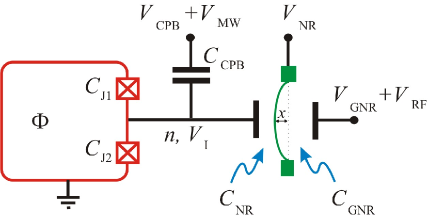
Figure 3: (Color online) Charge qubit probed by a nanomechanical resonator. The charge qubit is the Cooper-pair box, controlled by the magnetic flux $\Phi$ and the gate voltage $V_{\mathrm{CPB}}+V_{\mathrm{MW}}$. The resonator probing the qubit’s state here is the NR, which is characterized by the displacement at the midpoint $x$. The voltage-biased NR is measured through its resonance frequency shift $\Delta\omega_{\mathrm{NR}}$. Shevchenko11

The Cooper-pair box here is formed by four capacitors, $C_{\mathrm{J}1}$, $C_{\mathrm{J}2}$, $C_{\mathrm{CPB}}$, and $C_{\mathrm{NR}}$. One of the plates of the latter capacitor is formed by the NR. The displacement of the NR $x$ is much smaller than the distance $d$ between the plates. Then the capacitance between the NR and the qubit reads

$$C_{\mathrm{NR}}(x)\approx C_{\mathrm{NR}}+\frac{\partial C_{\mathrm{NR}}}{\partial x}x\equiv C_{\mathrm{NR}}\left(1+\frac{x}{\xi}\right).$$ (40)

Here $C_{\mathrm{NR}}$ stands for the capacitance value at the zero displacement. The displacement of the NR influences the qubit through the changes in the polarization charge; to make it significant, a large dc voltage $V_{\mathrm{NR}}$ is applied. On the other side, the NR is biased by dc and rf voltages $V_{\mathrm{GNR}}$ and $V_{\mathrm{RF}}$ through the capacitance $C_{\mathrm{GNR}}$.

One of the approaches to describe the system qubit-resonator is to introduce the parametric capacitance as following (for more details see Ref. Shevchenko11 ). Let us introduce the effective capacitance, as it is demonstrated in Fig. 1(c), by differentiating the charge $Q_{\mathrm{NR}}$ of the capacitor $C_{\mathrm{NR}}$ Sillanpaa05 ; Duty05 ; Johansson06 : $C_{\mathrm{eff}}=\partial Q_{\mathrm{NR}}/\partial V_{\mathrm{NR}}$. Then, for the charge $Q_{\mathrm{NR}}=(V_{\mathrm{NR}}-V_{\mathrm{I}})C_{\mathrm{NR}}$ with the island’s voltage given by $V_{\mathrm{I}}=2e(n_{\mathrm{g}}-\left\langle n\right\rangle)/C_{\Sigma}$, we obtain $C_{\mathrm{eff}}=C_{\mathrm{geom}}+C_{\mathrm{q}}$, which consists of the parametric capacitance

$$\text{ }C_{\mathrm{q}}=\frac{C_{\mathrm{NR}}^{2}}{C_{\Sigma}}\frac{\partial\left\langle n\right\rangle}{\partial n_{\mathrm{g}}}$$ (41)

and the geometric capacitance $C_{\mathrm{geom}}$

$$C_{\mathrm{geom}}=\frac{C_{\mathrm{NR}}(C_{\Sigma}-C_{\mathrm{NR}})}{C_{\Sigma}}\approx\frac{2C_{\mathrm{J}}C_{\mathrm{NR}}}{2C_{\mathrm{J}}+C_{\mathrm{NR}}}\approx C_{\mathrm{NR}},\text{ }$$ (42)

where the approximations are valid for $C_{\mathrm{CPB}}\ll C_{\mathrm{J}},C_{\mathrm{NR}}$ and $C_{\mathrm{NR}}\ll C_{\mathrm{J}}$ respectively. Then one can consider the force $F_{\mathrm{NR}}$, which acts on the NR from the left electrode, as the electrostatic force from the effective capacitance [see Fig. 1(c)]: $F_{\mathrm{NR}}=\frac{1}{2}\frac{\partial}{\partial x}\left(C_{\mathrm{eff}}V_{\mathrm{NR}}^{2}\right)$. Then the term with the parametric capacitance, in which $C_{\mathrm{NR}}^{2}\approx C_{\mathrm{NR}}^{2}\left(1+x/\xi\right)^{2}$, results in the following resonance frequency shift of the NR

$$\frac{\Delta\omega_{\mathrm{NR}}}{\omega_{\mathrm{NR}}} = -\frac{\beta C_{\mathrm{\Sigma}}}{C_{\mathrm{NR}}^{2}}C_{\mathrm{q}}=-\beta\frac{\partial\left\langle n\right\rangle}{\partial n_{\mathrm{g}}}=-\frac{\beta}{2}\frac{\partial\left\langle\sigma_{z}\right\rangle}{\partial n_{\mathrm{g}}},$$ (43)

$$\beta = \frac{1}{m\omega_{\mathrm{NR}}^{2}C_{\Sigma}}\left(\frac{C_{\mathrm{NR}}V_{\mathrm{NR}}}{\xi}\right)^{2}.$$

We would like to note that the results obtained for the system qubit-NR can be definitely extended to other systems. For example the charge qubit can be coupled to a tank circuit instead of a NR. In contrast to the inductive coupling, considered in the previous subsection, here we mean capacitive coupling. Then it is straightforward to obtain the expression for the measurable value, the tank circuit phase shift at resonance frequency, $\xi_{0}=0$, Shevchenko11

$$\tan\delta\approx Q_{0}\frac{C_{\mathrm{q}}}{C_{0}},$$ (44)

cf. Eq. (31), where the phase shift probes the parametric inductance. In section 4 it will be demonstrated how these expressions can be used for the description of the realistic system.

III 3. Dynamical behavior of a two-level system

Application of the semiclassical theory, presented in the previous subsection, to the description of the qubits-resonator system makes possible to separate the slow dynamics of the resonator from the fast dynamics of the qubits system. This allows to consider first the dynamics of a qubit or a system of qubits. Then, the resonator can monitor the state of the system of qubits. In this section we will outline the description of the multiphoton processes in a qubit, while the presentation of the specific results is the subject of the next two sections.

Initialization and manipulation of the qubit’s systems require certain external signals. The principal features of the driven system are captured for the harmonic driving, Eq. (14), to which we limit our consideration. Different theoretical approaches can be used for a driven two-level system, which is described in the books and reviews Blum ; Weiss ; Faisal ; Nakamura02 ; Grifoni98 ; Chu04 . The choice of the formalism depends on the formulation of a problem and on the parameters of the system, such as the bias offset $\varepsilon_{0}$, driving amplitude $A$ and frequency $\omega$. The clear description can be given for the temporal dynamics in the so-called adiabatic-impulse model, where the driven evolution is considered adiabatic far from the avoided-level crossings with the impulse-type Landau-Zener transitions, when the energy distance is minimal Garraway97 ; Forre04 ; Shevchenko10 . As the result of this theory, the overall dynamics is described by the long-time Rabi-type oscillations of the level occupation probabilities with the step-like features due to the Landau-Zener transitions.

Another technique, which can be more convenient for the resonant driving, is the rotating wave approximation (RWA) Son09 ; Wen09 ; Ferron10 . It consists in neglecting the rapidly oscillating (non-resonant) terms. The common approach for making use of this approximation is taking small driving amplitudes, $A\ll\Delta E$. Then, the first-order consideration gives usual Rabi oscillations of the level occupation probabilities close to the position of the one-photon resonance, where $\omega\approx\Delta E/\hbar$. In the $k$-th approximation, the resonant excitation appears close to the parameters, where the energy of $k$ photons matches the qubit’s energy distance Coh-Tan ; Delone

$$k\hbar\omega=\Delta E.$$ (45)

The time evolution is described by the multiphoton Rabi oscillations Shirley65 , while the time-averaged upper-level occupation probability has the Lorentzian shape with the maximum equal to $1/2$ at the exact resonance defined by Eq. (45).

With increasing the driving amplitude the resonances shift Krainov80 from their positions given by the perturbation theory and defined by the exact multiphoton relation (45). The first-order correction to the position of the resonances is the so-called Bloch-Siegert shift Coh-Tan ; it was demonstrated for the superconducting qubits in Ref. Tuorila10 . Thus, in general, the position of the multiphoton resonances is amplitude-dependent.

For the description of the strongly driven qubits, another formulation of the RWA can be used. There, the minimal energy level splitting $\Delta$ is the small parameter, namely, it is assumed $\Delta\ll\sqrt{A\omega}$ LopezCastillo92 ; Oliver05 ; Ashhab07 . Then the $k$-photon excitation appears close to the resonant parameters, given by the relation $\varepsilon_{0}=k\hbar\omega$. There, the upper-level occupation probability $P_{\mathrm{up}}(t)$ oscillates with the frequency $\Omega_{\mathrm{R}}=\sqrt{(\varepsilon_{0}-k\hbar\omega)^{2}+\Delta_{k}^{2}}$ with the renormalized splitting $\Delta_{k}=\Delta J_{k}\left(A/\omega\right)$; $J_{k}$ is the Bessel function. The time-averaged probability in the vicinity of the $k$-th resonance is given by

$$\overline{P}_{\mathrm{up}}=\frac{1}{2}\frac{\Delta_{k}^{2}}{(\varepsilon_{0}-k\hbar\omega)^{2}+\Delta_{k}^{2}}.$$ (46)

Being time averaged, the Rabi oscillations are described by the Lorentzian dependence of the upper-level occupation on the system’s parameters (the bias or the driving frequency) Tornes08 . Here arises an interesting and important problem of distinction of the respective quantum oscillations from their classical counterparts, which are the parametric resonances. This was the subject of Refs. Gronbech05 ; Marchese07 ; ShevchenkoOZ08 .

The most straightforward approach for the numerical description of the dynamics of a two-level system is the solution of the Schrödinger equation Shevchenko05 . Then, the influence of the dissipation can be taken into account phenomenologically by introducing energy and phase relaxation times, $T_{1}$ and $T_{2}$, and solving the respective Bloch equation Blum . Instead, in the more general approach, the dissipative environment can be described as an ensemble of oscillators, which would result in the Bloch-Redfield equation for the reduced density matrix Leggett87 ; Goorden05 . This latter formalism will be demonstrated in Sec. 5 being applied to the specific case of the two-qubit system.

Note that the multiphoton transitions can also be driven by the bichromatic field, when the energy level distance $\Delta E$ is matched by the energy of several photons of one (say, microwave-) frequency plus several photons of another (say, radio-) frequency. Such transitions were studied both in microscopic systems Delone ; Saiko07 , and in the Josephson-junction qubits Saito06 ; Gunnarsson08 ; Paila09 . Also for the case of a flux qubit it was demonstrated that the persistence of Rabi oscillations can be supported by either the low-frequency signal Greenberg05 or induced by noise Omelyanchouk09 .

IV 4. Excitation of a superconducting qubit

Let us get back to the qubit-resonator systems. In the previous Section we have discussed a modification of the qubit states (and therefore its observables) under different types of excitations. A natural next step is to analyze the corresponding (via qubits) change of the resonator properties. In this section we demonstrate this by presenting respective theoretical results for different realizations of the qubit-resonator systems, making use of the theory presented in the previous two sections. The emphasis is made on demonstrating the consistency of the theoretical results with the experimental ones.

IV.1 Inductance of superconducting qubits

Consider a qubit biased with a DC flux $\Phi_{\mathrm{dc}}$ and driven with an AC flux $\Phi_{\mathrm{ac}}\sin\omega t$, introducing $f_{\mathrm{dc}}=\Phi_{\mathrm{dc}}/\Phi_{0}-1/2$ and $f_{\mathrm{ac}}=\Phi_{\mathrm{ac}}/\Phi_{0}.$ In order to get the effective inductance $\mathcal{L}$, as defined by Eq. (30), we have to calculate the average current in the qubit: $I_{\mathrm{qb}}=\left\langle I\right\rangle=\mathrm{Tr}\left(\rho I\right)$, where $I=I_{\mathrm{p}}\sigma_{z}$ is the current operator defined with the amplitude $I_{\mathrm{p}}$ and the Pauli matrix $\sigma_{z}$. We calculate the reduced density matrix $\rho$ with the Bloch equations Blum ; Shevchenko05 which include phenomenological relaxation times, $T_{1}$ and $T_{2}$. It is convenient to express the density matrix in the energy representation: $\rho=\left(1/2\right)\left(\tau_{0}+X\tau_{x}+Y\tau_{y}+Z\tau_{z}\right)$, where $\tau_{i}$ are the Pauli matrices for this basis and $\tau_{0}$ stands for the unity matrix. The value $Z=\left\langle\widehat{\tau}_{z}\right\rangle$ is equal to the difference between the populations of the ground and excited states.

Let us find now the explicit expressions for the effective qubit’s inductance for both the interferometer-type (split-junction) charge qubit Krech02 ; Zorin02 and flux qubit Mooij99 . For the interferometer-type charge qubit, as considered in detail in Ref. Shnyrkov06 , the circulating current $I_{0}$ is flux-dependent and Eqs. (32) show that there are two terms contributing in the tank circuit’s phase shift,

$$\tan\delta\approx\frac{k^{2}QL}{\Phi_{0}}\left(\frac{\partial I_{0}}{\partial f_{\mathrm{dc}}}Z+I_{0}\frac{\partial Z}{\partial f_{\mathrm{dc}}}\right).$$ (47)

In a classical system (where the current has a definite direction) or in the ground state, the difference between the energy level’s populations is constant, $Z=const$, and the second term in Eq. (47) is zero. In contrast, for the quantum system the interplay between these two terms is essential. At this point it is worthwhile to notice that the second term can dominate at resonant excitation, as it was the case in the work Shnyrkov06 (see also below). This means that the second (“quantum”) term can significantly increase the sensitivity of the impedance measurement technique, as compared to the classical situation described by the first term in Eq. (47).

Consider now the case of a flux qubit. The current operator is defined in the flux basis Mooij99 , $I=I_{\mathrm{p}}\sigma_{z}$, where $I_{\mathrm{p}}$ stands for the amplitude value of the persistent current, and hence the value $\left\langle\sigma_{z}\right\rangle$ defines the difference between the probabilities of the clockwise and counter-clockwise current directions in the loop: $\left\langle\sigma_{z}\right\rangle=P_{\downarrow}-P_{\uparrow}=2P_{\downarrow}-1$. Then with Eqs. (32) we obtain

$$\tan\delta\approx k^{2}Q\frac{LI_{\mathrm{p}}}{\Phi_{0}}2\frac{\partial P_{\downarrow}}{\partial f_{\mathrm{dc}}}.$$ (48)

In the energy representation we rewrite Eq. (48)

$$\tan\delta\approx k^{2}Q\frac{LI_{\mathrm{p}}}{\Phi_{0}}\frac{\partial}{\partial f_{\mathrm{dc}}}\left(\frac{\Delta}{\Delta E}X-\frac{I_{\mathrm{p}}\Phi_{0}f_{\mathrm{dc}}}{\Delta E}Z\right).$$ (49)

Here $\Delta E=\sqrt{\Delta^{2}+(I_{\mathrm{p}}\Phi_{0}f_{\mathrm{dc}})^{2}}$ is the distance between the stationary energy levels.

After the time-averaging over the driving period $2\pi/\omega$, this expression is written as following

$$\tan\delta\approx-k^{2}Q\frac{LI_{\mathrm{p}}^{2}}{\Delta}\left(\frac{\Delta^{3}}{\Delta E^{3}}+\frac{\Delta}{\Delta E}f_{\mathrm{dc}}\frac{\partial}{\partial f_{\mathrm{dc}}}\right)Z.$$ (50)

If a qubit is resonantly excited with the driving frequency $\omega$, then the partial energy levels occupation probability $Z$ has the Lorentzian-shape dependence on $f_{\mathrm{dc}}$. It follows that the derivative $\partial Z/\partial f_{\mathrm{dc}}$ takes the shape of a hyperbolic-like structure, i.e. it changes from a peak to a dip in the point of the resonance at $\Delta E(f_{\mathrm{dc}})\approx k\hbar\omega$.

IV.2 Equilibrium-state measurement

For the description of the measurement of a flux qubit in the thermal equilibrium one has to put $X=0$ and $Z=\tanh\left(\Delta E/2k_{\mathrm{B}}T\right)$ in Eq. (49),

$$\tan\delta\approx-k^{2}Q\frac{LI_{\mathrm{p}}^{2}}{\Delta}\left(\frac{\Delta^{3}}{\Delta E^{3}}+\frac{\Delta}{\Delta E}f_{\mathrm{dc}}\frac{\partial}{\partial f_{\mathrm{dc}}}\right)\tanh\left(\frac{\Delta E}{2k_{\mathrm{B}}T}\right).$$ (51)

The ground-state measurement at $k_{\mathrm{B}}T\ll\Delta E$ is described with $X=0$ and $Z=1$, which means replacing the hyperbolic tangent in Eq. (51) with the unity. The formula (51) for the ground state obtained by differentiating the probability $P_{\downarrow}$, Eqs. (48-49), coincides with the earlier obtained results (see Eqs. (3-4) in Ref. Ilichev04 ). The resulting tank phase shift is shown in Fig. 4 for the following parameters taken from Ref. Grajcar04 : $\Delta/h=1.3$ GHz, $I_{\mathrm{p}}\Phi_{0}/h=930$ GHz, $\omega_{0}/2\pi=32.675$ MHz, $LI_{\mathrm{p}}/\Phi_{0}=0.0055$, $M/L=0.725$, $Q_{0}=725$, $k=0.02$.

The accurate account of $Z$ in Eq. (51) allows to describe both the suppression and widening of the zero-bias dip (that is at $f_{\mathrm{dc}}=0$) as it was experimentally demonstrated in Ref. Grajcar04 . Indeed, the suppression of the zero-bias dip (at $f_{\mathrm{dc}}=0$) is described by the first term in Eq. (51). The widening is due to the second term that comes from differentiating the hyperbolic tangent; this term becomes relevant for temperatures larger than $\Delta$, and results in the exponential rise of the width for $T>T^{\ast}=\Delta/k_{\mathrm{B}}$, as demonstrated in the inset in Fig. 4.

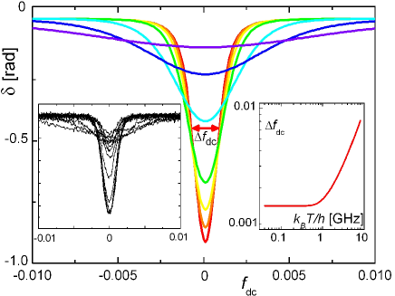
Figure 4: (Color online) The equilibrium-state measurement. The dependence of the tank phase shift on the flux detuning $f_{\mathrm{dc}}=\Phi_{\mathrm{dc}}/\Phi_{0}-1/2$, when the qubit is thermally excited. The curves are plotted for $k_{\mathrm{B}}T/h=0.2$, $0.5$, $0.7$, $1$, $2$, $4$, and $8$ GHz. Left inset: corresponding experimental results Grajcar04 . Right inset: temperature dependence of the width $\Delta f_{\mathrm{dc}}$ of the dip at half-depth in the phase shift, shown in the main panel. ShevchenkoPG08

IV.3 Resonant transitions in the charge qubit

In Ref. Shnyrkov06 the resonant excitation of the interferometer-type (split-junction) charge qubit was demonstrated experimentally and described theoretically. In accordance with the formula (47) one expects the resonances to appear differently when either first or the second term is dominated. To demonstrate this, in Fig. 5 we plot the dependence of the tank circuit phase shift $\delta$ both as the function of the dimensionless bias voltage $n_{\mathrm{g}}=C_{\mathrm{g}}V_{\mathrm{g}}/2e$ and of the dimensionless magnetic flux detuning $f_{\mathrm{dc}}$. For the former case the value $f_{\mathrm{dc}}=0$ was taken, where $I_{0}=0$. This results in disappearance of the second term in Eq. (47), and the resonant excitation of the qubit is visualized with the Lorentzian peaks in Fig. 5(a,b). When the second term is dominant, the multiphoton transitions in the qubit result in the peak-and-dip structures in the dependence of the phase shift $\delta$ on the flux, Fig. 5(c,d).

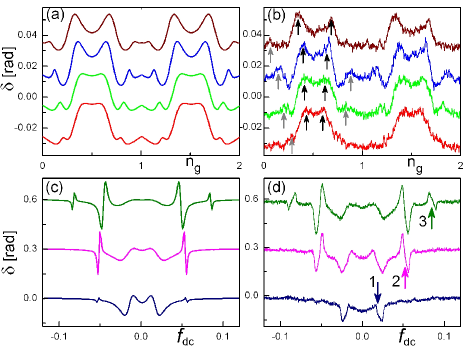
Figure 5: (Color online) Resonant excitation of the charge qubit probed by the tank circuit. The phase shift $\delta$ of the tank circuit coupled to the charge qubit, calculated theoretically (left) and measured (right). Panels (a) and (b) show the dependence on the gate voltage, while in (c) and (d) the dependence on the flux is demonstrated. Black and gray arrows in (c) demonstrate the positions of 1- and 2-photon resonant transitions, and the arrows in (d) mark 1-, 2-, and 3-photon excitations. Shnyrkov06

Theoretical fitting of the experimental graphs, as for example shown in Fig. 5, allows for defining the qubit’s parameters, which is the multiphoton spectroscopy. The parameters found were the following: the Josephson energies for the two junctions $E_{\mathrm{J}1}/h\simeq 40$ GHz and $E_{\mathrm{J}2}/h\simeq 34.5$ GHz, the island’s Coulomb energy $E_{\mathrm{C}}/h\simeq 5$ GHz; the relaxation and decoherence rates $\Gamma_{\mathrm{relax}}/(E_{\mathrm{C}}/h)=0.03$ and $\Gamma_{\phi}/(E_{\mathrm{C}}/h)=0.05$, which correspond to the following relaxation and decoherence times: $T_{\mathrm{relax}}=\Gamma_{\mathrm{relax}}^{-1}\simeq 7$ ns and $T_{\phi}=\Gamma_{\phi}^{-1}\simeq 4$ ns.

Figure 5 also demonstrates how the position of the resonances depend on the driving frequency $\omega$ and how the multiphoton resonances appear with increasing the driving power $n_{\mathrm{ac}}$. Namely, first, in Fig. 5(a,b) the varied parameter is the frequency $\omega/2\pi$, which from the bottom to top curves is $6.5$, $7.1$, $8.1$, and $9.1$ GHz; the driving power is the same for all figures $n_{\mathrm{ac}}\simeq 0.3$ and the flux was fixed at $\delta=\pi$. And, second, in Fig. 5(c,d) the curves correspond to the varied parameter driving power: in experiment being power of excitation (from bottom to top: $-80$, $-60$, $-57$ dB) and in theory being amplitude $n_{\mathrm{ac}}$ (from bottom to top: $0.1$, $0.2$, $0.4$); the frequency there was fixed, $\omega/2\pi=7$ GHz.

IV.4 One- and multiphoton transitions in the flux qubit

As we have seen in Section 3, both the tank voltage phase shift $\delta$ and amplitude $v$ can be used to monitor the resonant excitation of a superconducting qubit. In Fig. 5 we demonstrated this with the observation of the phase shift $\delta$ of the tank circuit coupled to the charge qubit. Now we consider one- and multi-photon resonant excitations of a flux qubit, and the nonmonotonic dependence of the tank voltage amplitude $v$ will visualize the resonant transitions in the qubit.

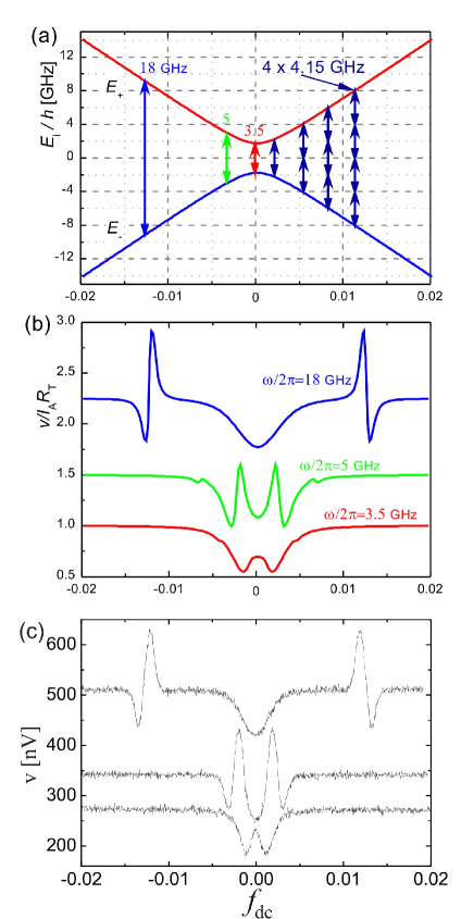
Figure 6: (Color online) Low-amplitude one-photon resonant excitation of a flux qubit. (a) Energy levels $E_{\pm}(f_{\mathrm{dc}})$ matched by the driving at frequencies shown by the numbers and the arrows of the respective length. (b) and (c) Theoretically calculated and experimentally measured amplitude of the tank voltage $v$ versus flux detuning $f_{\mathrm{dc}}$ for different driving frequencies. (The upper curves are shifted vertically.) The one-photon excitations at $\omega/2\pi=18$, $5$, and $3.5$ GHz, demonstrated in (b) and (c), are explained by the arrows to the left in the energy diagram (a), while the arrows to the right of the length $\omega/2\pi=4.15$ GHz explain the multiphoton resonances in Fig. 7. ShevchenkoPG08 ; Izmalkov08

Consider first the spectroscopical measurement, where the flux qubit is driven with the low-amplitude AC flux. We expect resonant excitation of the qubit when the driving frequency matches the qubit’s energy difference, $\hbar\omega=\Delta E(f_{\mathrm{dc}})$. In the experimental case the positions of these resonances at a given driving frequency allow to determine the energy structure of the measured qubit Izmalkov08 .

In Fig. 6(b,c) we demonstrate the dependence of the tank voltage amplitude $v$ on the bias flux $f_{\mathrm{dc}}$ at $\omega_{\mathrm{p}}=\omega_{0}$ for different driving frequencies: $\omega/2\pi=3.5,$ $5,$ and $18$ GHz, which is explained by the energy diagram in 6(a). The results of the related experiment, Ref. Izmalkov08 , are presented in Fig. 6(c). The parameters for calculations were taken as following: the tunneling amplitude $\Delta/h=3.5$ GHz, the energy bias $I_{\mathrm{p}}\Phi_{0}/h=700$ GHz, the temperature $k_{\mathrm{B}}T/h=1.4$ GHz, the relaxation rate $\Gamma_{1}/h=0.7$ GHz, the dephasing rate $\Gamma_{2}/h=0.7$ GHz, and the value which describes the coupling between the qubit and the tank circuit $k^{2}Q_{0}(LI_{\mathrm{p}}/\Phi_{0})=2.6\cdot 10^{-3}$. The curves were plotted for the driving amplitudes $f_{\mathrm{ac}}\cdot 10^{3}=1,$ $1.5,$ and $3$ from bottom to top. The phenomenological lagging parameter was taken $S=0.8$. Figure 6 demonstrates the effect described in section 3: for $S\neq 0$ both the phase shift $\delta$ and the amplitude $v$ depend on the qubit’s inductance $\mathcal{L}^{-1}$, which results in the alternation of peak and dip around the location of the resonances.

In Fig. 7(a,b) we present the calculated phase shift $\delta$ and the amplitude $v$ as functions of the probe current frequency $\omega_{\mathrm{p}}$ and the flux detuning $f_{\mathrm{dc}}$ with the phenomenological lagging parameter $S$ for the strongly-driven flux qubit with the parameters being the same as for Fig. 6 and with the values for the driving amplitude and frequency: $f_{\mathrm{ac}}=8\cdot 10^{-3}$ and $\omega/2\pi=4.15$ GHz. The top panel presents theoretical calculations, which is in good agreement with the experimental observations, presented in the bottom panel, Fig. 7(c,d). The dashed white line shows the tank resonance frequency $\omega_{\mathrm{p}}/2\pi=\omega_{0}/2\pi=20.8$ MHz. The positions of the multiphoton resonances is explained by the arrows to the right in the energy diagram, Fig. 6(a), at $\Delta E(f_{\mathrm{dc}})=k\hbar\omega$ with $k=1$, $2$, $3$, and $4$.

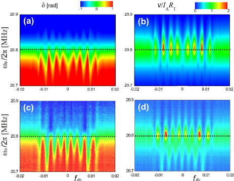
Figure 7: (Color online) Multiphoton excitations of a flux qubit. Theoretically calculated dependence of the phase shift $\delta$ (a) and the amplitude $v$ (b) on the bias current frequency $\omega_{\mathrm{p}}$ and the flux detuning $f_{\mathrm{dc}}$. (c,d) Experimentally measured phase shift $\delta$ and the amplitude $v$. ShevchenkoPG08

Note that for the lagging parameter close to $1$ (here $S=0.8$) the changes in the phase shift in Fig. 7(a) are small at the resonance frequency (along the dotted line at $\omega_{\mathrm{p}}=\omega_{0}$) while the voltage amplitude in Fig. 7(b) changes substantially, see formulas (39). And this is actually demonstrated in Fig. 6(b,c). Such changes of the tank effective resistance or, equivalently, quality factor were studied in Ref. Grajcar08 for the fully quantum-mechanical model of the qubit-resonator system. We note that this can be alternatively described with the semiclassical model, presented here. This model gives results consistent with the experimental ones, e.g. Figs. 6 and 7, which imply the energy transfer between the qubit and resonator according to Eq. (38). More details about this energy transfer, known as the Sisyphus damping and amplification, can be found in Refs. Grajcar08 , Skinner10 .

Then, in Fig. 8 we present the dependence of the tank voltage phase shift $\delta$ on the microwave amplitude $f_{\mathrm{ac}}$ and the DC flux bias $f_{\mathrm{dc}}$. This double quasi-periodical dependence (on both the energy bias and the driving amplitude) is called the Landau-Zener-Stückelberg interferogram Shevchenko10 . The parameters were taken the same as for Fig. 6 and $\omega/2\pi=4.15$ GHz. The left panel in Fig. 8 presents the theoretical interferogram from Ref. ShevchenkoPG08 while the right panel is the experimental one, Ref. Izmalkov08 . In Fig. 8 the multiphoton resonances at discrete DC bias $f_{\mathrm{dc}}$ (which controls the distance between energy levels) are clearly visible. These resonances appear when the energy of $k$ photons matches the qubit’s energy levels, $k\hbar\omega\approx\Delta E(f_{\mathrm{dc}})$. The quasi-periodical character of the dependence on the AC flux amplitude $f_{\mathrm{ac}}$ is known as Stückelberg oscillations. The comparison of such graph to the experimental analogue allows the relation of the microwave power to the AC flux amplitude $f_{\mathrm{ac}}$ to be determined, which is the calibration of the power. For this, either the estimation of the period of Stückelberg oscillations, shown by the black arrow, or adjusting the interference pattern slope, shown by the white line, can be used.

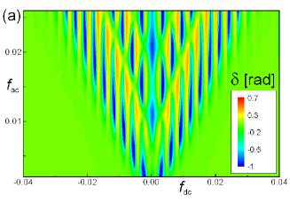
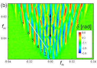
Figure 8: (Color online) LZS interferometry for the flux qubit probed by the tank circuit. The calculated (a) and measured (b) dependence of the tank phase shift on the flux detuning $f_{\mathrm{dc}}$ and on the driving flux amplitude $f_{\mathrm{ac}}$. ShevchenkoPG08 ; Izmalkov08

IV.5 Interferometry with nanoresonator

The formalism developed in Sec. 3.3 allows to describe the system of the driven qubit coupled to the NR. As it was demonstrated in Ref. Shevchenko11 , two different approaches, called direct and inverse LZS interferometry, are of interest. In the direct interferometry the qubit state is probed via the NR’s frequency shift, as in Ref. LaHaye09 , while in the inverse interferometry the impact of the NR’s state on the qubit’s Hamiltonian is studied.

The direct LZS interferometry was calculated in Ref. Shevchenko11 as the resonator’s frequency shift $\Delta\omega_{\mathrm{NR}}$ versus the energy bias $n_{\mathrm{g}}$ and the driving amplitude $n_{\mu}$. The agreement with the experimental result of Ref. LaHaye09 demonstrated that the semiclassical formalism is valid for a description of the measurable quantities. In Ref. Shevchenko11 it is also demonstrated how the analogous interferogram can be calculated for the qubit-tank circuit system in relation to the experiment of Ref. Sillanpaa06 . Such a description allows to correctly find the position of the resonance peaks in the interferogram and to demonstrate the sign-changing behaviour of the parametric capacitance, which relates to the measurable quantities.

For the formulation of the inverse problem, let us consider the qubit’s bias $\varepsilon_{0}$ as a function of the NR’s displacement $x$. For small $x\ll\xi$ we have the expansion (40), which results in the decomposition of the bias $\varepsilon_{0}(x)\approx\varepsilon_{0}^{\ast}(n_{\mathrm{g}})+\delta\varepsilon_{0}(x)$, where $\varepsilon_{0}^{\ast}(n_{\mathrm{g}})=8E_{\mathrm{C}}\left(n_{\mathrm{g}}-1/2\right)$ and $\delta\varepsilon_{0}(x)=8E_{\mathrm{C}}n_{\mathrm{NR}}x/\xi$. The Hamiltonian of the qubit (13) with the parameter-dependent bias $\varepsilon_{0}(x)$ allows to consider the following problem. Let us assume that the qubit’s state (its wave function, upper level occupation probability, Rabi frequency, etc.) is known (i.e. this is measured by a device, which we do not consider here for simplicity). Given the known qubit’s state, the aim is to find the Hamiltonian’s parameters. Particularly interesting is the parameter-dependent bias $\varepsilon_{0}(x)$, which can give the information about the position and amplitude of the oscillations of the NR.

And now, in the general context, the “reverse engineering” problem in the spirit of Refs. [Garanin02, ; Berry09, ] can be studied, where one is interested in finding the driving Hamiltonian for a given (desired) final state. On the other hand, in Ref. Shevchenko11 the authors provide the basis for measuring the NR’s position $x$ by means of probing the qubit’s state, while $x=x(t)$ is considered a slow time-dependent function. There, the emphasis was made on finding optimal driving and controlled offset ($\varepsilon_{0}^{\ast}$) parameters for the resolution of the small bias component $\delta\varepsilon_{0}$. It was assumed that the dynamics of the parameter $x$ is slow enough not to be considered during either certain period of the qubit’s evolution or even during the setting the stationary qubit’s state. The aim was to find a sensitive probe for small $\delta\varepsilon_{0}$. As the ultimate sensitivity, the essential changes of the qubit’s state for small changes of $\delta\varepsilon_{0}$ were required. The problem, formulated in this way, was solved in Ref. Shevchenko11 for different illustrative driving regimes: one-, double-, and multiple-passage regimes.

V 5. Multi-qubit systems

V.1 Equations for a system of coupled qubits

The effective Hamiltonian of the system of $n$ coupled flux qubits is

$$H=\sum\limits_{i=1}\left(-\frac{\Delta_{i}}{2}\sigma_{x}^{(i)}-\frac{\varepsilon_{i}(t)}{2}\sigma_{z}^{(i)}\right)+\sum\limits_{i,j}\frac{J_{ij}}{2}\sigma_{z}^{(i)}\sigma_{z}^{(j)},$$ (52)

where $J_{ij}$ is the coupling energy between qubits, and $\sigma_{x}^{(i)}$, $\sigma_{z}^{(i)}$ are the Pauli matrices in the basis $\{\left|\downarrow\right\rangle,\left|\uparrow\right\rangle\}$ of the current operator in the $i$-th qubit. The current operator is given by: $I_{i}=-I_{\mathrm{p}}^{(i)}\sigma_{z}^{(i)},$ with $I_{\mathrm{p}}^{(i)}$ the absolute value of the persistent current in the $i$-th qubit; then the eigenstates of $\sigma_{z}$ correspond to the clockwise ($\sigma_{z}\left|\downarrow\right\rangle=-\left|\downarrow\right\rangle$) and counterclockwise ($\sigma_{z}\left|\uparrow\right\rangle=\left|\uparrow\right\rangle$) current in the $i$-th qubit. The tunneling amplitudes $\Delta_{i}$ are assumed to be constants. The biases $\varepsilon_{i}=2I_{\mathrm{p}}^{(i)}\Phi_{0}f^{(i)}(t)$ are controlled by the dimensionless magnetic fluxes $f^{(i)}(t)=\Phi_{i}/\Phi_{0}-1/2$ through $i$-th qubit. These fluxes consist of three components,

$$f^{(i)}(t)=f_{i}+\frac{M_{i}I_{\mathrm{L}}}{\Phi_{0}}+f_{\mathrm{ac}}\sin\omega t.$$ (53)

Here $f_{i}$ is the adiabatically changing magnetic flux, experimentally applied by the coil and additional DC lines. The second term describes the flux induced by the current $I_{\mathrm{L}}$ in the tank coil, to which the $i$-th qubit is coupled with the mutual inductance $M_{i}$. And $f_{\mathrm{ac}}\sin\omega t$ is the harmonic time-dependent component driving the qubit, typically applied by an on-chip microwave antenna. Equation (52) can be reduced to the two-qubit system. This system is shown in Fig. 9.

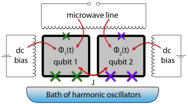
Figure 9: (Color online) Scheme of two coupled qubits. The two flux qubits are coupled to each other, to the dc and $\mu$w lines, as well as to an unavoidable dissipative environment. The convenient model for description of the environment is the bath of harmonic oscillators. The system of two coupled qubits is also assumed to be coupled to the measuring resonant circuit (which is not shown here), as in Fig. 2. Temchenko11

To describe the two-qubit system, it is convenient to present the density matrix in the following form

$$\rho = \frac{R_{\alpha\beta}}{4}\sigma_{\alpha}\otimes\sigma_{\beta}=\frac{R_{00}}{4}\sigma_{0}\otimes\sigma_{0}+$$

$$+\frac{R_{a0}}{4}\sigma_{a}\otimes\sigma_{0} + \frac{R_{0b}}{4}\sigma_{0}\otimes\sigma_{b}+\frac{R_{ab}}{4}\sigma_{a}\otimes\sigma_{b},$$ (54)

which was shown to be suitable for both the definition and the calculation of the entanglement and other characteristics in multi-qubit system, e.g. Schlienz95 ; Ivanchenko07 . Here $\alpha,\beta=0,x,y,z$ and $a,b=x,y,z$; the summation over twice repeating indices is assumed. The two vectors $R_{a0}$ and $R_{0b}$, so-called coherence vectors or Bloch vectors, determine the properties of the individual qubits, while the tensor $R_{ab}$ (the correlation tensor) accounts for the correlations.

The important characteristic of the state of the coupled-qubits system is its entanglement. There are different approaches to the quantification of the entanglement Love07 . One of the often used possibilities is the so-called concurrence Li08 . Another convenient for calculations approach is to introduce the measure of entanglement as following Schlienz95

$$\mathcal{E}=\frac{1}{3}\mathrm{Tr}\left(M^{T}M\right),\text{ }M_{ab}=R_{ab}-R_{a0}R_{0b}.$$ (55)

This entanglement measure fulfills certain requirements, in particular, $\mathcal{E}=0$ for any product state and $\mathcal{E}=1$ for any pure state with vanishing Bloch vectors $R_{a0}$ and $R_{0b}$, corresponding to maximum entangled states.

To describe dynamics of the density matrix we will first disregard the relaxation processes. This can be described by the Liouville equation, $i\hbar\dot{\rho}=\left[H,\rho\right]$, which is generally speaking a complex equation. To deal with the Liouville equation, it is convenient to use the parametrization of the density matrix as described by Eq. (54). Due to the hermiticity and normalization of the density matrix, $R_{\alpha\beta}$ are real numbers and $R_{00}=1$. Then the Liouville equation can be written in the form of the system of $15$ equations for $R_{\alpha\beta}$ Temchenko11

$$\dot{R}_{i0} = \epsilon_{mni}B_{m}^{(1)}R_{n0}+\epsilon_{3ni}JR_{n3},$$

$$\dot{R}_{0j} = \epsilon_{mnj}B_{m}^{(2)}R_{0n}+\epsilon_{3nj}JR_{3n},$$

$$\dot{R}_{ij} = \epsilon_{mni}B_{m}^{(1)}R_{nj}+\epsilon_{mnj}B_{m}^{(2)}R_{in}$$ (56)

$$+ \delta_{j3}\epsilon_{3ni}JR_{n0}+\delta_{i3}\epsilon_{3nj}JR_{0n},$$

where $\mathbf{B}^{(i)}=\left(-\Delta_{i},0,-\varepsilon_{i}\right)$ and $\epsilon_{mni}$ is the Levi-Civita symbol.

Consider now the measurable value, which is the resonator’s phase shift. As we discussed in Sec. 2, it relates to the effective inductance of qubits system. The formula obtained for single qubits can be generalized for the two-qubit system Grajcar05 ; Shevchenko08 . Then for the case of low-quality qubits, when their characteristic times are smaller than the tank’s period, at the resonance frequency ($\xi_{0}=0$), expression for the phase shift $\delta$ in terms of the parametric inductances $L_{\mathrm{q}}^{(i)}$ can be written as following

$$\tan\delta \approx Q_{0}\sum_{i=1,2}\frac{L_{0}}{L_{\mathrm{q}}^{(i)}},\text{ }$$ (57)

$$\frac{L_{0}}{L_{\mathrm{q}}^{(i)}} = k^{2}\frac{L_{i}}{\mathcal{L}_{i}}\text{ },\text{ }\mathcal{L}_{i}^{-1}=\left(\frac{\partial}{\partial\Phi_{a}}+\frac{\partial}{\partial\Phi_{b}}\right)I_{\mathrm{qb}}^{(i)}.$$

In what follows this expression will be used to calculate the phase shift $\delta$, which maps the qubits’ state.

V.2 Weak-driving spectroscopy

In Sec. 4 we have considered how the measurements of the single qubits allow to determine their parameters: the tunneling amplitudes $\Delta\$and the persistent currents $I_{\mathrm{p}}$. It was demonstrated Izmalkov08 that for defining the parameters of single and multiple-qubits systems both the ground-state measurements and excited-state spectroscopy can be used; the consistency of the results of the two approaches was shown. Now we will demonstrate this for the case of the system of two coupled flux qubits described by the Hamiltonian (52).

First, the one-qubit parameters are defined. For this, suppose qubit $a$ is the one biased far from its degeneracy point in such a way that $\varepsilon_{a}$ is large in comparison with the other energy variables. Then, qubit $a$ has a well defined ground state with averaged spin variables $\left\langle\sigma_{z}^{(a)}\right\rangle=1$ and $\left\langle\sigma_{x}^{(a)}\right\rangle=0$ which can be averaged out of the two-qubit Hamiltonian (52) reducing it to: $H_{\mathrm{2qbs,red}}=-\Delta_{b}\sigma_{x}^{(b)}/2-(\varepsilon_{b}-J)\sigma_{z}^{(b)}/2$. Apart from the offset in the bias term due to the coupling, this is identical to the single qubit Hamiltonian. This offset can be easily compensated and measured allowing the determination of the coupling energy $J$ Grajcar05 . The qubit parameters, $\Delta_{b}$ and $I_{\mathrm{p}}^{(b)}$, are determined from either the ground-state measurement or the excited-state spectroscopy, as it is described in Sec. 4. Analogously, biasing qubit $b$ far from the degeneracy point the parameters for qubit $a$, $\Delta_{a}$ and $I_{\mathrm{p}}^{(a)}$, can be determined. Next, the coupling energy $J$ was determined from the offset of the qubit dips from the $\Phi_{a/b}=0$ lines, visible in the pure ground-state measurements presented in Fig. 10(a).

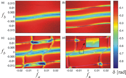
Figure 10: (Color online) Spectroscopy of the two-qubit system. The measured dependence of the phase shift $\delta$ on the flux biases $f_{a}$ and $f_{b}$: (a) ground-state measurement (without microwave excitation). (b,c,d) with weak microwave excitation at the driving frequencies $\omega/2\pi=$ $14.1$, $17.6$ and $20.7$ GHz. Izmalkov08

Then the qubits were driven by magnetic fluxes $\Phi_{\mathrm{ac}}\sin\omega t$ with weak driving amplitudes and various driving frequencies. There, we expect the position of the resonant transitions from energy level $E_{j}$ to an overlying level $E_{i}$ determined by the one-photon relation: $\Delta E_{ij}(\Phi_{a},\Phi_{b})\approx\hbar\omega$, which appears when the distance between the energy levels $\Delta E_{ij}=E_{i}-E_{j}$ is matched by the photon energy $\hbar\omega$. In Fig. 10(b) a frequency in-between both qubit gaps ($\Delta_{b}<\hbar\omega<\Delta_{a}$) was used and therefore only the transitions to the first excited state are visible. For higher frequencies, also the second and third excited states become visible as can be seen in subfigures (c) and (d). The theoretically calculated contour lines are superposed in Fig.  10(b-d) for three different frequencies for which the condition, $\Delta E_{ij}(\Phi_{a},\Phi_{b})=\hbar\omega$, is fulfilled; the energy levels $E_{i}=E_{i}(\Phi_{a},\Phi_{b})$ were found by diagonilizing the Hamiltonian. From the fitting procedure the following parameters were found: the tunneling amplitudes $\Delta_{a(b)}/h=15.8(3.5)$ GHz, the energy biases $I_{\mathrm{p}}^{a(b)}\Phi_{0}/h=375(700)$ GHz [$I_{\mathrm{p}}^{a(b)}=120(225)$ nA], the inter-qubit coupling $J/h=3.8$ GHz, and the value which describes the coupling between the qubits and the tank circuit $\Xi_{a(b)}=1.4(2.6)\cdot 10^{-3}$, where $\Xi_{i}=k_{i}^{2}Q_{0}(L_{i}I_{\mathrm{p}}^{(i)}/\Phi_{0})$.

V.3 Direct and ladder-type multiphoton transitions

We now consider the multiphoton excitations of a system of two strongly driven coupled flux qubits. We will describe the effects of resonant excitation in the system in terms of its energy structure, entanglement measure, and the observable tank circuit phase shift. Then we will present results for the multiphoton excitation of two types: direct (when multiple photon energy $k\hbar\omega$ matches the energy level difference $\Delta E_{ij}$) and ladder-type (when the transition happens via an intermediate level). We will demonstrate how this can be used for creating the inverse population in the dissipative two-qubit system.

To describe the system of two qubits subjected to the strong driving, the following values were calculated: the energy levels (by diagonalizing the stationary Hamiltonian), the density matrix $\rho$ (by solving the Liouville equation), the observable tank circuit phase shift $\delta$ (which is defined with the effective inductance of the qubits), and the entanglement measure $\mathcal{E}$ by making use of Eqs. (55-57). In this way graphs in Fig. 11 were calculated for the set of parameters of the two-qubit system realized in Ref. Izmalkov04a : $\Delta_{a}/h=1.2$ GHz, $\Delta_{b}/h=0.9$ GHz, $I_{\mathrm{p}}^{(a,b)}\Phi_{0}/h=$ $990$ GHz, $J/h=0.84$ GHz, $\Xi_{a,b}=1.8\cdot 10^{-3}$, and the driving frequency was taken $\omega/2\pi=4$ GHz; also the change of the DC flux here was assumed symmetrical: $f_{a}=f_{b}\equiv f_{\mathrm{dc}}$. For simplicity here the relaxation processes were ignored (and we will pay special attention to this below) and we consider the case when the characteristic measurement time $T_{\mathrm{p}}=2\pi/\omega_{\mathrm{p}}$ is larger than the characteristic times of the dynamics of the qubit. Then the tank circuit actually probes the incoherent mixture of qubit’s states and the time-averaged values of phase shift and entanglement should be considered.

When the energy of $k$ photons ($k\hbar\omega$) matches the energy difference between any two levels $E_{j}$ and $E_{i}$, the resonant excitation to the upper level is expected. Respectively, the arrows of the length $4$, $8$, and $12$ GHz show the places of possible one-, two-, and three-photon excitations. The time-averaged total probability of the currents in two qubits to flow clockwise, $Z=R_{03}+R_{30}$, is shown in Fig. 11(b) to experience resonant excitation. The resonances appear as peak-and-dip structures in the phase shift dependence in Fig. 11(c). The time-averaged entanglement measure $\mathcal{E}$ in a resonance increases due to the formation of the superposition of states, Fig. 11(d); this provides a method to control and probe the entanglement.

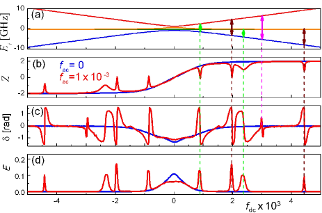
Figure 11: (Color online) Characterizing strongly-driven two-qubit system. Calculated and plotted as functions of the bias $f_{\mathrm{dc}}$ are four energy levels (a), total probability of the currents in two qubits to flow clockwise $Z$ (b), the tank circuit voltage phase shift $\delta$ (c), the entanglement measure $\mathcal{E}$ (d). ShevchenkoPG08

The experimental study of the strongly driven system of two coupled flux qubits is presented in Fig. 12. The left panel is the measured voltage amplitude of the tank as a function of qubit biases $f_{\mathrm{a}}$ and $f_{\mathrm{b}}$. The driving frequencies from top to bottom were $\omega/2\pi=17.6$, $7.0$, and $4.1$ GHz. The multiphoton resonances at $\Delta E_{ij}(f_{a},f_{b})\approx k\hbar\omega$ are visualized with the ridge-trough lines. We note that the resonance ridge-trough lines are disturbed with increasing or decreasing the signal; some of these changes are shown with white circles. This means changing the effective Josephson inductance in these points. The experimental results can be clearly understood by comparing them with the energy contour lines, calculated by diagonalizing Hamiltonian (52) and presented in the right panel of the figure. There, numbers $k-j$ next to the lines mean that the line relates to the energy difference $E_{j}-E_{k}$.

Consider now these multiphoton features in more details. In Fig. 12(b) the black and red lines show the positions of the expected resonant excitations from the ground state to the first and to the second excited states respectively; the blue and orange lines are the contour lines for the possible excitations from the first and from the second excited state to the third excited state. In Fig. 13(a) the energy levels are plotted at the fixed value of the bias flux through qubit $a$, $f_{\mathrm{a}}$, as a function of the bias flux through qubit $b$, $f_{\mathrm{b}}$. The arrows are introduced to match the energy levels with the driving frequencies $\omega/2\pi=17.6$ GHz and $7.0$ GHz . The black and red arrows in both Fig. 13(a) and Fig. 12(b) show the position of one-photon transitions to the first and the second excited levels. The double green and blue arrows in Fig. 12 show the position of the two-photon processes, where the excitation by the first photon creates the population of the first and the second levels and the second photon excites the system to the upper level. These two-photon excitations happen via intermediate levels; compare the position of these expected resonances in Fig. 12(b) shown with the blue circle and green square. The orange triangle in Fig. 12(b) points the ladder-type three-photon excitation, with one photon to the first excited level and then with two photons to the upper level.

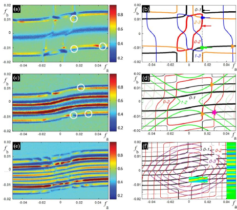
Figure 12: (Color online) Imaging the multiphoton transitions in the two-qubit system. The resonant excitation of the qubits system is visualized by the tank voltage amplitude, (a, c, e). The position of the resonant transitions can be understood by comparing with the respective energy contour lines (b, d, f). Ilichev10

Analogous considerations allow to see in Fig. 12(c) and (d) one- and two-photon resonant excitations to the first excited level for the driving frequency $\omega/2\pi=7$ GHz. The two-photon resonant excitation is direct and happen without any intermediate level. The higher level excitations via the first excited state appear due to three- and four-photon excitations, as shown with orange triangles and pink asterisk. In Fig. 12(e) the response of the two-qubit system at $\omega/2\pi=4.1$ GHz exhibits 1- to 4-photon excitations to the first excited state, which can be recognized by comparing with the black lines in Fig. 12(f). Numerous upper level excitations via the first excited level appear as the changes of the signal along these lines.

The transition rates can be quantified by the absolute value of the matrix element of the perturbation between the states $\left|E_{m}\right\rangle$ and $\left|E_{n}\right\rangle$

$$T_{nm}=\left|\left\langle E_{n}\right|\widehat{v}\left|E_{m}\right\rangle\right|^{2},\text{ \ }\widehat{v}=\frac{1}{I_{\mathrm{p}}^{(\mathrm{b})}}\left(I_{\mathrm{p}}^{(\mathrm{a})}\widehat{\sigma}_{z}^{(\mathrm{a})}+I_{\mathrm{p}}^{(\mathrm{b})}\widehat{\sigma}_{z}^{(\mathrm{b})}\right),$$ (58)

divided by the factor $I_{\mathrm{p}}^{(\mathrm{b})}\Phi_{0}f_{\mathrm{ac}}$. The transition matrix elements in Fig. 13(b) explain the ladder-type excitations in Fig. 12(b). Two points, marked by the vertical dashed green and blue lines in Fig. 13 describe respectively two interesting situations. To the right (see along the blue line) the transition element between the higher two levels ($E_{2}$ and $E_{3}$) is smaller than between the lower two levels ($E_{0}$ and $E_{2}$), $T_{02}\gg T_{23}\gg T_{03}$. In contrast, to the left (see along the green line) the transition element between the higher two levels ($E_{1}$ and $E_{3}$) is larger than between the lower two levels ($E_{0}$ and $E_{1}$), $T_{13}\gg T_{01}\gg T_{03}$. In both cases the probability of the direct excitation to the highest level is very small, which means that the transitions are induced due to the ladder-type mechanism.

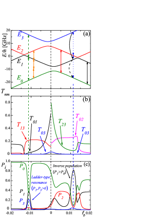
Figure 13: (Color online) Ladder-type transitions in the two-qubit system. Calculated as functions of the flux $f_{\mathrm{b}}$ (at $f_{\mathrm{a}}=0.015$): the energy levels (a), transition matrix elements $T_{nm}$ (b), the occupation probabilities $P_{i}$ (c). Ilichev10

The ladder-type transitions and the population inversion can be also illustrated by calculating the energy level occupation probabilities by solving the Bloch-Redfield equation (see the next subsection for more details); figure 13(c) was calculated with the driving frequency $\omega/2\pi=17.6$ GHz and amplitude $f_{\mathrm{ac}}=4\times 10^{-3}$. First, the ladder-type resonant excitation takes place to the left, where the upper level occupation probability $P_{3}$ is of the same order as the intermediate level occupation probability $P_{1}$. Second, the inverse population appears to the right, where the upper level occupation probability $P_{1}$ is larger than the ground state probability $P_{0}$, see also Refs. Astafiev07 ; You07 ; Berns08 ; Sun09 for the study of the population inversion in the systems with single Josephson-junction qubits. These two phenomena are similar to those which exhibit atoms in the laser field Vitanov01 . Furthermore, the expectation value of the current in $i$-th qubit is calculated with the reduced density matrix: $I_{\mathrm{qb}}^{(i)}=-I_{\mathrm{p}}^{(i)}Sp(\rho\sigma_{z}^{(i)})$. The results of the calculations are also presented as the color insets in Fig. 12(f) for the following parameters: the strength of dissipation $\alpha=0.1$ and the driving amplitude $f_{\mathrm{ac}}=8\times 10^{-3}$.

V.4 Lasing in the two-qubit system

Consider now the influence of the dissipation on the dynamics of a two-qubit system. For this the Bloch-Redfield formalism will be used. The strong dependence of the inter-level relaxation rates on the controlling magnetic fluxes will be demonstrated for the realistic system. This allows to propose several mechanisms for lasing in this four-level system Temchenko11 .

For identification of the level structure and understanding different transition rates it is instructive to start from considering the case of two non-interacting qubits, that is $J=0$. In this simplified situation, the energy levels of the system of two qubits consist of the pair-wise summation of single-qubit levels,

$$E_{i}^{\pm}=\pm\frac{\Delta E_{i}}{2}=\pm\frac{1}{2}\sqrt{\varepsilon_{i}^{(0)2}+\Delta_{i}^{2}}.$$ (59)

In Fig. 14(a) the energy levels are plotted as a function of the partial bias in the second qubit $f_{b}$, fixing the bias in the first qubit $f_{a}$. Then the single-qubit energy levels appear as the horizontal lines at $E_{a}^{\pm}=\pm\frac{1}{2}\sqrt{\varepsilon_{a}^{(0)2}+\Delta_{a}^{2}}$ and as the parabolas at $E_{b}^{\pm}(f_{b})=\pm\frac{1}{2}\sqrt{\varepsilon_{b}^{(0)}(f_{b})^{2}+\Delta_{b}^{2}}$. For the lasing the hierarchy of the relaxation times is required. For this it is natural to assume that the relaxation in the first qubit is much faster than in the second qubit. This allows to consider three- and four-level lasing schemes in Fig. 14(b,c).

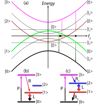
Figure 14: (Color online) Energy level structure with $J=0$. (a) One-qubit and two-qubit energy levels as functions of the magnetic flux $f_{b}$ at fixed flux $f_{a}$. The arrows show the fastest relaxation, which is assumed to relate to the qubit $a$. (b) and (c) Schemes for three- and four-level lasing at $f_{b}=f_{b\mathrm{L}}$ and $f_{b}=f_{b\mathrm{R}}$. The driving magnetic flux pumps (P) the upper level; fast relaxation (R) creates the population inversion; the two operating levels can be used for lasing (L). Temchenko11

As a next step, the interaction of the qubits, $J\neq 0$, should be considered. To describe the relaxation in this system, the operators are converted to the basis of eigenstates of the unperturbed Hamiltonian. In this representation $H_{0}^{\prime}=S^{-1}H_{0}S$ is the diagonal matrix; the unitary matrix $S$ consists of eigenvectors of the unperturbed Hamiltonian; the excitation operator $V(t)$ is converted as following

$$V^{\prime}(t)=S^{-1}V(t)S=\sum_{i=1,2}-\frac{1}{2}\widetilde{\varepsilon}_{i}(t)\tau_{z}^{(i)},\text{ }\tau_{z}^{(i)}=S^{-1}\sigma_{z}^{(i)}S.$$ (60)

The dissipative environment can be described as the thermostat, for which the convenient model is the bath of harmonic oscillators, see Fig. 9. Within the Bloch-Redfield formalism, the Liouville equation for the quantum system interacting with the bath is transformed into the master equation for the reduced system’s density matrix $\rho(t)$. Then the master equation for the density matrix of our driven system can be written in the energy representation as following Blum ; Weiss

$$\dot{\rho}_{ij}=-i\omega_{ij}\rho_{ij}-\frac{i}{\hbar}\left[V^{\prime},\rho\right]_{ij}+\delta_{ij}\sum_{n\neq j}\rho_{nn}W_{jn}-\gamma_{ij}\rho_{ij},$$ (61)

where $\omega_{ij}=(E_{i}-E_{j})/\hbar$, and the relaxation rates $W_{mn}=2$Re$\Gamma_{nmmn}$ and

$$\gamma_{mn}=\sum_{r}\left(\Gamma_{mrrm}+\Gamma_{nrrn}^{\ast}\right)-\Gamma_{nnmm}-\Gamma_{mmnn}^{\ast}$$ (62)

are defined by the relaxation tensor $\Gamma_{lmnk}$, which is given by the Fermi Golden rule. As it was shown in Refs. Governale01 ; Storcz03 ; vanderWal03 , the noise from the electromagnetic circuitry can be described in terms of the impedance $Z(\omega)$ from a bath of $LC$ oscillators, described by the Hamiltonian of interaction $H_{\mathrm{I}}=\frac{1}{2}\left(\sigma_{z}^{(a)}+\sigma_{z}^{(b)}\right)X$ in terms of the collective bath coordinate $X=\sum\nolimits_{k}c_{k}\Phi_{k}$. Here $\Phi_{k}$ stands for the magnetic flux in the $k$-th oscillator, which is coupled with the strength $c_{k}$ to the qubits. It follows that the relaxation tensor $\Gamma_{lmnk}$ is defined by the noise correlation function $S(\omega)$

$$\Gamma_{lmnk} = \frac{\Lambda_{lmnk}}{\hbar^{2}}S(\omega_{nk}),\text{ \ }S(\omega)=\int\limits_{0}^{\infty}dte^{-i\omega t}\left\langle X(t)X(0)\right\rangle,$$

$$\Lambda_{lmnk} = \left(\tau_{z}^{(1)}+\tau_{z}^{(2)}\right)_{lm}\left(\tau_{z}^{(1)}+\tau_{z}^{(2)}\right)_{nk}.$$ (63)

The correlator $S(\omega)$ was calculated in Refs. Governale01 ; Storcz03 within the spin-boson model and it was shown that the relevant real part of the relaxation tensor

$$\text{Re}\Gamma_{lmnk}=\frac{1}{8\hbar}\Lambda_{lmnk}J(\omega_{nk})\left[\coth\frac{\hbar\omega_{nk}}{2k_{B}T}-1\right]$$ (64)

is defined by the environmental Ohmic spectral density $J(\omega)=\alpha\hbar\omega$ and is cut off at some large value $\omega_{\mathrm{c}}$, where $\alpha$ is a parameter that describes the strength of the dissipative effects.

From the above equations the expression for the relaxation rates from level $\left|n\right\rangle$ to level $\left|m\right\rangle$ follows

$$W_{mn}=\frac{1}{4\hbar}\Lambda_{nmmn}J(\omega_{mn})\left[\coth\frac{\hbar\omega_{mn}}{2T}-1\right].$$ (65)

In Ref. Temchenko11 these relaxation rates were calculated as functions of the partial flux biases $f_{a}$ and $f_{b}$. It was demonstrated that the fastest transitions are those between the energy levels corresponding to changing the state of the first qubit and leaving the same state of the second qubit. Such a difference in the relaxation rates creates a sort of artificial selection rules for the transitions, similar to the selection rules studied e.g. in Refs. Liu05 ; deGroot10 ; Niemczyk11 . To describe the hierarchy of the relaxation rates, consider them in the simplified case, ignoring the interaction between the qubits; then the single-qubit relaxation rates follow from Eqs. (65) and (62) Blum ; Chirolli08

$$T_{1}^{-1} = W_{01}+W_{10}=\frac{\alpha\Delta^{2}}{2\hbar\Delta E}\coth\frac{\Delta E}{2T},$$ (66)

$$T_{2}^{-1} = \text{Re}\gamma_{01}=\frac{1}{2}T_{1}^{-1}+\frac{\alpha T}{\hbar}\frac{\varepsilon^{(0)2}}{\Delta E^{2}}.$$ (67)

In particular, in the vicinity of the point $f_{b}=f_{b}^{\ast}$ in Fig. 14(a), where $\Delta E^{(a)}=\Delta E^{(b)}$, we obtain $T_{1}^{(a)}/T_{1}^{(b)}\simeq\left(\Delta_{b}/\Delta_{a}\right)^{2}$. If $\Delta_{a}\gg\Delta_{b}$ is chosen, consequently the first qubit relaxes much faster.

After the parametrization of the density matrix, $\rho_{ij}=x_{ij}+iy_{ij}$, the system’s dynamics is described by the equations Temchenko11

$$\dot{x}_{ii}=-\frac{1}{\hbar}\left[V^{\prime},y\right]_{ii}+\sum_{r\neq i}W_{ir}x_{rr}-W_{ii}x_{ii},\text{ }i=1,2,3;$$ (68a)

$$\dot{x}_{ij}=\omega_{ij}y_{ij}-\frac{1}{\hbar}\left[V^{\prime},y\right]_{ij}-\gamma_{ij}x_{ij},\text{ }i>j;$$ (68b)

$$\dot{y}_{ij}=-\omega_{ij}x_{ij}+\frac{1}{\hbar}\left[V^{\prime},y\right]_{ij}-\gamma_{ij}y_{ij},\text{ }i>j;$$ (68c)

$$y_{ii}=0 x_{00}=1-(x_{11}+x_{22}+x_{33}) x_{ji}=x_{ij} y_{ji}=-y_{ij}$$, ; , .

When discussing Fig. 14 we pointed out that in the system of two coupled qubits there are two ways to realize lasing, making use of the three or four levels to create the population inversion between the operating levels. In Ref. Temchenko11 the lasing in the two-qubit system was demonstrated by solving numerically the Bloch-type equations (68). Besides demonstrating the population inversion between the operating levels, an additional signal with the frequency matching the distance between the operating levels was applied, to stimulate the transition from the upper operating level to the lower one. So, the driving was considered to be, first, the monochromatic signal $f(t)=f_{\mathrm{ac}}\sin\omega t$ to pump the system to the upper level and to demonstrate the population inversion. Then another signal stimulating transitions between the operating laser levels is applied $f(t)=f_{\mathrm{ac}}\sin\omega t+f_{\mathrm{L}}\sin\omega_{\mathrm{L}}t$ with $\hbar\omega_{\mathrm{L}}=E_{2}-E_{1}$. Solving the system of equations (68), one obtains the population of $i$-th level of our two-qubit system, $P_{i}=x_{ii}$. The results of the calculations are presented in Fig. 15, where the temporal dynamics of the level populations is given for two situations.

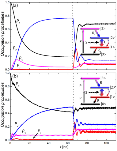
Figure 15: (Color online) Two-qubit lasing and stimulated transition. The time-dependent occupation probabilities are plotted for one- and two-photon driving. The driving and fast relaxation create the inverse population between the levels $\lvert{2}\rangle$ and $\lvert{1}\rangle$; then the stimulating signal $f_{\mathrm{L}}\cos\omega_{\mathrm{L}}t$ is turned on. Temchenko11

As shown in the inset schemes in Fig. 15, the fastest (dominating) relaxation transitions are $\lvert{3}\rangle\rightarrow\lvert{2}\rangle$ and $\lvert{1}\rangle\rightarrow\lvert{0}\rangle$. The system is excited by either one- or two-photon transitions, with $\hbar\omega=E_{3}-E_{0}$ in Fig. 15(a) or with $2\hbar\omega=E_{3}-E_{0}$ in Fig. 15(b). This creates the population inversion between the levels $\lvert{2}\rangle\$and $\lvert{1}\rangle$. Note that analogous competition of the driving and relaxation can lead to the population inversion in other multi-level systems Goorden05 ; Du10b . Fast relaxation, $\lvert{1}\rangle\rightarrow\lvert{0}\rangle$, helps creating the population inversion between the laser levels $\lvert{2}\rangle\$and $\lvert{1}\rangle$, which is the advantage of the four-level scheme Svelto . Then the transition $\lvert{2}\rangle\rightarrow\lvert{1}\rangle$ is stimulated by another signal with a frequency matching the laser operating levels ($\hbar\omega_{\mathrm{L}}=E_{2}-E_{1}$). Figure 15 was calculated for the following realistic parameters Ilichev10 : $\Delta_{a}/h=15.8$ GHz, $\Delta_{b}/h=3.5$ GHz, $I_{\mathrm{p}}^{(a)}\Phi_{0}/h=375$ GHz, $I_{\mathrm{p}}^{(b)}\Phi_{0}/h=700$ GHz, $J/h=3.8$ GHz, $k_{B}T/h=1$ GHz; and also $\omega_{\mathrm{L}}/2\pi=9$ GHz, $f_{\mathrm{L}}=f_{\mathrm{ac}}=5\times 10^{-3}$ with the driving frequency $\omega/2\pi=47.4$ GHz for (a) and $\omega/2\pi=23.7$ GHz for (b).

For the realization of such lasing schemes, the system of two qubits should be put in a quantum resonator, e.g. by coupling to a transmission line resonator, as in Ref. Astafiev07, . Then the stimulated transition between the operating states, demonstrated in Fig. 15, will result in transmitting the energy from the qubits to the resonator as photons.

VI Conclusions

Here we presented the experimental and theoretical results of the study of driven single and coupled superconducting qubits. The multiphoton transitions in both charge and flux qubits were studied in details. Those processes are important for both demonstrating the fundamental quantum phenomena in mesoscopic systems and for developing controlling mechanisms for perspective devices.

The system of qubits, coupled to the controlling electronics and measuring resonator, can be described within the semiclassical approach. After presenting this formalism in application to probing the qubit systems, we have shown some specific experimental results, which were accompanied by the calculated counterparts. The agreement between them shows contemporary possibility to demonstrate and describe quantum phenomena in mesoscopic systems.

- (1) C. Cohen-Tannoudji, J. Dupont-Roc, and G. Grynberg, Atom-Photon Interactions, Wiley, New York (1992).
- (2) N. B. Delone and V. P. Krainov, Atoms in Strong Light Fields, Springer Ser. Chem. Phys., Vol. 28, Springer, Berlin–Heidelberg (1985) [also in Russian: Atom v sil’nom svetovom pole, Atomizdat, Moscow (1978)].
- (3) C. Xu, W. Zipfel, J. B. Shear, R. M. Williams, and W. W. Webb, Proc. Natl. Acad. Sci. USA 93, 10763 (1996).
- (4) K. König, J. Microsc. 200, 83 (2000).
- (5) A. Diaspro, P. Bianchini, G. Vicidomini, M. Faretta, P. Ramoino, and C. Usai, BioMedical Engineering OnLine 5, 36 (2006).
- (6) Yu. Makhlin, G. Schön, and A. Shnirman, Rev. Mod. Phys. 73, 357 (2001).
- (7) M. H. Devoret and J. M. Martinis, Quantum Inf. Process. 3, 163 (2004).
- (8) G. Wendin and V.S. Shumeiko, arXiv:cond-mat/0508729; Low Temp. Phys. 33, 724 (2007).
- (9) J. Clarke and F. K. Wilhelm, Nature 453, 1031 (2008).
- (10) J. Q. You and F. Nori, Nature 474, 589 (2011).
- (11) Y. Nakamura, Yu. A. Pashkin, and J. S. Tsai, Nature 398, 786 (1999).
- (12) J. R. Friedman, V. Patel, W. Chen, S. K. Tolpygo, and J. E. Lukens, Nature 406, 43 (2000).
- (13) C. H. van der Wal, A. C. J. ter Haar, F. K. Wilhelm, R. N. Schouten, C. J. P. M. Harmans, T. P. Orlando, S. Lloyd, and J. E. Mooij, Science 290, 773 (2000).
- (14) D. Vion, A. Aassime, A. Cottet, P. Joyez, H. Pothier, C. Urbina, D. Esteve, and M. H. Devoret, Physica Scripta T102, 162 (2002).
- (15) Y. Yu, S. Han, X. Chu, S.-I Chu, and Z. Wang, Science 296, 889 (2002).
- (16) J. Martinis, S. Nam, J. Aumentado, and C. Urbina, Phys. Rev. Lett. 89, 117901 (2002).
- (17) I. Chiorescu, Y. Nakamura, C. J. P. M. Harmans, and J. E. Mooij, Science 299, 1869 (2003).
- (18) D. Born, V. I. Shnyrkov, W. Krech, Th. Wagner, E. Il’ichev, M. Grajcar, U. Hübner, and H.-G. Meyer, Phys. Rev. B 70, 180501(R) (2004).
- (19) J. Claudon, F. Balestro, F. W. J. Hekking, and O. Buisson, Phys. Rev. Lett. 93, 187003 (2004).
- (20) D. M. Berns, M. S. Rudner, S. O. Valenzuela, K. K. Berggren, W. D. Oliver, L. S. Levitov, and T. P. Orlando, Nature 455, 51 (2008).
- (21) M. Neeley, M. Ansmann, R. C. Bialczak, M. Hofheinz, E. Lucero, A. D. O’Connell, D. Sank, H. Wang, J. Wenner, A. N. Cleland, M. R. Geller, and J. M. Martinis, Science 325, 722 (2009).
- (22) F. Nori, Science 325, 689 (2009).
- (23) H. Jirari, F. W. J. Hekking, and O. Buisson, Europhys. Lett. 87, 28004 (2009).
- (24) M. A. Sillanpää, J. Sarkar, J. Sulkko, J. Muhonen, and P. J. Hakonen, Appl. Phys. Lett. 95, 011909 (2009).
- (25) J. Joo, J. Bourassa, A. Blais, and B. C. Sanders, Phys. Rev. Lett. 105, 073601 (2010).
- (26) L. Du and Y. Yu, Phys. Rev. B 82, 144524 (2010).
- (27) Y. Nakamura, Yu. A. Pashkin, and J. S. Tsai, Phys. Rev. Lett. 87, 246601 (2001).
- (28) A. Wallraff, T. Duty, A. Lukashenko, and A. V. Ustinov, Phys. Rev. Lett. 90, 037003 (2003).
- (29) S. Saito, M. Thorwart, H. Tanaka, M. Ueda, H. Nakano, K. Semba, and H. Takayanagi, Phys. Rev. Lett. 93, 037001 (2004).
- (30) V. I. Shnyrkov, Th. Wagner, D. Born, S. N. Shevchenko, W. Krech, A. N. Omelyanchouk, E. Il’ichev, and H.-G. Meyer, Phys. Rev. B 73, 024506 (2006).
- (31) V. I. Shnyrkov, D. Born, A. A. Soroka, and W. Krech, Phys. Rev. B 79, 184522 (2009).
- (32) Y. Yu, W. D. Oliver, J. C. Lee, K. K. Berggren, L. S. Levitov, and T. P. Orlando, arXiv:cond-mat/0508587.
- (33) F. W. Strauch, S. K. Dutta, H. Paik, T. A. Palomaki, K. Mitra, B. K. Cooper, R. M. Lewis, J. R. Anderson, A. J. Dragt, C. J. Lobb, and F. C. Wellstood, IEEE Trans. Appl. Supercond. 17, 105 (2007).
- (34) S. K. Dutta, F. W. Strauch, R. M. Lewis, K. Mitra, H. Paik, T. A. Palomaki, E. Tiesinga, J. R. Anderson, A. J. Dragt, C. J. Lobb, and F. C. Wellstood, Phys. Rev. B 78, 104510 (2008).
- (35) Y. Wang, S. Cong, X. Wen, C. Pan, G. Sun, J. Chen, L. Kang, W. Xu, Y. Yu, and P. Wu, Phys. Rev. B 81, 144505 (2010).
- (36) P. Bushev, C. Muller, J. Lisenfeld, J. H. Cole, A. Lukashenko, A. Shnirman, and A. V. Ustinov, Phys. Rev. B 82, 134530 (2010).
- (37) S. N. Shevchenko, S. Ashhab, and F. Nori, Phys. Rep. 492, 1 (2010).
- (38) W. D. Oliver, Y. Yu, J. C. Lee, K. K. Berggren, L. S. Levitov, and T. P. Orlando, Science 310, 1653 (2005).
- (39) M. Sillanpää, T. Lehtinen, A. Paila, Yu. Makhlin, and P. Hakonen, Phys. Rev. Lett. 96, 187002 (2006).
- (40) C. M. Wilson, T. Duty, F. Persson, M. Sandberg, G. Johansson, and P. Delsing, Phys. Rev. Lett. 98, 257003 (2007).
- (41) A. Izmalkov, S. H. W. van der Ploeg, S. N. Shevchenko, M. Grajcar, E. Il’ichev, U. Hübner, A. N. Omelyanchouk, and H.-G. Meyer, Phys. Rev. Lett. 101, 017003 (2008).
- (42) G. Sun, X. Wen, Y. Wang, S. Cong, J. Chen, L. Kang,W. Xu, Y. Yu, S. Han, and P. Wu, Appl. Phys. Lett. 94, 102502 (2009).
- (43) M. D. LaHaye, J. Suh, P. M. Echternach, K. C. Schwab, and M. L. Roukes, Nature 459, 960 (2009).
- (44) Yu. A. Pashkin, T. Yamamoto, O. Astafiev, Y. Nakamura, D. V. Averin, and J. S. Tsai, Nature 421, 823 (2003).
- (45) A. J. Berkley, H. Xu, R. C. Ramos, M. A. Gubrud, F. W. Strauch, P. R. Johnson, J. R. Anderson, A. J. Dragt, C. J. Lobb, and F. C. Wellstood, Science 300, 1548 (2003).
- (46) J. B. Majer, F. G. Paauw, A. C. J. ter Haar, C. J. P. M. Harmans, and J. E. Mooij, Phys. Rev. Lett. 94, 090501 (2005).
- (47) M. Steffen, M. Ansmann, R. C. Bialczak, N. Katz, E. Lucero, R. McDermott, M. Neeley, E. M. Weig, A. N. Cleland, and J. M. Martinis, Science 313, 423 (2006).
- (48) J. H. Plantenberg, P. C. de Groot, C. J. P. M. Harmans, and J.E. Mooij, Nature 447, 836 (2007).
- (49) A. Fay, E. Hoskinson, F. Lecocq, L. P. Levy, F. W. J. Hekking, W. Guichard, and O. Buisson, Phys. Rev. Lett. 100, 187003 (2008).
- (50) L. DiCarlo, J. M. Chow, J. M. Gambetta, L. S. Bishop, B. R. Johnson, D. I. Schuster, J. Majer, A. Blais, L. Frunzio, S. M. Girvin, and R. J. Schoelkopf, Nature 460, 240 (2009).
- (51) F. Altomare, J. I. Park, K. Cicak, M. A. Sillanpää, M. S. Allman, D. Li, A. Sirois, J. A. Strong, J. D. Whittaker, and R. W. Simmonds, Nature Phys. 6, 777 (2010).
- (52) P. J. Leek, S. Filipp, P. Maurer, M. Baur, R. Bianchetti, J.M. Fink, M. Göppl, L. Steffen, and A. Wallraff, Phys. Rev. B 79, 180511(R) (2009).
- (53) E. Il’ichev, S. N. Shevchenko, S. H. W. van der Ploeg, M. Grajcar, E. A. Temchenko, A. N. Omelyanchouk, and H.-G. Meyer, Phys. Rev. B 81, 012506 (2010).
- (54) E. A. Temchenko, S. N. Shevchenko, and A. N. Omelyanchouk, Phys. Rev. B 83, 144507 (2011).
- (55) A. M. Satanin, M. V. Denisenko, S. Ashhab, and F. Nori, arXiv:1201.1901.
- (56) T.-S. Ho, S.-H. Hung, H.-T. Chen, and S.-I Chu, Phys. Rev. B 79, 235323 (2009).
- (57) H. Ribeiro, J. R. Petta, and G. Burkard, Phys. Rev. A 82, 115445 (2010).
- (58) A. Brataas and E. I. Rashba, Phys. Rev. B 84, 045301 (2011).
- (59) Y. Dovzhenko, J. Stehlik, K. D. Petersson, J. R. Petta, H. Lu, and A. C. Gossard, Phys. Rev. B 84, 161302(R) (2011).
- (60) L. Gaudreau, G. Granger, A. Kam, G. C. Aers, S. A. Studenikin, P. Zawadzki, M. Pioro-Ladrière, Z. R. Wasilewski, and A. S. Sachrajda, Nature Phys. 8, 54 (2012).
- (61) L. Childress and J. McIntyre, Phys. Rev. A 82, 033839 (2010).
- (62) P. Huang, J. Zhou, F. Fang, X. Kong, X. Xu, C. Ju, and J. Du, Phys. Rev. X 1, 011003 (2011).
- (63) A. Zenesini, D. Ciampini, O. Morsch, and E. Arimondo, Phys. Rev. A 82, 065601 (2010).
- (64) P. Plötz and S. Wimberger, Eur. Phys. J. D 65, 199 (2011).
- (65) J.-N. Zhang, C.-P. Sun, S. Yi, and F. Nori, Phys. Rev. A 83, 033614 (2011).
- (66) G. Heinrich, J. G. E. Harris, and F. Marquardt, Phys. Rev. A 81, 011801(R) (2010).
- (67) L. Chotorlishvili, A. Ugulava, G. Mchedlishvili, A. Komnik, S. Wimberger, and J. Berakdar, J. Phys. B 44, 215402 (2011).
- (68) N. Miladinovic, F. Hasan, N. Chisholm, I. E. Linnington, E. A. Hinds, and D. H. J. O’Dell, Phys. Rev. A 84, 043822 (2011).
- (69) S. Bertaina, N. Groll, L. Chen, and I. Chiorescu, J. Phys.: Conf. Ser. 324, 012008 (2011).
- (70) A. T. Hatke, M. Khodas, M. A. Zudov, L. N. Pfeiffer, and K.W. West, Phys. Rev. B 84, 241302(R) (2011).
- (71) H. K. Avetissian, A. K. Avetissian, G. F. Mkrtchian, and Kh. V. Sedrakian, Phys. Rev. B 85, 115443 (2012).
- (72) V. B. Braginsky and F. Ya. Khalili, Quantum Measurement (Cambridge University Press, 1992).
- (73) E. Il’ichev, Th. Wagner, L. Fritzsch, J. Kunert, V. Schultze, T. May, H.E. Hoenig, H.-G. Meyer, M. Grajcar, D. Born, W. Krech, M. Fistul, and A. Zagoskin, Appl. Phys. Lett. 80, 4184, (2002).
- (74) E. Il’ichev, S. H. W. van der Ploeg, M. Grajcar, and H.-G. Meyer, Quantum Inf. Process. 8, 133 (2009).
- (75) E. K. Irish and K. C. Schwab, Phys. Rev. B 68, 155311 (2003).
- (76) A. Blais, R.-S. Huang, A. Wallraff, S. M. Girvin, and R. J. Schoelkopf, Phys. Rev. A 69, 062320 (2004).
- (77) D. I. Schuster, A. Wallraff, A. Blais, L. Frunzio, R.-S. Huang, J. Majer, S. M. Girvin, and R. J. Schoelkopf, Phys. Rev. Lett. 94, 123602 (2005).
- (78) A. A. Abdumalikov, Jr., O. Astafiev, Y. Nakamura, Yu. A. Pashkin, and J. S. Tsai, Phys. Rev. B 78, 180502(R) (2008).
- (79) G. Oelsner, S. H. W. van der Ploeg, P. Macha, U. Hübner, D. Born, S. Anders, E. Il’ichev, H.-G. Meyer, M. Grajcar, S. Wünsch, M. Siegel, A. N. Omelyanchouk, and O. Astafiev, Phys. Rev. B 81, 172505 (2010).
- (80) A. N. Omelyanchouk, S. N. Shevchenko, Ya. S. Greenberg, O. Astafiev and E. Il’ichev, Low Temp. Phys. 36, 893 (2010).
- (81) S. Ashhab and F. Nori, Phys. Rev. A 81, 042311 (2010).
- (82) T. Niemczyk, F. Deppe, H. Huebl, E. P. Menzel, F. Hocke, M. J. Schwarz, J. J. Garcia-Ripoll, D. Zueco, T. Hummer, E. Solano, A. Marx, and R. Gross, Nature Phys. 6, 772 (2010).
- (83) L. S. Bishop, J. M. Chow, J. Koch, A. A. Houck, M. H. Devoret, E. Thuneberg, S. M. Girvin, and R. J. Schoelkopf, Nature Phys. 5, 105 (2009).
- (84) T. Niemczyk, F. Deppe, M. Mariantoni, E. P. Menzel, E. Hoffmann, G. Wild, L. Eggenstein, A. Marx, and R. Gross, Supercond. Sci. Technol. 22, 034009 (2009).
- (85) J. M. Fink, M. Baur, R. Bianchetti, S. Filipp, M. Göppl1, P. J. Leek, L. Steffen, A. Blais, and A. Wallraff, Phys. Scr. T137, 014013 (2009).
- (86) J.-W. Pan, Z.-B. Chen, C.-Y. Lu, H. Weinfurter, A. Zeilinger, and M. Źukowski, arXiv:0805.2853; Rev. Mod. Phys., accepted.
- (87) S. N. Shevchenko, S. H. W. van der Ploeg, M. Grajcar, E. Il’ichev, A. N. Omelyanchouk, and H.-G. Meyer, Phys. Rev. B 78, 174527 (2008).
- (88) S. N. Shevchenko, S. Ashhab, and F. Nori, Phys. Rev. B 85, 094502 (2012).
- (89) N. N. Bogolyubov and Yu. A. Mitropol’skii, Asymptotic Methods in the Theory of Nonlinear Oscillations (Nauka, Moscow, 1974; Gordon and Breach, New York, 1962).
- (90) M. Grajcar, S. H. W. van der Ploeg, A. Izmalkov, E. Il’ichev, H.-G. Meyer, A. Fedorov, A. Shnirman, and G. Schön, Nature Phys. 4, 612 (2008).
- (91) R. Rifkin and B. S. Deaver, Jr., Phys. Rev. B 13, 3894 (1976).
- (92) Ya. S. Greenberg, A. Izmalkov, M. Grajcar, E. Il’ichev, W. Krech, and H.-G. Meyer, Phys. Rev. B 66, 224511 (2002).
- (93) A.Yu. Smirnov, Phys. Rev. B 68, 134514 (2003).
- (94) T. P. Orlando, J. E. Mooij, L. Tian, C. H. van der Wal, L. S. Levitov, S. Lloyd, and J. J. Mazo, Phys. Rev. B 60, 15399 (1999).
- (95) K. K. Likharev, Dynamics of Josephson Junctions and Circuits, Gordon Breach, Amsterdam (1986).
- (96) Ya. S. Greenberg and E. Il’ichev, Phys. Rev. B 77, 094513 (2008).
- (97) S. N. Shevchenko, Eur. Phys. J. B 61, 187 (2008).
- (98) Ya. S. Greenberg, A. Izmalkov, M. Grajcar, E. Il’ichev, W. Krech, H.-G. Meyer, M. H. S. Amin, and A. Maassen van den Brink, Phys. Rev. B 66, 214525 (2002).
- (99) M. A. Sillanpää, T. Lehtinen, A. Paila, Yu. Makhlin, L. Roschier, and P. J. Hakonen, Phys. Rev. Lett. 95, 206806 (2005).
- (100) T. Duty, G. Johansson, K. Bladh, D. Gunnarsson, C. Wilson, and P. Delsing, Phys. Rev. Lett. 95, 206807 (2005).
- (101) G. Johansson, L. Tornberg, V. S. Shumeiko and G. Wendin, Condens. Matter 18, S901 (2006).
- (102) K. Blum, Density Matrix Theory and Applications, Plenum Press, New York–London (1981).
- (103) U. Weiss, Quantum Dissipative Systems, 2nd ed., World Scientific, Singapore (1999).
- (104) F. H. M. Faisal, Theory of Multiphoton Processes, Plenum Press, New York (1987).
- (105) H. Nakamura, Nonadiabatic Transition: Concepts, Basic Theories, and Applications (2nd ed., World Scientific, Singapore, 2012).
- (106) M. Grifoni and P. Hänggi, Phys. Rep. 304, 229 (1998).
- (107) S.-I Chu and D. A. Telnov, Phys. Rep. 390, 1 (2004).
- (108) B. M. Garraway and N. V. Vitanov, Phys. Rev. A 55, 4418 (1997).
- (109) M. Førre, Phys. Rev. A 70, 013406 (2004).
- (110) S.-K. Son, S. Han, and S.-I Chu, Phys. Rev. B 79, 032301 (2009).
- (111) X. Wen and Y. Yu, Phys. Rev. B 79, 094529 (2009).
- (112) A. Ferrón, D. Domínguez, and M. J. Sánchez, Phys. Rev. B 82, 134522 (2010).
- (113) J. H. Shirley, Phys. Rev. 138, B979 (1965).
- (114) V. P. Krainov and V. P. Yakovlev, JETP 51, 1104 (1980).
- (115) J. Tuorila, M. Silveri, M. Sillanpää, E. Thuneberg, Yu. Makhlin, and P. Hakonen, Phys. Rev. Lett. 105, 257003 (2010).
- (116) J.-M. Lopez-Castillo, A. Filali-Mouhim, and J.-P. Jay-Gerin, J. Chem. Phys. 97, 1905 (1992).
- (117) S. Ashhab, J. R. Johansson, A. M. Zagoskin, and F. Nori, Phys. Rev. A 75, 063414 (2007).
- (118) I. Tornes and D. Stroud, Phys. Rev. B 77, 224513 (2008).
- (119) N. Grønbech-Jensen and M. Cirillo, Phys. Rev. Lett. 95, 067001 (2005).
- (120) J. E. Marchese, M. Cirillo, and N. Grønbech-Jensen, Open Systems and Information Dynamics 14, 189 (2007).
- (121) S. N. Shevchenko, A. N. Omelyanchouk, A. M. Zagoskin, S. Savel’ev, and F. Nori, New J. Phys. 10, 073026 (2008).
- (122) S. N. Shevchenko, A. S. Kiyko, A. N. Omelyanchouk, W. Krech, Low Temp. Phys. 31, 569 (2005).
- (123) A. J. Leggett, S. Chakravarty, A. T. Dorsey, M. P. A. Fisher, A. Garg, W. Zwerger, Rev. Mod. Phys. 59, 1 (1987).
- (124) M. C. Goorden, M. Thorwart, and M. Grifoni, Eur. Phys. J. B 45, 405 (2005).
- (125) A. P. Saiko, G. G. Fedoruk, and S. A. Markevich, JETP 105, 893 (2007).
- (126) S. Saito, T. Meno, M. Ueda, H. Tanaka, K. Semba, and H. Takayanagi, Phys. Rev. Lett. 96, 107001 (2006).
- (127) D. Gunnarsson, J. Tuorila, A. Paila, J. Sarkar, E. Thuneberg, Yu. Makhlin, and P. Hakonen, Phys. Rev. Lett. 101, 256806 (2008).
- (128) A. Paila, J. Tuorila, M. Sillanpää, D. Gunnarsson, J. Sarkar, Yu. Makhlin, E. Thuneberg, and P. Hakonen, Quantum Inf. Process. 8, 245 (2009).
- (129) Ya. S. Greenberg, E. Il’ichev, and A. Izmalkov, Europhys. Lett. 72, 880 (2005).
- (130) A. N. Omelyanchouk, S. Savel’ev, A. M. Zagoskin, E. Il’ichev, and F. Nori, Phys. Rev B 80, 212503 (2009).
- (131) W. Krech, M. Grajcar, D. Born, I. Zhilyaev, Th. Wagner, E. Il’ichev, and Ya. Greenberg, Phys. Lett. A 303, 352 (2002).
- (132) A. B. Zorin, Physica C 368, 284 (2002).
- (133) E. Il’ichev, A.Yu. Smirnov, M. Grajcar, A. Izmalkov, D. Born, N. Oukhanski, Th. Wagner, W. Krech, H.-G. Meyer, and A. Zagoskin, Low Temp. Phys. 30, 620 (2004).
- (134) M. Grajcar, A. Izmalkov, E. Il’ichev, Th. Wagner, N. Oukhanski, U. Hübner, T. May, I. Zhilyaev, H. E. Hoenig, Ya. S. Greenberg, V. I. Shnyrkov, D. Born, W. Krech, H.-G. Meyer, A. Maassen van den Brink, and M. H. S. Amin, Phys. Rev. B 69, 060501 (2004).
- (135) J. C. Skinner, H. Prance, P. B. Stiffell, and R. J. Prance, Phys. Rev. Lett. 105, 257002 (2010).
- (136) D. A. Garanin and R. Schilling, Europhys. Lett. 59, 7 (2002).
- (137) M. V. Berry, J. Phys. A: Math. Theor. 42, 365303 (2009).
- (138) J. Schlienz and G. Mahler, Phys. Rev. A 52, 4396 (1995).
- (139) E. A. Ivanchenko, Low Temp. Phys. 33, 336 (2007).
- (140) P. J. Love, A. Maassen van den Brink, A. Yu. Smirnov, M. H. S. Amin, M. Grajcar, E. Il’ichev, A. Izmalkov, and A. M. Zagoskin, Quantum Inf. Process. 6, 187 (2007).
- (141) J. Li, K. Chalapat, and G. S. Paraoanu, Phys. Rev. B 78, 064503 (2008).
- (142) M. Grajcar, A. Izmalkov, S. H. W. van der Ploeg, S. Linzen, E. Il’ichev, Th. Wagner, U. Hübner, H.-G. Meyer, A. Maassen van den Brink, S. Uchaikin, and A. M. Zagoskin, Phys. Rev. B 72, 020503(R) (2005).
- (143) A. Izmalkov, M. Grajcar, E. Il’ichev, Th. Wagner, H.-G. Meyer, A. Yu. Smirnov, M. H. S. Amin, A. Maassen van den Brink, and A. M. Zagoskin, Phys. Rev. Lett. 93, 037003 (2004).
- (144) O. Astafiev, K. Inomata, A. O. Niskanen, T. Yamamoto, Yu. A. Pashkin, Y. Nakamura, and J. S. Tsai, Nature 449, 588 (2007).
- (145) J. Q. You, Yu-xi Liu, C. P. Sun, and F. Nori, Phys. Rev. B 75, 104516 (2007).
- (146) N. V. Vitanov, T. Halfmann, B. W. Shore, and K. Bergmann, Annu. Rev. Phys. Chem. 52, 763 (2001).
- (147) M. Governale, M. Grifoni, and G. Schön, Chem. Phys. 268, 273 (2001).
- (148) M. J. Storcz and F. K. Wilhelm, Phys. Rev. A 67, 042319 (2003).
- (149) C. H. van der Wal, F. K. Wilhelm, C. J. P. M. Harmans, and J. E. Mooij, Eur. Phys. J. B 31, 111 (2003).
- (150) Yu-xi Liu, J. Q. You, L. F. Wei, C. P. Sun, and F. Nori, Phys. Rev. Lett. 95, 087001 (2005).
- (151) P. C. de Groot, J. Lisenfeld, R. N. Schouten, S. Ashhab, A. Lupascu, C. J. P. M. Harmans, and J. E. Mooij, Nature Phys. 6, 763 (2010).
- (152) T. Niemczyk, F. Deppe, E. P. Menzel, M. J. Schwarz, H. Huebl, F. Hocke, M. Haberlein, M. Danner, E. Hoffmann, A. Baust, E. Solano, J. J. Garcia-Ripoll, A. Marx, and R. Gross, arXiv:1107.0810.
- (153) L. Chirolli and G. Burkard, Advances in Physics 57, 225 (2008).
- (154) L. Du and Y. Yu, arXiv:1012.2917.
- (155) O. Svelto, Principles of Lasers, Plenum Press, New York (1989).