Comment on the paper
I. M. Suslov: Finite Size Scaling from the Self Consistent Theory of Localization

Abstract

In the recent paper [I.M.Suslov, JETP 114 (2012) 107] a new scaling theory of electron localization was proposed. We show that numerical data for the quasi-one dimensional Anderson model do not support predictions of this theory.

I Introduction

In the recent paper 1 , the scaling theory of electron localization is discussed. It is argued that the standard interpretation of numerical data based on the finite size scaling analysis sc ; so ; 2 is not correct. For the quasi-one dimensional Anderson model, new formulation of the scaling, based on the analytical self-consistent theory, is presented. The theory gives for the three dimensional (3D) Anderson model the critical exponent $\nu=1$, in agreement with original self-consistent theory of Anderson localization vw . New scaling relations have been proposed for higher dimension $d>4$.

In this comment we show that the theory1 is not consistent with present numerical data for the 3D and 5D Anderson model.

We consider Anderson modela with diagonal disorder $W$ defined on the quasi-one dimensional system of the size

$$L^{d-1}\times L_{z}~{}~{}~{}~{}~{}L_{z}\gg L$$ (1)

($d$ is the dimension of the model) and calculate the smallest Lyapunov exponent $z_{1}(W,L)$. The later is related to the localization length $\xi_{\rm 1D}$

$$z_{1}=\frac{2L}{\xi_{\rm 1D}}$$ (2)

and determines the exponential decrease of the wave function, $|\Psi|^{2}\sim\exp[-z_{1}L_{z}/L]$. 2 For the 3D model, $L_{z}=2L/\varepsilon^{2}$ is sufficient to achieve the relative numerical accuracy $\varepsilon$. jpcm The size $L$ varies from $L=8$ to $L=34$ for $d=3$ and is $L\leq 8$ for $d=5$.

II 3D system

Suslov’s theory predicts 1 that in the vicinity of the critical point ($\tau=W-W_{c}\ll 1$) the localization length follows the scaling behavior

$$\frac{\xi_{\rm 1D}}{L}=y^{*}+A\tau(L+L_{0})$$ (3)

with a new additional length scale $L_{0}$ not considered in the standard scaling analysis. ($y^{*}$ is the size-independent critical value). This prediction is in variance with the standard scaling formula

$$z_{1}=\frac{2L}{\xi_{\rm 1D}}=z_{1c}+A\tau L^{1/\nu},$$ (4)

used in the finite size scaling analysis of numerical data. sc ; so

Figure 1: The 3D Anderson model: The parameter $z_{1}(L)$ for various disorder Solid lines are power fits for $W=16$ and $W=17$. Contrary to 1 , fits are not linear in $L$. Note that $z_{1}$ decreases for $W=16.5$ and increases for $W=16.6$. Therefore, we expect that $16.5<W_{c}<16.6$. Scaling analysis gives $W_{c}\approx 16.55$. Dotted lines are fits (5) with $a_{0}=0.302$ and $a_{1}=0.0017$ ($W=16$) and $a_{0}=0.267$, $a_{1}=-0.00108$ ($W=17$).

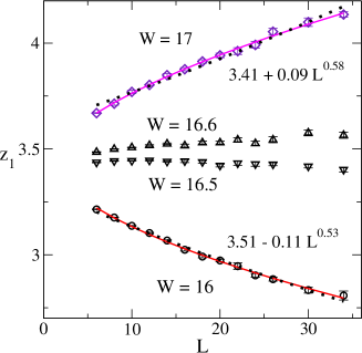
To support the result (3), Suslov used numerical data for parameter $z_{1}$ published in Ref. 2 and found that $L_{0}\approx 5$ (left Fig. 6 in 1 ). We show in Fig. 1 the same Figure with additional data for $24\leq L\leq 34$. Power fit $z_{1}(L)=a+bL^{\alpha}$ calculated for $W=16$ and $W=17$ supports the validity of the the relation (4).

Before testing the validity of Eq. (3) we have to notice the relation (2) between the localization length expressed in Eq. (3) and the parameter $z_{1}$ shown in Fig. 1. We fit our data for $z_{1}$ to the function

$$\zeta=\displaystyle{\frac{1}{a_{0}+a_{1}L}}$$ (5)

shown by dotted lines in Fig. 1. Comparing with Eq. (3) and using $y^{*}=z_{1c}^{-1}=3.48^{-1}$ (Fig. 2) we obtain $L_{0}\approx 8.6$ from $W=16$ data, but significantly different value $L_{0}\approx 17$ for $W=17$.

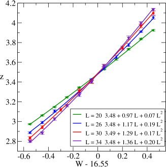
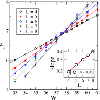
Although the power fit (4) is clearly better than the fit (5), Fig. 1 shows that the estimation of true scaling behavior might be difficult since various analytical functions seem to fit numerical data with sufficient accuracy. In the present case, the problem lies in the non-zero critical value $z_{1c}$. To avoid the ambiguity in the choice of the fitting function, we have to extract the critical value from numerical datajpa . When data for $z_{1}$ are plotted as a function of the disorder (Fig. 2), we can fit them by quadratic polynomial

$$z_{1}(W,L)=z_{1c}+\tau s(L)+\tau^{2}t(L)$$ (6)

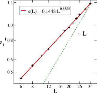
and calculate the $L$-dependence of the slope $s(L)$. From Eq. (3) we see that $s(L)$ should be a linear function of $L$, while Eq. (4) predicts power-law behavior $s(L)\sim L^{1/\nu}$. Figure 3 shows $s(L)$ as a function of $L$. The fit confirms the power-law dependence $s(L)\sim L^{1/\nu}$ with critical exponent $\nu\approx 1.56$, as obtained by other methods sc .

Figure 2: Quadratic fit (6) of $z_{1}(W-W_{c})$ for four values of the size $L$. The cross section determines $z_{1c}\approx 3.48$.

Figure 3: The $L$-dependence of the slope $s(L)\sim L^{1/\nu}$. The critical exponent $\nu=1.566$. Dashed line shows the linear $L$-dependence, predicted by Eq. (3).

III 5D model

For higher dimension, the following size dependence of the localization length at the critical point ($\tau=0$) was derived

$$\frac{\xi_{\rm 1D}}{L}=\left(\displaystyle{\frac{L}{a}}\right)^{(d-4)/3}.$$ (7)

In particular, for $d=5$ Eq. (7) gives

$$z_{1}(\tau=0)\sim L^{-1/3}$$ (8)

which means that the critical value of $z_{1}$ is not size independent but decreases to zero when $L\to\infty$.

Figure 4: The parameter $z_{1}(W)$ for various system size. For $W<57.5$, $z_{1}$ decreases when $L$ increases. There is no indication for the critical behavior described by Eq. (9)

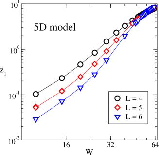
Since the localization length is finite in for $\tau>0$, the $\tau$-dependence of $z_{1}(L,\tau)$ for fixed $L$ must exhibit an infinite discontinuity at $\tau=0$:

$$z_{1}(\tau)\sim\left\{\begin{array}[]{ll}L^{-1/3}&\tau=0\\ L&\tau>0\end{array}\right.$$ (9)

We test numerically the size and disorder dependence of $z_{1}$. We show in Fig. 4 and 5 the disorder dependence of $z_{1}$ for fixed $L$. Our data in Fig. 4 do not indicate any discontinuity in the $L$ dependence. Contrary, $z_{1}$ is smooth analytical function of both parameters, $W$ and $L$.

For smaller disorder, $z_{1}$ is always decreasing function of $L$. This is typical for the metallic regime. However, $z_{1}$ does not depend on the size $L$ when $W=57.5$. This is consistent with the scaling equation (4). Insulating regime, where $z_{1}$ increases with the size $L$ is observed only when $W>57.5$ (Fig. 5).

Note that $z_{1}\approx 7$ for disorder $W\approx 57.5$. Therefore the localization length,

$$\xi_{\rm 1D}=\displaystyle{\frac{2}{z_{1}}L}$$ (10)

is much smaller than the size of the system and we do not expect that finite size effects play significant role although the size $L$ is much smaller than in 3D system.

Scaling analysis, similar to that for the 3D model enables us to find the critical exponent, $\nu_{\rm 5D}\approx 0.96$.

Figure 5: The 5D Anderson model: the parameter $z_{1}$ as a function of disorder $W$ for $L=4,5,6,7$ and $L=8$. Data indicate that $z_{1}$ does not depend on the size $L$ when $W\approx 57.5$. This value is considered as a critical disorder $W_{c}$ in the “standard” finite size scaling theory. Solid lines are fits $z_{1}(L)=z_{1}+s(L)(W-W_{c})$. Inset shows the $L$-dependence of the slope $s(L)\sim L^{1.0413}$. The original figure was published in 2 but new data for $L=8$ were added.

IV Conclusion

We showed that numerical data for the parameter $z_{1}$ do not agree with the predictions of the theory 1 . Both $z_{1}$ and the localization length are analytical continuous functions of the disorder $W$ and the size of the system $L$.

For the 3D system, we presented additional numerical data for larger system size $L\leq 24$ up to $L=34$. These new data confirm previous estimation of the critical exponent $\nu=1.56$.so ; jpa It is worth to mention that the same value of the critical exponent was obtained already 20 years ago with the use of numerical data for $L\leq 12$ only mac . We also note that the same value of the critical exponent was obtained from numerical analysis of other physical quantities: mean conductance, conductance distribution, inverse participation ratio 2 and also for critical points outside the band center 2 ; 4 . This value of critical exponent was recently verified experimentally 3 and calculated analytically gg .

References

- (1) I. M. Suslov, J. Exp. Theor. Phys. 114, 107 (2012).
- (2) A. MacKinnon and B. Kramer, Phys. Rev. Lett. 47, 1546 (1981).
- (3) K. Slevin and T. Ohtsuki, Phys. Rev. Lett. 78, 4083 (1997).
- (4) P. Markoš, acta physica slovaca 56, 561 (2006).
- (5) D. Vollhardt and P. Wölfle, in Electronic Phase Transitions ed. W. Hanke and Ya. V. Kopaev (Amsterdam, North-Holland) p. 1 (1992).
- (6) B. Kramer and A. MacKinnon, Rep. Prog. Phys. 56, 1469 (1993).
- (7) P. Markoš, J. Phys.: Condens. Matt. 7, 8361 (1995).
- (8) P. Markoš, J. Phys. A: Math. Gen. 33, L393 (2000).
- (9) A. MacKinnon, J. Phys. Condens. Matt. 6, 2511 (1994).
- (10) A. Croy et al.. Parallel Algorithms and Cluster Computing”, Lecture Notes in Computational Science and Engineerings (K. Hoffman, A. Meyer, eds.) Springer, Berlin, 203 (2006).
- (11) M. Lopez et al., Phys. Rev. Lett. 108, 095701 (2012); G. Lemairé et al., Phys. Rev. A 80, 043626 (2009).
- (12) A. M Garía-García and E. Cuevas. Phys. Rev. B 75, 174203 (2007).