GSI anomaly and spin-rotation coupling

Abstract

We propose a model in which a recently reported modulation in the decay of the hydrogenlike ions ¹⁴⁰Pr⁵⁸⁺, ¹⁴²Pm⁶⁰⁺ and ¹²²I⁵²⁺ arises from the coupling of rotation to the spin of electron and nucleus. The model shows that the spin-spin coupling of electron and nucleus does not contribute to the modulation and predicts that the anomaly cannot be observed if the motion of the ions is rectilinear, or if the ions are stopped in a target. It also supports the notion that the modulation frequency is proportional to the inverse of the atomic mass and that no modulation is expected for the $\beta^{+}$-decay.

I Introduction

Experiments carried out at the storage ring ESR of GSI in Darmstadt GSI ; GSIb ; geissel reveal an oscillation in the orbital electron capture and subsequent decay of hydrogenlike ¹⁴⁰Pr⁵⁸⁺, ¹⁴²Pm⁶⁰⁺ and ¹²²I⁵²⁺. The modulation has a period of $7.069(8)\,$s, $7.10(22)\,$s and $6.1\,$s respectively in the laboratory frame and is superimposed on the expected exponential decay. The ”zero hypothesis” of a pure experimental decay has been excluded at the $99\%$ C.L. and periodic instabilities in the storage ring and detection apparatus also seem improbable causes of the modulation. The effect has been extensively studied in literature mixing ; giuntiPLB ; merleIOP ; merlePRC .

We show, in the model proposed below, that a modulation arises in the probability that the system, initially in a superposition of hyperfine states ($F=3/2$ and $F=1/2$), finds itself again in such a superposition of hyperfine states after injection into the storage ring. The modulation has its origin in the spin-dependent part of the Thomas precession, and is compatible with the observed ESR modulation. The EC decay occurs for states with spin $F=1/2$ because decay from the spin $3/2$ state is forbidden by the conservation of the $F$ quantum number GSIb . We stress that the present paper differs in essential ways from lambiase08 because it takes into account all the relevant features of the GSI experiment, such as bound states kinematics, dragging effects, Thomas precessions of nucleus and electron and QED and derives the probability of the observed modulation from the time evolution of nucleus plus electron once this system is injected in the storage ring.

The full Hamiltonian that describes the behavior of nucleus and bound electron in the external field ${\bf B}$ of the ring is $H=H_{0}+H_{1}$, where $H_{0}$ contains all the usual standard terms (Coulomb potential, spin-orbit coupling, etc.), and $H_{1}$ is (in units $\hbar=c=1$)

$$H_{1}=-{\cal A}\,{\bf s}\cdot{\bf I}-{\bf s}\cdot{\bm{\Omega}}_{e}-{\bf I}\cdot{\bm{\Omega}}_{n}\,,$$ (1)

where ${\cal A}\simeq Z^{3}\displaystyle{\frac{4\alpha^{4}g_{n}}{3}}\sim N\times 10^{14}\mbox{Hz}\,,N\sim{\cal O}(1)$ is the strength of spin-spin coupling, while

$${\bm{\Omega}}_{e}\equiv{\bm{\omega}}_{g_{e}}+{\bm{\omega}}_{Th}^{(e)}-{\bm{\omega}}_{c}^{(e)}\,,$$ (2)

$${\bm{\Omega}}_{n}\equiv{\bm{\omega}}_{g_{n}}+{\bm{\omega}}_{Th}^{(n)}-{\bm{\omega}}_{c}^{(n)}\,,$$ (3)

represent the precession of the electron spin and the usual spin precession of the nucleus in its motion in a storage ring that is assumed circular for simplicity. In (2) and (3), ${\bm{\omega}}_{g_{e,n}}$ are the electron and nucleus spin precession frequencies due to the respective magnetic moments $g_{e,n}$ and ${\bm{\omega}}_{c}^{(e,n)}$ are the angular cyclotron frequencies. The explicit expressions of all these quantities are given below. We refer (1) to a frame rotating about the $x_{3}$-axis in the clockwise direction of the ions, with the $x_{2}$-axis tangent to the ion orbit in the direction of its momentum and write ${\bf B}=B{\bf\hat{u}}_{3}$, where $B=1.197$T is the GSI value (we are assuming that this is the average value over the circumference).

The Thomas precession ${\bm{\omega}}_{Th}^{(e,n)}$ is related to the standard spin-rotation coupling that can be derived, for the electron, from the spin connection coefficients of the Dirac equation in a rotating frame jackson ; pap . In our derivation, we neglect any stray electric fields and electric fields needed to stabilize the nucleus orbits, as well as all other effects which could affect the Thomas precession silenko .

We indicate by ${\bm{\beta}}$ and ${\bm{\beta}}_{n}$ the velocities of electron and nucleus relative to the lab frame. Using the composition of velocities, the Lorentz factor $\gamma=1/\sqrt{1-{\bm{\beta}}^{2}}$ of the electron can be written in the form $\gamma=\gamma_{n}\gamma_{e|n}(1+\Pi)$, where $\Pi={\bm{\beta}_{n}}\cdot{\bm{\beta}_{e|n}}=\beta_{n}\beta_{e|n}\cos\theta$, ${\bm{\beta}}_{e|n}$ is the velocity of the electron relative to the nucleus, $\gamma_{n}=1/\sqrt{1-{\bm{\beta}}_{n}^{2}}$, and $\gamma_{e|n}=1/\sqrt{1-{\bm{\beta}}_{e|n}^{2}}$. The explicit expression of ${\bm{\beta}}$ is also useful

$${\bm{\beta}}=\frac{1}{\gamma_{n}(1+\Pi)}\left[{\bm{\beta}}_{e|n}+\frac{\gamma_{n}^{2}\Pi}{\gamma_{n}+1}\,{\bm{\beta}}_{n}+\gamma_{n}{\bm{\beta}}_{n}\right]\,.$$ (4)

The Thomas precession of the electron in the lab frame is given by ${\bm{\omega}}_{Th}=-\displaystyle{\frac{\gamma^{2}}{\gamma+1}\frac{d{\bm{\beta}}}{dt}\wedge{\bm{\beta}}}$. The field $\bf B$ in the lab frame (where $\bf E=0$) is transformed to the nucleus rest frame and gives ${\bf E}^{\prime}=\gamma_{n}{\bm{\beta}}_{n}\wedge{\bf B}$ and ${\bf B}^{\prime}=\gamma_{n}{\bf B}$ on account of ${\bm{\beta}}_{n}\cdot{\bf B}=0$. The equations of motion are $\displaystyle{\frac{d{\bm{\beta}}_{e|n}}{dt_{n}}}=\displaystyle{\frac{{\bf f}_{e|n}}{\gamma_{e|n}m}}-\displaystyle{\frac{{\bm{\beta}}_{e|n}}{\gamma_{e|n}}\frac{{\bm{\beta}}_{e|n}\cdot{\bf f}_{e|n}}{m}}$ for the electron with respect to the nucleus and $\displaystyle{\frac{d{\bm{\beta}}_{n}}{dt}}=\displaystyle{\frac{Q}{M\gamma_{n}}}\,{\bm{\beta}}_{n}\wedge{\bf B}$ for the nucleus with respect to the lab frame. Here ${\bf f}_{e|n}=-e({\bf E}^{\prime}+{\bm{\beta}}_{e|n}\wedge{\bf B}^{\prime})=-e\gamma_{n}({\bm{\beta}}_{e|n}+{\bm{\beta}}_{n})\wedge{\bf B}$. Using $dt=\gamma_{n}(1+\Pi)dt_{n}$, taking ${\bm{\beta}}_{e|n}\cdot{\bf B}=0$, ${\bf E}_{e|n}\wedge{\bf\beta}_{e|n}=0$ and ${\bf E}_{e|n}\wedge{\bf\beta}_{n}=0$ (averaged over the decay time of the ion in the storage ring), we find $\displaystyle{\frac{d{\bm{\beta}}_{e|n}}{dt}}=-\displaystyle{\frac{e}{m}\frac{1}{\gamma_{e|n}(1+\Pi)}[{\bm{\beta}}_{e|n}+{\bm{\beta}}_{n}]\wedge{\bf B}}$. Neglecting spin-orbit coupling, ${\bm{\omega}}_{Th}$ can be written as

$${\bm{\omega}}_{Th}=\frac{e{\bf B}}{m}\frac{1}{\gamma_{e|n}\gamma_{n}}I_{e}-\frac{Q{\bf B}}{M}\frac{1}{\gamma_{n}}I_{Q}\,,$$ (5)

where

$$I_{e}\equiv\frac{\displaystyle{(\gamma_{e|n}\gamma_{n})^{2}\left({\bm{\beta}}_{n}^{2}+\frac{{\bm{\beta}}_{e|n}^{2}}{\gamma_{n}}+2\Pi+\frac{\gamma_{n}\Pi^{2}}{\gamma_{n}+1}-Y\right)}}{(1+\Pi)[\gamma_{e|n}\gamma_{n}(1+\Pi)+1]}\,,$$

$$I_{Q}\equiv\frac{(\gamma_{e|n}\gamma_{n})^{2}\displaystyle{\left[{\bm{\beta}}_{n}^{2}\left(1+\frac{\gamma_{n}\Pi}{\gamma_{n}+1}\right)^{2}-X\right]}}{\gamma_{e|n}\gamma_{n}(1+\Pi)+1}\,,$$

$$Y\equiv\frac{{\bm{\beta}}_{e|n}^{2}[\gamma_{n}(2-\cos^{2}\theta)-\sin^{2}\theta]}{3\gamma_{n}^{2}},X\equiv\frac{{\bm{\beta}}_{e|n}^{2}{\bm{\beta}}_{n}^{2}\sin^{2}\theta}{3(\gamma_{n}+1)}\,.$$

The coupling of the electron magnetic moment ${\bm{\mu}}_{e}=-\displaystyle{\frac{g_{e}}{2}\frac{e}{m_{e}}}{\bf s}$ with the magnetic field is described by

$$H_{g_{e}}=\frac{1}{\gamma}{\bm{\mu}}_{e}\cdot{\bf B}^{\prime\prime}={\bm{\mu}}_{e}\cdot\left[{\bf B}-\frac{\gamma}{\gamma+1}{\bm{\beta}}({\bm{\beta}}\cdot{\bf B})\right]\,.$$

Keeping only the quadratic term in ${\bm{\beta}}_{e|n}$ and using ${\bm{\beta}}({\bm{\beta}}\cdot{\bf B})=\displaystyle{\frac{({\bm{\beta}}_{e|n}\cdot{\hat{\bf u}_{3}})^{2}}{\gamma_{n}^{2}(1+\Pi)^{2}}\,{\bf B}}$, we obtain

$$H_{g_{e}}=\Upsilon\,{\bm{\mu}}_{e}\cdot{\bf B}\,,\quad\Upsilon\equiv 1-\frac{\gamma_{e|n}^{2}({\bm{\beta}}_{e|n}\cdot{\hat{\bf u}_{3}})^{2}}{\gamma(\gamma+1)}\,,$$ (6)

and from it $d{\bf s}/dt=i[H_{g_{e}},{\bf s}]={\bm{\omega}}_{g_{e}}\wedge{\bf s}={\Upsilon}{\bm{\mu}}_{e}\wedge{\bf B}$ which yields

$${\bm{\omega}}_{g_{e}}=-\displaystyle{\frac{g_{e}e}{2m_{e}}\,{\Upsilon}\,{\bf B}}\,.$$ (7)

In order to refer the spin precession to the particle orbit, the effective cyclotron frequency ${\bm{\omega}}_{c}^{(e)}$ must now be subtracted. Its value is obtained by computing the instantaneous acceleration $d{\bm{\beta}}/dt=\omega_{e}^{(c)}\beta{\hat{\bf u}}_{1}$. Omitting terms like ${\bf a}_{e|n}=\frac{q}{m_{e}}{\bf E}_{e|n}$, ${\bm{\beta}}_{e|n}\wedge{\bf B}$ and $[{\bf B}\cdot({\bm{\beta}}_{e|n}\wedge{\bm{\beta}}_{n})]{\bm{\beta}}_{n}$ that vanish when averaged, as already pointed out, we find

$${\bm{\omega}}_{c}^{(e)}=\left[-\frac{eB}{m_{e}}\frac{\beta_{n}}{\beta}\frac{1-({\bm{\beta}}_{e|n}\cdot{\hat{\bf u}}_{1})^{2}}{\gamma_{e|n}\gamma_{n}(1+\Pi)^{2}}+\frac{QB}{M}\frac{\beta_{n}}{\gamma_{n}\beta}\Xi_{n}\right]{\bf u}_{3}\,,$$ (8)

where $\Xi_{n}\equiv\displaystyle{\frac{1}{\gamma_{n}+1}\left(1+\frac{\gamma_{n}\Pi}{\gamma_{n}+1}\right)}$ and

$$\beta=\sqrt{\frac{{\bm{\beta}}_{n}^{2}+\frac{{\bm{\beta}}_{e|n}^{2}}{\gamma_{n}^{2}}+2\Pi+\Pi^{2}}{(1+\Pi)^{2}}}\,.$$

From (2),(5) and (8) we obtain

$${\bm{\Omega}}_{e}=-\frac{e{\bf B}}{m_{e}}\left(\frac{g_{e}}{2}{\Upsilon}-\frac{I_{e}}{\gamma_{e|n}\gamma_{n}}-U\right)-\frac{Q{\bf B}}{M}\frac{I_{Q}+V}{\gamma_{n}}\,,$$ (9)

where $\Upsilon$ is defined in (6) and

$$U\equiv\frac{1-({\bm{\beta}}_{e|n}\cdot{\hat{\bf u}_{1}})^{2}}{\gamma_{e|n}\gamma_{n}(1+\Pi)^{2}}\frac{\beta_{n}}{\beta}\,,V\equiv\frac{\beta_{n}}{\beta(1+\Pi)}\left(1+\frac{\gamma_{n}\Pi}{\gamma_{n}+1}\right)\,.$$ (10)

Notice that the standard result $\Omega_{e}=-e{\bf B}a_{e}/m_{e}$, where $a_{e}=(|g_{e}|-2)/2$ is the electron magnetic moment anomaly, is recovered in the limit $Q=0$.

The calculation of $g_{e}$-factors, based on bound state (BS) QED, can be carried out with accuracy even though, in our case, the expansion parameter is $Z\alpha\simeq 0.4$. The BS-QED calculation gives vogel ; blundell

$$g_{e}^{b}=2\left[\frac{1+2\sqrt{1-(\alpha Z)^{2}}}{3}+\frac{\alpha}{\pi}C^{(2)}(\alpha Z)\right]\,,$$ (11)

where $C^{(2)}(\alpha Z)\simeq\frac{1}{2}+\frac{1}{12}(\alpha Z)^{2}+\frac{7}{2}(\alpha Z)^{4}$. From (11) we obtain the values $a_{e}\simeq-0.065122$, $a_{e}\simeq-0.0682112$ and $a_{e}=0.0505352$ for ¹⁴⁰Pr⁵⁸⁺, ¹⁴²Pm⁶⁰⁺ and ¹²²I⁵²⁺ respectively. The addition of more expansion terms CODATA does not change these results appreciably.

Consider now the nucleus with spin ${\bf I}$. The terms of (3) are ${\bm{\omega}}_{g_{n}}=\displaystyle{g_{n}\mu_{N}}{\bf B}$, where $\mu_{N}=\displaystyle{\frac{|e|}{2m_{p}}}$, ${\bm{\omega}}_{Th}^{(n)}=-\displaystyle{\frac{\gamma_{n}-1}{\gamma_{n}}\frac{Q{\bf B}}{M}}$, ${\bm{\omega}}_{c}^{(n)}=\displaystyle{\frac{Q{\bf B}}{M\gamma_{n}}}$ and give

$${\bm{\Omega}}_{n}=\frac{Q{\bf B}}{M}\left(\frac{g_{n}}{2}\frac{A}{Z}-1\right)\,.$$ (12)

II Probability and modulation

Let $|I,m_{I}\rangle_{I}$ and $|s,m_{s}\rangle_{s}$ be the eigenstates of the operators ${\bf\hat{I}}$ and ${\bf\hat{s}}$. The total angular momentum operator is ${\bf\hat{F}}={\bf\hat{s}}+{\bf\hat{I}}$. The angular momentum $F$ assumes the values $F=3/2,1/2$, $m_{F=3/2}=\pm 3/2,\pm 1/2$, and $m_{F=1/2}=\pm 1/2$ because $I=1$, $m_{I}=\pm 1,0$ and $s=1/2$, $m_{s}=\pm 1/2$. By making use of the raising and lowering operators ${\bf\hat{F}}_{\pm}={\bf\hat{I}}_{\pm}+{\bf\hat{s}}_{\pm}$, we construct the normalized and orthogonal states

$$\phi_{1} \equiv \Big{|}\frac{3}{2},\frac{3}{2}\rangle_{F}=|1,1\rangle_{I}\Big{|}\frac{1}{2},\frac{1}{2}\rangle_{s}$$

$$\phi_{2} \equiv \Big{|}\frac{3}{2},\frac{1}{2}\rangle_{F}=\sqrt{\frac{2}{3}}|1,0\rangle_{I}\Big{|}\frac{1}{2},\frac{1}{2}\rangle_{s}+\sqrt{\frac{1}{3}}|1,1\rangle_{I}\Big{|}\frac{1}{2},-\frac{1}{2}\rangle_{s}$$

$$\phi_{3} \equiv \Big{|}\frac{3}{2},-\frac{1}{2}\rangle_{F}=$$

$$= \sqrt{\frac{2}{3}}|1,0\rangle_{I}\Big{|}\frac{1}{2},-\frac{1}{2}\rangle_{s}+\sqrt{\frac{1}{3}}|1,-1\rangle_{I}\Big{|}\frac{1}{2},\frac{1}{2}\rangle_{s}$$

$$\phi_{4} \equiv \Big{|}\frac{3}{2},-\frac{3}{2}\rangle_{F}=|1,-1\rangle_{I}\Big{|}\frac{1}{2},-\frac{1}{2}\rangle_{s}$$

$$\phi_{5} \equiv \Big{|}\frac{1}{2},\frac{1}{2}\rangle_{F}=\sqrt{\frac{1}{3}}|1,0\rangle_{I}\Big{|}\frac{1}{2},\frac{1}{2}\rangle_{s}-\sqrt{\frac{2}{3}}|1,1\rangle_{I}\Big{|}\frac{1}{2},-\frac{1}{2}\rangle_{s}$$

$$\phi_{6} \equiv \Big{|}\frac{1}{2},-\frac{1}{2}\rangle_{F}=$$

$$= -\sqrt{\frac{2}{3}}|1,-1\rangle_{I}\Big{|}\frac{1}{2},\frac{1}{2}\rangle_{s}+\sqrt{\frac{1}{3}}|1,0\rangle_{I}\Big{|}\frac{1}{2},-\frac{1}{2}\rangle_{s}\,.$$

The ($6\times 6$) matrix with elements $\langle\phi_{i}|{\hat{H}}_{1}|\phi_{j}\rangle$ has the eigenvalues

$$\lambda_{1,4} = -\frac{\cal A}{2}\pm\left(\frac{\Omega_{e}}{2}+\Omega_{n}\right)\,,$$

$$\lambda_{2,3} = \frac{\cal A}{4}\mp\frac{\Omega_{n}}{2}-\frac{\sqrt{\Delta_{\pm}}}{4}\,,\,\,\lambda_{5,6}=\frac{\cal A}{4}\mp\frac{\Omega_{n}}{2}+\frac{\sqrt{\Delta_{\pm}}}{4}\,,$$

where

$$\Delta_{\pm}=9{\cal A}^{2}\pm 4{\cal A}\Omega_{e}\mp 4{\cal A}\Omega_{n}+4(\Omega_{e}-\Omega_{n})^{2}\,,$$

and the corresponding eigenstates $|i\rangle$ ($i=1,\ldots,6$)

$$|1,4\rangle = \phi_{1,4}\,,\quad|2,5\rangle=\frac{B_{\pm}}{\sqrt{1+B_{\pm}^{2}}}\phi_{2}+\frac{1}{\sqrt{1+B_{\pm}^{2}}}\phi_{5}\,,$$

$$|3,6\rangle = -\frac{A_{\pm}}{\sqrt{1+A_{\pm}^{2}}}\phi_{3}+\frac{1}{\sqrt{1+A_{\pm}^{2}}}\phi_{6}\,,$$

where

$$A_{\pm}=\displaystyle{\frac{9{\cal A}-2\Omega_{e}+2\Omega_{n}\pm 3\sqrt{\Delta_{-}}}{4\sqrt{2}\,(\Omega_{e}-\Omega_{n})}}\,,$$

and

$$B_{\pm}=\displaystyle{\frac{9{\cal A}+2\Omega_{e}-2\Omega_{n}\pm 3\sqrt{\Delta_{+}}}{4\sqrt{2}\,(\Omega_{e}-\Omega_{n})}}\,.$$

In the limit ${\cal A}\gg\Omega_{e,n}$ we obtain

$$|i\rangle\simeq|\phi_{i}\rangle\,,$$ (13)

and

$$\lambda_{1}-\lambda_{2}=\lambda_{2}-\lambda_{3}=\frac{\lambda_{1}-\lambda_{3}}{2}=-\frac{\Omega_{e}+2\Omega_{n}}{3}\,,\quad\lambda_{1}-\lambda_{4}=-\Omega_{e}+2\Omega_{n}\,,$$ (14)

$$\lambda_{5}-\lambda_{6}=\frac{\Omega_{e}-4\Omega_{n}}{3}\,.$$ (15)

Notice that in these expressions the ${\cal A}$-terms coming from the spin-spin coupling cancel out.

II.1 Modulation induced by quantum beats

These results must be now applied to the GSI experiment. Since the heavy nucleus decays via EC, only the states with $F=1/2$ are relevant. For simplicity we confine ourselves to the Hilbert subspace spanned by the states $\{|5\rangle,|6\rangle\}$. Here we follow giuntiPLB (see also merleIOP ; merlePRC ). The decay processes involved in the GSI experiment ${}^{140}\text{Pr}^{\,58+}\to{}^{140}\text{Ce}^{\,58+}+\nu_{e}$, ${}^{142}\text{Pm}^{\,60+}\to{}^{140}\text{Nd}^{\,58+}+\nu_{e}$, and ${}^{122}\text{I}^{\,52+}\to{}^{122}\text{Te}^{\,52+}+\nu_{e}$, can be schematically represented as

$${\mathbb{I}}\quad\to\quad{\mathbb{F}}+\nu_{e}\,,$$ (16)

with obvious meaning of the symbols. At the initial instant $t=0$ (before injection into the ESR) the system nucleus-electron is produced in a superposition of the states $\{|5\rangle,|6\rangle\}$,

$$|{\mathbb{I}}(0)\rangle=\sum_{a=5}^{6}c_{a}|a\rangle=c_{5}|5\rangle+c_{6}|6\rangle\,.$$

with $|c_{5}|^{2}+|c_{6}|^{2}=1$. If one assumes, for simplicity, that the two states with energies $\lambda_{5}$ and $\lambda_{6}$ decay with the same rate $\Gamma$, at the time $t$ the system evolves to the state

$$|{\mathbb{I}}(t)\rangle=e^{-\Gamma t/2}\left(c_{5}e^{-i\lambda_{5}t}|5\rangle+c_{6}e^{-i\lambda_{6}t}|6\rangle\right)\,.$$

The probability of EC at time $t$ reads

$$P_{EC}(t)=e^{-\Gamma t}|\langle\nu_{e},{\mathbb{F}}|S|{\mathbb{I}}(t)\rangle|^{2}=e^{-\Gamma t}{\bar{P}}_{EC}\left[1+a_{56}\cos\left(\omega_{56}t+\varsigma\right)\right]\,,$$ (17)

where (see Eq. (15))

$$\omega_{56}=|\lambda_{5}-\lambda_{6}|=\frac{\Omega_{e}-4\Omega_{n}}{3}\,,$$ (18)

${\bar{P}}_{EC}=|\langle\nu_{e},{\mathbb{F}}|S|5\rangle|^{2}=|\langle\nu_{e},{\mathbb{F}}|S|6\rangle|^{2}$, $a_{56}=2|c_{5}||c_{6}|$, and finally $S$ is the interaction operator. The phase $\varsigma$ comes form possible phase differences of the amplitude $c_{1}$ and $c_{2}$ and of $|\langle\nu_{e},{\mathbb{F}}|S|5\rangle|$ and $|\langle\nu_{e},{\mathbb{F}}|S|6\rangle|$. As (17) and (18) show, the modulation of the decay probability does not depend on ${\cal A}$.

II.2 Estimate of $\gamma_{e|n}$

We now compare the frequencies $\omega_{56}/2\pi$, given by (18), with the experimental values $\sim 0.14\,$ Hz found for ¹⁴⁰Pr⁵⁸⁺ and ¹⁴²Pm⁶⁰⁺ and $\sim 0.16\,$Hz for ¹²²I⁵²⁺ and consider first the case $\omega_{56}=\lambda_{5}-\lambda_{6}$. We find

$$\frac{|e|B}{3m_{p}}\left[\frac{m_{p}}{m_{e}}\left({\bar{\Upsilon}}(a_{e}+1)-\frac{{\bar{I}}_{e}}{\gamma_{e|n}\gamma_{n}}-{\bar{U}}\right)+\frac{I_{Q}+{\bar{V}}}{\gamma_{n}}\frac{Z}{A}+4\frac{Z}{A}\left(\frac{g_{n}}{2}\frac{A}{Z}-1\right)\right]=2\pi\,0.14\,\mbox{Hz}\,,$$ (19)

where a bar on top means average values. These are computed by first expanding the quantities $I_{e,Q}$, $\Upsilon$, $U$ and $V$ in terms of $\Pi<1$ and then averaging over the angle by means of $\langle\cos^{n}\theta\rangle=\frac{1+(-1)^{n}}{2(n+1)}$. Using $({\bm{\beta}}_{e|n}\cdot{\hat{\bf u}}_{i})^{2}=\frac{1}{3}{\bm{\beta}}_{e|n}^{2}$, $i=1,2,3$, $\gamma_{n}^{\text{(Pr, Pm, I)}}=1.43$, $g_{n}^{\text{(Pr,Pm)}}=2.5$, $g_{n}^{\text{(I)}}=0.94$, up to ${\cal O}(\Pi^{6})$ we obtain from (19) the numerical solutions (see Fig. 1)

$$\gamma^{(\text{Pr})}_{e|n}\sim 1.07904\,,\quad\gamma^{(\text{Pm})}_{e|n}\sim 1.08435\,,\quad\gamma^{(\text{I})}_{e|n}\sim 1.05902\,,$$ (20)

which must be compared with the Lorentz factors of the bound electron in the Bohr model $\gamma^{(\text{Pr})}_{e|n}\sim 1.0970$, $\gamma^{(\text{Pm})}_{e|n}\sim 1.1040$, and $\gamma^{(\text{I})}_{e|n}\sim 1.0776$. The values (20) imply that the binding energies $E=T+E_{p}=-m[1-\gamma_{e|n}+(\alpha Z)^{2}]$, where $T$ ad $E_{p}$ are kinetic and potential energies of the bound electron, are given by

$$E^{(\text{Pr})}\sim-54.4\text{keV},\quad E^{(\text{Pm})}\sim-58.2\text{keV},\quad E^{(\text{I})}\sim-46.3\text{keV},$$

in agreement with the values

$$E^{(\text{Pr})}_{R}=-49.5\text{keV},\quad E^{(\text{Pm})}_{R}=-53.1\text{keV},\quad E^{(\text{I})}_{R}=-39.6\text{keV},$$ (21)

derived from the relativistic equation zuber

$$E_{R}=-\displaystyle{\frac{RZ^{2}}{n^{2}}\left[1+\frac{(\alpha Z)^{2}}{n}\left(1-\frac{3}{4n}\right)\right]}\,,$$ (22)

where $R=13.6057$eV and $n=1$.

III Conclusions

In this paper we explain the GSI anomaly by means of a semiclassical model based on the Thomas precession of spins. The model has the following consequences: 1) It avoids all criticisms raised in faber and in fastermann because the Hamiltonians are essentially different. 2) There is no modulation in the $\beta^{+}$-decay branch kienle . This because the Thomas precession, when computed only for a decaying charged nucleus gives rise to a frequency $\Omega_{n}\sim eB/m_{p}\sim 10^{7}$ Hz and the probability $\sim e^{-\Gamma t}[1+a\cos(\Omega_{n}t)]$. The high frequency modulation term averages out to zero, and the probability obeys the standard exponential decay. 3) The GSI oscillations disappear when $B=0$. 4) The model is consistent with experiments on EC decays of neutral atoms in solid environments that have shown no oscillations/modulations vetter . 5) The model predicts that $\omega_{56}\sim A^{-1}$ if the three terms on the l.h.s. of (19) are of the same order of magnitude (notice however that the $A$-terms only affect the third digit of $\gamma_{e|n}$ and are not, therefore, a real discriminating feature of our model). 6) The model is consistent with the absence of a periodic transfer from active $(F=1/2)$ to sterile $(F=3/2)$ states.

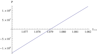
Figure 1: P is defined by P $\equiv\frac{|e|{\bf B}}{3m_{p}}\Big{[}\frac{m_{p}}{m_{e}}\Big{(}{\tilde{\Upsilon}}(a_{e}+1)-\frac{I_{e}}{\gamma_{e|n}\gamma_{n}}-{\tilde{U}}\Big{)}+$ $\frac{I_{Q}+{\tilde{V}}}{\gamma_{n}}\frac{Z}{A}+4\frac{Z}{A}\Big{(}\frac{g_{n}}{2}\frac{A}{Z}-1\Big{)}\Big{]}-2\pi\,0.14$ Hz (19), with ${\tilde{\Upsilon}}$, ${\tilde{U}}$ and ${\tilde{V}}$ given by (10). The value of the unknown $\gamma_{e|n}$ is obtained from $P=0$ by using the experimental data and corresponds to the central value of the range $6.98s\lesssim T\lesssim 7.06s$ The plot refers to Pr. Similar plots can be obtained for Pm and I.