Ground-state phase diagram of the spin-1/2 square-lattice J1-J2 model with plaquette structure

Abstract

Using the coupled cluster method for high orders of approximation and Lanczos exact diagonalization we study the ground-state phase diagram of a quantum spin-1/2 $J_{1}$-$J_{2}$ model on the square lattice with plaquette structure. We consider antiferromagnetic ($J_{1}>0$) as well as ferromagnetic ($J_{1}<0$) nearest-neighbor interactions together with frustrating antiferromagnetic next-nearest-neighbor interaction $J_{2}>0$. The strength of inter-plaquette interaction $\lambda$ varies between $\lambda=1$ (that corresponds to the uniform $J_{1}$-$J_{2}$ model) and $\lambda=0$ (that corresponds to isolated frustrated 4-spin plaquettes). While on the classical level ($s\to\infty$) both versions of models (i.e., with ferro- and antiferromagnetic $J_{1}$) exhibit the same ground-state behavior, the ground-state phase diagram differs basically for the quantum case $s=1/2$. For the antiferromagnetic case ($J_{1}>0$) Néel antiferromagnetic long-range order at small $J_{2}/J_{1}$ and $\lambda\gtrsim 0.47$ as well as collinear striped antiferromagnetic long-range order at large $J_{2}/J_{1}$ and $\lambda\gtrsim 0.30$ appear which correspond to their classical counterparts. Both semi-classical magnetic phases are separated by a nonmagnetic quantum paramagnetic phase. The parameter region, where this nonmagnetic phase exists, increases with decreasing of $\lambda$. For the ferromagnetic case ($J_{1}<0$) we have the trivial ferromagnetic ground state at small $J_{2}/|J_{1}|$. By increasing of $J_{2}$ this classical phase gives way for a semi-classical plaquette phase, where the plaquette block spins of length $s=2$ are antiferromagnetically long-range ordered. Further increasing of $J_{2}$ then yields collinear striped antiferromagnetic long-range order for $\lambda\gtrsim 0.38$, but a nonmagnetic quantum paramagnetic phase $\lambda\lesssim 0.38$.

I Introduction

The spin-1/2 quantum Heisenberg antiferromagnet with nearest-neighbor (NN), $J_{1}>0$, and next-nearest-neighbor (NNN) bonds, $J_{2}\geq 0$, on the square lattice has attracted much interest (see, e.g., Refs. chandra88, ; dagotto89, ; schulz, ; richter93, ; richter94, ; zhito96, ; Trumper97, ; bishop98, ; singh99, ; sushkov01, ; capriotti01, ; Sir:2006, ; Schm:2006, ; darradi08, ; sousa, ; bishop08, ; xxz, ; ortiz, ; singh2009, ; cirac2009, ; ED40, ; fprg, ; cirac2010, ; balents2011, ; verstrate2011, ) as a canonical model to study the interplay between frustration and quantum fluctuations. In particular, the quantum phase transitions inherent in this model as well as the nature of its quantum paramagnetic phase in the region $0.4\lesssim J_{2}/J_{1}\lesssim 0.6$ is a matter of intensive debate. The Néel antiferromagnetic (NAF) long-range order (LRO) at small $J_{2}/J_{1}$ and the collinear striped antiferromagnetic (CAF) LRO at large $J_{2}/J_{1}$ correspond to their classical counterparts, however, the sublattice magnetization is reduced by quantum fluctuations.

Motivated by recent investigations on quasi-two-dimensional frustrated magnetic materials with ferromagnetic (FM) NN bonds e.g., Pb₂VO(PO₄)₂,kaul04 ; jmmm07 ; carretta2009 ; enderle ; nath SrZnVO(PO₄)₂,rosner09 ; rosner09a ; enderle ; carretta2011 BaCdVO(PO₄)₂,nath2008 ; carretta2009 ; rosner09 the FM $J_{1}$-$J_{2}$ model ($J_{1}<0,J_{2}\geq 0$) has recently been studied.shannon04 ; shannon06 ; sindz07 ; schmidt07 ; schmidt07_2 ; sousa ; shannon09 ; sindz09 ; haertel10 ; richter10 ; momoi2011 ; cabra2011 Although on the classical level the ground state (GS) phase diagrams of both variants of the $J_{1}$-$J_{2}$ model are quite similar, the GS properties of the quantum model with $J_{1}<0$ are basically different from those for $J_{1}>0$. Currently, the GS properties of the FM model around $J_{2}/|J_{1}|=0.5$ are under controversial debate. On the one hand in Refs. shannon06, and momoi2011, arguments for a nematic phase separating the classical FM and the semi-classical CAF phases are given, on the other hand in Refs. richter10, and cabra2011, an intermediate quantum paramagnetic GS phase is not found (or it exists in a very small parameter region around $J_{2}\sim 0.4|J_{1}|$, only). Hence, a direct first-order transition between the FM GS and the GS with CAF LRO at $J_{2}\sim 0.4|J_{1}|$ could take place.richter10 ; cabra2011

Quantum phase transitions can also occur by competition between antiferromagnetic (AFM) NN bonds of different strength, i.e., without frustration. One example is the local singlet formation in dimerized Heisenberg models, see e.g. Ref. hjs, and references therein. As a certain extension to dimerized models the square-lattice Heisenberg model with a plaquette structure has been considered,singh99 ; voigt02 ; ueda07 ; fabricio08 ; wenzel08 ; wenzel09 ; fledderjohann09 where local quadrumer singlet formation can destroy NAF LRO.

However, for the description of real materials a modification of the $J_{1}$-$J_{2}$ model might be necessary. For example, for PbZnVO(PO₄)₂ a spatially anisotropy model has been derived,rosner2010 whereas for (CuCl)LaNb₂O₇kageyama05 a $J_{1}$-$J_{2}$ model with additional plaquette structure was proposed in Ref. ueda07, . This plaquette model, however, has been questioned recently by Rosner and coworkers.rosner_co

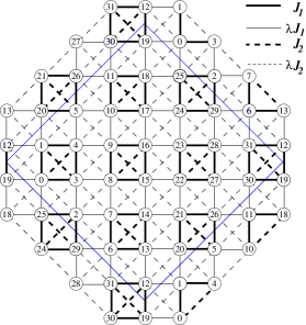
In this paper we consider the $J_{1}$-$J_{2}$ model on the square lattice with plaquette structure (see Fig. 1) merging this way the two mechanisms to destroy magnetic LRO, namely frustration and local singlet formation. Moreover, the model we will consider corresponds to that proposed in Ref. ueda07, for (CuCl)LaNb₂O₇. The Hamiltonian of our model is given by

$$H=\sum_{a=0}^{1}(\delta_{0a}+\delta_{1a}\lambda)\left(J_{1}\sum_{\langle ij\rangle_{a}}{\bf s}_{i}{\bf s}_{j}+J_{2}\sum_{\langle\langle ij\rangle\rangle_{a}}{\bf s}_{i}{\bf s}_{j}\right),$$ (1)

where the sum is taken over the nearest ($\langle\cdots\rangle$) and next-nearest ($\langle\langle\cdots\rangle\rangle$) neighbors, and $\delta_{ab}$ is the Kronecker symbol. We consider FM and AFM NN bonds $J_{1}=\pm 1$ and AFM (i.e. frustrating) NNN bonds $J_{2}\geq 0$. The intra- ($a=0$) and inter-plaquette interaction ($a=1$) differ by the factor $\lambda$. The case $\lambda=1$ corresponds to the standard uniform $J_{1}$-$J_{2}$ model on the square lattice, whereas the limit $\lambda=0$ describes unconnected 4-spin $J_{1}$-$J_{2}$ plaquettes. For the parameter $\lambda$ we consider the interval $\lambda\in[0,1]$ this way interpolating between a system of isolated plaquettes and the uniform $J_{1}$-$J_{2}$ model.

Figure 1: The two-dimensional spin $1/2$ $J_{1}$-$J_{2}$ finite square lattice of $N=32$ sites (periodic boundary conditions) with plaquette structure (see Eq. (1)); solid lines - NN bonds $J_{1}$ (thick) and $\lambda J_{1}$ (thin), dashed lines NNN bonds $J_{2}$ (thick) and $\lambda J_{2}$ (thin).

The model (1) has been studied previously by series expansionsingh99 for AFM $J_{1}>0$, and by bond-operator mean-field theory as well as a second-order perturbation theory in $\lambda$ueda07 for (FM) $J_{1}<0$. Bearing in mind the intensive work on the standard $J_{1}$-$J_{2}$ model, see Refs. chandra88, ; dagotto89, ; schulz, ; richter93, ; richter94, ; zhito96, ; Trumper97, ; bishop98, ; singh99, ; sushkov01, ; capriotti01, ; Sir:2006, ; Schm:2006, ; darradi08, ; sousa, ; bishop08, ; xxz, ; ortiz, ; singh2009, ; cirac2009, ; ED40, ; fprg, ; cirac2010, ; balents2011, ; verstrate2011, and references therein, it seems to be desirable to discuss the much less studied plaquette $J_{1}$-$J_{2}$ model by methods being alternative to those used in Refs. singh99, and ueda07, this way to confirm or to question the findings of those papers.

In this paper we consider both, the AFM ($J_{1}>0$) and the FM ($J_{1}<0$) version of the model (1), and we derive the GS quantum phase diagram for both versions of the model. We use the Lanczos exact diagonalization, see Sec. III.1, and the coupled cluster method (CCM), see Sec. III.2, to analyze the GS of the model. Both methods are powerful general many-body methods and, particularly, the combination of both can lead to a consistent description of various aspects of quantum spin systems. We note that another important method for quantum spin systems, the quantum Monte Carlo method (QMC), cannot be used for the considered frustrated model, since it suffers from the minus sign problem.

Figure 2: Left panel: The classical phase diagram of the two-dimensional $J_{1}$-$J_{2}$ square-lattice Heisenberg model with plaquette structure, see Eq. (1). For the AFM model ($J_{1}=+1$) the GS phases CAF, NAF, and PAF exist. For the FM model ($J_{1}=-1$) the CAF GS phase also exists, but the NAF and the PAF phases are replaced by the FM and the PFM phases, respectively. Right panel: Illustration of the classical phases (CAF: collinear striped antiferromagnetic order, PAF: plaquette antiferromagnetic order, NAF: Néel antiferromagnetic order, FM: ferromagnetic order, PFM: plaquette ferromagnetic order).

II Classical ground-state phases

It is well-known that the GS for the classical case ($s\rightarrow\infty$) of the uniform $J_{1}$-$J_{2}$ model (i.e., $\lambda=1$) has three phases: The NAF phase for $J_{2}<J_{1}/2$ and $J_{1}>0$, the FM phase for $J_{2}<-J_{1}/2$ and $J_{1}<0$, and a phase consisting of two interpenetrating Néel-ordered square lattices. The angle between the directions of the two interpenetrating Néel  states is arbitrary in the classical limit, whereas due to the order-from-disorder effect collinear states are favored by fluctuations, i.e., the CAF is realized. For $\lambda<1$ to the best of our knowledge the classical phase diagram was not discussed so far. By contrast to the uniform model, two additional plaquette phases appear for $\lambda<1$, see Fig. 2, namely the plaquette antiferromagnetic (PAF) phase separating the NAF from the CAF phase for $J_{1}>0$ and the plaquette ferromagnetic (PFM) between the FM and the CAF phases for $J_{1}<0$. These plaquette phases have some relation to the CAF phase: They also can be understood as a system of two interpenetrating Néel-ordered square lattices, where again the angle between the directions of the two interpenetrating Néel  states is arbitrary in the classical limit. However, as an elementary unit (a ’lattice site’) of the two interpenetrating square lattices does not act a single spin (site), but rather a 4-spin-(4-site-)plaquette carrying strong bonds. And again, due to the order-from-disorder effect collinear states are favored by fluctuations, i.e., the collinear PAF or PFM phases are realized, respectively. A graphical illustration of these classical phases is given in Fig. 2. The energy of the classical plaquette phases reads $E_{\rm PAF,PFM}=-\left[\pm\frac{1}{4}J_{1}-\frac{1}{8}J_{2}\right]-\frac{1}{8}\lambda J_{2}$, where the upper (lower) sign corresponds to PAF (PFM). Obviously, the inter-plaquette interaction is due to $\lambda J_{2}$ only. The transition line between the CAF and the PAF (PFM) phases is given by $J_{2}=J_{1}/(1+\lambda)$ ($J_{2}=-J_{1}/(1+\lambda)$), the transition between the NAF and the PAF phases as well as the FM and the PFM phases are horizontal lines $J_{2}=J_{1}/2$ and $J_{2}=-J_{1}/2$, respectively. Except the trivial degeneracies, the CAF, the PAF and the PFM states are two-fold degenerate, since the stripes of parallel spins (CAF) or parallel plaquettes (PAF, PFM) can be arranged either along the horizontal or the vertical direction.

III Methods

III.1 Exact diagonalization of finite lattices

The Lanczos exact diagonalization method was successfully used to discuss the GS phases of the uniform $s=1/2$ $J_{1}$-$J_{2}$ model (i.e., $\lambda=1$) using finite lattices of $N=16,20,32,36$ and $40$ sites.dagotto89 ; schulz ; richter93 ; richter94 ; ED40 ; richter10 However, the new classical phases, PAF and PFM, appearing due to the plaquette structure do not fit to the periodic boundary conditions of the finite lattices of $N=20,36$ and $40$ sites, and, therefore, we do not have the possibility to perform a finite-size extrapolation used previously for the uniform model.schulz ; ED40 ; richter10 Using Jörg Schulenburg’s spinpackspinpack we have calculated the GS focusing on the finite lattice of $N=32$ sites shown in Fig. 1 for a large set of $\lambda$ and $J_{2}$ values fixing $J_{1}$ either to $+1$ or to $-1$.

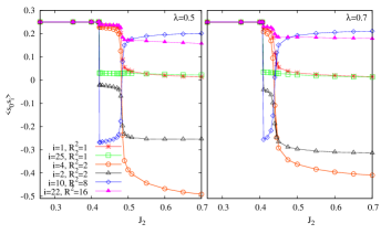
To analyze the GS magnetic ordering we have calculated the spin-spin correlation function $\langle{\bf s}_{0}{\bf s}_{i}\rangle$ as well as a general finite-size order parameterwir04 ; bounce

$$m^{2}=\frac{1}{(N-4)^{2}}\sum_{i,j\notin P}^{N-4}{}|\langle{\bf s}_{i}{\bf s}_{j}\rangle|\,$$ (2)

that adds the total strength of the spin-spin correlation functions. Bearing in mind the strong intra-plaquette correlation functions for $\lambda<1$ we have excluded these correlations in the sum, this way increasing the weight of distant correlation functions.

III.2 Coupled Cluster Method

We first mention that the coupled cluster method (CCM) yields results directly in the thermodynamic limit $N\to\infty$. The CCM has been previously reviewed in several articles (e.g., for the AFMbishop98 ; bishop08 ; xxz ; darradi08 and for the FM $J_{1}$-$J_{2}$ modelrichter10 ; li2012 as well as for dimerized models,krueger00 ; krueger01 ; farnell05 ; farnell09 ) and will not be repeated here in detail. For more general information on the methodology of the CCM, see, e.g., Refs. zeng98, ; bishop98a, ; bishop00, ; bishop04, .

The CCM is a quantum many-body method and is defined by a reference (or model) state $|\Phi\rangle$ and a complete set of mutually commuting many-body creation operators $C_{I}^{+}$. For our model we choose the classical GSs, see Fig. 2, as reference states. It is convenient to perform an appropriate rotation of the local axis of the spins such that in the rotated coordinate frame the reference state is a tensor product of spin down states $|\Phi\rangle=|\downarrow\rangle|\downarrow\rangle|\downarrow\rangle\dots$. The creation operators are then the multispin creation operators $C_{I}^{+}=s_{i}^{+},\,\,s_{i}^{+}s_{j}^{+},\,\,s_{i}^{+}s_{j}^{+}s_{k}^{+},\cdots$ where the indices $i,j,k,\dots$ denote arbitrary lattice sites.

The CCM parameterizations of the ket- and bra- GSs are given by (with $C_{I}^{-}=(C_{I}^{+})^{+}$)

$$|\Psi\rangle=e^{S}|\Phi\rangle,\qquad S=\sum_{I\neq 0}{\cal S}_{I}C_{I}^{+};$$

$$\langle\tilde{\Psi}|=\langle\Phi|\tilde{S}e^{-S},\qquad\tilde{S}=1+\sum_{I\neq 0}\tilde{\cal S}_{I}C_{I}^{-}.$$ (3)

Using $\langle\Phi|C_{I}^{+}=0=C_{I}|\Phi\rangle$ $\forall I\neq 0$, $C_{0}^{+}\equiv 1$, the orthonormality condition $\langle\Phi|C_{I}C_{J}^{+}|\Phi\rangle=\delta_{IJ}$, and the completeness relation $\displaystyle\sum_{I}C_{I}^{+}|\Phi\rangle\langle\Phi|C_{I}=1=|\Phi\rangle\langle\Phi|+\sum_{I\neq 0}C_{I}^{+}|\Phi\rangle\langle\Phi|C_{I}$ we get a set of non-linear and linear equations for the correlation coefficients ${\cal S}_{I}$ and $\tilde{\cal S}_{I}$, respectively. The order parameter (sublattice magnetization) in the rotated coordinate frame is given by

$$M=-\frac{1}{N}\sum_{i}^{N}\langle\tilde{\Psi}|s_{i}^{z}|\Psi\rangle.$$ (4)

In the CCM the only approximation is the truncation of the expansion of the correlation operator $S$ and $\tilde{S}$. We use the well established LSUB$m$ scheme, where all multispin correlations on the lattice with $m$ or fewer contiguous sites are taken into account. The number of these configurations can be reduced using lattice symmetry and conservation laws, but it is increasing very rapidly with $m$. In the highest order of approximation considered here, LSUB10, we have, for example, 180957 configurations for the collinear stripe reference state (CAF) and 219446 for the antiferromagnetic plaquette state (PAF), i.e., finally 180957 or 219446 corresponding coupled non-linear equations which have to be solved numerically.

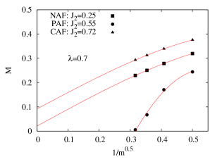
Since the LSUB$m$ approximation scheme becomes exact for $m\to\infty$, we can improve our results by extrapolating the “raw” LSUB$m$ data to $m\to\infty$. There is ample empirical experience regarding how one should extrapolate the magnetic order parameter $M(m)$ for systems with quantum phase transition between magnetically ordered and disordered GS phases. Following Refs. bishop08, ; xxz, ; darradi08, ; richter10, we use $M(m)=b_{0}+b_{1}(1/m)^{1/2}+b_{2}(1/m)^{3/2}$ to extrapolate to $m\to\infty$. As a rulebishop08 ; xxz ; darradi08 ; richter10 the lowest level of approximation, LSUB2, is excluded from extrapolation. For the particular 4-spin plaquette model considered here, we expect LSUB2 to be especially poor, because its cluster size (2 spins) is smaller than the unit cell (4 spins) of the model. Hence, we use LSUB4, LSUB6, LSUB8 and LSUB10 data for the extrapolations.

Figure 3: ED data for the spin-spin correlation functions $\langle{\bf s}_{0}{\bf s}_{i}\rangle$ versus $J_{2}$ (AFM $J_{1}=+1$) for two values of $\lambda$ for the finite lattice of $N=32$ sites. Except the site indeces $0$ and $i$ corresponding to Fig. 1 we also give the square of separation $R^{2}$ of the sites $0$ and $i$. Note that $\langle{\bf s}_{0}{\bf s}_{1}\rangle$ and $\langle{\bf s}_{0}{\bf s}_{4}\rangle$ are intra-plaquette correlation functions, whereas the other ones are inter-plaquette correlation functions.

Figure 4: ED data for the finite-size order parameter $m^{2}/m^{2}_{FM}$ as defined in Eq. (2) versus $J_{2}$ (AFM $J_{1}=+1$) for various values of $\lambda$ for the finite lattice of $N=32$ sites. For convenience $m^{2}$ is scaled by its value for the ferromagnetic state $m^{2}_{FM}=0.25$.

IV Results for the quantum $s=1/2$ model

IV.1 Antiferromagnetic nearest-neighbor exchange $J_{1}$

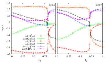
We first consider the AFM case, set $J_{1}=+1$, and start with the discussion of ED data, see Figs. 3 and 4. Corresponding to the three classical phases there are three regimes in the quantum model. The spin-spin correlation functions $\langle{\bf s}_{0}{\bf s}_{i}\rangle$ presented in Fig. 3 for $\lambda=0.5$ and $\lambda=0.7$ are quite strong for small and large $J_{2}$ thus indicating semi-classical magnetic LRO, where the signs of $\langle{\bf s}_{0}{\bf s}_{i}\rangle$ fit to the classical phases NAF and CAF. In an intermediate regime, around $J_{2}=0.5$, the inter-plaquette spin-spin correlations are weak. These three different regimes are also well seen in Fig. 4, where the finite-size order parameter $m^{2}$, see Eq. (2), is shown. In particular, the $m^{2}$ data yield clear evidence for regions with weak magnetic order. The widths of those regions increase drastically with decreasing $\lambda$. Bearing in mind that for $\lambda=1$ the region of magnetic disorder is $0.4\lesssim J_{2}\lesssim 0.6$, see, e.g., Refs. Sir:2006, ; darradi08, ; ortiz, ; fprg, ; ED40, , and balents2011, , our ED data for $N=32$ suggest that there is no semi-classical antiferromagnetic LRO of plaquette type (PAF). Moreover, for small values of $\lambda\lesssim 0.5$ the finite-size order parameter is small in the whole range of $J_{2}$ values indicating the absence of any magnetic LRO.

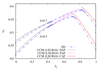
Now we discuss the CCM results ($N\to\infty$). Fig. 5 provides the CCM GS energy per site $e_{0}$ for $\lambda=0.5$ and $\lambda=0.7$ compared with the corresponding ED data. Obviously, the CCM and the ED agree well. To discuss magnetic LRO we consider the CCM-LSUB$m$ magnetic order parameter $M$ (sublattice magnetization) extrapolated to $m\to\infty$, see Eq. (4), that is depicted in Fig. 6. To illustrate the quality of the used extrapolation for the order parameter $M$ of the ‘raw’ LSUB$m$ data to the limit $m\to\infty$ we also show, as an example, corresponding plots for the $\lambda=0.7$ in Fig. 7. It is obvious that the LSUB$m$ data are well fitted by the applied extrapolation function.

Figure 5: CCM LSUB10 data for the GS energy $e_{0}$ (AFM $J_{1}=+1$) for $\lambda=0.5$ and $\lambda=0.7$ compared with corresponding ED data ($N=32$). The CCM results correspond to the NAF reference state (small $J_{2}$), the PAF reference state (intermediate $J_{2}$), and the CAF reference state (large $J_{2}$).

Figure 6: Extrapolated CCM data for the magnetic order parameter (sublattice magnetization) $M$ for the AFM case ($J_{1}=+1$) and for various values of $\lambda$. The CCM reference state is the NAF state (left hand side, small $J_{2}$) and the CAF state (right hand side, large $J_{2}$). The extrapolated CCM data are obtained using LSUB$m$ with $m=4,6,8,10$ and the extrapolation rule $M(m)=b_{0}+b_{1}(1/m)^{1/2}+b_{2}(1/m)^{3/2}$.

Figure 7: Illustration of the extrapolation (solid lines) of the CCM-LSUB$m$ data (symbols) for the magnetic order parameter $M$ for $\lambda=0.7$, $J_{1}=+1$ and specific values of $J_{2}$ corresponding to the NAF, PAF, CAF reference states. For the extrapolations to $m\to\infty$ according to $M(m)=b_{0}+b_{1}(1/m)^{1/2}+b_{2}(1/m)^{3/2}$ we have used LSUB$m$ data for $m=4,6,8,10$.

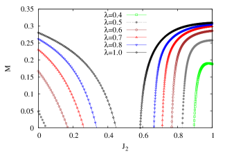
First we notice that the extrapolated order parameter using the PAF reference state for all relevant parameter sets of $\lambda$ and $J_{2}$ vanishes (see also Fig. 7), i.e., there is no PAF magnetic LRO in the quantum model. This finding is in agreement with the ED data for $m^{2}$ discussed above (and see again Fig. 4). The range of stability of the semi-classical NAF and CAF phases is visible in Fig. 6. We define the quantum critical points $J_{2}^{c1}(\lambda)$ and $J_{2}^{c2}(\lambda)$ as those points, where the extrapolated CCM magnetic order parameter $M$ vanishes. For $\lambda=1$ (uniform model) we find $J_{2}^{c1}=0.447J_{1}$ and $J_{2}^{c2}=0.586J_{1}$ which is in agreement with previous CCM predictions.bishop08 ; xxz ; darradi08 As expected, with decreasing of $\lambda$ the region of $J_{2}$ values without magnetic LRO increases, see Fig. 6. Collecting the data for the quantum critical points $J_{2}^{c1}$ and $J_{2}^{c2}$ for various $\lambda$ we get the GS phase diagram of the quantum model as shown Fig. 8. Our phase diagram is in good agreement with the only available corresponding one of Ref. singh99, . Hence, one can argue that the phase diagram is basically correct.

Concerning the order of the quantum phase transitions at $J_{2}^{c1}$ and $J_{2}^{c2}$ our data are in favor of a continuous transition at $J_{2}^{c1}$ and a first-order transition at $J_{2}^{c2}$ as it is was discussed for the uniform model.schulz ; singh99 ; sushkov01 ; ED40 The scenario of a first-order transition between the QPM and the CAF phases is supported by (i) the kink-like behavior in $e_{0}$, see Fig. 5, (ii) the steep fall in the CCM order parameter $M$ near $J_{2}^{c2}$, see Fig. 6, and (iii) the jump-like behavior of the spin-spin correlations functions, see Fig. 3, and of the finite-size order parameter, see Fig. 4.

Figure 8: The CCM GS phase diagram of the model (1) for the AFM case ($J_{1}=+1$). NAF denotes the semi-classical phase with Néel LRO, CAF the semi-classical phase with collinear striped antiferromagnetic LRO, and QPM the magnetically disordered quantum paramagnetic phase. For comparison we also show the classical transition lines (thin dashed lines), cf. Fig. 2.

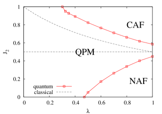
For the unfrustrated case $J_{2}=0$ we can compare our result $\lambda_{c}=0.47$ (and see Fig. 8) for the critical $\lambda$ where the NAF LRO breaks down with several previous results, namely $\lambda_{c}=0.555$ (Ising series expansionsingh99 ) $\lambda_{c}=0.6$ (exact diagonalizationvoigt02 ) $\lambda_{c}=0.5485$ (QMCfabricio08 ; wenzel09 ), $\lambda_{c}=0.5491\dots 0.5513$ (contractor renormalization expansionfabricio08 ), and $\lambda_{c}=0.4822$ (real space renormalization group approachfledderjohann09 ). Likely, the QMC result is most accurate. Our result is in reasonable agreement with that result, but slightly overestimates the stability region of NAF LRO.

Let us briefly discuss another limit of the model, namely the limit of large $J_{2}$. As discussed above in that limit the system splits into two interpenetrating square-lattice Heisenberg antiferromagnets (where $J_{2}$ plays the role of the AFM NN bond), which are Néel-ordered for $\lambda=1$. Hovewer, for $\lambda<1$ each of the two interpenetrating square lattices carries now a staggered arrangement of $J_{2}$ and $\lambda J_{2}$ bonds, which corresponds precisely to the so-called $J$-$J^{\prime}$ model discussed in Refs. singh88, ; ivanov96, ; krueger00, ; wenzel08, ; wenzel09, ; vidal09, . The QMC estimate of the critical $\lambda$ is $\lambda_{c}=0.397$, see Ref. wenzel08, . For $J_{2}=1$ we find from our CCM data a critical value of $\lambda_{c}=0.301$ (see Fig. 8). Increasing of $J_{2}$ beyond $J_{2}=1$ (not shown in Fig. 8) yields a steep increase of the critical line as already indicated by the last two data points near $J_{2}=1$ in Fig. 8. In the limit of large $J_{2}$ the critical $\lambda_{c}$ is even smaller as for $J_{2}=1$. For example at $J_{2}=5$ we obtain $\lambda_{c}=0.375$ that is in good agreement with the QMC result for the critical $\lambda_{c}$ of the $J$-$J^{\prime}$ model. Note that our value of $\lambda_{c}$ deviates from an early CCM result $\lambda_{c}=0.316$.krueger00 The difference is related to the fact that we use here (i) a higher approximation level (LSUB10) and (ii) an improved extrapolation in comparison with Ref. krueger00, .

IV.2 Ferromagnetic nearest-neighbor exchange $J_{1}$

Figure 9: ED data for the spin-spin correlation functions $\langle{\bf s}_{0}{\bf s}_{i}\rangle$ versus $J_{2}$ (FM $J_{1}=-1$) for two values of $\lambda$ for the finite lattice of $N=32$ sites. Except the site indeces $0$ and $i$ corresponding to Fig. 1 we also give the square of separation $R^{2}$ of the sites $0$ and $i$. Note that $\langle{\bf s}_{0}{\bf s}_{1}\rangle$ and $\langle{\bf s}_{0}{\bf s}_{4}\rangle$ are intra-plaquette correlation functions, whereas the other ones are inter-plaquette correlation functions.

Figure 10: ED data for the finite-size order parameter $m^{2}/m^{2}_{FM}$ as defined in Eq. (2) versus $J_{2}$ (FM $J_{1}=-1$) for various values of $\lambda$ for the finite lattice of $N=32$ sites. For convenience $m^{2}$ is scaled by its value for the ferromagnetic state $m^{2}_{FM}=0.25$.

Figure 11: CCM-LSUB10 (thick lines) and LSUB6 data (thin lines) for the GS energy $e_{0}$ ($J_{1}=-1$) for $\lambda=0.5$ and $\lambda=0.7$ compared with corresponding ED data ($N=32$). The CCM results correspond to the PFM reference state (intermediate $J_{2}$) and the CAF reference state (large $J_{2}$). The black solid line is the exact FM GS energy.

We now consider the FM case and set $J_{1}=-1$. Although, the classical phase diagrams for $J_{1}=-1$ and $J_{1}=+1$ are identical, see Fig. 2, we know from the uniform model (i.e., $\lambda=1$) that the phase diagrams in the quantum case $s=1/2$ are basically different.shannon04 ; shannon06 ; sindz07 ; schmidt07 ; schmidt07_2 ; sousa ; shannon09 ; sindz09 ; haertel10 ; richter10 ; momoi2011 ; cabra2011 In particular, it was found for $J_{1}=-1$ that the region of semi-classical CAF LRO extends up to much smaller values of $J_{2}$ compared with the case of $J_{1}=+1$.richter10 ; cabra2011 Hence, we expect also for $\lambda<1$ basic differences between $J_{1}=+1$ and $J_{1}=-1$.

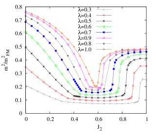
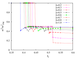
We start again with ED results for the spin-spin correlation functions $\langle{\bf s}_{0}{\bf s}_{i}\rangle$, see Fig. 9, and the finite-size order parameter $m^{2}$ defined in Eq. (2), see Fig. 10. The three classical phases lead again to three different regimes in the quantum model. The trivial FM state at small $J_{2}$ is of course also present in the quantum model. It gives way at $J_{2}^{c1}(\lambda)$ for an intermediate singlet state. This transition at $J_{2}^{c1}$ is clearly seen by jumps in $\langle{\bf s}_{0}{\bf s}_{i}\rangle$ and $m^{2}$. $J_{2}^{c1}$ is smaller than the classical value $J_{2,clas}^{c1}=0.5$, and it depends on $\lambda$ for the quantum model. Moreover, there is a second jump-like behavior of the spin-spin correlation functions indicating the transition from the intermediate regime to the CAF regime. We can use the positions of these jumps to extract the transition points $J_{2}^{c1}$ and $J_{2}^{c2}$ between the regimes from our ED calculations, see the discussion of Fig. 12 given below.

The main difference in comparison to the AFM model ($J_{1}=+1$) concerns the intermediate regime. From Fig. 9 it is evident that the inter-plaquette correlation functions $\langle{\bf s}_{0}{\bf s}_{10}\rangle$ and $\langle{\bf s}_{0}{\bf s}_{22}\rangle$, see Fig. 1, are not small. Hence, the intermediate phase might be long-range ordered for FM $J_{1}$. Indeed, in the finite-size order parameter $m^{2}$ shown in Fig. 10 an intermediate regime is clearly visible for $\lambda\lesssim 0.5$, where the finite-size order parameter $m^{2}$ in this regime is much larger than that for $J_{1}=+1$ (cf. Fig. 4). The possible appearance of magnetic LRO can be understood on the basis of the classical PFM state (see also Sec. II): The elementary unit is the 4-spin-plaquette (with strong bonds). Due to the strong FM intra-plaquette bond $J_{1}$ the plaquette carries an effective block (composite) spin $s=2$. These block spins interact via $\lambda J_{2}$ and form effectively two interpenetrating square-lattice $s=2$ Heisenberg antiferromagnets.

Figure 12: GS phase diagram of the plaquette model of Eq. (1) for the FM case ($J_{1}=-1$). The transition lines between the FM and the PFM phases as well as the PFM and the CAF/QPM phases are obtained by (i) ED by using the jumps in the ED data (black lines), see Figs. 9 and 10, and (ii) by CCM from the intersection points between the GS energies using various reference states for the CCM calculation (blue lines), see text. The transition lines between the CAF and the QPM phase (red line) correspond to those parameter values ($\lambda,J_{2}$), where the extrapolated CCM order parameter vanishes (and see Fig. 14). For comparison we also show the classical transition lines (magenta line), cf. Fig. 2.

Figure 13: CCM magnetic order parameter $M$ for the FM case ($J_{1}=-1$) versus $J_{2}$ using the PFM and the CAF states as CCM reference states for $\lambda=0.5$ and $\lambda=0.7$. The extrapolated CCM results are obtained using LSUB$m$ with $m=4,6,8,10$ and the extrapolation rule $M(m)=b_{0}+b_{1}(1/m)^{1/2}+b_{2}(1/m)^{3/2}$.

Figure 14: Magnetic order parameter $M$ for the FM case ($J_{1}=-1$) versus $\lambda$ for $J_{2}=1.0$ (filled triangles), $0.7$ (circles) and $0.5$ (lines) using the PFM and the CAF states as CCM reference states. The extrapolated CCM results are obtained using LSUB$m$ with $m=4,6,8,10$ and the extrapolation rule $M(m)=b_{0}+b_{1}(1/m)^{1/2}+b_{2}(1/m)^{3/2}$.

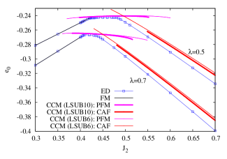
Now we pass to the CCM results ($N\to\infty$). Fig. 11 provides the CCM GS energy per site $e_{0}$ for $\lambda=0.5$ and $\lambda=0.7$ in LSUB6 and LSUB10 approximation compared with the corresponding ED data. The agreement between the CCM and the ED is good. The three regimes, FM, PFM, and CAF, are clearly seen in the energy data. For the CCM estimate for the transition point $J_{2}^{c1}$ between the FM state and the PFM regime we use the intersection points between the FM energy and the CCM-LSUB10 as well as the LSUB6 energy calculated with the PFM reference state. Both results for $J_{2}^{c1}$ almost coincide, see Fig. 12. Moreover, we find an excellent agreement between the ED and CCM results for $J_{2}^{c1}$. Concerning the order of the phase transition at $J_{2}^{c1}$ we have clear evidence for a first-order transition as indicated by (i) the jump-like behavior of the spin-spin correlations functions, see Fig. 9, and of the finite-size order parameter, see Fig. 10, (ii) the kink-like behavior in $e_{0}$, see Fig. 11, and (iii) the jump in the CCM order parameter $M$ at $J_{2}^{c1}$, see Fig. 13.

To determine the transition point $J_{2}^{c2}$ between the PFM and the CAF regimes we are faced with the problem that near this transition no CCM-LSUB10 solutions for the CAF reference state could be found. This observation, that for high orders of CCM approximation in the vicinity of an intersection point of two CCM energy curves belonging to two different GS phases no solution of the large set of coupled nonlinear ket equations can be obtained, is often found when dealing with strongly frustrated systems, see, e.g., Refs. Schm:2006, and richter10, . However, from Fig. 11 it is obvious that the parameter range, where solutions for lower levels $m$ of LSUB$m$ approximations can be found, is much larger than for LSUB10. Moreover, the LSUB$m$ data for $e_{0}$ for various $m$ are very close to each other. Hence, we can use the intersection points for lower levels of CCM-LSUB$m$ approximation to determine the second transition point $J_{2}^{c2}$. Thus, we find intersection points for LSUB8, LSUB6, and LSUB4 for $\lambda\geq 0.7$, $\lambda\geq 0.5$, and $\lambda\geq 0.25$, respectively. In addition, we can also take benefit from the almost straight behavior of $e_{0}(J_{2})$ curves, see Fig. 11, which allows a reliable extrapolation of $e_{0}(J_{2})$ until a hypothetical intersection point, cf. also Refs. richter10, and cabra2011, . This gives finally various sets of $J_{2}^{c2}(\lambda)$ data, which, however, agree well with each other, cf. Fig. 12. Only for $\lambda\lesssim 0.3$ a slight difference is visible. Nevertheless, it is necessary to mention that the CCM estimate for $J_{2}^{c2}(\lambda)$ becomes less reliable for smaller values of $\lambda$ due to the increasing distance between the hypothetical intersection points and the last data points for which LSUB$m$ solutions for the CAF reference state could be found.

Figure 15: Illustration of the extrapolation (solid lines) of the CCM-LSUB$m$ data (symbols) for the magnetic order parameter $M$ for $\lambda=0.5$, $J_{1}=-1$ and specific values of $J_{2}$ corresponding to the CAF and PFM reference states. For the extrapolations to $m\to\infty$ according to $M(m)=b_{0}+b_{1}(1/m)^{1/2}+b_{2}(1/m)^{3/2}$ we have used LSUB$m$ data for $m=4,6,8,10$.

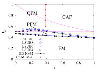
The results for $J_{2}^{c1}(\lambda)$and $J_{2}^{c2}(\lambda)$ obtained by ED and CCM are collected in the phase diagram presented in Fig. 12. It is obvious that both, ED and CCM, yield very similar values for $J_{2}^{c1}$ and $J_{2}^{c2}$.

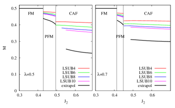
The question about magnetic LRO in the various regimes we address next by analyzing the CCM magnetic order parameter $M$ for the PFM and CAF regimes. (Remember that in the trivial FM phase we have always $M=1/2$.) In Fig. 13 we show $M$ versus $J_{2}$ for $\lambda=0.5$ and $\lambda=0.7$. Obviously, the order parameter in the PFM regime is non-zero and even larger than in the CAF regime. This observation is in agreement with our ED results, cf. Fig.  10, and can be related to the effective block-spin $s=2$ model discussed above. The order parameter in the CAF is only weakly dependent on $J_{2}$, but its magnitude depends on $\lambda$. As discussed above we do not get CAF CCM solutions for LSUB$m$ for higher values of $m$ near the transition to the PFM phase. Nevertheless, the curves presented in Fig. 13 indicate that there is likely a direct first-order transition at $J_{2}^{c2}$ between semi-classical phases with PFM and CAF magnetic LRO for $\lambda\gtrsim 0.4$.

Next we fix $J_{2}$ and consider the behavior of the order parameter $M$ in dependence on $\lambda$, see Fig. 14. For values of $J_{2}\gtrsim 0.55$ the PFM regime is not relevant. As explained in Sec. IV.1 in the limit of large $J_{2}$ our plaquette model corresponds to the $J$-$J^{\prime}$ model, where at $\lambda=\lambda_{c}=0.397$ (QMC result, see Ref. wenzel08, ) a second-order transition to a QPM phase takes place. This behavior is clearly seen in our CCM data for $M(\lambda)$ for $J_{2}=1.0$ and $J_{2}=0.7$ shown in Fig. 14. We find that for $J_{2}\gtrsim 0.6$ the extrapolated CCM order parameter $M$ vanishes continuously at a critical value $\lambda=\lambda_{c}(J_{2})$ defining a second-order transition between a semi-classical phase with CAF magnetic LRO and the QPM phase, that is depicted as a red line in Fig. 12. Interestingly, $\lambda_{c}$ practically does not depend on $J_{2}$ and we have $\lambda_{c}\approx 0.383$ for $0.6\lesssim J_{2}\leq 1$. This value is close to the QMC valuewenzel08 $\lambda_{c}=0.397$ valid for $J_{2}\to\infty$ and also to $\lambda_{c}=0.375$ obtained for the AFM model ($J_{1}=+1$) for $J_{2}=5$, see Sec. IV.1.

For $J_{2}=0.5$ the situation is different, since both, the PFM and CAF regimes, play a role. For $\lambda<0.494$ we are inside the PFM regime. Obviously, the PFM order parameter is large and the variation with $\lambda$ is weak. Within the CAF regime we are again faced with the problem that the CAF LSUB$m$ solutions for higher $m$ terminate before meeting the corresponding PFM LSUB$m$ solutions. Hence, the critical line $\lambda_{c}(J_{2})$ (red vertical line in Fig. 12) terminates before meeting the transition line $J_{2}^{c2}(\lambda)$, and we cannot give a secure statement on the continuation of the critical line $\lambda_{c}(J_{2})$ towards lower values of $J_{2}$.

Finally, we illustrate the quality of the used extrapolation for the order parameter $M$ of the ‘raw’ LSUB$m$ data to the limit $m\to\infty$ for $\lambda=0.7$ in Fig. 15. It is obvious that the LSUB$m$ data are well fitted by the applied extrapolation function.

Let us briefly discuss the relation of our results to the schematic phase diagram previously presented in Ref. ueda07, . As stated in Ref. ueda07, the approximations used there (bond-operator mean-field theory as well as a second-order perturbation theory in $\lambda$) may be not reliable for large $\lambda\sim 1$ and large $J_{2}\sim 1$. The main features of our phase diagram agree well with those presented in Ref. ueda07, . For $\lambda\to 0$ we obtain the same transition point $J_{2}^{c2}=0.5$ between the QPM and the PFM phases. However, for $\lambda\sim 1$ and $J_{2}\sim 1$ some differences appear. For instance, we do not find a nematic phase for $\lambda\lesssim 1$, as it was discussed in Ref. ueda07, . Note that the absence of the nematic phase is in agreement with the recent findings for the uniform model, i.e. at $\lambda=1$.richter10 ; cabra2011 Moreover, the second-order transition between the QPM and CAF phases for large $J_{2}$ is found in Ref. ueda07, at $\lambda\approx 0.5$, but it should be at $\lambda\approx 0.4$.

V Summary

Inspired by a recent investigation of a frustrated two-dimensional Heisenberg model proposed to describe the magnetic properties of (CuCl)LaNb₂O₇, see Refs. kageyama05, and ueda07, , we investigate the GS phase diagram of the spin-$1/2$ $J_{1}$-$J_{2}$ Heisenberg model on the square lattice with plaquette structure. The 4-site plaquettes carrying the (strong) intra-plaquette bonds $J_{1}$ and $J_{2}$ are coupled to each other by (weaker) inter-plaquette bonds $\lambda J_{1}$ and $\lambda J_{2}$, $0\leq\lambda\leq 1$. The parameter $\lambda$ can also be thought of modeling a distortion of the underlying square lattice.

We consider AFM ($J_{1}>0$) as well as FM nearest-neighbor exchange coupling ($J_{1}<0$). Except the phases with magnetic LRO (FM, Néel, and collinear striped AFM) and the non-magnetic quantum paramagnetic phase known from the standard spin-$1/2$ $J_{1}$-$J_{2}$ model we find for FM $J_{1}$ a new plaquette phase showing antiferromagnetic long-range of $s=2$ block spins associated with 4-spin plaquettes. For the AFM model ($J_{1}>0$) the region of the quantum paramagnetic phase is significantly increased for $\lambda<1$ compared to the standard model, thus increasing the prospects of finding a magnetically disordered low-temperature phase in real magnetic materials, where the exchange pattern may deviate from the standard $J_{1}$-$J_{2}$ model, see, e.g., Refs. rosner2010, ; volkova2010, and janson2010, .

References

- (1) P. Chandra and B. Doucot, Phys. Rev. B 38, 9335 (1988).
- (2) E. Dagotto and A. Moreo, Phys. Rev. Lett. 63, 2148 (1989).
- (3) H.J. Schulz and T.A.L. Ziman, Europhys. Lett. 18, 355 (1992); H.J. Schulz, T.A.L. Ziman, and D. Poilblanc, J. Phys. I 6, 675 (1996).
- (4) J. Richter, Phys. Rev. B 47, 5794 (1993).
- (5) J. Richter, N.B. Ivanov, and K. Retzlaff, Europhys. Lett. 25, 545 (1994).
- (6) M.E. Zhitomirsky and K. Ueda Phys. Rev. B 54, 9007 (1996).
- (7) A. E. Trumper, L. O. Manuel, C. J. Gazza, and H. A. Ceccatto, Phys. Rev. Lett. 78, 2216 (1997).
- (8) R.F. Bishop, D.J.J. Farnell, and J.B. Parkinson, Phys. Rev. B 58, 6394 (1998).
- (9) R. R. P. Singh, Z. Weihong, C. J. Hamer, and J. Oitmaa, Phys. Rev. B 60, 7278 (1999).
- (10) L. Capriotti, F. Becca, A. Parola, and S. Sorella, Phys. Rev. Lett. 87, 097201 (2001).
- (11) O. P. Sushkov, J. Oitmaa, and Z. Weihong, Phys. Rev. B 63, 104420 (2001).
- (12) J. Sirker, Z. Weihong, O. P. Sushkov, and J. Oitmaa, Phys. Rev. B 73, 184420 (2006).
- (13) D. Schmalfuß, R. Darradi, J. Richter, J. Schulenburg, and D. Ihle, Phys. Rev. Lett. 97, 157201 (2006).
- (14) J.R. Viana and J.R. de Sousa, Phys. Rev. B 75, 052403 (2007).
- (15) R.F. Bishop, P.H.Y. Li, R. Darradi, and J. Richter, J. Phys.: Condens. Matter 20, 255251 (2008).
- (16) R.F. Bishop, P.H.Y. Li, R. Darradi, J. Schulenburg and J. Richter, Phys. Rev. B 78, 054412 (2008).
- (17) R. Darradi, O. Derzhko, R. Zinke, J. Schulenburg, S. E. Krüger, and J. Richter, Phys. Rev. B 78, 214415 (2008).
- (18) L. Isaev, G. Ortiz, and J. Dukelsky, Phys. Rev. B 79, 024409 (2009).
- (19) T. Pardini and R.R.P. Singh, Phys. Rev. B 79, 094413 (2009).
- (20) V. Murg, F. Verstraete, and J. I. Cirac, Phys. Rev. B 79, 195119 (2009).
- (21) J. Richter and J. Schulenburg, Eur. Phys. J. B 73, 117 (2010).
- (22) J. Reuther and P. Wölfle, Phys. Rev. B 81, 144410 (2010).
- (23) A. Sfondrini, J. Cerrillo, N. Schuch, and J. I. Cirac, Phys. Rev. B 81, 214426 (2010).
- (24) H.-C. Jiang, H. Yao, L. Balents, arXiv:1112.2241 (2011).
- (25) L. Wang, Z.-C. Gu, X.-G. Wen, F. Verstraete, arXiv:1112.3331 (2011).
- (26) E. E. Kaul, H. Rosner, N. Shannon, R.V. Shpanchenko, and C. Geibel, J. Magn. Magn. Mater. 272-276(II), 922 (2004).
- (27) M. Skoulatos, J.P. Goff, N. Shannon, E.E. Kaul, C. Geibel, A.P. Murani, M. Enderle, and A.R. Wildes, J. Magn. Magn. Mater. 310, 1257 (2007).
- (28) P. Carretta, M. Filibian, R. Nath, C. Geibel, and P. J. C. King, Phys. Rev. B 79, 224432 (2009).
- (29) M. Skoulatos, J.P. Goff, C. Geibel, E.E. Kaul, R. Nath, N. Shannon, B. Schmidt, A.P. Murani, P.P. Deen, M. Enderle, and A.R. Wildes, Europhys. Lett. 88, 57005 (2009).
- (30) R. Nath, Y. Furukawa, F. Borsa, E. E. Kaul, M. Baenitz, C. Geibel, and D. C. Johnston, Phys. Rev. B 80, 214430 (2009).
- (31) A.A. Tsirlin and H. Rosner, Phys. Rev. B 79, 214417 (2009).
- (32) A.A. Tsirlin, B. Schmidt, Y. Skourski, R. Nath, C. Geibel, and H. Rosner, Phys. Rev. B 80, 132407 (2009).
- (33) L. Bossoni, P. Carretta, R. Nath, M. Moscardini, M. Baenitz, and C. Geibel, Phys. Rev. B 83, 014412 (2011).
- (34) R. Nath, A.A. Tsirlin, H. Rosner, and C. Geibel, Phys. Rev. B 78 064422 (2008).
- (35) N. Shannon, B. Schmidt, K. Penc, and P. Thalmeier, Eur. Phys. J. B 38, 599 (2004).
- (36) N. Shannon, T. Momoi, and P. Sindzingre, Phys. Rev. Lett. 96, 027213 (2006).
- (37) P. Sindzingre, N. Shannon and T. Momoi, J. Magn. Magn. Mat. 310, 1340 (2007).
- (38) B. Schmidt, N. Shannon, and P. Thalmeier, J. Phys.: Condens. Matter 19, 145211 (2007).
- (39) B. Schmidt, N. Shannon, and P. Thalmeier, J. Magn. Magn. Mater. 310, 1231 (2007).
- (40) P. Sindzingre, L. Seabra, N. Shannon, and T. Momoi, J. Phys.: Conf. Series 145, 012048 (2009).
- (41) P. Sindzingre, N. Shannon, and T. Momoi, J. Phys.: Conf. Series 200, 022058 (2010).
- (42) M. Härtel, J. Richter, D. Ihle, and S.-L. Drechsler, Phys. Rev. B 81, 174421 (2010).
- (43) J. Richter, R. Darradi, J. Schulenburg, D. J. J. Farnell, and H. Rosner, Phys. Rev. B 81, 174429 (2010).
- (44) R. Shindou, S. Yunoki, and T. Momoi, Phys. Rev. B 84, 134414 (2011).
- (45) H. Feldner, D. C. Cabra, and G. L. Rossini, Phys. Rev. B 84, 214406 (2011).
- (46) H.-J. Schmidt, J. Phys. A 38, 2123 (2005).
- (47) A. Voigt, Comp. Phys. Comm. 146, 125 (2002).
- (48) H.T. Ueda and K. Totsuka, Phys. Rev. B 76, 214428 (2007).
- (49) A. F. Albuquerque, M. Troyer, and J. Oitmaa, Phys. Rev. B 78, 132402 (2008).
- (50) S. Wenzel, L. Bogacz, and W. Janke, Phys. Rev. Lett. 101, 127202 (2008).
- (51) S. Wenzel and W. Janke, Phys. Rev. B 79, 014410 (2009).
- (52) A. Fledderjohann, A. Klümper, and K.-H. Mütter, Eur. Phys. J. B. 72, 551 (2009); Eur. Phys. J. B. 72, 559 (2009).
- (53) A.A. Tsirlin, R. Nath, A.M. Abakumov, R.V. Shpanchenko, C. Geibel, and H. Rosner, Phys. Rev. B 81, 174424 (2010).
- (54) H. Kageyama, T. Kitano, N. Oba, M. Nishi, S. Nagai, K. Hirota, L. Viciu, J. B. Wiley, J. Yasuda, Y. Baba, Y. Ajiro, and K. Yoshimura, J. Phys. Soc. Jpn. 74, 1702 (2005).
- (55) A. A. Tsirlin, A. M. Abakumov, G. Van Tendeloo, and H. Rosner, Phys. Rev. B 82, 054107 (2010), A.A. Tsirlin and H. Rosner, Phys. Rev. B 82, 060409 (2010).
- (56) http://www-e.uni-magdeburg.de/jschulen/spin/.
- (57) J. Richter, J. Schulenburg and A. Honecker, in Quantum Magnetism, eds U. Schollwöck, J. Richter, D.J.J. Farnell, and R.F. Bishop, Lecture Notes in Physics 645 (Springer-Verlag, Berlin, 2004), p. 85.
- (58) D.J.J. Farnell, R. Darradi, R. Schmidt, and J. Richter, Phys. Rev. B 84, 104406 (2011).
- (59) P.H.Y. Li, R.F. Bishop, D.J.J. Farnell, J. Richter, and C. E. Campbell, Phys. Rev. B 85, 085115 (2012).
- (60) S. E. Krüger, J. Richter, J. Schulenburg, D. J. J. Farnell, and R. F. Bishop, Phys. Rev. B 61, 14607 (2000).
- (61) S. E. Krüger and J. Richter, Phys. Rev. B 64, 024433 (2001).
- (62) D.J.J. Farnell, J. Schulenburg, J. Richter, and K.A. Gernoth, Phys. Rev. B 72, 172408 (2005)
- (63) D.J.J. Farnell, J. Richter; R. Zinke; R.F. Bishop, J. Stat. Phys., 135, 175 (2009)
- (64) C. Zeng, D. J. J. Farnell, and R. F. Bishop, J. Stat. Phys. 90, 327 (1998).
- (65) R. F. Bishop, in Microscopic Quantum Many-Body Theories and Their Applications, edited by J. Navarro and A. Polls, Lecture Notes in Physics 510 (Springer-Verlag, Berlin, 1998), p.1.
- (66) R. F. Bishop, D. J. J. Farnell, S. E. Krüger, J. B. Parkinson, J. Richter, and C. Zeng, J. Phys.: Condens. Matter 12, 6887 (2000).
- (67) D. J. J. Farnell and R. F. Bishop, in Quantum Magnetism, Lecture Notes in Physics Vol. 645, edited by U. Schollwöck, J. Richter, D. J. J. Farnell, and R. F. Bishop (Springer, Berlin, 2004), p. 307.
- (68) R.R.P. Singh and M.P. Gelfand, Phys. Rev. Lett. 61, 2484 (1988).
- (69) N.B. Ivanov, S.E. Krüger, and J. Richter, Phys. Rev. B 53, 2633 (1996).
- (70) B. Bauer, G. Vidal, and M. Troyer, J. Stat. Mech. P09006 (2009).
- (71) O. Volkova, I. Morozov, V. Shutov, E. Lapsheva, P. Sindzingre, O. Cepas, M. Yehia, V. Kataev, R. Klingeler, B. Büchner, and A. Vasiliev, Phys. Rev. B 82, 054413 (2010).
- (72) O. Janson, A. A. Tsirlin, and H. Rosner, Phys. Rev. B 82, 184410 (2010).