Holographic Cosmological Backgrounds, Wilson Loop (De)confinement and Dilaton Singularities

Abstract

We review a construction of holographic geometries dual to $\mathcal{N}=4$ SYM theory on a Friedmann-Robertson-Walker background and in the presence or absence of a gluon condensate and instanton density. We find the most general solution with arbitrary scale factor and show that it is diffeomorphic to topological black holes. We introduce a time-dependent boundary cosmological constant $\lambda(t)$ and show energy-momentum conservation in this background. For constant $\lambda$, the deconfinement properties of the temporal Wilson loop are analysed. In most cases the Wilson loop confines throughout cosmological evolution. However, there is an exceptional case which shows a transition from deconfinement at early times to confinement at late times. We classify the presence or absence of horizons, with important implications for the Wilson loop.

1 Background and Holographic Stress Energy Tensor

In AdS/CFT, the holographically defined theory is only sensitive to the conformal class of the boundary metric, not the metric itself. It is hence possible to put any holographically defined flat space field theory on $dS_{4}$ or $AdS_{4}$ via an appropriate boundary conformal transformation, amounting to particular bulk diffeomorphisms. The same holds for any metric of Friedmann-Robertson-Walker (FRW) type,

$$ds_{(0)}^{2}=-dt^{2}+a_{0}^{2}(t)d\Omega_{k}^{2}\,.$$ (1)

It is hence conceivable that holographic duals for field theories living on an FRW universe can be constructed in such a way. Such a construction from 5D Einstein-Hilbert theory has been put forward in [3], describing a universal sector of any holographic theory with a stress-energy tensor. In the following we review such a construction [1] based on the background of [5]. This $\mathcal{N}=2$ supersymmetric background describes $\mathcal{N}=4$ SYM theory in a vacuum of constant (anti) self-dual instanton density, and is known to lead to Wilson loop confinement. We will first review the derivation of the cosmological background presented in [1], and then show its diffeomorphism equivalence to the static geometry of [5]. In this course we will find a more general class of solutions including the one of [1], clarify issues regarding the implications of holographic stress energy tensor conservation, comment on the meaning of $a_{0}(t)$ and the boundary cosmological constant $\lambda(t)$ from a bulk perspective, and classify the horizons appearing in the cosmological solution. In sec. 2 we then classify the (de)confinement properties of the Wilson loop in this background, and compare to the AdS-Schwarzschild case.

Ten-dimensional type IIB supergravity truncates to the metric $g$, dilaton $\Phi$, axion $\chi$ and five form $F_{(5)}$,

$$S={1\over 2\kappa^{2}}\int d^{10}x\sqrt{-g}\left(R-{1\over 2}(\partial\Phi)^{2}+{1\over 2}e^{2\Phi}(\partial\chi)^{2}-{1\over 4\cdot 5!}F_{(5)}^{2}\right)\,.$$ (2)

The other IIB fields are consistently set to zero, and $\chi$ is Wick rotated [6]. Under the Freund-Rubin ansatz $F_{\mu_{1}\cdots\mu_{5}}=-\sqrt{\Lambda}/2~{}\epsilon_{\mu_{1}\cdots\mu_{5}}$ [8, 5] and $\mathcal{M}_{10}=\mathcal{M}_{5}\times S^{5}$, the action reduces to

$$S={1\over 2\kappa_{5}^{2}}\int d^{5}x\sqrt{-g}\left(R+3\Lambda-{1\over 2}(\partial\Phi)^{2}+{1\over 2}e^{2\Phi}(\partial\chi)^{2}\right)\,.$$ (3)

Its equations of motion have an $\mathcal{N}=2$ supersymmetric solution if [6, 8]

$$\chi=-e^{-\Phi}+\chi_{0}\ ,$$ (4)

for some constant $\chi_{0}$. Under this Ansatz the metric decouples from the axion-dilaton,

$$R_{MN} = -\Lambda g_{MN}\,,\quad 0=\partial_{M}\left(\sqrt{-g}g^{MN}\partial_{N}e^{\Phi}\right)\,.$$ (5)

In [1] we followed [2] and examined time-dependent solutions of the form

$$ds^{2}_{\rm E}=-n^{2}(t,y)dt^{2}+a(t,y)^{2}d\Omega_{k}^{2}+dy^{2}\,,\quad i,j=1,\dots,3.$$ (6)

The $tt$ and $yy$ components of (5) become [2]

$$\left({\dot{a}\over na}\right)^{2}+{k\over a^{2}}=-{\Lambda\over 4}+\left({a^{\prime}\over a}\right)^{2}+{C\over a^{4}}\,,\quad\dot{a}=\partial a/\partial t\,,\quad a^{\prime}=\partial a/\partial y\,.$$ (7)

This first order equation comes from integrating Einstein’s equations (see [2, 9] for details). The dark radiation constant $C$ appears in (7) as a radiation term ${C\over a^{4}}$ [9, 7]. The remaining $ty$ component reads

$$0=\frac{n^{\prime}}{n}\frac{\dot{a}}{a}-\frac{\dot{a}^{\prime}}{a}\quad\Rightarrow\quad n(t,y)={\dot{a}(t,y)\over\eta(t)}\,.$$ (8)

General Solution and Time Independence of $\lambda$ The most general solution of (7) and (8) depends onn two arbitrary functions of time, $\theta(t)$ and $\eta(t)$,

$$a^{2}=\frac{C+\Lambda^{-1}\left(\Lambda\theta(t)e^{\sqrt{\Lambda}y}-k-\eta^{2}(t)\right)^{2}}{\Lambda\theta(t)e^{\sqrt{\Lambda}y}},\quad n=\frac{\dot{a}}{\eta(t)}\,.$$ (9)

With $\sqrt{\Lambda}=2/R$, $\exp(\sqrt{\Lambda}y)=(r/R)^{2}$, $\theta(t)=a_{0}^{2}(t)$, and $\eta(t)=\dot{a}_{0}(t)$, the solution for $a^{2}=a_{0}(t)^{2}A(t,y)^{2}$ is identical to eq. (31) of [1]. This choice of $\theta$ and $\eta$ also fixes the boundary metric to be (1). Eq. (7) then becomes

$$\left({\dot{a}_{0}\over a_{0}}\right)^{2}+{k\over a_{0}^{2}}=-{\Lambda\over 4}A^{2}+\left({A^{\prime}}\right)^{2}+{C\over a_{0}^{4}A^{2}}\,,\quad A^{\prime}=\partial A/\partial y\,.$$ (10)

The main observation of [1] is that the LHS of (10) is a function of $t$ only, depending on the integration function $a_{0}(t)$. Eq. (10) thus can be solved by introducing a (a priori time-dependent) boundary cosmological constant $\lambda(t)$,

$$\left({\dot{a}_{0}\over a_{0}}\right)^{2}+{k\over a_{0}^{2}}=\lambda(t)\,,\quad\lambda(t)=-{\Lambda\over 4}A^{2}+\left({A^{\prime}}\right)^{2}+{C\over a_{0}^{4}A^{2}}\,.$$ (11)

The LHS of (10) becomes Friedmann’s equation, while the RHS can be integrated to yield $A$ as in eq. (31) of [1], with $n$ given by (8). Note that in this treatment the boundary cosmological constant $\lambda(t)$, and hence the cosmological evolution $a_{0}(t)$, is essentially arbitrary: From the point of view of the bulk $a_{0}(t)$ is, upon requiring an FRW boundary metric, a single free integration function which is not determined in the model itself. Dynamical determination of $\lambda(t)$ by coupling to boundary gravity or some other mechanism may be an interesting direction of future research. In the remainder of this paper we however choose $\lambda$ to be time-independent in order to investigate the properties of the dual gauge theory in the usual cosmological backgrounds (dS/flat/AdS). It should also be noted that only for a time-independent $\lambda$ the solution for $n(t,y)$ in eq. (33) of [1] coincides with (9).

Holographic Stress-Energy-Tensor In the above construction, the time-dependence of $\lambda(t)$ was a priori unconstrained. Using the results of App. B of [10], the vacuum expectation value of the boundary stress-energy tensor can be found for a general $\lambda(t)$, but its form is complicated and not very illuminating. For a time-independent cosmological constant $\lambda$ it greatly simplifies to the following ideal fluid form

$$\langle T^{\mu}{}_{\nu}\rangle=\text{diag}(-\rho,p,p,p),\ \rho=\frac{12R^{3}}{16\pi G_{N}^{(5)}}\left(\frac{C}{4R^{2}a_{0}^{4}(t)}+\frac{\lambda^{2}}{16}\right),\ p=\frac{4R^{3}}{16\pi G_{N}^{(5)}}\left(\frac{C}{4R^{2}a_{0}^{4}(t)}-\frac{3\lambda^{2}}{16}\right).$$ (12)

The form of (12) is interesting by itself: The part proportional to the dark radiation constant $C$ is actually conformal, and dilutes with $a_{0}^{-4}$, as relativistic radiation in an expanding FRW universe does. We will see below that this is not a coincidence: In the frame where (6) becomes the usual static topological black hole, $C$ is the black hole mass parameter, and contributes to (12) relativistic $\mathcal{N}=4$ radiation in an expanding universe. The cosmological constant part on the other hand is not conformal, and originates from the conformal anomaly of the $\mathcal{N}=4$ SYM fields on the curved FRW space-time [1]. We note that the holographic stress energy tensor as e.g. calculated from eq. (B19) of [10] is covariantly conserved by construction for arbitrary time-dependent $\lambda(t)$. Stress energy conservation hence does not restrict $\lambda(t)$ to be time-independent, as originally claimed in [1].

Equivalence with Static Topological Black Holes We now show that the solutions obtained above are in fact diffeomorphism equivalent to the usual static form of topological black holes in $AdS_{5}$. Having explicitly constructed the function $a(y,t)$, we now consider a diffeomorphism of the form $(y,t)\mapsto(a(y,t),\tau(y,t))$, with $\tau(y,t)$ to be specified. Implementing such a diffeomorphism the metric (6) becomes

$$ds^{2}=\frac{1}{\left(a^{\prime}\frac{\dot{\tau}}{n}-\tau^{\prime}\frac{\dot{a}}{n}\right)^{2}}\left[\left(\frac{\dot{\tau}^{2}}{n^{2}}-\tau^{\prime 2}\right)da^{2}-P(a)d\tau^{2}+2\left(a^{\prime}\tau^{\prime}-\frac{\dot{a}\dot{\tau}}{n^{2}}\right)dad\tau\right]+a^{2}d\Omega_{k}^{2}\,,$$ (13)

where $P(a)\equiv k+\frac{\Lambda}{4}a^{2}-\frac{C}{a^{2}}$. Absence of a mixed term requires that there exists a function $f(a)$ such that

$$\tau^{\prime}=\frac{\dot{a}}{n}f(a),\quad\frac{\dot{\tau}}{n}=a^{\prime}f(a),$$ (14)

The function $\tau(y,t)$ therefore exists iff there exists a function $f(a)$ that satisfies the integrability condition

$$\partial_{t}\left(\frac{\dot{a}}{n}f(a)\right)=\partial_{y}\left(na^{\prime}f(a)\right).$$ (15)

Using (7) and (8) we find that this condition is satisfied for $f(a)=1/P(a)$. From (14) it follows that

$$\sqrt{\Lambda}\tau(y,t) = \frac{1}{\sqrt{k^{2}+\Lambda C}}\left[\xi_{-}{\rm log}\left(\frac{\Lambda\theta(t)e^{\sqrt{\Lambda}y}-\xi_{+}^{2}-(\eta(t)+\xi_{-})^{2}}{\Lambda\theta(t)e^{\sqrt{\Lambda}y}-\xi_{+}^{2}-(\eta(t)-\xi_{-})^{2}}\right)\right.$$ (16)

$$\phantom{}\left.-i\xi_{+}{\rm log}\left(\frac{\Lambda\theta(t)e^{\sqrt{\Lambda}y}+\xi_{-}^{2}-(\eta(t)+i\xi_{+})^{2}}{\Lambda\theta(t)e^{\sqrt{\Lambda}y}+\xi_{-}^{2}-(\eta(t)-i\xi_{+})^{2}}\right)\right]+\int^{t}\frac{d\bar{t}\dot{\theta}(\bar{t})}{\eta(\bar{t})\theta(\bar{t})},$$

where $\xi_{\pm}=\sqrt{\left(\sqrt{k^{2}+\Lambda C}\pm k\right)/2}$. In the $(a,\tau)$ frame the metric is the static topological black hole

$$ds^{2}=\frac{da^{2}}{k+\frac{\Lambda}{4}a^{2}-\frac{C}{a^{2}}}-\left(k+\frac{\Lambda}{4}a^{2}-\frac{C}{a^{2}}\right)d\tau^{2}+a^{2}d\Omega_{k}^{2}.$$ (17)

Although the existence of such a diffeomorphism has been discussed before [3], to our knowledge this is the first time that it is constructed explicitly. In particular, this shows that the dark radiation constant is the black hole mass parameter. This is in accordance with the form of the stress energy tensor (12), where the dark radiation contribution is conformal and dilutes in the same way as relativistic radiation ($\propto a_{0}^{-4}$).

The Dilaton Solution Assuming spatial homogeneity the dilaton equation in the $(a,\tau)$ frame reads

$$a^{-3}P(a)\partial_{a}\left(a^{3}P(a)\partial_{a}e^{\Phi}\right)-\partial_{\tau}^{2}e^{\Phi}=0.$$ (18)

The general static solution in these coordinates is

$$e^{\Phi} = e^{\phi_{0}}+q\left(\xi_{+}^{2}\log\left(1-\frac{4\xi_{-}^{2}}{\Lambda a^{2}}\right)+\xi_{-}^{2}\log\left(1+\frac{4\xi_{+}^{2}}{\Lambda a^{2}}\right)\right),$$ (19)

where $\phi_{0}$ and $q$ are arbitrary constants, related to the asymptotic value of the dilaton $g_{s}$ and the asymptotic D(-1) charge $Q$ (which has to be positive for positive $e^{\Phi}$) via

$$e^{\Phi}\simeq g_{s}+\frac{Q(t)}{r^{4}}+{\cal O}(r^{-6})\,,\quad g_{s}=e^{\phi_{0}}\,,\quad Q(t)=-\frac{qC^{2}R^{4}\sqrt{k^{2}+\Lambda C}}{2a_{0}^{4}}.$$ (20)

Some special time dependence can be taken into account by allowing $e^{\phi_{0}}$ and $q$ to be linear functions of $\tau$. The general time-dependent solution of (18) can be constructed by Fourier transforming the dilaton in $\tau$ and solving numerically the resulting second order linear ODE.

A few comments are in order here. First, the solution obtained above in the $(a,\tau)$ coordinate system contains very non-trivial time dependence when transformed back into the $(y,t)$ coordinates. This is to be contrasted with the approximate expression given in eq. (41) of [1], where it is assumed that $a_{0}(t)$ varies very slowly in time so that it can be taken to be a constant. Of course, this approximation becomes exact in the case $k=0$ and $\lambda=0$. Secondly, unless $q=0$, the dilaton diverges logarithmically at the static black hole horizon corresponding to the real root of $P(a)=0$, namely $\Lambda a^{2}=4\xi_{-}^{2}$, which is nothing but the dilaton singularity of Liu and Tseytlin [5]. However, as we will discuss below, the horizons in the $(a,\tau)$ and $(y,t)$ coordinate systems do not coincide. We will discuss the implications of the dilaton singularity after an analysis of the horizons below.

Classification of Horizons In both $(y,t)$ and $(a,\tau)$ coordinate systems the horizons are time dependent curves, but in fact, these curves do not coincide in the two coordinate systems. The (naive) horizons in the $(y,t)$ coordinates are defined by the condition $n(y,t)=0$, which yields

$$\left(\frac{r_{\pm}}{R}\right)^{2}=\frac{\lambda R^{2}}{4}\pm\frac{R\sqrt{C}}{2a_{0}^{2}(t)}.$$ (21)

However, the horizons of the static black hole (17) are located at the roots of $P(a)=0$. For $\Lambda>0$ and $C\geq 0$ there is only one real root $a^{2}=\xi_{-}^{2}R^{2}$, which in the $(y,t)$ coordinates translates to the curves

$$\left(\frac{\bar{r}_{\pm}}{R}\right)^{2}=\frac{\lambda R^{2}}{4}+\frac{\xi_{-}^{2}R^{2}}{2a_{0}^{2}(t)}\pm\sqrt{\left(\frac{\lambda R^{2}}{4}+\frac{\xi_{-}^{2}R^{2}}{2a_{0}^{2}(t)}\right)^{2}-\left(\frac{\lambda R^{2}}{4}\right)^{2}-\frac{CR^{2}}{4a_{0}^{4}(t)}}.$$ (22)

Figure 1 shows plots of these horizons for all allowed values of the constants $k$ and $\lambda$.

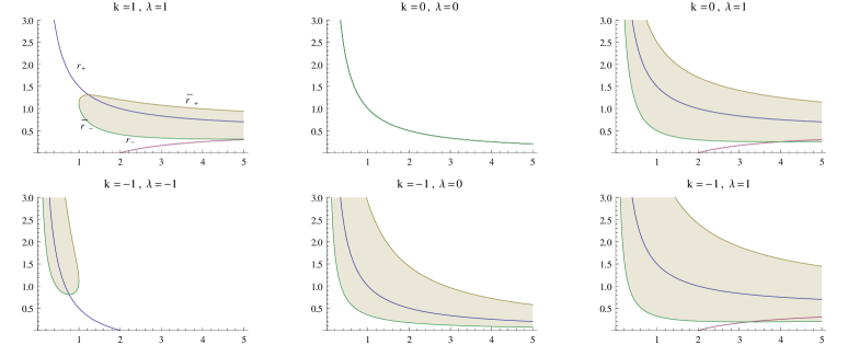
Figure 1: Plots of the horizon curves $\left(\frac{r_{\pm}}{R}\right)^{2}$ and $\left(\frac{\bar{r}_{\pm}}{R}\right)^{2}$ versus $a_{0}^{2}(t)$ for $C=\Lambda=2$ and various values for $k$ and $\lambda$. The shaded regions correspond to the regions where the diffeomorphism constructed above becomes singular, and hence the $(a,\tau)$ coordinate system breaks down. For $k=\lambda=0$ the horizons $r_{+}$ and $\bar{r}_{\pm}$ coincide, while for $k=\lambda=1$ and $k=\lambda=-1$ the regions $a_{0}<1$ and $a_{0}>1$ respectively must be excised since they are non physical – the solution ceases to be real. Due to the dilaton singularity at ${\bar{r}}_{+}$, the Wilson loop confines in the cosmological Liu-Tseytlin model [1] in all cases except for $k=\lambda=0$ and $k=\lambda=1$. For $k=\lambda=0$, the dilaton singularity is also present, the string tension however vanishes since ${\bar{r}_{+}}=r_{+}$, and $n(t,r_{+})=0$ as given in (8) vanishes in this case. For $k=\lambda=1$ there is a range of values $1\leq a_{0}\leq a_{0,\ast}$ for which $r_{+}>{\bar{r}}_{+}$, in which the Wilson loop touches the $r_{+}$ horizon for large quark separation and therefore shows perimeter law behavior. The transition point is given by $a_{0,\ast}$ as in (24). For later times $a_{0}>a_{0\ast}$, the Wilson loop will touch the ${\bar{r}}_{+}$ horizon and shows area law behavior. In this case we hence find a Wilson loop confinement-deconfinement transition. For a cosmological slicing of AdS-Schwarzschild [3] (i.e. constant dilaton backgrounds) the horizon structure is the same as for the cosmological Liu-Tseytlin model [1], in which case the Wilson loop show perimeter law behavor in all six cases. The situation is summarised in table 1.

2 Wilson Loops and the Quark-Antiquark Potential

The main result of [1] is the calculation of the static quark-antiquark potential from a fundamental string hanging from the boundary into the bulk space-time given by (6), at any fixed time $t$ and as a function of proper distance $L$, measured in the FRW metric (1). Following the standard procedure of calculating the embedding of a Nambu-Goto string, we found its tension

$$\tau_{q\bar{q}}(t)=\frac{n_{s}(r^{*},t)}{2\pi\alpha^{\prime}}=\frac{e^{\Phi(r,t)\over 2}}{2\pi\alpha^{\prime}}\left|\frac{a(r,t)n(r,t)}{a_{0}}\right|_{r^{\ast}}\,.$$ (23)

The quark-antiquark potential scales with the distance $L$ if $n_{s}(r,t)$ has a finite minimum at some distance $r=r^{*}$ outside the horizon ${\bar{r}}_{+}$ at a given $t$. We now evaluate the Wilson loop tension from the general result (23) for the dilaton solution given in (19), making use of additional information on the presence of an event horizon with diverging dilaton [5]. By plotting (23) numerically, we find that whenever ${\bar{r}_{+}}$ is the outermost horizon (i.e. the horizon with largest value of $r$) for a given “time” $a_{0}$ (all cases except $k=\lambda=0$ and $k=\lambda=+1$ in fig. 1), $n_{s}(r)$ diverges to $+\infty$ due to the dilaton divergence at the horizon, and hence the Wilson loop confines. In the absence of the ${\bar{r}}_{+}$ event horizon the Wilson loop can deconfine whenever the naive horizon at $r_{+}$ can be reached, as $n(r_{+},t)=0$, being the case for $k=\lambda=\pm 1$ in fig. 1 for a interval $1\leq a_{0}\leq a_{0,\ast}$. If neither $r_{+}$ or ${\bar{r}}_{+}$ horizons are present, as for e.g. $k=\lambda=-1$, at large $a_{0}$ the Wilson loop would confine again as the tension is finite at $r=0$, where space ends in these coordinates. The cases $\lambda=k=0$ and $\lambda=k=+1$ are special: In the former case the dilaton diverges at $r_{+}={\bar{r}}_{+}$, but the Wilson loop deconfines as this divergence is cancelled in (23) as $n(r,t)$ (c.f. eq. (8)) approaches zero at the same location. The latter case, $\lambda=k=+1$, shows a Wilson loop confinement-deconfinement transition: During the time interval $1\leq a_{0}\leq a_{0,\ast}$,

$$a_{0,\ast}^{2}=1-\sqrt{\frac{4C}{R^{2}}}+\sqrt{1+\frac{4C}{R^{2}}}\,,$$ (24)

the Wilson loop will reach the naive horizon (i.e. the horizon given by $n(r_{+},t)=0$), $r_{+}\geq{\bar{r}}_{+}$, and exhibit perimeter law behaviour. For $a_{0}>a_{0,\ast}$ on the other hand the Wilson loop will reach the event horizon ${\bar{r}}_{+}>r_{+}$ and exhibit area law behaviour, due to the dilaton singularity. We summarize the situation in table 1. We also note that the case $k=\lambda=-1$ does not allow for deconfinement transitions, despite the presence of the $r_{+}$ horizon, since cosmological evolution requires $a_{0}^{2}\leq 1$ such that the Wilson loop will not reach the naive $r_{+}$ horizon. In conclusion, except for the cases $k=\lambda=0$ and $k=\lambda=+1$, the Wilson loop is always confined during the cosmological evolution in the model of [1]. For $k=\lambda=0$ the Wilson loop is always deconfined, and for $k=\lambda=+1$ we find a transition from a deconfined state at early times to a confined state at later times.

	$\lambda=-1$	$\lambda=0$	$\lambda=+1$
$k=-1$	C , D	C , D	C , D
$k=0$		D , D	C , D
$k=+1$			D: $1\leq a_{0}\leq a_{0,\ast}$, C: $a_{0}>a_{0,\ast}$ , D

Table 1: (De)confinement (D/C) properties for cosmological Liu-Tseytlin [1] and AdS/Schwarzschild (i.e. constant dilaton) backgrounds [3]. The stated properties hold for all values of $a_{0}$ attained during cosmological evolution unless stated otherwise. The value of $a_{0,\ast}$ is given in (24).

3 Discussion

We revisited and extended the holographic backgrounds of [1] dual to $\mathcal{N}=4$ SYM on an FRW type cosmology and in the presence of a gluon condensate and instanton density, following the supersymmetric Ansatz of [5]. We found the most general solution of form (6) and introduced a (arbitrarily time-dependent) boundary cosmological constant $\lambda(t)$, which is equivalent to choosing an integration function in the bulk, the scale factor $a_{0}(t)$. We showed that the holographic stress-energy tensor is conserved for any $\lambda(t)$, clarifying conflicting claims between [1] and e.g. [10]. Furthermore, we found that these backgrounds are diffeomorphic to static black holes, whose event horizons become time-dependent in the cosmological frame, corresponding to a time-dependent observer viewing the static black hole event horizon. In the Liu-Tseytlin model [5] the dilaton diverges at the event horizon, covering the naive horizon $g_{tt}=0$ in most cases and in this way confining the Wilson loop. In two notable exceptions, $k=\lambda=0$ and $k=\lambda=+1$, the Wilson loop can reach the naive horizon $g_{tt}=0$ and deconfine. For $k=\lambda=+1$ this gives rise to a confinement-deconfinement transition. On the other hand, in the absence of the gluon condensate, i.e. in a cosmological slicing of AdS/Schwarzschild with a constant dilaton, the Wilson loop is expected to break on the event horizon and to deconfine. Both cases are summarized in table 1.

We conclude with several possibilities for future research: First, it would be interesting to construct other models with Wilson loop (de)confinement transitions (ideally at $k=0$, $\lambda>0$), and to apply the construction used here to other cases such as [12]. In such a model the free energy, another measure of (de)confinement, may also be calculated from holographic renormalization and linked to the Wilson loop behaviour. Finally, a further issue is the possible resolution of the dilaton singularity of [5].

References

• [1] J. Erdmenger, K. Ghoroku and R. Meyer, Phys. Rev.  D 84 (2011) 026004.
• [2] P. Binetruy, C. Deffayet, U. Ellwanger and D. Langlois, Phys. Lett.  B 477, 285 (2000).
• [3] P. S. Apostolopoulos et. al., Phys. Rev. Lett.  102 (2009) 151301; N. Tetradis, JHEP 1003 (2010) 040.
• [4] C. Charmousis, B. Gouteraux, B. S. Kim, E. Kiritsis and R. Meyer, JHEP 1011 (2010) 151.
• [5] H. Liu and A. A. Tseytlin, Nucl. Phys.  B 553 (1999) 231.
• [6] G. W. Gibbons, M. B. Green and M. J. Perry, Phys. Lett.  B 370, 37 (1996).
• [7] A. Kehagias and E. Kiritsis, JHEP 9911 (1999) 022.
• [8] A. Kehagias and K. Sfetsos, Phys. Lett.  B 456, 22 (1999).
• [9] D. Langlois, Phys. Rev.  D 62, 126012 (2000); D. Langlois and L. Sorbo, Phys. Rev.  D 68, 084006 (2003).
• [10] I. Papadimitriou, JHEP 1108 (2011) 119.
• [11] I. Papadimitriou and K. Skenderis, JHEP 0508 (2005) 004.
• [12] T. Sakai and S. Sugimoto, Prog. Theor. Phys.  113 (2005) 843; Prog. Theor. Phys.  114 (2005) 1083.