A near-infrared study of the star forming region RCW 34

Abstract

We report the results of a near-infrared imaging study of a $7.8\times 7.8$ arcmin² region centered on the 6.7 GHz methanol maser associated with the RCW 34 star forming region using the 1.4m IRSF telescope at Sutherland. A total of 1283 objects were detected simultaneously in J, H, and K for an exposure time of 10800 seconds. The J-H, H-K two-colour diagram revealed a strong concentration of more than 700 objects with colours similar to what is expected of reddened classical T Tauri stars. The distribution of the objects on the K vs J-K colour-magnitude diagram is also suggestive that a significant fraction of the 1283 objects is lower mass pre-main sequence stars. We also present the luminosity function for the subset of about 700 pre-main sequence stars and show that it suggests ongoing star formation activity for about $10^{7}$ years. An examination of the spatial distribution of the pre-main sequence stars shows that the fainter (older) part of the population is more dispersed over the observed region and the brighter (younger) subset is more concentrated around the position of the O8.5V star. This suggests that the physical effects of the O8.5V star and the two early B-type stars on the remainder of the cloud out of which they formed, could have played a role in the onset of the more recent episode of star formation in RCW 34.

1 Introduction

Studies on star formation can very broadly be classified as either the study of the process of star formation as such or as the study of the larger scale processes that trigger star formation in molecular clouds and which determines the mode of star formation, ie. clustered or distributed star formation. Although large strides have been made over the last couple of decades in understanding the process of star formation, an understanding of what determines the mode of star formation, which is equally important to understanding the process of the formation of individual stars, is still lacking. The two aspects are, obviously, not independent of each other and together play a role in determining important properties such as, for example, the stellar initial mass function and the star formation efficiency. To achieve the goal of a theoretical understanding of the physical process determining the mode of star formation, empirical information on a sufficiently large sample of embedded young clusters is necessary (Lada, 2010). The present near-infrared study of RCW 34 attemps to add to this effort.

RCW 34 is a southern high mass star forming region that has been studied at irregular intervals over a number of decades. The number of observational studies that was directly aimed at investigating RCW 34 is quite small. We review those that are relevant to the present study. RCW 34 was first catalogued by Rodgers et al. (1960) as one of the southern $\mathrm{H\alpha}$ emission regions with a diameter less than 2 $\times$ 2 arcminutes. The exciting star of RCW 34 also appears in the catalogue of stars in reflection nebulae compiled by van den Bergh & Herbst (1975). Based on this catalogue the exciting star in RCW 34 is also refered to in the literature as either Vela R2 25a or vdBH 25a. Following up on the catalogue of van den Bergh & Herbst (1975), Herbst (1975a) did UBV and MK spectroscopy on the stars in the catalogue and classified the exciting star in RCW 34 as of spectral type O9. In a further analysis of the UBV data, Herbst (1975b) did main-sequence fitting on the stars of Vela R2 association. This resulted in a distance of about 870 pc to the association. However, the exciting star of RCW 34 was found to lie well below the ZAMS, which lead Herbst (1975b) to consider it to be peculiar. Herbst (1975b) explained the position of RCW 34 well below the ZAMS as due to it being either an O star located further than the Vela R2 association or an O-type pre-main sequence star with a “grey” circumstellar shell associated with Vela R2. Vittone et al. (1987) was the first to follow up on the finding of Herbst (1975b) that the exciting star of RCW 34 lie well below the ZAMS for the Vela R2 association. These authors also concluded that vdBH 25a is an O9 type star but that the distance to the star is uncertain.

The first really comprehensive study of RCW 34 aimed to answer the questions on the nature of vdBH 25a and its distance is that of Heydari-Malayeri (1988). Using a variety of observations and data from the literature, Heydari-Malayeri (1988) concluded that RCW 34 is located at 2.9 kpc, well beyond the Vela R2 association, and that its exciting star is a heavily reddened (A_v = 4.2) O8.5V ZAMS star. There is therefore nothing peculiar about the exciting star of RCW 34. Heydari-Malayeri (1988) also interestingly remarks that the presence of an $\mathrm{H_{2}O}$ maser might signify ongoing star formation in RCW 34.

The most recent study of RCW 34 is that of Bik et al. (2010). These authors made near-infrared H- and K-band observations on a $104^{\prime\prime}\times 60^{\prime\prime}$ field centered on the O8.5V ionizing star, using the Integral Field instrument SINFONI on UT4 of the VLT at Paranal, Chile. In addition they also used archival data obtained with IRAC (Fazio et al., 2004) on board the Spitzer satellite. Using this data Bik et al. (2010) identified three regions associated with RCW 34: The first is a large bubble detected in the IRAC images in which a cluster of intermediate- and low-mass class II objects is found. The second is the H II region located at the northern edge of the bubble and which is ionized by three OB stars. The third region is a photon-dominated region north of the H II region and which marks the edge of a dense molecular cloud traced by H₂ emission. Several class 0/I objects associated with this cloud were also identified indicating recent star formation activity. Bik et al. (2010) revised the distance to RCW 34 to 2.5 $\pm$ 0.2 kpc and derived an age estimate of 2 $\pm$ 1 Myr from the properties of the pre-main sequence stars inside the H II region.

The observations presented here differ from earlier near-infrared (NIR) observations, and in particular from that of Bik et al. (2010) in that we imaged a 7.8^′ $\times$ 7.8^′ region centered on the 6.7 GHz methanol maser located at coordinates $\mathrm{\alpha(2000)=08^{h}56^{m}24^{s}.9}$ and
$\mathrm{\delta(2000)=-43^{\circ}05^{\prime}40^{\prime\prime}.4}$. This is significantly larger than the 104^′′ $\times$ 60^′′ region covered by Bik et al. (2010). This much larger field gives us the opportunity to also investigate possible star formation activity especially to the north of the shocked region where the H II region interacts with the molecular cloud and created a photo-dissociation region (Bik et al., 2010). Except for the class II methanol maser which indicates the presence of a very young high mass star there appears to be no other signs of current high mass star formation activity to the north of the H II region. This does not exclude the presence of lower mass stars, however.

Within the framework of a broader view on star formation as outlined above, our results should be seen as complimentary to that of eg. Bik et al. (2010) and others which can help to understand the star formation history of RCW 34. Our aim here is to present some basic properties of the embedded cluster associated with RCW 34 as derived from our NIR observations.

2 Observations, data reduction, and calibration

The observations used in this study can be regarded as archival data in the sense that the data were not collected by the authors themselves for the primary purpose of studying RCW 34 as is done here. The data used here was collected by GG Nyambuya in 2005, however, for a completely different purpose. This caused the data to be lacking in certain aspects, for example in that there were no control field observations.

The observations were made on the nights of 2005, April 18, 22 and 25 with the SIRIUS (Simultaneous-three-colour Infrared Imager for Unbiased Survey) camera of the Infra Red Survey Facility’s 1.4m telescope located at the SAAO’s Sutherland observatory. SIRIUS has three science-grade HAWAII 1024 $\times$ 1024 arrays with two dicroic mirrors which enable simultaneous observations in $J$ ($\lambda=1.25\mu m)$, $H$ ($\lambda=1.65\mu m)$ and $K_{s}$ ($\lambda=2.25\mu m)$. Precise colour information can thus be obtained with such simultaneous observations. The atmospheric conditions for the three nights gave a FWHM for the seeing disk of 1.1 to 1.4 arcsec for images in the $K_{s}$ band. The field of view was 7.8 $\times$ 7.8 arcmin² with a pixel scale of 0.45 arcsec per pixel.

The total exposure of the observations consisted of three nights of 12 dithered sets per night, each set consisting of 10 ditherings of 30s each. This resulted in a total exposure time of 10800 seconds for the three nights. The initial data reduction was done at the University of Cape Town using the SIRIUS pipe-line software which include all the basic reduction steps such as dark subtraction, flat fielding, and sky subtraction to produce a single image for one night’s observations. The images of the three nights were median combined to produce a final image.

The IRAF task DAOFIND was used to select stars from the field. In total 1283 objects were detected in all three bands. The instrumental magnitudes were calibrated to the 2MASS system. This was done by selecting 40 stars in the observed field detected in J, H, and K for both the IRSF and 2MASS and for which the world coordinates of both sets agreed such that the cross identification between the IRSF and 2MASS is unique. The correlation between IRSF instrumental and 2MASS apparent magnitudes as well as between IRSF colours and 2MASS colours of the 40 stars were investigated. This led to the following equations transforming IRSF instrumental magnitudes to 2MASS apparent magnitudes:

$$\mathrm{J_{2mass}} = \mathrm{J_{IRSF}+0.1175(J-H)_{IRSF}}-4.2318$$

$$\mathrm{H_{2mass}} = \mathrm{H_{IRSF}-0.0761(H-Ks)_{IRSF}}-4.0974$$

$$\mathrm{Ks_{2mass}} = \mathrm{Ks_{IRSF}+0.0240(H-Ks)_{IRSF}}-5.0834$$

Following this calibration our observations reached J = 19.79, H = 18.43, and K_s = 17.64.

It is also necessary to comment on adopting a distance of 2.5 kpc to RCW 34 before presenting the results. It has already been noted that Heydari-Malayeri (1988) asigned a distance of 2.9 kpc to RCW 34 also using the spectral type of the exciting star. Bik et al. (2010) pointed out that the difference between their distance estimate and that of Heydari-Malayeri (1988) lies in the different absolute magnitudes used. Two kinematic distance estimates for RCW 34 are also available. The water maser associated with RCW 34 has a velocity $\mathrm{V_{lsr}=10.8~{}km\,s^{-1}}$ (Braz & Scalise, 1982). Using the rotation curve of Wouterloot & Brand (1989) this gives a distance of 2.1 kpc. The second kinematic distance comes from the velocity of the radio recombination line associated with the H II region. Caswell & Haynes (1987) gives this as $\mathrm{12~{}km\,s^{-1}}$ which translates to a distance of 2.3 kpc, again using the rotation curve of Wouterloot & Brand (1989). Although a detailed analysis of the uncertainties of each of the four estimates can be made to decide which to use, it seems more appropriate for the present to use the mean of the four estimates which is 2.45 kpc. It therefore seems reasonable to simply use the distance estimate of Bik et al. (2010), ie. 2.5 kpc.

3 Results and analysis

3.1 The two-colour diagram

The NIR J-H, H-K two colour diagram has been used in the past by numerous authors to present NIR photometry of young stellar populations and to identify different types of objects. Here we follow the same practice. The main result of the present study is presented in Fig. 1. The main sequence and giant branch were taken from Koornneef (1983) and transformed to the 2MASS system. Four reddening lines using the extinction law of Rieke & Lebofsky (1985) are also shown. $\mathrm{R_{1}}$ and $\mathrm{R_{2}}$ are the reddening lines that bracket the main sequence and giant branch while $\mathrm{R_{3}}$ is the reddening line for a star of spectral type F0, which is more or less the upper mass limit for T Tauri stars. Weak line T Tauri stars (WTTS) have intrinsic NIR colours consistent with those of normal dwarf stars (Lada & Adams, 1992; Meyer et al., 1997) and should therefore fall between reddening lines R₁ and R₃. The solid green line gives the classical T Tauri star (CTTS) locus from Meyer et al. (1997) and the dashed green lines the upper and lower boundaries as calculated from the errors given by these authors. The meaning of reddening line R₄ is quite obvious.

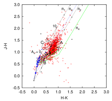
Figure 1: Near-infrared two-colour diagram for 1283 objects (red crosses) detected in J, H, and K. Blue triangles are WTTS from Strom et al. (1989) and black dots CTTS from Strom et al. (1989) and Cieza et al. (2005).

We broadly identify three groupings or clusterings of objects on the two-colour diagram, with the area that each more or less cover indicated by the ellipses in Fig. 1. Group A is a strong clustering of objects extending along and on both sides of reddening line R₂ just above its intersection with the CTTS locus and is the most obvious aspect of the distribution of the 1283 objects on the two-colour diagram. Above reddening line R₂ most of the group A objects lie between reddening lines R₂ and R₃. There also seems to be a band of objects starting from the A_V = 10 point on reddening line R₂ and extending almost along the CTTS locus to the lower left with most of the objects lying inside the boundaries of the CTTS region although some lie just above the upper boundary. This is group B. Group C is a very loose group of objects that lie to the left of group A. The reason for identifying group C is mainly because there seems to be a gap between the bluer objects in group B and the objects in group C.

It is also seen that there are highly reddended objects with visual extinctions around 20 as well as objects with very large infrared excesses. For the present we focus mainly on trying to understand group A which is the most obvious feature of the distribution on the two colour diagram.

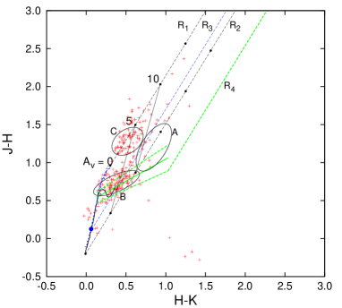
Figure 2: Near-infrared two-colour diagram for IRSF objects brighter than J = 16.21 magnitude.

Given the distribution of objects on the two-colour diagram in Fig. 1 the question might be asked as to the reality of the clustering and the nature of the objects belonging to group A. Although in NIR studies of other star forming regions it is not uncommon to find objects in the same region on the two-colour diagram as that of group A, the large number of objects in the case of RCW 34, is uncommon. The fact that the SIRIUS camera has three independent arrays means that the detection of an object in all three the NIR bands implies a real detection and not some artifact on the array. The existence of a large number of objects with NIR colours as reflected by the group A objects should therefore be regarded as real. Since we have no spectroscopic identification of any of the objects it is necessary to proceed without such information.

Focusing attention on the group A objects, we note the following. First, they cluster just above the CTTS locus. In fact it would seem as if the CTTS locus acts as an approximate lower boundary for these objects on the two-colour diagram. Second, a significant fraction of the objects lie to the right of reddening line R₂. These objects have an infrared excess and cannot be dereddended to the main sequence. It is also seen that a further significant fraction of the remainder of the group A objects lie above the CTTS locus and between reddening lines R₂ and R₃. Although these objects can be dereddened to the main sequence, such a dereddening would imply the presence of a very large number of stars of spectral type earlier than F0. Although the visual extinction of these stars would be between 10 and 15 magnitudes, the dereddening would also result in some being ionizing stars which definitely would have been detected as H II regions in radio continuum surveys or as bright infrared sources. Only three OB stars are, however, associated with RCW 34 (Bik et al., 2010).

We note that in some studies similar to the present one, such as eg. that of Dahm & Simon (2005) and Barentsen et al. (2011), use has been made of 2MASS for the NIR photometry. Inspection of the magnitudes of the 2MASS objects in the same field covered by the present IRSF observations showed that the limiting J-band magnitude is 16.12 for objects detected simultaneously in J, H, and K. Figure 2 shows the two-colour diagram for IRSF detections with J magnitude brighter than 16.12. What is important to note is the near absence of objects in the group A region. On the other hand, it is seen that there still are quite a number of objects in group B. This suggests that the majority of the group A objects is a population of fainter objects revealed by our significantly deeper imaging of RCW 34 compared to 2MASS. As already argued, it seems unlikely that the group A objects are simply reddened main-sequence stars. To avoid a completely skewed IMF they rather seem to be lower mass objects associated with the RCW 34 star forming region.

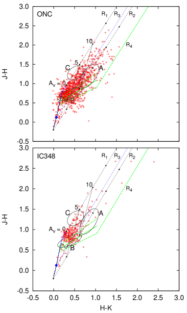
Figure 3: Near-infrared two-colour diagrams for the Orion Nebula Cluster (top panel) and IC 348 (lower panel).

The fact that the group A objects cluster above the CTTS locus is suggestive that they might be reddended CTTS. Some early NIR imaging of embedded clusters such as eg. IC348 (Lada & Lada, 1995), NGC1333 (Lada et al., 1996), L1630 (Li et al., 1997), as well as some more recent imaging eg. in the cases of NGC 2316 (Teixeira et al., 2004) and the Horsehead Nebula (Bowler et al., 2009) do not show similar large numbers or even has a lack of apparent CTTS’s. This may well be due to these surveys not being deep enough or that intrinsically there is an absence of large numbers of CTTS in these star forming regions. Although not in such large numbers as in the case of RCW 34, other star forming regions such as eg. NGC 7538 (Balog et al., 2004) do show a significant number of cluster members which, in terms of Fig. 1, lie just below reddening line R₂ and thus can not be dereddened to the main-sequence as is also the case for RCW 34. Similarly, for AFGL5180 (Devine et al., 2008) quite a significant fraction of the objects on the two-colour diagram lie below the reddening line R₂ but above the T Tauri locus of Meyer et al. (1997).

In all of the above mentioned studies objects lying to the right of reddening line R₂ and above the T Tauri locus are regarded as pre-main sequence stars. In fact, Lada & Adams (1992) have shown that pre-main sequence stars classified as CTTS based on the equivalent widths of their H$\alpha$ emission lie in the group A region. Other studies eg. that of Strom et al. (1989), Cieza et al. (2005), Luhman et al. (1998), and Barentsen et al. (2011) confirm this. In Fig. 1 we also show the positions of the spectroscopically identified CTTS from Strom et al. (1989) and Cieza et al. (2005) as well as the WTTS from Strom et al. (1989). It is seen that the spectroscopically identified CTTS are associated with the group A and B regions. Luhman et al. (1998) also found that for IC 348 sources showing signs of disk activity are associated with our group A objects.

As examples and for comparison with RCW 34 we show in Fig. 3 the two-colour diagrams for the Orion Nebula Cluster (ONC), using the data of Hillenbrand et al. (1998), and IC 348, using the data of Luhman et al. (2003). It is seen that while the ONC has quite a number of objects in region A (which we will later use), on the other hand IC 348 has very few. None of the two, however, has the same clustering as seen in RCW 34.

Considering the above, a preliminary conclusion is that the group A objects are most likely lower mass pre-main sequence stars and that some of the group B objects, although not having an infrared excess, might also be T Tauri stars.

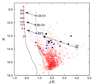
Figure 4: Colour-magnitude diagram for RCW 34. The red crosses are the objects detected with the IRSF. The solid black line is the unreddened main sequence for a distance of 2.5 kpc. The dashed line is the corresponding main-sequence reddened with A_V = 5.1 magnitudes. Blue triangles and solid squares are respectively the late-type main sequence stars and pre-main sequence stars from Bik et al. (2010).

3.2 The colour-magnitude diagram.

In Fig. 4 we show the K vs J-K colour-magnitude diagram (CMD) for the 1283 objects detected in J, H, and K with the IRSF (red crosses). We use the JK CMD in order to compare the positions of the spectroscopically identified late-type and pre-main sequence stars of Bik et al. (2010) (taken from their Table 6) with our NIR detections. The main-sequence (solid line) was taken from the Padova models (Marigo et al., 2008) and has been adjusted for distance only using a distance of 2.5 kpc to RCW 34. The red dots on the main sequence are the positions of the more massive main sequence stars with their masses (in solar masses) given to the left of each point. We also show in Fig. 4 the positions of those stars for which Bik et al. (2010) were able to determine spectral types from the SINFONI observations. The blue triangles are the main sequence stars and the solid black squares the late-type pre-main sequence stars. Although there is some overlap in the J-K colours of the two groups, it is seen that, except for one case, the pre-main sequence stars are on average redder than the main-sequence stars. The reddest object in the list of Bik et al. (2010) is star 24, with J-K $\sim$ 4. It is classified as an early K-type dwarf by Bik et al. (2010) but of uncertain luminosity class. Its position is also shown in Fig. 4.

It is seen that the objects detected with the IRSF populate a very specific area on the CMD. Most of the objects have $\mathrm{K<14}$ and $1<\mathrm{J-K}<3$ with a clustering around K $\lesssim$ 16 and J-K $\sim$ 2. The effect of the limited sensitivity of our imaging is also clearly visible as the sharp cutoff on the lower right hand side of the region covered by the IRSF objects. Inspection of the equivalent CMD of Bik et al. (2010) (their Figure 7) shows that these authors also detected some objects that lie between K magnitudes 14 and 16 and for J-K just less than 2 there is a clustering of objects to the right of the main sequence. Our imaging also shows a large number of objects at that position on the colour-magnitude diagram.

Using the visual extinctions calculated by Bik et al. (2010) (their Table 4) we also calculated the dereddened positions of the three early-type stars as well as that of star 24. The dereddening vectors are shown by the arrows starting at each of the stars. For the three early-type stars the dereddended positions do not fall exactly on the main sequence but slightly to the right. Adding a further approximately 0.9 visual magnitudes will bring the three dereddened early-type stars on the main sequence. However, we noted that there is a difference in extinction for the three OB stars as given in Tables 4 and 6 of Bik et al. (2010). For example for star 1, the exciting star, Table 4 gives an extinction of 4.2 while it is given as 4.8 in Table 6. The reason for this not clear. We also note that the extinction toward region II of Bik et al. (2010) (see their Figure 4), which is close to the location of the three OB stars, is A_v = 5.1 magnitudes. The required visual extinction of 5.1 magnitudes to bring the unreddened main sequence to the positions of the three OB stars is therefore in general agreement with the measurements of Bik et al. (2010). It is furthermore interesting to note that star 24, with an estimated extinction of $15.9\pm 2.8$ cannot be dereddened at all to the main sequence and if it could, it would not be a K-dwarf. Star 24 is therefore most likely still in the pre-main sequence phase.

Taking the three OB stars’ positions to indicate the position of the reddened main sequnce, we can redden the unreddened main sequence accordingly. This is shown as the dashed line in Fig. 4. It is seen that the majority of our IRSF sources still lie significantly to the right of the main sequence as will be expected for pre-main sequence stars. This result is in support of our hypothesis that the sample of 1283 objects detected in J, H, and K contains a significant number of pre-main sequence stars. Those objects lying significantly to the left of the reddened main sequence are most probably foreground stars.

3.3 The luminosity function

The luminosity function is an important characteristic of the population of pre-main sequence stars since it contains information about the age, initial mass function, and star formation history of that particular population. In constructing the luminosity function and estimating the ages of members of the population the ideal would be to know the effective temperature and luminosity of each individual star from spectroscopic measurements and to then construct a luminosity-temperature diagram on which model isochrones can overlaid to estimate the pre-main sequence ages. In the present case we only have NIR photometry data which is not suitable to determine stellar effective temperatures due to contamination from excess emission from circumstellar material. Uncertainties in the photometry can also lead to erroneous conclusions about the ages of individual objects (see eg Preibisch (2012) for an extensive discussion).

However, as argued by Bontemps et al. (2001), the $J$-band flux is least affected by contamination from circumstellar emission and is close to the peak of the photospheric spectral energy distribution for these cool stars and may be used to estimate stellar luminosities. We therefore followed these authors and estimated the stellar luminosity directly from the absolute $J$-band magnitude using the relation (Bontemps et al., 2001)

$$\log_{10}(L_{\star})=1.49-0.466\,M_{J}$$ (1)

The estimated uncertainty on $\log_{10}(L_{\star})$ using Eq. 1 is 0.19 dex.

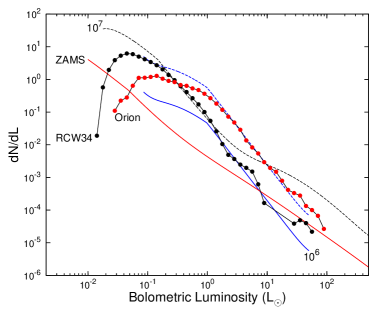
Figure 5: Bolometric luminosity distribution for a subset 745 infra-red excess sources(black dots). The blue, dashed black, and red lines are the single stellar population luminosity functions respectively at $10^{6}$ and $10^{7}$ years and for the ZAMS as calculated from the mass-luminosity relations at these times as given by the models of Siess et al. (2000). The luminosity function for Orion is given by the black line with red dots.

Application of Eq. 1 requires calculation of the absolute $J$-band magnitude and therefore dereddening of the observed $J$-band magnitudes. The assumption was therefore made that all the group A objects are reddened CTTS. However, we selected only the subset of 745 group A objects that lie to the right of reddening line R₃, above the T-Tauri locus and with $0.53<\mathrm{H-K}<1$. These objects all have an infrared excess and cannot be dereddened to the main sequence. Since we do not know the true unreddened intrinsic colours, each object was dereddened to a random position between the upper and lower boundaries of the T Tauri locus but still lying on its individual dereddening line. One instance of dereddening all 745 objects then results in a luminosity function for the given random positions around the T Tauri locus. By repeating the procedure a large number of times it is possible to construct an average luminosity function that is representative of a large number of realizations of intrinsic colours for the dereddened objects. All objects were assumed to lie at a distance of 2.5 kpc to calculate the absolute magnitudes and therefore the stellar luminosities.

In Fig. 5 we show with the black solid line the luminosity function averaged over 1000 dereddening realizations and normalized such that $\int(dN/dL)dL=1$. Normalization is necessary to be able to compare the luminosity functions of different star forming regions as we will do below. The distribution is seen to have a peak at about 0.04$\mathrm{L_{\odot}}$ below which there is a sharp cut-off which most likely is a sensitivity effect. Except for the last three highest luminosities, the luminosity function follows a power law with an index of $-2.34\pm 0.07$ for luminosities above about 0.3 $\mathrm{L_{\odot}}$.

The observed luminosity distribution is a result of the combination of the evolution of the pre-main sequence mass-luminosity relation with time, the underlying initial mass function and the star formation history of the region. We attempted to interpret the observed luminosity distribution with single stellar population (SSP) luminosity functions constructed by using the mass-luminosity relation for pre-main sequence isochrones at $10^{6}$ and $10^{7}$ years and the ZAMS from the Siess et al. (2000) models combined with a Kroupa stellar initial mass function (Kroupa, 2001) for masses between 0.3 $\mathrm{M_{\odot}}$ and 2 $\mathrm{M_{\odot}}$. For an SSP the luminosity function, $dN/dL$, is related to the initial mass function, $dN/dm$, as $dN/dL=(dN/dm)\times(dm/dL)$. To calculate $dm/dL$ we approximated the mass-luminosity relation, as given by the Siess et al. (2000) model for a specific isochrone, on a log-log scale with a polinomial which is easily differentiable. The use of the $10^{6}$ and $10^{7}$ year luminosity functions as comparison with the observed luminosity function should not be interpreted as attemps for absolute age estimates but as guides to interpret the observed luminosity function. The result of this calculation is shown in Fig. 5 where the luminosity functions at $10^{6}$ (blue solid line) and $10^{7}$ (dashed black line) years have been adjusted vertically to more or less coincide with parts of the observed luminosity function of RCW 34. The luminosity function for the ZAMS (solid red line) has been placed at an arbitrary position.

Inspection of Fig. 5 shows that although the observed luminosity function can be fitted by a single power law for $\mathrm{L>0.3\,L_{\odot}}$, neither of the $10^{6}$ or $10^{7}$ year SSP luminosity functions can explain the entire observed luminosity function. It is seen that the theoretical $10^{6}$ year luminosity function explains the observed luminosity function rather well for luminosities greater than about $\mathrm{1.4\,L_{\odot}}$. Below $\mathrm{\sim 1.4\,L_{\odot}}$ the theoretical luminosity dips below the observed luminosity function, suggesting the presence of an older component. The theoretical luminosity function for an SSP with an age of $10^{7}$ years is seen to follow the observed luminosity function quite well between $\mathrm{\sim 0.2\,L_{\odot}}$ and just less than $\mathrm{1.4\,L_{\odot}}$. For $\mathrm{L\lesssim 0.2\,L_{\odot}}$ the observed luminosity function starts to bend away from and fall below the theoretical $10^{7}$ year luminosity function. This behaviour is most certainly due to the limited sensitivity of our imaging. Finally we note that the observed luminosity function nowhere has the behaviour of the luminosity function for the ZAMS suggesting that the group A objects used here are not main sequence objects.

The fact that a significant part of the RCW 34 luminosity function can be explained by a combination of the $10^{6}$ and $10^{7}$ year SSP luminosity functions is suggestive that star formation in RCW 34 has been an ongoing process for about $10^{7}$ years. As already noted, based on the presence of the O8.5V star that powers the H II region, Bik et al. (2010) put an upper limit of $8\times 10^{6}\sim 10^{7}$ years on the age of RCW 34. The presence of a class II methanol maser indicates a much more recent episode of star formation activity associated with RCW 34 since these masers are known to be exclusively associated with a very early phase of massive star formation (Ellingsen, 2006). Furthermore, the 6.7 GHz methanol maser lifetime is estimated to be between $2.5\times 10^{4}$ and $4.0\times 10^{4}$ years (van der Walt, 2005). From their set of 26 spectroscopically identified pre-main sequence stars Bik et al. (2010) estimate the age of the youngest pre-main sequence objects to be $(2\pm 1)\times 10^{6}$ years. Our analysis of the NIR photometric data of a completely different sample of objects in RCW 34 is therefore in general agreement with that of Bik et al. (2010).

In Fig. 5 we also show the luminosity function for 204 pre-main sequence stars from the Orion Nebular Cluster using the data of Hillenbrand et al. (1998). The JHK colours of all the objects in the catalog of Hillenbrand et al. (1998) were transformed from the CIT to the 2MASS system and afterwards subjected to the same selection criteria that was used to select the subset of 745 group A sources from which the RCW 34 luminosity function constructed. Dereddening was done in the same way as for the RCW 34 sources and an average luminosity function was calculated over 1000 dereddening realizations.

For the Orion sources the luminosity function peaks at about 0.1 $\mathrm{L_{\odot}}$ compared to 0.04 $\mathrm{L_{\odot}}$ for RCW 34. The Orion luminosity function crosses the RCW 34 luminosity function between 0.2 and 0.3 $\mathrm{L_{\odot}}$. For L $\gtrsim$ 2 $\mathrm{L_{\odot}}$ the two luminosity functions runs almost parallel to each other except for the last two points for RCW 34. In fact, the main trend of the ONC luminosity function for $\mathrm{L>2\,L_{\odot}}$ is a power law with index -2.17 $\pm$ 0.05 which is very similar to that of RCW 34. It is also seen that for $\mathrm{L\geq 2~{}L_{\odot}}$ the $10^{6}$ year SSP luminosity function (dashed blue line) describes the Orion luminosity function quite well. This is in agreement with independent age estimates of about $2\times 10^{6}$ years for the ONC (see eg. Reggiani et al., 2011). Comparison of the $10^{6}$ and $10^{7}$ year SSP luminosity functions suggest that the slope of the luminosity function for $\mathrm{L>2\,L_{\odot}}$ is definitely dependent on the age of the system. Thus, just by comparison of the luminosity function of RCW 34 with that of the ONC already suggests the existence of component with an age of about 1 - 2$\times 10^{6}$ years in RCW 34.

3.4 Spatial distribution of objects.

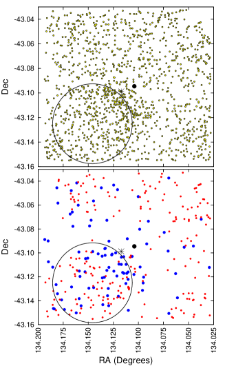
Figure 6: Top panel: The spatial distribution of all 1283 objects. Bottom panel: Spatial distribution for 91 objects with $\mathrm{L>0.5\,L_{\odot}}$ (blue dots) and 209 objects with $\mathrm{L<0.075\,L_{\odot}}$ (red dots). The black dot indicates the position of the 6.7 GHz methanol maser and the star the position of the O8.5V star. The circle in the top and bottom panels indicates the approximate size and location of the opacity hole (bubble) as revealed in the dust emission of the region (See eg. Figs. 1 & 3 of Bik et al., 2010). Note that the coordinates are in decimal degree.

In the top panel of Fig. 6 we show the spatial distribution of the 1283 objects detected in J, H and K. Some degree of clustering can be seen in a short band running north-east to south-west just south of the central O8.5V star. Otherwise, the detected objects seems to be more or less uniformly distributed over the field.

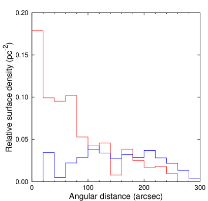
Figure 7: Radial surface density distribution of group A objects with luminosity greater than 0.5$\mathrm{L_{\odot}}$ (red line) and objects with luminosity less than 0.075$\mathrm{L_{\odot}}$ (black line). The origin was taken as the position of the O8.5V star.

Given that our analysis of the luminosity function suggests that star formation in RCW 34 took place over an extensive period of time, the question is whether there is any difference in the spacial distribution of the younger and older pre-main sequence stars. Here we follow the discussion in the previous section and use luminosity as an approximate indicator of age with younger objects having greater luminosity than older ones. To ensure that we have a statistically sufficient number of objects we select the brighter objects as those with $\mathrm{L>0.5\,L_{\odot}}$. This resulted in 91 objects. For the older group we selected the 209 objects with $\mathrm{L<0.075\,L_{\odot}}$. The spatial distribution of the two groups is shown in the bottom panel of Fig. 6

Inspection of the bottom panel of Fig. 6 suggests a clustering of the higher luminosity objects (younger ones; blue dots) closer to the O8.5V star than the fainter objects (red dots) and in particular in the region of the opacity hole. To quantify the distributions we calculated the relative surface density of younger and older objects as a function of distance from the O8.5V star using a number of annulli. The two distributions are shown in Fig. 7. The brighter objects clearly shows a significantly higher probability of being found closer to the O8.5V star than the fainter objects which have a flatter surface density distribution. In both cases the decrease in the surface density beyond $\sim$240 arcsec is artificial and due to the fact that we have not corrected the larger annulli for the smaller surface area enclosed inside the frame borders.

Reggiani et al. (2011) recently also investigated the variation of the surface density distribution of pre-main sequence stars with age in the ONC. Interestingly enough these authors found that the older objects have a less concentrated distribution compared to the younger objects. Qualitatively the same behaviour is seen in RCW 34. However, it should be kept in mind that the older lower mass stars are most probably of the same age as the three OB stars. The concentration of the younger group closer to the three OB stars seems to suggest that the more recent episode of star formation may have been triggered by the presence of these three stars.

4 Summary and Conclusions

We presented NIR imaging data on RCW 34 for a $7.8\times 7.8$ arcmin² region centered on the 6.7 GHz methanol maser associated with RCW 34. A total of 1283 objects were detected in J, H, and K-bands. The distribution of these objects on the two-colour diagram shows a concentration of more than 750 objects for which the colours are the same as that of confirmed classical T Tauri stars found in other star forming regions. Given that the position of the main sequence on the K vs J-K CMD is determined by the positions of the three OB stars, the distribution of the IRSF sources on the CMD is also suggestive that a significant number of these are lower mass pre-main sequence stars.

We also constructed the bolometric luminosity function for the 745 objects and showed that parts of the luminosity function can be explained by SSP luminosity functions with ages of $10^{6}$ and $10^{7}$ years. The presence of a young component in the stellar population of RCW 34 is in agreement with the results of Bik et al. (2010) based on 26 spectroscopically identified pre-main sequence stars as well as the presence of a class II methanol maser which indicate a very recent episode of massive star formation. Our estimate of $10^{7}$ years for the age of an older component is qualitatively in agreement with the main sequence life times of the three OB stars associated with RCW 34.

Whereas previous studies of RCW 34 focused more on the central region around the ionizing star, our NIR imaging revealed a more spread out population of low mass pre-main sequence stars. The younger stars appear to be more concentrated in the central region around the O8.5V star while the older pre-main sequence stars seems to be more spread out.

Considering our NIR results as well as that of Bik et al. (2010), RCW 34 seems to be a much more interesting star forming region than was perhaps previously thought. First, there appears to be a very large number of low mass stars formed over a period of about $10^{7}$ years with the older being more spread out than the younger component. Second, it seems rather certain that massive star formation in RCW 34 took place in two separate events with only three OB stars forming in the first event and most probably only a single massive star, as evidenced by the 6.7 GHz maser, forming in the most recent event. The fact that the brighter (younger) lower mass pre-main sequence stars seems to cluster around the position of the three OB stars strongly suggests that that the physical effects these three stars had on the remainder of the molecular cloud from which they formed could have played a role in the more recent episode of star formation. Obviously our photometric study need to be followed up by a spectroscopic study which we plan to do. Apart from verifying our photometric identifications, will such a study be very usefull to also try to unravel the star formation history, especially of the low mass stars, in RCW 34. Given that there also seems to be a significant number of low mass pre-main sequence stars spread out almost uniformly over the $7.8\times 7.8$ arcmin² region might require a different scenario for the star formation history in RCW 34 than that suggested by Bik et al. (2010). Although RCW 34 cannot be regarded as peculiar anymore, it is seems to be interesting and sufficiently different from other star forming regions to require further investigation.

References

- Balog et al. (2004) Balog, Z., Kenyon, S. J., Lada, E. A., Barsony, M., Vinkó, J., & Gáspaŕ, A. 2004, AJ, 128, 2942
- Barentsen et al. (2011) Barentsen, G., et al. 2011, MNRAS, 415, 103
- Bik et al. (2010) Bik, A., et al. 2010, ApJ, 713, 883
- Bontemps et al. (2001) Bontemps, S., et al. 2001, A&A, 372, 173
- Bowler et al. (2009) Bowler, B. P., Waller, W. H., Megeath, S. T., Patten, B. M., & Tamura, M. 2009, AJ, 137, 3685
- Braz & Scalise (1982) Braz, M. A., & Scalise, Jr., E. 1982, A&A, 107, 272
- Caswell & Haynes (1987) Caswell, J. L., & Haynes, R. F. 1987, A&A, 171, 261
- Cieza et al. (2005) Cieza, L. A., Kessler-Silacci, J. E., Jaffe, D. T., Harvey, P. M., & Evans, II, N. J. 2005, ApJ, 635, 422
- Dahm & Simon (2005) Dahm, S. E., & Simon, T. 2005, AJ, 129, 829
- Devine et al. (2008) Devine, K. E., Churchwell, E. B., Indebetouw, R., Watson, C., & Crawford, S. M. 2008, AJ, 135, 2095
- Ellingsen (2006) Ellingsen, S. P. 2006, ApJ, 638, 241
- Fazio et al. (2004) Fazio, G. G., et al. 2004, ApJS, 154, 10
- Herbst (1975a) Herbst, W. 1975a, AJ, 80, 212
- Herbst (1975b) —. 1975b, AJ, 80, 683
- Heydari-Malayeri (1988) Heydari-Malayeri, M. 1988, A&A, 202, 240
- Hillenbrand et al. (1998) Hillenbrand, L. A., Strom, S. E., Calvet, N., Merrill, K. M., Gatley, I., Makidon, R. B., Meyer, M. R., & Skrutskie, M. F. 1998, AJ, 116, 1816
- Koornneef (1983) Koornneef, J. 1983, A&AS, 51, 489
- Kroupa (2001) Kroupa, P. 2001, MNRAS, 322, 231
- Lada (2010) Lada, C. J. 2010, Royal Society of London Philosophical Transactions Series A, 368, 713
- Lada & Adams (1992) Lada, C. J., & Adams, F. C. 1992, ApJ, 393, 278
- Lada et al. (1996) Lada, C. J., Alves, J., & Lada, E. A. 1996, AJ, 111, 1964
- Lada & Lada (1995) Lada, E. A., & Lada, C. J. 1995, AJ, 109, 1682
- Li et al. (1997) Li, W., Evans, II, N. J., & Lada, E. A. 1997, ApJ, 488, 277
- Luhman et al. (1998) Luhman, K. L., Rieke, G. H., Lada, C. J., & Lada, E. A. 1998, ApJ, 508, 347
- Luhman et al. (2003) Luhman, K. L., Stauffer, J. R., Muench, A. A., Rieke, G. H., Lada, E. A., Bouvier, J., & Lada, C. J. 2003, ApJ, 593, 1093
- Marigo et al. (2008) Marigo, P., Girardi, L., Bressan, A., Groenewegen, M. A. T., Silva, L., & Granato, G. L. 2008, A&A, 482, 883
- Meyer et al. (1997) Meyer, M. R., Calvet, N., & Hillenbrand, L. A. 1997, AJ, 114, 288
- Preibisch (2012) Preibisch, T. 2012, Research in Astronomy and Astrophysics, 12, 1
- Reggiani et al. (2011) Reggiani, M., Robberto, M., da Rio, N., Meyer, M. R., Soderblom, D. R., & Ricci, L. 2011, A&A, 534, A83
- Rieke & Lebofsky (1985) Rieke, G. H., & Lebofsky, M. J. 1985, ApJ, 288, 618
- Rodgers et al. (1960) Rodgers, A. W., Campbell, C. T., & Whiteoak, J. B. 1960, MNRAS, 121, 103
- Siess et al. (2000) Siess, L., Dufour, E., & Forestini, M. 2000, A&A, 358, 593
- Strom et al. (1989) Strom, K. M., Strom, S. E., Edwards, S., Cabrit, S., & Skrutskie, M. F. 1989, AJ, 97, 1451
- Teixeira et al. (2004) Teixeira, P. S., Fernandes, S. R., Alves, J. F., Correia, J. C., Santos, F. D., Lada, E. A., & Lada, C. J. 2004, A&A, 413, L1
- van den Bergh & Herbst (1975) van den Bergh, S., & Herbst, W. 1975, AJ, 80, 208
- van der Walt (2005) van der Walt, J. 2005, MNRAS, 360, 153
- Vittone et al. (1987) Vittone, A. A., de Martino, D., Giovannelli, F., & Rossi, C. 1987, A&A, 179, 157
- Wouterloot & Brand (1989) Wouterloot, J. G. A., & Brand, J. 1989, A&AS, 80, 149