The truncated disk from Suzaku data of GX $339-4$ in the extreme very high state

Abstract

We report on the geometry of accretion disk and high energy coronae in the strong Comptonization state (the very high/steep power law/hard intermediate state) based on a Suzaku observation of the famous Galactic black hole GX $339-4$. These data were taken just before the peak of the 2006–2007 outburst, and the average X-ray luminosity in the 0.7–200 keV band is estimated to be $2.9\times 10^{38}~{}{\rm erg~{}s^{-1}}$ for a distance of 8 kpc. We fit the spectrum with both simple (independent disk and corona) and sophisticated (energetically coupled disk and corona) models, but all fits imply that the underlying optically thick disk is truncated significantly before the innermost stable circular orbit around the black hole. We show this directly by a comparison with similarly broadband data from a disk dominated spectrum at almost the same luminosity observed by XMM-Newton and RXTE 3 days after the Suzaku observation. During the Suzaku observation, the QPO frequency changes from 4.3 Hz to 5.5 Hz, while the spectrum softens. The energetically coupled model gives a corresponding $5\pm 8$% decrease in derived inner radius of the disk. While this is not significant, it is consistent with the predicted change in QPO frequency from Lense-Thirring precession of the hot flow interior to the disk and/or a deformation mode of this flow, as a higher QPO frequency implies a smaller size scale for the corona. This is consistent with the truncated disk extending further inwards towards the black hole.

1 Introduction

The accretion flow in Black Hole Binaries (BHB) is generically unstable, so most sources are transient (e.g. Lasota 2001), showing dramatic outbursts with a large change in mass accretion rate and a correspondingly large change in X-ray properties (McClintock & Remillard, 2006). Generally these start in the low/hard state (LHS) where the disk is very dim, and the spectrum is dominated by a hard Comptonized spectrum up to 100–200 keV. This brightens rapidly while remaining hard, then there is an abrupt change, where the disk spectrum strengthens rapidly and the Compton tail softens to $\Gamma\geq 2.0$. The tail can then become quite weak, so that the spectrum is dominated by the disk emission with temperature $\leq 1$ keV of which the Wien tail extends into the RXTE bandpass above 3 keV. This state is called the high/soft state (HSS). The source then remains in the HSS as its luminosity declines, then makes a transition back to the LHS. This typically happens at a lower luminosity than the LHS to HSS transition, a hysteresis effect which gives a characteristic $q$ shape on a hardness-intensity diagram of the outburst (see e.g., the compilation of Dunn et al. 2010).

In the HSS, the disk emission can be fit by the diskbb model which approximates the standard disk (Shakura & Sunyaev, 1973) by describing the local disk temperature as $T(r)=T_{\rm in}\cdot(r/r_{\rm in})^{-3/4}$ (Mitsuda et al., 1984) with the maximum observed disk temperature $T_{\rm in}$ and an apparent disk inner radius $r_{\rm in}$. In this modeling, the disk bolometric luminosity $L_{\rm disk}$ can be related to these two spectral parameters as $L_{\rm disk}=4\pi r_{\rm in}^{2}\sigma T_{\rm in}^{4}$. Compelling evidence for the standard disk formalism is given by the observation that the value of $r_{\rm in}$ remains remarkably constant in the HSS as $L_{\rm disk}$ changes significantly. Thus, after several corrections including the stress-free inner boundary condition (e.g., Kubota et al. 1998; Gierliński et al. 1999), color temperature correction (Shimura & Takahara, 1995), and relativistic corrections (Cunningham, 1975; Zhang, Cui & Chen, 1997), $r_{\rm in}$ is generally believed to be consistent with the innermost stable circular orbit (ISCO) around central black holes.

By contrast, in the LHS the disk emission is very weak and the luminosity is instead dominated by the hard ($\Gamma<2$) power law tail. The radius of the disk is hard to measure directly in this state due to model uncertainties as well as the weakness of the disk emission (see e.g Done et al. 2007). Models of this state generally assume that the inner disk progressively recedes at low luminosities, being replaced by the alternative hot inner flow solutions of the accretion flow equations (e.g., Esin et al. 1997). These models then predict that as the source makes a transition from the HSS towards the LHS, the disk should start to pull back from the ISCO. This cannot be observed directly in RXTE data due to the 3 keV lower limit to the bandpass. However, there is one source monitored by SWIFT during a transition, and here the radius of the thermal disk component clearly increases as predicted as the the source declines from a HSS into the intermediate state (Gierliński et al., 2008), although the LHS radius is much more model dependent (Rykoff et al., 2007; Gierliński et al., 2008).

The intermediate states from LHS to HSS on the rise often appear quite similar to the spectra seen as the source makes a transition from HSS to LHS on the decline, but at higher luminosity due to the hysteresis noted above (Belloni et al., 1996; Mendez & van der Klis, 1997). Some of the intermediate spectra have steep power law tails with $\Gamma>2.4$ leading to them being called the steep power-law state (McClintock & Remillard, 2006), although a power law is not a good approximation for the complex curvature of Comptonization seen in this state (Zdziarski et al., 2002; Gierliński & Done, 2003). This state is much more common on the rise than the decline, so is generally a high luminosity state, leading to its original name of a very high state (hereafter VHS, Miyamoto et al. 1991). Where these spectra are seen on the decline, the disk is always clearly seen as a separate component from the Compton tail. However, some of the most extreme examples of this state seen on the rapid rise are simply dominated by the Comptonized component, sometimes without even a point of inflection in the spectrum to mark the presence of the disk (e.g. RXTE data of ObsID 30191-01-02-00 of XTE J$1550-564$ and 91702-01-58-00 for GRO J$1655-40$).

The different states can also be identified by their fast variability properties. In the HSS the disk spectrum is remarkably constant on timescales less than a few hundred seconds. This is expected as the viscous timescale is long for a geometrically thin, cool disk. Thus there is very little variability power at frequencies $f<0.01$ Hz at energies where the disk dominates the spectrum. Conversely, in the LHS there is strong band limited noise, with a quasi-periodic oscillation (QPO) superimposed. The frequency of this QPO termed a type C increases from 0.1–6 Hz as the spectrum softens from the LHS into the intermediate states. These intermediate states can themselves be split into a hard intermediate state (HIMS) and soft intermediate state (SIMS). As suggested by the nomenclature, the SIMS has stronger disk and weaker tail than the HIMS, but this is a rather subtle distinction. The main difference between these two states is that the HIMS has variability properties which are clearly similar to those in the LHS, with broadband noise and type C QPO, whereas the broadband noise collapses in the SIMS, leaving the power spectrum dominated by the QPO alone (termed a type B QPO where this still retains the harmonic structure seen in the HIMS, or a type A QPO when this is broadened out into a single feature: Wijnands et al. 1999; Belloni et al. 2002; Belloni 2010). The most extreme VHS spectra noted above have power spectra like the HIMS, while those where the disk is clearly visible as a separate component most often have power spectra which are similar to the SIMS.

The high energy emission in the VHS, HSS, and bright LHS, is caused by energetic electrons via inverse Compton scattering of low energy seed photons from the disk. In the HSS, this corona is either optically thin or patchy, so only intercepts a small fraction of the disk flux, making very little difference to the observed $r_{\rm in}$. However, in the VHS/HIMS and VHS/SIMS, the corona is clearly both moderately optically thick and covers most of the inner disk (Zdziarski et al., 2002; Gierliński & Done, 2003; Kubota & Done, 2004). Compton scattering removes photons from the disk, boosting them in energy to form the tail. Hence the disk appears less luminous, it has an apparently smaller radius (Kubota et al 2001; Steiner et al 2010). The constant HSS radii can be recovered by correcting for this effect in spectra where the corona carries less than half of the accretion power (Kubota, Makishima & Ebisawa, 2001; Kubota & Makishima, 2004; Steiner et al., 2010), but beyond this point the inferred radius of the disk is larger than in the HSS, indicating that the disk may be truncated before the ISCO (Kubota & Done, 2004; Done & Kubota, 2006; Gierliński et al., 2008). It is essential to understand the precise geometry of the optically thick disk and X-ray coronae in these states in order to derive constraints on the inner disk radius and hence test whether the disk begins to recede as predicted by the alternative hot accretion flow models.

In this paper, we utilize Suzaku data of a well known stellar black hole GX $339-4$ in the VHS/HIMS seen during the 2006/2007 outburst which is the brightest outburst ever observed by RXTE. In the energy range of 1.5–12 keV, the RXTE/ASM count rate of peak of the 2006/2007 outburst was $\sim 14\%$ higher than that of the 2nd brightest outburst in 2002–2003. This is one of the best available VHS/HIMS spectra, and hence the best to constrain the disk geometry during the VHS/HIMS in a LHS-HSS transition. Several parameters of GX $339-4$ and its outburst during 2006–2007 are summarized in §2. The observation and data reduction are briefly described in §3. The Suzaku spectra are analyzed using the commonly used diskbb plus power-law model (§4.1), two independent corona models (§4.2), and an inner disk-corona coupled model (§4.3), and then, the truncated disk is discussed in §5. In §6, QPO frequency and change of the disk parameters are briefly discussed. Errors quoted in this paper represent 90% confidence limit for a single parameter unless otherwise specified.

2 GX $339-4$ and its X-ray properties

GX $339-4$ is a transient Galactic black hole, discovered in the early 1970s (Markert et al., 1973). The system parameters are rather poorly known from optical studies. Hynes et al. (2004) give a lower limit of 6 kpc, but their favored distance of 16 kpc is not consistent with the measured absorption systems in GX $339-4$, so a more likely distance is 7–9 kpc (Zdziarski et al., 2004). This matches well with models of the binary system, where the low mass companion star must be big enough to have a high mass transfer rate to power the observed luminosity so needs to be substantially more distant than 6 kpc so as not to be seen directly (Muñoz-Darias et al., 2008). Hereafter we assume a distance of $8$ kpc. The orbital inclination is estimated to be less than $75^{\circ}$ to the line of sight, as inferred from the lack of eclipses and dips (Cowley et al., 2002; Kolehmainen & Done, 2010). The lack of strong iron absorption lines in the HSS also argues for $i<~{}60^{\circ}$ (Ponti et al., 2012). Conversely there are lower limits on the inclination from studies of the binary ($i>45^{\circ}$: Hynes et al. 2003) while the strong QPO seen in this source also argues for $i>~{}50^{\circ}$ if this is made from Lense-Thirring (vertical relativistic) precession (Ingram et al., 2009). We use $i=50^{\circ}$ as it fills all these constraints and is the result obtained from the iron line profile analysis of Shidatsu et al. (2011b).

The HSS spectrum of this source was for the first time obtained with Tenma, and Makishima et al. (1986) estimated the apparent inner radius. With our system parameters as used above this corresponds to $r_{\rm in}\sim 52\cdot\zeta_{50}d_{8}$ km, where $\zeta_{50}$ is $(\cos i/\cos 50^{\circ})^{-1/2}$ with the inclination angle $i$, and $d_{8}$ is the distance to the source in the unit of 8 kpc. Similar results are found by Shidatsu et al. (2011a) based on the 2–9 keV MAXI and the 0.6–7 keV Swift data during the 2010 outburst. The RXTE study of Kolehmainen & Done (2010) with multiple datasets gives a larger estimate, $r_{\rm in}$ as $67.5\pm 0.9\cdot\zeta_{50}d_{8}$ km. Changing the bandpass to the lower energy range of CCD data gives a slightly different normalization as the diskbb model does not completely describe the spectral shape of the disk (Kolehmainen et al., 2011). The three disk dominated spectra in XMM-Newton give $r_{\rm in}=57\cdot\zeta_{50}d_{8}$ km (Kolehmainen et al., 2011). Thus the value of apparent inner radius in the HSS is estimated as $r_{\rm in}\simeq(52\sim 68)\cdot\zeta_{50}d_{8}$ km. Folding in correction factors of color temperature, $\kappa$, and inner boundary condition, $\xi$, gives a radius for the ISCO of $R_{\rm ISCO}=r_{\rm in}\cdot\kappa^{2}\cdot\xi\simeq(56\sim 73)\cdot\zeta_{50}d_{8}$ km, taking $\kappa\simeq 1.7$ (Shimura & Takahara, 1995) and $\xi=0.37$ (Gierliński et al., 1999). The alternative approach of fitting proper radiative transfer disk models with full relativistic corrections also gives similar values (Kolehmainen & Done, 2010).

The disk structure in the LHS has been analyzed in detail by Shidatsu et al. (2011b). They used Suzaku data of this source obtained in 2009 March, and showed that the iron line features indicated the inner radius of $13.3^{+6.4}_{-6.0}~{}R_{g}$, where $R_{g}\equiv GM/c^{2}$ is the gravitational radius. It corresponds to $140^{+70}_{-63}~{}(M/7M_{\odot})$ km. They also showed that weak continuum emission from the optically thick disk and surrounding coronae was consistent with the truncated disk picture with $R_{\rm in}\sim 120\cdot\zeta_{50}d_{8}$ km, though again we caution that this is much more model dependent than the HSS.

3 Observation and Data reduction

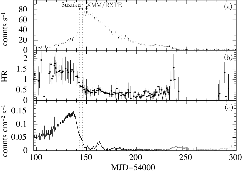
Figure 1: Light curves of GX $339-4$ based on the RXTE/ASM and the Swift/BAT Hard X-ray Transient Monitor. Panel(a) shows the 1.5–12 keV ASM count rate, while panel(b) shows the ASM hardness ratio (5–12 keV/3–5 keV) where data points of large statistic error ($\Delta{\rm HR}>0.7$) are excluded. Panel(c) shows the 15–50 keV BAT count rate. A left-right arrow with vertical dashed lines indicates the time period during which the presented Suzaku data were obtained. Simultaneous observations of XMM and RXTE on 2007 February 19th is indicated with a downarrow.

As described in §1, the 2006/2007 outburst of GX $339-4$ was its brightest outburst since the launch of RXTE in 1995 (Swank et al., 2006). Figure 1 shows the 1.5–12 keV and 15–50 keV light curve and hardness ratio of this outburst, obtained with the RXTE/ASM and the Swift/BAT Transient Monitor. The time histories of the hardness ratio and the Swift/BAT count rate suggests that the state transition occurred around MJD$\simeq$54140–54150. The Suzaku observation was performed on 2007 February 12th 05:33:31 to February 15th 04:48:26 corresponding to MJD=54143.2–54146.2 as indicated with dashed lines in figure 1. Clearly the source hardness and the BAT count rate changed dramatically around the time of the Suzaku observation. An analysis of the QPO seen in RXTE showed a change from type-C to type-B on February 16 (Motta et al., 2009), so the source made a transition from VHS/HIMS to VHS/SIMS between February 15 and 16. The Suzaku spectrum and variability shows this to be a VHS/HIMS spectrum, though there is still an inflection marking the separation of disk and Compton tail (Miller et al., 2008; Yamada et al., 2009).

The XIS employed the 1/4 window option and a burst option (0.3 s for XIS0/XIS1, and 0.5 s for XIS3). The Hard X-ray Detector (HXD; Kokubun et al. 2007) was operated in the standard mode. The data processing and reduction were performed in the same way as Yamada et al. (2009), using the Suzaku pipeline processing version 2.0.6.13. To extract light curves and spectra, the data were analyzed with HEAsoft version 6.9 and the calibration data files (CALDB) released on 2007 July 10th. The XIS events were extracted from a circular region with a radius of 7^′ centered on image peak. Since this extraction circle is larger than the window size of $17^{\prime}.8\times 4^{\prime}.5$, the effective extraction region is therefore the intersection of the window and this circle. As reported in detail by Yamada et al. (2009), the XIS events piled up significantly, and thus a central region of $3^{\prime}$ at the image center was excluded from the event extraction region to minimize these effects. Following Yamada et al. (2009), we use data from XIS0, since data from XIS1 and XIS3 are affected more by pile up than XIS0. In addition, a variable fraction of the CCD frame was often lost due to telemetry saturation, resulting in only 2.83 ks of data out of the 12.4 ks of XIS0 exposure. While Yamada et al. (2009) included data affected by the telemetry saturation to describe the iron line in detail, we excluded the telemetry saturation to avoid a small effect on the continuum shape due to the asymmetric response.

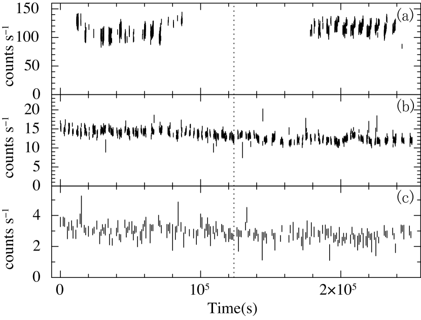
Figure 2: The Suzaku light curves of GX $339-4$ during the observation. Count rate of 0.7–10 keV XIS0 (panel a), 10–60 keV PIN (panel b), and 50–200 keV GSO (panel c) were plotted against time since 2007 February 12th 05:33:31. The XIS0, PIN, and GSO light curves are binned in 6 sec, 100 sec, and 1000 sec, respectively. The XIS0 events within the central region of $3^{\prime}$ were included in panel (a). The PIN and GSO light curves were corrected for dead time, and the NXB was subtracted. A vertical dotted line divided the observation between the first half and the latter half.

The PIN and GSO spectra, acquired for a net exposure of 87.9 ks, were corrected for small dead time, but no other correction due to the source brightness was necessary. We subtracted modeled non-X-ray backgrounds (NXBs; Fukazawa et al. 2009). The PIN and GSO background spectra were constructed based on lcfitdt and lcfit methods (2.0ver0804), respectively, filtered by the same good time intervals. As the response files, ae_hxd_pinxinome3_20080129.rsp was used for PIN, and ae_hxd_gsoxinom_20080129.rsp and ae_hxd_gsoxinom_crab_20070502.arf were used for GSO. The cosmic X-ray background was ignored, since it is less than 1% of the total counts. We use GSO data only up to 200 keV, since the signal becomes smaller than 3% of the background at 200 keV. Figure 2 shows the Suzaku light curves of GX $339-4$ in which background levels were subtracted and dead times were corrected for PIN and GSO data.

4 Analyses of averaged spectrum

In this section, we present the analysis of the Suzaku spectra extracted above. To fit the observed spectra, we use the xspec spectral fitting package(version 12.6.0). We use energy range 0.7–9.0 keV for XIS0, 13–60 keV for the PIN spectrum, and 70–200 keV for the GSO spectrum. Large fit residuals due to calibration uncertainties are often observed near the edge structures of the XIS/XRT instrumental responses so we exclude XIS data from 1.4–2.3 keV. We fit the three spectra simultaneously, with constant factors scaling between the three fixed at 1, 1.07, and 1.07 for XIS, PIN and GSO, respectively. We extend the energy range of the spectral fitting to 0.1–1000 keV as we use some convolution models. Such models have edge effects at the end of the energy range used for the calculation, so it is important that this beyond the energy range used for the data.

4.1 Empirical modeling by diskbb and power-law with reflection (model 1)

In order to characterize the spectral shape, we first model the 0.7–200 keV Suzaku data in the same way as Yamada et al. (2009), i.e., the diskbb model plus power-law (hereafter PL) model. We hereafter call this ‘model 1’. The two continuum components are both absorbed by a common hydrogen column modeled with xspec wabs model (Morrison & McCammon, 1983). While Yamada et al. (2009) used laor model to describe the iron line in detail, we use a single gaussian with $\sigma$ at 0.2 keV since we focus on the continuum shape and our much shorter exposure (due to more stringent constraints on telemetry issues) means that the spectra have much lower statistics.

To account for ionized reflection of the PL component, we utilized the model ireflect (a convolution version of the pexriv model Magdziarz & Zdziarski 1995). This model balances photoionisation with radiative recombination from the very simplistic ionization balance code of (Done et al., 1992). This requires a user defined (rather than self-consistently computed) temperature, which we set to $10^{6}$ K as the disk is clearly hot. However, the code does not calculate collisional processes, so the ion population are set only by photoionisation. This is clearly a poor assumption for such a hot disk. Thus the fairly high ionisation parameter required by Yamada et al. (2009) may be an overestimate of the illuminating flux required. Yet another limitation is that Compton scattering within the disk is not included, which has quite a large effect on the characteristic iron line and edge profile in the reflected emission. Photo-ionization heats the disk photosphere to some fraction of the Compton temperature, so this can be of order $\sim 1$ keV for high ionization parameters. All the line/edge features are produced at an optical depth of around unity, so this means that a third of the photons are Compton scattered by these hot electrons, smearing the sharp line/edge seen in ireflect/pexriv (Ross et al., 1999; Ross & Fabian, 2005). This may mean that the relativistic smearing is overestimated, but we caution that generally spectral parameters are all interrelated, so it may instead distort the observed solid angle, ionization state or iron abundance. Despite these drawbacks, we use this as there are few better alternatives at present. The models at high densities of Ross & Fabian (2007) are not yet public.

We fix the ionization parameter $300~{}{\rm erg~{}cm~{}s^{-1}}$, and fix all abundances other than iron at solar. Hence the only free parameters are the amount of solid angle and the iron abundance. We smear this reflected spectrum by general relativistic effects using rdblur (Fabian et al., 1989). We fix all the parameters of this at characteristic values seen by Yamada et al. (2009), i.e. inner and outer radius $R_{\rm in}^{\rm rdblur}=10R_{g}$, $R_{\rm out}^{\rm rdblur}=10^{5}R_{g}$, inclination angle $i=50^{\circ}$, and power law index of emissivity $\beta=-3$ as our limited data quality do not allow us to constrain them independently.

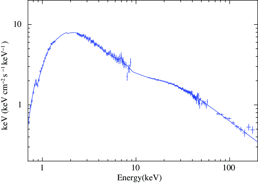
Figure 4: $\nu F_{\nu}$ spectrum of GX$339-4$ from the best fit model 1, where PIN and GSO spectra are normaized to XIS-0 spectrum.

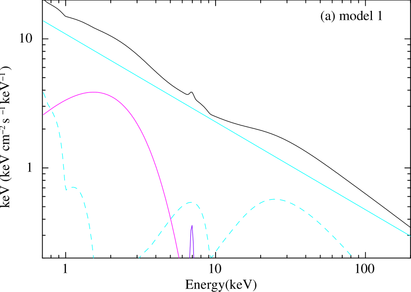
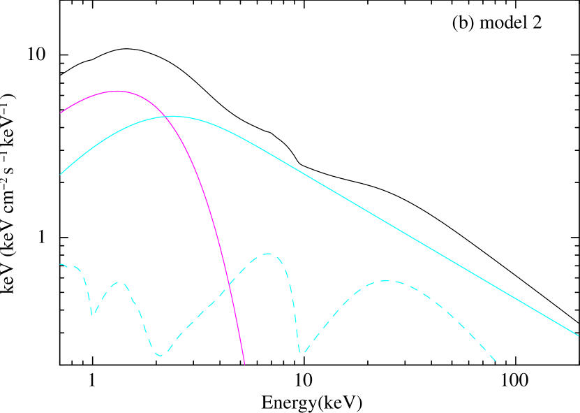
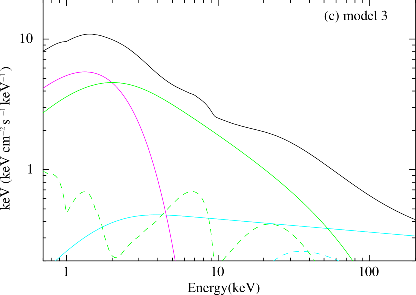
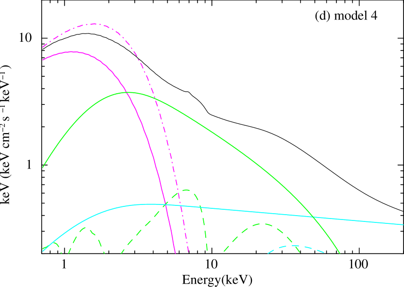
Figure 5: Model spectra of GX$339-4$ from the best fit model 1 (panel a), model 2 (panel b), model 3 (panel c), and model 4 (panel d), where the interstellar absorption is excluded. Emission from the underlying disk (diskbb or dkbbfth(d); magenta), non-thermal compton component (pl or simpl(c); light blue), thermal Compton component (nthcomp or dkbbfth(c); green), and gaussian (purple) are shown solid lines. The reflected components of the thermal (green) and non-thermal (light blue) are shown with dashed lines. In panel (d), the intrinsic disk emission (magenta dash-dot line), where all the power of the dkbbfth component is released as optically thick disk, is plotted together with the original model components.

Table 1 gives details how the model was described in xspec, while Table 2 gives the best fit parameters. This shows that model 1 fits the data well with $\chi^{2}/dof=190.2/186$. Figure 3 shows the data and the best fit model and residuals, while figure 4 and figure 5(a) show the $\nu F_{\nu}$ spectrum and unabsorbed model spectrum, respectively. The absorbed 0.7–200 keV flux is estimated as $2.8\times 10^{-8}~{}{\rm erg~{}s^{-1}cm^{-2}}$ which gives an absorbed luminosity of $2.1\times 10^{38}~{}d_{8}~{}{\rm erg~{}s^{-1}}$ assuming isotropic emission. The PL photon index $\Gamma_{\rm PL}=2.68^{+0.02}_{-0.01}$, so this plus the high luminosity means that the source is in the VHS, as noted by Yamada et al. (2009). The best fit parameters are consistent with those obtained by Yamada et al. (2009) within 90% confidence, and the best fit diskbb model shows disk inner temperature of $kT_{\rm in}=0.65\pm 0.02$ keV and an apparent inner radius of $r_{\rm in}\sim(56^{+5}_{-6})\cdot\zeta_{50}d_{8}$ km, consistent with that observed in the usual HSS, $(52\sim 68)\cdot\zeta_{50}d_{8}~{}{\rm km}$ (see §2).

However, an inspection of the figure 5(a) shows that this is not a good physical description of a model where the disk provides the seed photons for Compton up-scattering into the PL tail as the PL extends below the disk at low energies. This motivates further studies of the disk structure with more physical models.

4.2 Disk geometry based on independent corona (model 2 and model 3)

Compton scattering conserves photon number, so it removes seed photons from the observed spectrum by boosting them in energy to form the Compton tail. We replaced the pl model with a convolution model simpl (Steiner et al., 2009) which self consistently removes as many seed photons as it puts into a Compton tail. This is identified as ‘model 2’ in table 1. As described in table 1, only the up-scattered photons are reflected by the optically thick disk, and thus modified by the models of rdblur and ireflect. The fit results are presented in table 2 and figure 3(c). As shown in unabsorbed model spectrum (figure 5b), this gives a more physical description of the distribution of the low energy photons. The lack of emission at the lowest energies from Comptonization compared to a PL means that the disk temperature becomes lower to compensate for this, with $kT_{\rm in}=0.55^{+0.02}_{-0.01}$ keV, and the radius becomes higher $r_{\rm in}=(122^{+7}_{-8})\cdot\zeta_{50}d_{8}$ km. This implies that the disk inner radius is twice as large as the ISCO, by comparison to that found in the usual HSS.

However, the Comptonization seen in the VHS is complex, containing a mix of both thermal and non-thermal electrons (e.g., Gierliński et al. 1999; Kubota, Makishima & Ebisawa 2001; Gierliński & Done 2003) whereas the simpl model used above only makes a non-thermal power law tail. Hence we added a thermal comptonization model, nthcomp (Zdziarski et al., 1996; Zycki et al., 1999) to the model (model 3 in table 1). This has four parameters, seed disk photon temperature, which we tie to that of the seed photon temperature of diskbb, the electron temperature $kT_{\rm e}$, photon index $\Gamma_{\rm th}$ (equivalent to optical depth), and normalization. The relation between the optical depth, electron temperature and spectral index is given by equation (A1) of Zdziarski et al. (1996) assuming a spherical source with a uniform distribution of seed photons throughout the source. By contrast, we assume slab geometry with seed photons at the bottom of the slab. Comparing these two geometries with compps (geom=$-4$ and 1 respectively, Poutanen & Svensson 1996) shows that the spectral indices are equivalent for an optical depth in the slab geometry which is approximately half that of the sphere. Hence we use

$$\tau=\frac{1}{2}\cdot\left(\sqrt{\frac{9}{4}+\frac{3}{\Theta_{\rm e}\cdot((\Gamma_{\rm th}+\frac{1}{2})^{2}-\frac{9}{4})}}-\frac{3}{2}\right)~{}~{}$$ (1)

where $\Theta_{\rm e}=kT_{\rm e}/m_{\rm e}c^{2}$.

We cannot uniquely constrain both $\Gamma_{\rm th}$ from the thermal Comptonization, and $\Gamma_{\rm pl}$ from simpl so we fix the latter at 2.1, the value of the non-thermal tail seen in the typical HSS (Gierliński et al., 1999). The non-thermal tail may be somewhat steeper in the VHS, and again has a complex shape (Gierliński & Done, 2003). However, our data do not extend above 200 keV so we are not very sensitive to this. Hence model 3 has only two additional free parameters. Similarly to models 1 and model 2, only the Comptonized emission is reflected by the underlying optically thick disk, and thus the model description is somewhat complicated as described in table 1. This gives $\chi^{2}/dof=192.0/184$, still not as good as model 1, but better than model 2. The fits are shown in table 2, figure 3(d) and figure 5(c). These show that the thermal Comptonization dominates the spectrum below $\sim 50$ keV.

Unlike simpl, the thermal Comptonization does not decrease the seed photon spectrum. Hence we have to manually adjust the disk normalization for the photons which are scattered out into the thermal Compton tail. Hence we also tabulate the unabsorbed photon flux $F^{\rm photon}_{\rm th}$ contained in the thermal Compton tail integrated from 0.01-100 keV. We assume that these photons were removed equally from all energies of the disk spectrum (equivalent to a uniform corona over the entire disk). The observed photon flux from the disk, $F^{\rm photon}_{\rm disk}$ is also tabulated, and we simply increase the measured disk normalization by this amount. Since the normalization is proportional to the square root of the radius this gives an inferred radius $r_{\rm in}^{\ast}=r_{\rm in}\sqrt{(F^{\rm photon}_{\rm th}+F^{\rm photon}_{\rm disk})/F^{\rm photon}_{\rm disk}}$, where $r_{\rm in}$ is calculated from the diskbb normalization alone. This is equivalent to equation (A.1) in Kubota & Makishima (2004), and this gives $r_{\rm in}^{\ast}=(117\pm 5)\cdot\zeta_{50}d_{8}$ km, which is as large as that estimated with model 2.

4.3 Inner disk-corona: coupled energetics (model 4)

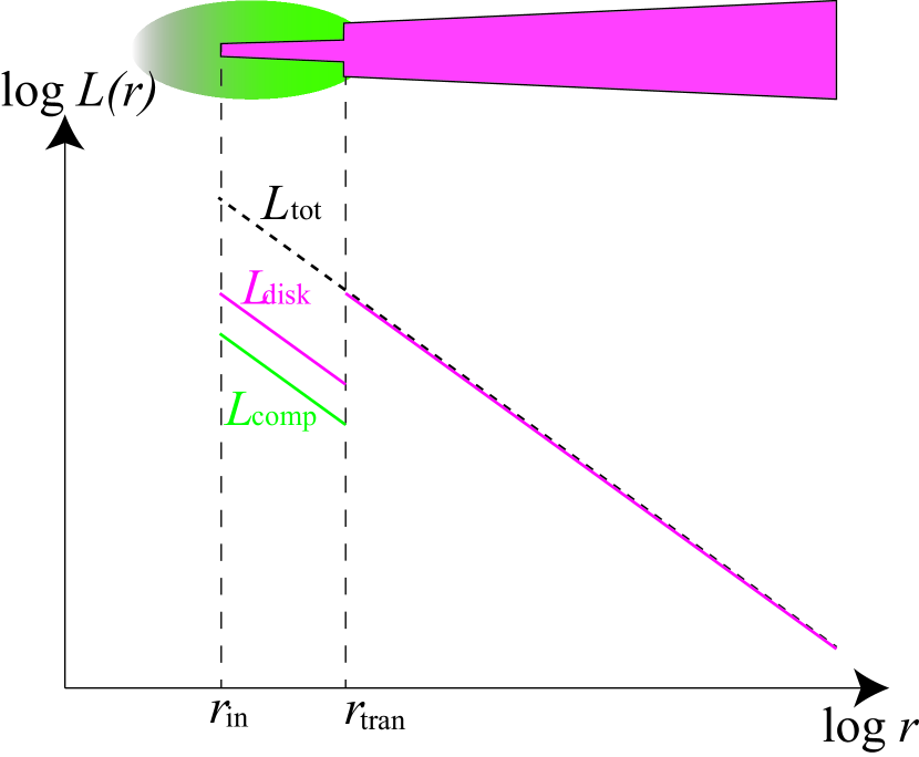
Figure 6: The schematic geometry envisaged for the dkbbfth model. At $r<r_{\rm tran}$, sum of the local luminosity from thermal corona (green) and disk (magenta) are consistent with that expected from the standard disk at $r>r_{\rm tran}$. Details are described in Done & Kubota (2006).

The previous two models assumed that the Comptonizing electrons fully covered the disk, and that the underlying disk structure is unaffected by the presence of the high energy electrons. However, both these assumptions are probably not appropriate. The corona probably only covers the inner disk, at $r_{\rm in}<r<r_{\rm tran}$ as schematically shown in figure 6. The power in the corona must also derive ultimately from the accretion flow, so there should be less power dissipated in the disk.

In the view of these concepts, we fit the data by replacing the ’diskbb+nthcomp’ components in model 3 to the coupled disk-corona model, dkbbfth given by Done & Kubota (2006) (model 4 in table 1). This model assumes that the energy released by gravity is dissipated locally, either thermalising in the disk for $r>r_{\rm tran}$, or split between the disk and corona for $r_{\rm in}<r<r_{\rm tran}$, as shown schematically in figure 6. Thus the disk underlying the corona is cooler and less luminous than it would have been if the corona did not exist, and it is this weak and cool disk emission which provides the seed photons for the Compton upscattering (see Svensson & Zdziarski 1994; Done & Kubota 2006).

The model parameters are similar to that of using a diskbb+nthcomp continuum (model 3), except that rather than having two separate normalizations, the parameters which control the relative normalization of the disk and corona are a combination of $r_{\rm tran}$, which determines the outer, unComptonized disk luminosity, and the shape of the thermal Comptonization i.e. $\Gamma_{\rm th}$ (equivalent to $\tau$) and $kT_{\rm th}$. The luminosity of the Compton component, $L_{\rm th}$, is approximately determined by the Compton $y$ parameter where $y\approx 4\Theta_{e}(\tau+\tau^{2})$ as $L_{\rm th}=yL_{\rm disk,in}$ and $L_{\rm disk,in}$ is the inner disk luminosity for $r_{\rm in}<r<r_{\rm tran}$. Thus the ratio of power dissipated in the corona to that of the disk in the region $r_{\rm in}<r<r_{\rm tran}$ is $f_{\rm th}=L_{\rm th}/L_{\rm disk,in}\approx y$ (see Done & Kubota 2006 for examples of how the model spectra change as a function of these parameters). The inner radius is calculated via equation (A.1) in Kubota & Makishima (2004) by replacing ‘$F_{\rm disk}^{\rm p}+F_{\rm thc}^{\rm p}\cdot 2\cos i$’ to photon flux of the dkbbfth component, $F_{\rm dkbbfth}^{\rm photon}$, assuming the slab geometry. The radius is also determined from the intrinsic (rather than observed) innermost disk temperature, $T_{\rm in}^{\rm int}$. This is how the entire disk would be seen if there was no energy dissipated in the corona.

This model only takes into account the thermal Comptonization, so we again include the simpl with fixed $\Gamma_{\rm PL}=2.1$ to describe the non-thermal tail. In this analysis, we set the un-scattered component of the dkbbfth to be seed photons for simpl. Again, both the thermal (dkbbfth) and non-thermal (simpl) Compton components are both modified by the ionized reflection and blurred by the relativistic effects.

The model has the same number of free parameters as model 3, but gives an improved fit with $\chi^{2}/dof=178.7/184$. This is the best chi-squared value among the four models despite the fact that the model is more constrained. The fit results are summarized in table 2, figure 3(e) and figure 5(d). With the best fit parameters by assuming an isotropic emission, the absorbed and unabsorbed luminosity was estimated in the range of 0.7–200 keV as $(2.1\times 10^{38})d_{8}~{}{\rm erg~{}s^{-1}}$ and $(2.9\times 10^{38})d_{8}~{}{\rm erg~{}s^{-1}}$, respectively. We also calculated the bolometric luminosity $(3.8\times 10^{38})d_{8}~{}{\rm erg~{}s^{-1}}$ and the optical depth of $\tau=0.58^{+0.08}_{-0.07}$ via equation (1). The corona was found to be localized within $r_{\rm tran}$ of $2.7~{}r_{\rm in}^{*}$, within which, 27% of the accretion power is dissipated in the thermal corona.

Considering the power dissipated in the corona, the intrinsic disk temperature should be $kT_{\rm in}^{\rm int}=0.67^{+0.04}_{-0.08}$ keV. With this intrinsic disk temperature and the 0.1–100 keV dkbbfth photon flux of $F_{\rm dkbbfth}^{\rm photon}=43.5~{}{\rm photons~{}s^{-1}cm^{-2}}$, the underlying disk inner radius was estimated as $r_{\rm in}^{\ast}=(93^{+19}_{-8})\cdot\zeta_{50}d_{8}$ km. In figure 5(d), the intrinsic disk emission is plotted together with a dash-dot line. Though the estimated apparent inner radius is slightly smaller than that obtained under the independent corona modeling (model 2 and 3), it is $\sim 1.3$–2.2 times as large as that observed in the HSS (see §2).

We checked that the results were not affected by the assumption that relativistic blurring has a radial dependence parameterized by $\beta=-3$. We replaced this by $\beta=10$, which is more appropriate for a stress-free inner boundary condition by assuming that the line emissivity is proportinal to the local energy release rate in the disk. The difference from the $\beta=-3$ case was negligible. Even removing relativistic effects entirely does not change the continuum parameters significantly due to the limited statistics around the iron line/edge in our data. In all cases the best fit disk parameters were still consistent with those shown in table 2.

5 Is the disk truncated in these data?

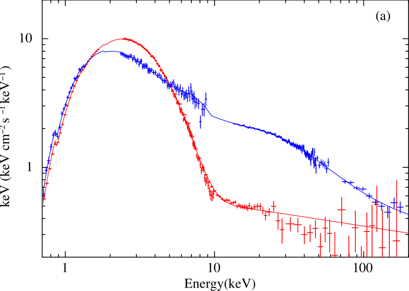
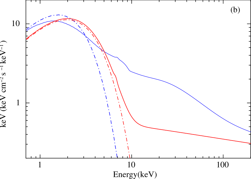
Figure 7: Comparison between the Suzaku averaged spectrum in the VHS/HIMS (blue) and XMM/RXTE spectrum in the HSS obtained on February 19 (red). $\nu F_{\nu}$ spectra and the unabsorbed model spectra by excluding the same interstellar absorption are shown in panel (a) and (b), respectively. A blue dash-dot line indicates the intrinsic disk emission for the Suzaku VHS spectrum in panel (b). The disk emission in the HSS is also indicated with a red dash-dot line.

All the models above which self consistently correct the disk normalization for Compton scattering (models 2, 3 and 4) find a disk inner radius which is larger than that seen in the HSS in this source. This can be seen directly by comparison with a HSS spectrum at a very similar luminosity. Figure 7(a) shows the Suzaku data used here together with the HSS spectrum of almost the same luminosity taken by XMM and RXTE on February 19th (Kolehmainen et al., 2011) (see figure 1). Figure 7(b) shows the comparison of the unabsorbed model spectra.

The HSS spectrum is roughly characterized by a dominant diskbb of $kT_{\rm in}\simeq 0.82$ keV with a weak PL tail, and an absorbed 0.7–200 keV flux is estimated as $2.4\times 10^{-8}~{}{\rm erg~{}s^{-1}cm^{-2}}$, which is only 15% lower than the Suzaku flux of $2.8\times 10^{-8}~{}{\rm erg~{}s^{-1}cm^{-2}}$ in the same energy band. Thus if the disk has constant radius between the HSS and VHS/HIMS then the disk temperature should be slightly higher in the higher luminosity VHS/HIMS. Yet is it clear from this figure that the VHS disk has a lower temperature, as the data peak at lower energy in figure 7(a). Compton scattering retains the imprint of the seed photon energy, so this lower temperature cannot be a consequence of simply Comptonizing the higher temperature inner disk (see Done & Kubota 2006). The blue dash-dot line in figure 7(b) shows the estimated intrinsic disk emission from the VHS/HIMS data as reconstructed from the dkbbfth model, i.e. how the disk emission would have looked in the Suzaku data, if the thermal corona was not present and the matters of thermal corona were all accreted in the disk. If the inner radius is kept constant between the HSS and the VHS/HIMS, the intrinsic disk emission should peak at higher energy than in the HSS. However, the peak energy of the intrinsic disk emission is still much lower than that in the HSS. Estimated intrinsic VHS disk temperature $kT_{\rm in}^{\rm int}=0.67^{+0.04}_{-0.08}$ keV is much lower than the observed HSS disk temperature of $kT_{\rm in}\simeq 0.82$ keV. Therefore, the apparent inner radius of the VHS/HIMS is clearly larger than that in the HSS.

To convert from apparent to true inner disk radius requires corrections for the color temperature, $\kappa$, and inner boundary condition, $\xi$, with $R_{\rm in}=r_{\rm in}\cdot\kappa^{2}\cdot\xi$ as described in §2. If we use the same $\kappa$ and $\xi$, we obtained $R_{\rm in}=(99^{+20}_{-8})\cdot\zeta_{50}d_{8}$ km. Under the same value of $\xi$, the only way to get the same inner radius of the disk in the VHS/HIMS as in the HSS is if $\kappa$ is as low as $\sim 1.3$–1.4. This seems very unlikely given the strong illumination. On the contrary, it is certainly plausible that the disk color temperature correction has increased substantially, as the inner disk should be strongly illuminated by the Comptonized emission in the VHS/HIMS whereas it is not in the HSS. This only reinforces the change in true inner radius as a larger color temperature correction means that $R_{\rm in}$ is even larger than derived from assuming $\kappa=1.7$. Similarly, if the disk in truncated, then the use of the same boundary condition is not appropriate as it now does not extend down to the ISCO, where there is the stress-free inner boundary, but is truncated where there can still be stress on the inner boundary, making $\xi$ larger. This again leads to an increase in $R_{\rm in}$ (see also the discussion in (Gierliński et al., 2008).

Thus both of the expected changes in color temperature and inner boundary condition reinforce the conclusion that the disk inner radius is larger in the VHS/HIMS than in the HSS. Using $\kappa=1.9$ (Shimura & Takahara, 1995) and $\xi=1$ as a reference, $R_{\rm in}$ can be as large as $\sim 340\cdot\zeta_{50}d_{8}$ km.

6 Variability of the disk and corona

6.1 QPO frequency

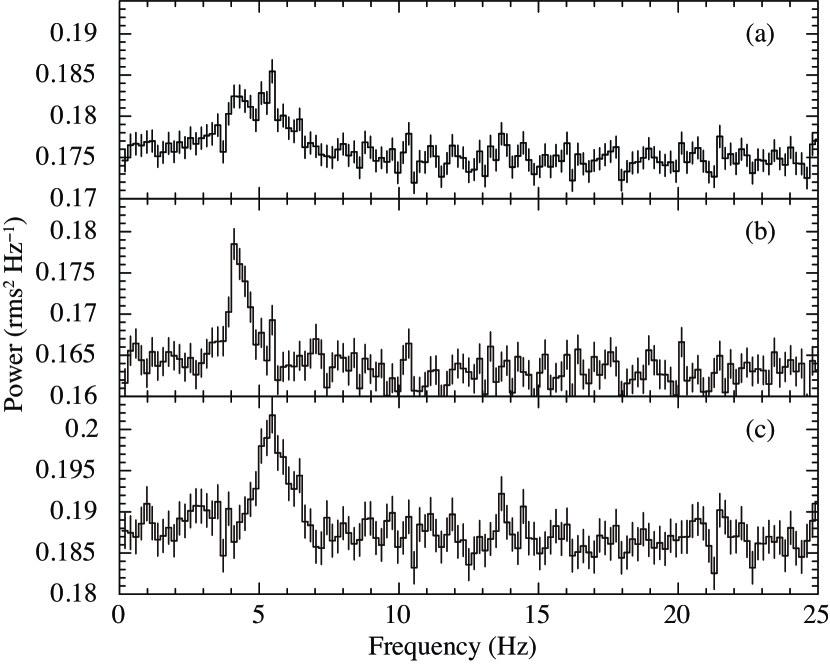
Figure 8: Power spectral density plots calculated based on NXB subtracted PIN lightcurve in the range of 10–60 keV, where white noise level was not subtracted. Panel (a) shows the power spectral density based on the entire light curve, while panel (b) and (c) shows those of the first half and the latter half, respectively.

Figure 8(a) shows the power spectral density from the entire PIN lightcurve calculated using xronos (version5.22). In this figure, a double QPO feature seen at frequencies of $\sim 4$ Hz and $\sim 5$–6 Hz. During the observation, PIN and GSO count rates slightly decreased by $\sim 25$% and $\sim 18$%, respectively, while that of XIS-0 slightly increased $\sim 9$% (figure 2). Thus the double QPO feature is probably due to a change of a single QPO frequency.

We reanalyzed the same data by dividing them into first half and latter half as indicated in figure 2. The calculated power spectral densities were also shown in figure 8(b)(c) showing a clear change in QPO frequency from $4.26\pm 0.06$ Hz in the first half to $5.46\pm 0.06$ Hz, in the second half. Since these QPO frequencies are probably set by the size of the emission region, we look for changes in the size of the disk and corona in their corresponding spectra. Specifically, a higher frequency QPO should indicate a smaller size region, and our modeling with dkbbfth means that we can track both the size of the disk and the size of the corona via the parameters $r_{\rm in}^{*}$ and $r_{\rm tran}$. We then compare the observed changes with the predictions of two specific QPO models.

6.2 Time evolution of spectral parameters

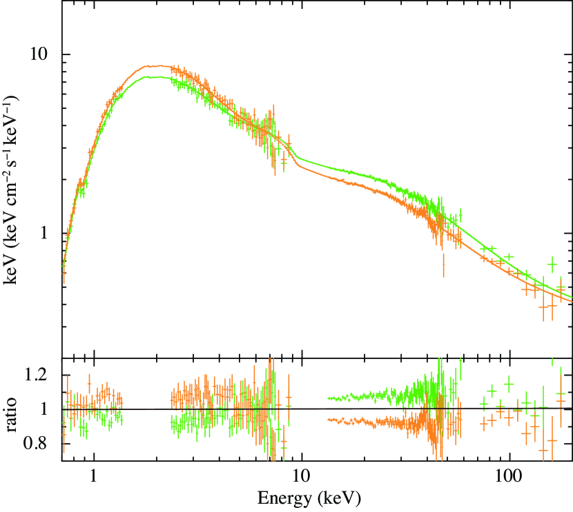
Figure 9: $\nu F_{\nu}$ spectra taken from the first half (green) and the latter half (orange) are plotted in the top panel based on the best fit model 4. The ratios to the best fit model 4 for the summed spectrum are plotted in the same color in the bottom panel.

To investigate evolution of the disk and corona in detail, we accumulated spectra from the two halves of the observation. For PIN and GSO data, net exposures of 43.9 ks and 44.0 ks were acquired for the first half and the latter half, respectively. The NXB spectra were calculated for each periods and subtracted from the data. For XIS0 data, 1.6 ks and 1.3 ks exposures were acquired for the first half and the latter half, respectively. The two data sets have very similar observed luminosities. The absorbed flux was almost same as $2.7\times 10^{-8}~{}{\rm erg~{}s^{-1}cm^{-2}}$ and $2.8\times 10^{-8}~{}{\rm erg~{}s^{-1}cm^{-2}}$, for the first half and the latter half, respectively, while their spectral shape was clearly different. The top panel of figure 9 shows $\nu F_{\nu}$ spectra of the first half (green) and the latter half (orange), and the bottom panel shows ratios of each spectrum to the best fit model 4 for the summed spectrum. There is a clear anti-correlation between the soft band data and the hard band data. The XIS0 data in 1–4 keV increased, while the PIN data decreased, so the spectrum pivots around 10 keV, becoming significantly softer during the Suzaku observation.

A closer inspection of figure 9 reveals that the data below 1 keV do not take part in this spectral pivoting, but remain relatively stable, despite the 10–20 % flux change in the range of 2–4 keV. These photons below $\sim 1$ keV are from the outer part of the disk, where the local temperature is lower than $\sim 0.3$ keV. Since this emission does not change it seems most likely that the mass accretion rate through the disk is not changing (as is also implied by the constant luminosity), and it is only the geometry of the inner disk/corona which gives the spectral change above 1 keV.

In order to discuss change of the spectral parameters, we fit the two data sets with the independent corona (model 3) and the coupled corona (model 4). We fixed the values of $N_{\rm H}$, iron abundance, and the gaussian central energy at those of the best fit values obtained by the summed spectral fit (table 2). Furthermore, in the case of model 4, to avoid a strong coupling between $\tau$ and $kT_{\rm e}$, we fix $kT_{\rm e}$ to the value seen in the average spectrum.

The results are summarized in table 3, and again the energetically coupled corona model dkbbfth gives the best fit. Based on the best fit model 4, the photon index of thermal corona $\Gamma_{\rm th}$ increases from $2.59\pm 0.03$ to $2.74\pm 0.04$. Since we keep $kT_{\rm e}$ constant between the two datasets, this means that the optical depth of the thermal corona $\tau$ slightly decreased from $0.61\pm 0.02$ to $0.55^{+0.02}_{-0.01}$. Hence the second half of the data have a lower $y$ parameter and softer Compton tail, as seen in Figure 9(a). This means that $f_{\rm th}$ also decreases, from 0.30 to 0.25. The unComptonized disk emission is slightly more prominent in the second spectrum, so the transition radius decreases slightly from $r_{\rm tran}=(2.6^{+0.4}_{-0.2})r_{\rm in}^{*}$ to $(2.3^{+0.4}_{-0.2})r_{\rm in}^{*}$.

The intrinsic disk temperature $kT_{\rm in}^{\rm int}$ marginally increases from $0.66\pm 0.03$ keV to $0.69^{+0.02}_{-0.03}$ keV, giving an apparent inner radius of the underlying disk, $r_{\rm in}^{\ast}$ which decreases by $\sim 5\%$ from $(95^{+7}_{-6})\cdot\zeta_{50}d_{8}$ km to $(90^{+6}_{-4})\cdot\zeta_{50}d_{8}$ km. Thus the outer radius of the corona, $r_{\rm tran}$ decreases by $\sim 16\%$ from $250\cdot\zeta_{50}d_{8}$ km to $210\cdot\zeta_{50}d_{8}$ km. Model 3 gave a similar result that the disk inner radius decreased $\sim 5\%$ from the first half to the second half data.

6.3 Discussion on the relation of QPO and the thermal corona

Lense-Thirring precession has been proposed as the origin of the low-frequency QPOs (e.g. Stella & Vietri 1998). This can explain both the frequency and the spectrum of the QPO if the precession is of a hot inner Comptonizing flow rather than the thin disk (Ingram et al., 2009). In this model the QPO frequency $f_{\rm QPO}$ is $f_{\rm QPO}\propto r^{-2.1}$. Thus, a $28\pm 3$% increase in QPO frequency means that the size of the precessing region should decrease by $\sim 11\pm 1$%. Since the precession is a vertical mode, the only part of the corona which can precess in this way is the corona interior to $r_{\rm in}^{*}$ (see the schematic diagram in figure 6). The fits imply that $r_{\rm in}^{*}$ decreases by $\sim 5\pm 8$%, consistent with the Lense-Thirring QPO model.

Another model for the low frequency QPO is that it is a mode of the hot inner flow. Global 3D magnetohydrodynamic (MHD) simulations suggest that the magnetorotational instability (MRI) may lead to the quasi-periodic deformation of a hot inner torus from a circle to a crescent (Machida & Matsumoto, 2008). The frequency in their simulation can be roughly related to the size of the inner torus as $f_{\rm QPO}\propto r^{-3/2}$. So the observed change of QPO frequency requires that the radius change by $\sim 15$%. This is slightly larger than the observed decrease in $r_{\rm in}^{*}$. However, their simulation was for an unconstrained hot flow, i.e. there was no cool disk present. It is not clear how this will change the formation and deformation of such a hot inner torus. So the model is probably consistent within the systematic uncertainty.

7 Summary and conclusions

We have analyzed the Suzaku spectrum of GX $339-4$ in the strongly Comptonized VHS/HIMS. We used a series of models to fit the data, starting with the commonly used ’diskbb plus power-law’ model (model 1). We then use progressively better models of the Comptonization, first assuming that it is non-thermal (model 2) and then allowing it to be both thermal and non-thermal (model 3) as required from previous studies (e.g Zdziarski et al. 2001; Gierliński & Done 2003). The strong Comptonization means that many seed photons from the disk are removed by Compton scattering so the disk luminosity is larger than the directly observed luminosity. This effect increases the apparent radius of the disk, though using proper Comptonization models rather than a power law already increases the disk luminosity and gives an apparent radius which is larger than that seen in the HSS. Our final model couples the disk and corona together (model 4).

Both these models except for model 4 assume that the disk and corona are independent components, yet both ultimately derive from the gravitational energy. Hence our final model is a more physical one where an inner corona reduces the power available for the inner disk. This more physical model gives the best fit to the data, and again requires that the apparent radius of the disk is larger than that seen in the HSS. This increase in apparent size of the disk can be seen directly by comparison with an XMM-Newton/RXTE HSS spectrum at almost the same luminosity taken 3 days after the Suzaku data. This clearly shows that the disk temperature is lower in the VHS/HIMS than in the HSS. The only way that this can be consistent with the same true inner disk radius is if the color temperature correction and/or stress at the inner boundary decreases in the VHS/HIMS. However, it is much more likely that these actually increase, as there is strong irradiation in the VHS/HIMS which should increase the color temperature correction, and it is not possible to decrease the stress on the inner boundary from the zero stress condition used for the HSS. Thus the data show that the VHS/HIMS is associated with a truncated cool disk geometry, where the disk inner radius is 1.3–2.2 times larger than that of the constant radius seen in the HSS which is identified with the ISCO.

Within the Suzaku observation there is a small change in flux and spectral shape, and a corresponding change in the fast variability properties as determined from the power spectrum. The low frequency QPO increases from $4.26\pm 0.06$ Hz to $5.46\pm 0.06$ Hz as the spectrum softens, with a derived decrease in apparent disk inner radius of $r_{\rm in}^{*}=(95^{+7}_{-6})\cdot\zeta_{50}d_{8}$ km to $(90^{+6}_{-4})\cdot\zeta_{50}d_{8}$ km. While this is not significant, this decrease in radius is consistent with the increase in QPO frequency if the QPO is formed either from Lens-Thirring precession of the hot flow interior to $r_{\rm in}$ (Ingram et al., 2009) or from a magneto-hydrodynamic mode of this flow (Machida & Matsumoto, 2008).

A slightly truncated disk in the VHS/HIMS clearly makes a smooth connection to a larger radius disk truncation as required for LHS models which use the alternative hot flow solutions (Esin et al., 1997), making a coherent picture of the outbursts of BHB in a model where the spectrum changes from LHS-VHS/HIMS-HSS driven by a decreasing inner disk radius until it reaches the ISCO.

We would like to thank the referee Dr. Andrzej Zdziarski for his helpful comments. We are grateful to all the Suzaku team members. We also thank Mami Machida and Ryoji Matsumoto for helpful discussion on QPO and MHD. The present work is supported in part by Grant-in-Aid No.19740113 from Ministry of Education, Culture, Sports, Science and Technology of Japan, and by Grant-in-Aid for Project Research in Shibaura Institute of Technology.

Table 1: Description of models in xspec

model	descriptions in xspec
model 1	wabs*(diskbb+rdblur*ireflect*pl + gauss)
model 2	wabs*(simpl(d)*diskbb+rdblur*ireflect* simpl(c)*diskbb+gauss)
model 3	wabs*(simpl(d)*diskbb+rdblur*ireflect*(simpl(c)*diskbb+nthcomp)+gauss)
model 4	wabs*(simpl(d)*dkbbfth(d)+rdblur*ireflect*(simpl(c)*dkbfth(d)+dkbbfth(c))+gauss)

Note. — To use convolution models, simpl, ireflect, and rdblur, energies are extended in the range of 0.1–1000 keV.

Table 2: The best fit parameters for the summed spectrum

Component	Parameter	model 1	model 2	model 3	model 4
wabs	$N_{\rm H}(10^{21}~{}{\rm cm^{-2}})$	$6.7\pm 0.2$	$4.8^{+0.1}_{-0.2}$	$4.9\pm 0.2$	$4.9^{+0.1}_{-0.2}$
diskbb	$kT_{\rm in}$ (keV)	$0.65\pm 0.02$	$0.55^{+0.02}_{-0.01}$	$0.56\pm 0.02$	—
	$r_{\rm in}$ ($\zeta_{50}d_{8}$ km)	$56^{+6}_{-5}$	$122^{+7}_{-8}$	$94^{+6}_{-5}$	—
nthcomp or dkbbfth	$kT_{\rm in}^{\rm int}$ (keV)	—	—	—	$0.67^{+0.04}_{-0.08}$
	$\Gamma_{\rm th}$	—	—	$2.72\pm 0.04$	$2.67^{+0.02}_{-0.03}$
	$kT_{\rm e}$ (keV)	—	—	$72^{+>230}_{-40}$	$41\pm 6$
	norm	—	—	$3.7\pm 0.3$	$1.2\pm 0.3$
	$r_{\rm tran}$ ($r_{\rm in}$)	—	—	—	$2.5^{+0.4}_{-0.2}$
	derived $\tau$	—	—	$0.4\pm 0.3$	$0.58^{+0.08}_{-0.07}$
	derived $f_{\rm th}$	—	—	—	0.27
pl or simpl	$\Gamma_{\rm PL}$	$2.68^{+0.02}_{-0.01}$	$2.68\pm 0.01$	(2.1)	(2.1)
	norm	$11.1\pm 0.5$	—	—	—
	$f_{\rm PL}$	—	$0.33\pm 0.01$	$0.043^{+0.005}_{-0.009}$	$0.032\pm 0.002$
ireflect	$\Omega/2\pi$	$0.79\pm 0.05$	$0.82^{+0.03}_{-0.05}$	$0.83^{+0.07}_{-0.08}$	$0.74^{+0.07}_{-0.07}$
	Fe abundance (solar)	$1.8\pm 0.2$	$1.7\pm 0.2$	$1.8^{+0.4}_{-0.2}$	$1.9^{+0.3}_{-0.2}$
gaussian	E (keV)	$6.94\pm 0.34$	$6.96$	$6.94$	$6.94$
	eqw (eV)	$53^{+46}_{-45}$	$8^{+45}_{-8}$	$5^{+46}_{-5}$	$16^{+43}_{-16}$
	$\chi^{2}/dof$	190.2/186	198.9/186	192.0/184	178.7/184
photon flux	$F_{\rm disk+th}^{\rm photon}~{}({\rm photons~{}s^{-1}cm^{-2}})$	—	—	39.7	43.5
inner radius	$r_{\rm in}^{\ast}$ ($\zeta_{50}d_{8}$ km)	—	—	$117\pm 5$	$93^{+19}_{-8}$

Note. — Errors represents 90% confidence limit of statistical errors. Energy band was extended as 0.1–1000 keV.

Table 3: The best fit parameters of model 3 and 4 for the spectra in the first half and the latter half

Component	Parameter	model3		model4
		first half	latter half	first half	latter half
diskbb	$kT_{\rm in}$ (keV)	$0.54\pm 0.01$	$0.58^{+0.02}_{-0.01}$	—	—
	$r_{\rm in}$ ($\zeta_{50}d_{8}$ km)	$99^{+3}_{-4}$	$91\pm 3$	—	—
nthcomp or dkbbfth	$kT_{\rm in}^{\rm int}$ (keV)	—	—	$0.66\pm 0.03$	$0.69^{+0.02}_{-0.03}$
	$\Gamma_{\rm th}$	$2.63^{+0.03}_{-0.04}$	$2.80^{+0.04}_{-0.05}$	$2.59\pm 0.03$	$2.74\pm 0.04$
	$kT_{\rm e}$ (keV)	$38^{+41}_{-12}$	$>41$	(41)	(41)
	norm	$3.5\pm 0.3$	$3.7^{+0.3}_{-0.4}$	$1.3^{+0.3}_{-0.2}$	$1.2^{+0.1}_{-0.2}$
	$r_{\rm tran}$ ($r_{\rm in}$)	—	—	$2.6^{+0.4}_{-0.2}$	$2.3^{+0.4}_{-0.2}$
	derived $\tau$	$0.6\pm 0.3$	$<0.55$	$0.61\pm 0.02$	$0.55^{+0.02}_{-0.01}$
	derived $f_{\rm th}$	—	—	$0.30$	$0.25$
simpl	$\Gamma_{\rm PL}$	(2.1)	(2.1)	(2.1)	(2.1)
	$f_{\rm PL}$	$0.052^{+0.005}_{-0.006}$	$0.035^{+0.005}_{-0.004}$	$0.035\pm 0.002$	$0.028\pm 0.002$
ireflect	$\Omega/2\pi$	$0.76^{+0.09}_{-0.09}$	$0.88^{+0.11}_{-0.04}$	$0.66^{+0.06}_{-0.08}$	$0.82\pm 0.10$
	Fe abundance (solar)	(1.8)	(1.8)	(1.9)	(1.9)
gaussian	E (keV)	(6.94)	(6.94)	(6.94)	(6.94)
	eqw (eV)	$<49$	$<64$	$<58$	$5^{+66}_{-5}$
	$\chi^{2}/dof$	185.1/184	190.9/184	180.5/185	184.6/185
photon flux	$F_{\rm disk+th}^{\rm photon}~{}({\rm photons~{}s^{-1}~{}cm^{-2}})$	38.7	41.1	43.0	44.3
inner radius	$r_{\rm in}^{\ast}$ ($\zeta_{50}d_{8}$ km)	$122^{+4}_{-5}$	$116^{+3}_{-4}$	$95^{+7}_{-6}$	$90^{+6}_{-4}$

Note. — Same as table 2 but for the separated spectra fit with model 3 and 4.

Figure 3: The Suzaku raw spectra of GX $339-4$, together with predictions of the best-fit model 1 are shown in panel (a). Residuals between the data and model 1, model 2, model 3, and model 4, are shown in panel (b), (c), (d), and (e), respectively.

References

- Belloni et al. (1996) Belloni, T., Mendez, M., van der Klis, M., et al. 1996, ApJ, 472, L107
- Belloni et al. (2002) Belloni, T., Psaltis, D., & van der Klis, M. 2002, ApJ, 572, 392
- Belloni (2010) Belloni, T. M. 2010, Lecture Notes in Physics, Berlin Springer Verlag, 794, 53
- Cowley et al. (2002) Cowley, A. P., Schmidtke, P. C., Hutchings, J. B., & Crampton, D. 2002, AJ, 123, 1741
- Cunningham (1975) Cunningham, C. T., 1975, ApJ, 202, 788
- Done et al. (1992) Done, C., Mulchaey, J. S., Mushotzky, R. F., & Arnaud, K. A. 1992, ApJ, 395, 275
- Done & Kubota (2006) Done, C., & Kubota, A. 2006, MNRAS, 371, 1216
- Done et al. (2007) Done, C., Gierliński, M., & Kubota, A. 2007, A&A Rev., 15, 1
- Dunn et al. (2010) Dunn, R. J. H., Fender, R. P., Körding, E. G., Belloni, T., & Cabanac, C. 2010, MNRAS, 403, 61
- Esin et al. (1997) Esin, A. A., McClintock, J. E., & Narayan, R. 1997, ApJ, 489, 865
- Fabian et al. (1989) Fabian, A. C., Rees, M. J., Stella, L., & White, N. E. 1989, MNRAS, 238, 729
- Fukazawa et al. (2009) Fukazawa, Y., Mizuno, T., Watanabe, S., et al. 2009, PASJ, 61, 17
- Gierliński et al. (1999) Gierliński, M., Zdziarski, A. A., Poutanen, J., et al. 1999, MNRAS, 309, 496
- Gierliński & Done (2003) Gierliński, M., & Done, C. 2003, MNRAS, 342, 1083
- Gierliński et al. (2008) Gierliński, M., Done, C., & Page, K. 2008, MNRAS, 388, 753
- Hynes et al. (2003) Hynes, R. I., Steeghs, D., Casares, J., Charles, P. A., & O’Brien, K. 2003, ApJ, 583, L95
- Hynes et al. (2004) Hynes, R. I., Steeghs, D., Casares, J., Charles, P. A., & O’Brien, K. 2004, ApJ, 609, 317
- Ingram et al. (2009) Ingram, A., Done, C., & Fragile, P. C. 2009, MNRAS, 397, L101
- Kokubun et al. (2007) Kokubun, M., Makishima, K., Takahashi, T., et al. 2007, PASJ, 59, 53
- Kolehmainen & Done (2010) Kolehmainen, M., & Done, C. 2010, MNRAS, 406, 2206
- Kolehmainen et al. (2011) Kolehmainen, M., Done, C., & Díaz Trigo, M. 2011, MNRAS, 416, 311
- Kubota et al. (1998) Kubota, A., Tanaka, Y., Makishima, K., et al. 1998, PASJ, 50, 667
- Kubota, Makishima & Ebisawa (2001) Kubota, A., Makishima, K., & Ebisawa, K., 2001, ApJ, 560, L147
- Kubota & Done (2004) Kubota, A., & Done, C. 2004, MNRAS, 353, 980
- Kubota & Makishima (2004) Kubota, A., & Makishima, K., 2004, ApJ, 601, 428
- Lasota (2001) Lasota, J.-P. 2001, Black Holes in Binaries and Galactic Nuclei, 149
- Magdziarz & Zdziarski (1995) Magdziarz, P., & Zdziarski, A., 1995, MNRAS, 273, 837
- Machida & Matsumoto (2008) Machida, M., & Matsumoto, R. 2008, PASJ, 60, 613
- Makishima et al. (1986) Makishima, K., Maejima, Y., Mitsuda, K., et al. 1986, ApJ, 308, 635
- Markert et al. (1973) Markert, T. H., Canizares, C. R., Clark, G. W., et al. 1973, ApJ, 184, L67
- McClintock & Remillard (2006) McClintock, J. E., & Remillard, R. A. 2006, Compact stellar X-ray sources, 157
- Mendez & van der Klis (1997) Mendez, M., & van der Klis, M. 1997, ApJ, 479, 926
- Miller et al. (2008) Miller, J. M., Reynolds, C. S., Fabian, A. C., et al. 2008, ApJ, 679, L113
- Mitsuda et al. (1984) Mitsuda, K., Inoue, H., Koyama, K., et al. 1984, PASJ, 36, 741
- Miyamoto et al. (1991) Miyamoto, S., Kimura, K., Kitamoto, S., Dotani, T., Ebisawa, K. 1991, ApJ, 383, 784
- Morrison & McCammon (1983) Morrison, R., & McCammon, D. 1983, ApJ, 270, 119
- Motta et al. (2009) Motta, S., Belloni, T., & Homan, J. 2009, MNRAS, 400, 1603
- Muñoz-Darias et al. (2008) Muñoz-Darias, T., Casares, J., & Martínez-Pais, I. G. 2008, MNRAS, 385, 2205
- Ponti et al. (2012) Ponti, G., Fender, R. P., Begelman, M. C., et al. 2012, arXiv:1201.4172
- Poutanen & Svensson (1996) Poutanen, J., & Svensson, R. 1996, ApJ, 470, 249
- Ross et al. (1999) Ross, R. R., Fabian, A. C., & Young, A. J. 1999, MNRAS, 306, 461
- Ross & Fabian (2005) Ross, R. R., & Fabian, A. C. 2005, MNRAS, 358, 211
- Ross & Fabian (2007) Ross, R. R., & Fabian, A. C. 2007, MNRAS, 381, 1697
- Rykoff et al. (2007) Rykoff, E. S., Miller, J. M., Steeghs, D., & Torres, M. A. P. 2007, ApJ, 666, 1129
- Shakura & Sunyaev (1973) Shakura, N., Sunyaev, R., 1973, A&A, 24, 337
- Shidatsu et al. (2011a) Shidatsu, M., Ueda, Y., Nakahira, S., et al. 2011a, PASJ, 63, 803
- Shidatsu et al. (2011b) Shidatsu, M., Ueda, Y., Tazaki, F., et al. 2011b, PASJ, 63, 785
- Shimura & Takahara (1995) Shimura, T., Takahara, F.,1995, ApJ, 445, 780
- Steiner et al. (2009) Steiner, J. F., Narayan, R., McClintock, J. E., & Ebisawa, K. 2009, PASP, 121, 1279
- Steiner et al. (2010) Steiner, J. F., McClintock, J. E., Remillard, R. A., et al. 2010, ApJ, 718, L117
- Stella & Vietri (1998) Stella, L., & Vietri, M. 1998, ApJ, 492, L59
- Svensson & Zdziarski (1994) Svensson, R., & Zdziarski, A. A. 1994, ApJ, 436, 599
- Swank et al. (2006) Swank, J. H., Smith, E. A., Smith, D. M., & Markwardt, C. B. 2006, The Astronomer’s Telegram, 944, 1
- Wijnands et al. (1999) Wijnands, R., Homan, J., & van der Klis, M. 1999, ApJ, 526, L33
- Yamada et al. (2009) Yamada, S., Makishima, K., Uehara, Y., et al. 2009, ApJ, 707, L109
- Zdziarski et al. (1996) Zdziarski, A. A., Johnson, W. N., & Magdziarz, P. 1996, MNRAS, 283, 193
- Zdziarski et al. (2001) Zdziarski, A. A., Grove, J. E., Poutanen, J., Rao, A. R., & Vadawale, S. V. 2001, ApJ, 554, L45
- Zdziarski et al. (2002) Zdziarski, A. A., Poutanen, J., Paciesas, W. S., & Wen, L. 2002, ApJ, 578, 357
- Zdziarski et al. (2004) Zdziarski, A. A., Gierliński, M., Mikołajewska, J., et al. 2004, MNRAS, 351, 791
- Zycki et al. (1999) Zycki, P. T., Done, C., & Smith, D. A. 1999, MNRAS, 305, 231
- Zhang, Cui & Chen (1997) Zhang, S. N., Cui, W., & Chen, W. 1997, ApJ, 482, L155