Quenched Cold Accretion of a Large Scale Metal-Poor Filament due to
Virial Shocking in the Halo of a Massive $z=0.7$ Galaxy

Abstract

Using HST/COS/STIS and HIRES/Keck high-resolution spectra, we have studied a remarkable Hi absorbing complex at $z=0.672$ toward the quasar Q1317+277. The Hi absorption has a velocity spread of $\Delta v=1600$ km s^-1, comprises 21 Voigt profile components, and resides at an impact parameter of $D=58$ kpc from a bright, high mass ($\log M_{\rm vir}/M_{\odot}\simeq 13.7$) elliptical galaxy that is deduced to have a 6 Gyr old, solar metallicity stellar population. Ionization models suggest the majority of the structure is cold gas surrounding a shock heated cloud that is kinematically adjacent to a multi-phase group of clouds with detected Ciii, Civ and Ovi absorption, suggestive of a conductive interface near the shock. The deduced metallicities are consistent with the moderate in situ enrichment relative to the levels observed in the $z\sim 3$ Ly$\alpha$ forest. We interpret the Hi complex as a metal-poor filamentary structure being shock heated as it accretes into the halo of the galaxy. The data support the scenario of an early formation period ($z>4$) in which the galaxy was presumably fed by cold-mode gas accretion that was later quenched via virial shocking by the hot halo such that, by intermediate redshift, the cold filamentary accreting gas is continuing to be disrupted by shock heating. Thus, continued filamentary accretion is being mixed into the hot halo, indicating that the star formation of the galaxy will likely remain quenched. To date, the galaxy and the Hi absorption complex provide some of the most compelling observational data supporting the theoretical picture in which accretion is virial shocked in the hot coronal halos of high mass galaxies.

1. Introduction

It is well accepted that galaxies are intimately linked to the gaseous cosmic web and that the evolution of galaxies is governed in large part by the dissipative response of baryonic gas due to the trade off of cooling and dynamical timescales as it accretes into dark matter halos (e.g., Binney, 1977; Rees & Ostriker, 1977; Silk, 1977; White & Rees, 1978). In general, distinct modes of accretion are believed to operate and the mode is dependent primarily upon the dark matter halo mass (e.g., Birnboim & Dekel, 2003; Dekel & Birnboim, 2006), with some dependence on environment (e.g., Kereš et al., 2005) and on feedback (e.g., van de Voort et al., 2011).

“Hot-mode” accretion is the mechanism in which inflowing gas is shock heated as it is compressed by the hot hydrostatic gas halo. This mode dominates around high mass galaxies, where the dynamical time is shorter than the cooling time. For the most part, the gas accretes into the halo, but not necessarily onto the galaxy itself. “Cold-mode” accretion is the mechanism primarily around low mass galaxies, where the cooling time is shorter than the dynamical time so that hot hydrostatic halos do not form and cold gas accretes directly onto the galaxy. At lower redshifts, as densities decrease, the cooling time is generally longer than dynamical time and the rate of infalling material decreases so that cold mode accretion is a minor channel of accretion onto galaxies (e.g., Kereš et al., 2005; Dekel & Birnboim, 2006), though it remains an important channel for the growth of galaxies at all redshifts (e.g., van de Voort et al., 2011).

A possible third mode is the case in which cold dense filaments can penetrate directly into a hot halo of a massive galaxy. If the conditions are favorable for short cooling times in the filament, then shock heating can be avoided and the filamentary gas can directly accrete onto the galaxy (e.g., Dekel & Birnboim, 2006; van de Voort & Schaye, 2011). However, though cold streams can penetrate the hot atmospheres of massive halos at $z\geq 2$, this process significantly diminishes at lower redshift (e.g., Kereš et al., 2009; Faucher-Giguère et al., 2011), though there is plausible evidence of this process occuring in some $z<1$ galaxies (Kacprzak et al., 2011; Ribaudo et al., 2011; Thom et al., 2011; Kacprzak et al., 2012).

One observable signature of a filament may be a “complex” of Hi absorption with a large velocity spread ($\Delta v>1000$ km s^-1). Alternatively, such Hi absorbing complexes may trace the warm hot intergalactic medium (WHIM), or the intracluster and/or intragroup medium. If an observed Hi absorption complex arises from a filament, it is plausible that the filament may be accreting from the intergalactic medium into a galaxy halo or even directly onto a galaxy. Thus, Hi absorption complexes provide unique astrophysical laboratories for placing constraints on our understanding of the intergalactic medium, and the processes giving rise to extended galaxy halos in the context of dark matter overdensities.

At high redshifts ($z>2$), kinematically extended Hi absorbing complexes were studied by Cowie et al. (1996) with Keck/HIRES spectra. They deduced that these structures were filamentary in nature. At lower redshift ($z<0.22$) Shull et al. (1998), Tripp et al. (2001), Shull et al. (2003), and Aracil et al. (2006a) studied three different Hi complexes with high resolution ultraviolet spectra in which metal lines were detected. For these three complexes, several galaxies were found in the vicinity, suggesting moderate size groups. Each of these studies favored a different scenario of explanation for the physical picture of the Hi complex, including Ovi arising in “nearside/backside” shocked infall into the potential well of the galaxy group (Shull et al., 2003), intragroup gas or an unvirialized filamentary structure through the group (Tripp et al., 2001), and tidally stripped material from one of the nearby galaxies (Aracil et al., 2006a).

The spectrum of the quasar Q1317+277 (TON 153, CSO 0873, J131956+272808, $V=16.0$, $z_{\rm em}=1.017$) exhibits a dramatic $\Delta v>1000$ km s^-1 Hi complex observed in Ly$\alpha$ absorption at $z=0.672$. Several optical and ultraviolet spectra of the quasar are available and have been the focus of this Hi complex and/or the Lyman limit metal-line system at $z=0.660$ (Steidel & Sargent, 1992; Bahcall et al., 1993, 1996; Churchill et al., 2000; Ding et al., 2005; Churchill et al., 2007; Kacprzak et al., 2011; Churchill et al., 2012; Kacprzak et al., 2012). Besides being at intermediate redshift, what is unique to this Hi complex is that it lies at 58 kpc projected from a single bright elliptical galaxy at $z_{\rm gal}=0.6719$ (Churchill et al., 2007).

An analysis of the $z=0.672$ Hi complex was presented in Churchill et al. (2007, hereafter Paper I) based upon HST G160L/G190H FOS spectra (PID 2424, PI: J. N. Bahcall), an HST E230M/STIS spectrum (PID 8672, PI: Churchill), and a Keck/HIRES spectrum of the quasar (see Churchill, 1997). In the FOS spectrum, the Hi complex was found to comprise five components of optically thin Hi absorbing gas, which span a velocity range of $\Delta v=1400$ km s^-1. No metal-lines were clearly detected in the FOS, STIS, and HIRES spectra.

Galaxies at the absorber redshifts were first reported by Steidel, Dickinson, & Persson (1994) as part of the their Mgii absorption-selected galaxy survey. The quantified morphological and spectral properties of these galaxies were presented in Paper I based upon an HST/WFPC2 F702W image (PID 5984; PI: Steidel) of the quasar field and Keck/LRIS spectra of the galaxies. Updated analysis of the galaxies is included in Kacprzak et al. (2011), Churchill et al. (2012), and Kacprzak et al. (2012). In summary, the galaxy at the redshift of the Hi complex has $z_{\rm gal}=0.6719$ and an impact parameter of $D=58$ kpc. It is classified as a late-type E/S0 galaxy. The galaxy at the redshift of the $z=0.660$ absorber, which is a rich metal-line Lyman limit system, has $z_{\rm gal}=0.6610$, an impact parameter of $D=104$, and is an inclined Sab galaxy.

In Paper I, we deduced that the gas in the Hi complex has column densities in the range $14.5\leq\log N({\hbox{{\rm H}\kern 1.00006pt{\sc i}}})\leq 15.5$, temperatures in the range $5.0\leq\log T\leq 5.5$, and upper limits on metallicity in the range $-1.0\leq\log Z/Z_{\odot}\leq-3.0$. We further deduced the complex is consistent with a combination of photo and collisional ionized gas. Based upon expectations of simulations (e.g. Davé et al., 1999), we favored a shock heated structure with chemical enrichment consistent with the high redshift intergalactic medium. Our interpretation was that the Hi complex is a shock heated filamentary structure that originated as a photoionized diffuse phase of gas at high redshift and is accreting in the vicinity of the $z_{\rm gal}=0.6719$ elliptical galaxy.

However, the FOS data did not provide the information required to examine the detailed structure of the kinematic and ionization conditions. Thus, we were unable to constrain the kinematic relationships between the putative shock heated gas, the photo and/or collisionally ionized gas, and the $z_{\rm gal}=0.6719$ galaxy. Such information is critical for examining the physics of gas accretion onto galaxies and for comparing with other observations and with cosmological simulations. For example, Cowie et al. (1996) claim that clustered Ly$\alpha$ lines at $z=3$ are observed to have higher ionization conditions at the velocity extremes and suggest this layered structure is a signature of collapsing structures. While this may be a signature for intergalactic filaments, it is not clear that accretion of a filament into a galaxy potential will yield the same velocity-ionization structure. In theoretical treatment (e.g., Birnboim & Dekel, 2003; Dekel & Birnboim, 2006; Birnboim et al., 2007) and cosmological simulations (e.g., Kereš et al., 2005, 2009; van de Voort et al., 2011; van de Voort & Schaye, 2011) accretion onto massive galaxies is expected to shock heat upon entry into a hot coronal halo, and the resulting kinematic-ionization structure may reflect this very different process.

In order to better study the Q1317+277 Hi complex at $z=0.672$, we have obtained a high resolution $R=18,000$ HST/COS spectrum of the quasar, with focus on the Hi Lyman series lines and Ovi $\lambda\lambda 1031,1037$ absorption. We further improved our knowledge of the star formation history, age, and mass of the $z_{\rm gal}=0.6719$ galaxy by obtaining multi-band imaging of the quasar field. Our motivations include (1) a thorough examination of the kinematic, ionization, and chemical structure of the Hi complex, (2) a direct comparison with the galaxy properties to help place the galaxy-absorber system in the context of galaxy evolution scenarios predicted by theories and cosmological simulations for an improved interpretation, and (3) examination whether there is a connection between the $z=0.672$ Hi complex and the galaxy-absorber pair at $z=0.661$, perhaps in the form of “bridge” of weak Ly$\alpha$ absorption between the galaxies.

The paper is structured as follows: Reduction and analysis of the imaging and spectroscopic data are presented in § 2. Our analysis of the galaxy images is presented in § 3 and our analysis of the absorption line data is presented in § 4. In § 5 and § 6, we present our ionization modeling and resulting constraints on the physical conditions of the absorbing gas. We discuss and interpret the data and our findings in § 7. We provide brief a conclusion in § 8. Throughout this work, we assume the cosmological parameters $\Omega_{\Lambda}=0.7$, $\Omega_{m}=0.3$, $\Omega_{k}=0$, and $h=H_{0}/(100~{}\hbox{\hbox{km~{}s${}^{-1}$}}~{}{\rm Mpc}^{-1})=0.7$ (based on Jarosik et al., 2011).

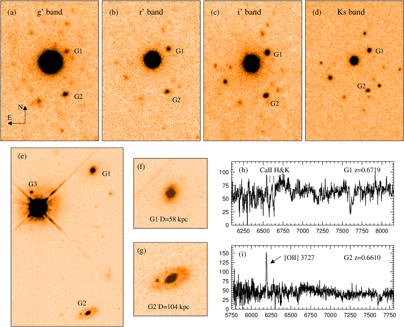
Figure 1.— Images of the quasar field and spectra of the absorbing galaxies. — ($a$–$c$) The $43{\arcsec}\times 60{\arcsec}$ sections of the ground-based APO/SPIcam images centered on the quasar through the SDSS $g^{\prime}$, $r^{\prime}$, $i^{\prime}$ filters. Galaxies G1 and G2 are identified. — ($d$) A $43{\arcsec}\times 60{\arcsec}$ section of the KPNO/IRAM NICMOS image through the $K_{s}$ filter. — ($e$) A $12{\arcsec}\times 22{\arcsec}$ section of the HST/WFPC2 image. Galaxies G1 and G2 are labeled. Also identified and labeled is object G3, a compact galaxy (with unknown redshift) at angular separation $2.1{\arcsec}$ in the north by north-east direction from the quasar. — ($f$) A $4{\arcsec}\times 4{\arcsec}$ view of galaxy G1 at $D=58$ kpc from the quasar. — ($g$) A $4{\arcsec}\times 4{\arcsec}$ view of galaxy G2 at $D=104$ kpc from the quasar. — ($h$) The Keck/LRIS spectrum (counts versus wavelength) of G1, yielded $z_{\rm gal}=0.6719$ from the Caii H&K doublet. — ($i$) The Keck/LRIS spectrum (counts versus wavelength) of G2, yielded $z_{\rm gal}=0.6610$ from the [Oii] $\lambda 3727$ emission line.

2. Observations, Reductions, and Calibrations

We have acquired new data on the $z=0.660$ and $z=0.672$ absorption and the two galaxies G1 and G2. First, we obtained a cycle-17 $R\simeq 18,000$ COS spectrum (PID 11667; PI: Churchill) of the quasar covering the transitions examined in the FOS spectra. Our goals include measuring higher detection sensitivities and detailed kinematics of the absorption lines. Second, we obtained $g^{\prime}$, $r^{\prime}$, $i^{\prime}$, and $K_{s}$ ground-based images of the quasar field. The multi-band images provide colors from which galaxy stellar populations, metallicities, and masses can be estimated.

2.1. Ground-based Images

As part of a larger campaign for imaging Mgii absorption galaxies, we obtained $g^{\prime}$, $r^{\prime}$, $i^{\prime}$ band images of the quasar field using the Seaver Prototype Imaging camera (SPIcam) on the Apache Point Observatory’s (APO) 3.5-m telescope. The detector is a $2048\times 2048$ CCD with 24 $\mu$m pixels, giving an unbinned plate scale of 0.14″ pixel^-1 and a field of view of $4.78{\arcmin}\times 4.78{\arcmin}$. We binned the CCD $2\times 2$ during readout for a plate scale of 0.28″ pixel^-1. Multiple $g^{\prime}$, $r^{\prime}$, and $i^{\prime}$ band images were obtained on the nights of 2006 March 24-25, for which the seeing varied between 1.2-1.5″, and additional $g^{\prime}$ band images were obtained the night of 2007 March 15 for which the seeing was 0.7″. The total summed exposure times are 5190, 4630, and 4350 seconds for the $g^{\prime}$, $r^{\prime}$, and $i^{\prime}$ filters, respectively.

Each frame was reduced using standard IDL and IRAF scripts and tasks. Flat fielding incorporated a combination of dome and sky flats. Cosmic rays were removed in each individual frame. The astrometry was calibrated by position matching of USNO A2.0 stars in the field. Final images were obtained by coadding the individual calibrated frames.

The photometric zero points were obtained using stars in SDSS images. Color terms are required because the filter plus detector throughput of the APO facility is not identical to that of the SDSS facility. These color terms, which are of order 0.1, were determined from SPIcam and SDSS images of roughly 30 quasar fields from our more extensive database.

The near-infrared band images were obtained on 1994 February 24 using the Kitt Peak Mayall 4-m telescope through the $K_{s}$ filter (1.99–2.32 $\mu$m) with the IRIM NICMOS III $256\times 256$ array camera. These images were obtained as part of the campaign culminating in the work of Steidel et al. (1994). The field of view is $154\arcsec\times 154\arcsec$ with plate scale of $0.6\arcsec$ pixel^-1. The NICMOS images were reduced using the contributed IRAF package DIMSUM. Updated photometric zero points were determined using stars from the 2MASS point-source catalog (Strutskie et al., 2006).

All photometric measurements were conducted using SExtractor (Bertin & Arnouts, 1996); we adopted the AUTOMAG results. The dust maps of Schlegel et al. (1998) were used to correct for Galactic dust extinction.

In Figures 1$a$-1$d$, we present $43{\arcsec}\times 60{\arcsec}$ sections of the ground-based images centered on the quasar Q1317+277. A $12\arcsec\times 22\arcsec$ section of the HST/WFPC2 F702W image is presented as Figure 1$e$. Galaxies G1 and G2 labeled in all images. In the HST image, note the object to the north by north-east within 2.1″ of the quasar. We have no estimate of the redshift of this object, which we label G3. Reduction and analysis of the F702W image was described in Paper I, Kacprzak et al. (2011), and Churchill et al. (2012). Expanded views of the two galaxies are presented in Figures 1$f$ and 1$g$. The Keck/LRIS spectra of galaxies G1 and G2 (originally described in Paper I) are presented in Figures 1$h$ and 1$i$. The G1 galaxy redshift was determined using Gaussian centroiding to the Caii absorption features and the redshift of G2 was determined using Gaussian centroiding to the [Oii] $\lambda 3727$ emission line.

2.2. HST/COS spectrum

We obtained a cycle-17 $R\simeq 18,000$ COS spectrum (PID 11667; PI: Churchill) of the quasar covering the transitions first examined in the FOS spectra. Two NUV/G185M spectra were obtained 2010 May 26 and optimally co-added. The first was centered at 1921 Å for a 5420 sec exposure, and the second was centered at 1941 Å for a 4970 sec exposure. The overlap region was 2223–2037 Å on Stripe C, which provided a total of 10,390 sec of integration on the the Hi absorption complex. The FUV/G160M spectrum was obtained 2010 June 26 centered at 1600 Å for an 12,580 sec exposure.

The spectra were reduced following the procedures outlined by Shaw et al. (2009). We continuum fit the lower order shape of the spectrum using the IRAF sfit task and refined the higher order continuum features using our own code Fitter (Churchill et al., 2000).

For the $z=0.660$ and $z=0.672$ absorbers, the Ly$\beta$ and Ly$\gamma$ absorption lines were captured in the NUV on Segment A, the Ly$\delta$ was not captured (fell between segments), and the higher order Lyman series lines were captured on Segment B.

3. Image Analysis: Galaxy Properties

A re-analysis of the HST/WFPC2 F702W image was undertaken, presented, and fully described by Churchill et al. (2012). We adopt the measured quantities from that work.

The G1 quasar-galaxy impact parameter is $D=58$ kpc. The galaxy photometric properties are $M_{B}=-21.6$, $M_{K}=-23.0$, and $B-K=1.4$ (AB). The $B$-band luminosity is $L_{B}/L_{B}^{\ast}=1.28$, where we use $M_{B}^{\ast}$ from the fit with redshift reported by Faber et al. (2007). From an analysis using GIM2D (Simard et al., 2002), we measure a half-light radius of $r_{h}=4.2$ kpc, disk scale length of $r_{d}=0.9$ kpc, and bulge-to-total ratio of $B/T=0.99$. The galaxy classifies as an E/S0 based upon its C-A morphology (Abraham et al., 1996). The galaxy inclination is $i=15.9^{\circ}$, and the angle between the quasar sight line and the major-axis of the projected ellipse of the galaxy is $\theta=22.1^{\circ}$. For the properties of galaxy G2, see Churchill et al. (2012) and our companion paper (Kacprzak et al., 2012).

Photometric analysis of the ground-based images yielded dust-, color-, and seeing-corrected AB apparent magnitudes for galaxy G1 of $m_{g^{\prime}}=23.4\pm 0.03$, $m_{r^{\prime}}=22.2\pm 0.03$ $m_{i^{\prime}}=21.01\pm 0.03$ and $m_{K_{s}}=19.4\pm 0.1$. A color composite image of the ground-based images can be viewed in our companion paper (Kacprzak et al., 2012), from which it can be ascertained that galaxy G1 is clearly redder than galaxy G2 and that the other galaxies in field (see Figures 1$a$-1$d$) are likely at substantially different redshifts.

For galaxy G3, we measured an F702W apparent magnitude of $m=23.4\pm 0.2$. This value is based upon a dithered co-added image constructed by A. Shapley, in which she removed the quasar via point spread function (PSF) subtraction. The quoted uncertainty is statistical based upon the sky background; due to the PSF subtraction, the error could be substantially underestimated. Assuming galaxy G3 is at the redshift of the Hi absorption complex, i.e., $z\simeq 0.672$, and adopting the quoted apparent magnitude, we compute $M_{B}=-19.3$ ($L_{B}/L_{B}^{\ast}=0.16$) and $M_{r}=-20.7$ (SDSS $r$-band). At this redshift, the impact parameter to G3 is $D=14.6$ kpc.

In Figure 2, we plot the $g^{\prime}\!-r\!^{\prime}$ colors versus $i^{\prime}\!-\!K_{s}$ colors for G1 and G2. Following Bell et al. (2003), Fontana et al. (2004), and Swindle et al. (2011), we used stellar population models to determine stellar masses, $M_{\ast}$, of galaxies G1 and G2 from the observed colors. We employed the stellar population models of Bruzual & Charlot (2003) assuming a Chabrier (2003) initial mass function and an exponential star formation history with an $e$-folding time of 1 Gyr. Also shown in Figure 2 are the locust of observed colors as a function redshift for the Bruzual & Charlot (2003) stellar population models for the metallicities $[\hbox{Z/H}]=-0.4$, $0.0$, and $+0.4$. We find galaxy G1 is consistent with a $\simeq 5.8$ Gyr old, solar metallicity stellar population with a formation epoch of $z=4$. The stellar population models also yield the galaxy $K$-band mass to light ratio, $(M/L)_{\hbox{\tiny$K$}}$. From this ratio and the $K$-band magnitude, we estimate $\log M_{\ast}/M_{\odot}=\log(M/L)_{\hbox{\tiny$K$}}-0.4(M_{K}-M_{K,\odot})=11.5$ for galaxy G1, where $M_{K,\odot}=-3.28$ is the solar value.

Using the technique of halo abundance matching, the galaxy virial mass, $M_{\rm vir}$, can be estimated from the stellar mass (e.g., Conroy & Wechsler, 2009; Behroozi, Conroy, & Wechsler, 2010; Moster et al., 2010; Stewart, 2011). Abundance matching assumes a monotonic functional relation between $M_{\rm vir}$ and $M_{\ast}$ by assigning the number of halos with $M_{\rm halo}>M_{\rm vir}$ equal to the number of galaxies with $M_{\rm gal}>M_{\ast}$. As such, it matches the halo mass and stellar mass functions globally with a roughly 0.25 dex uncertainty in $M_{\rm vir}$ at fixed $M_{\ast}$, primarily due to the systematics in estimates of $M_{\ast}$ (Behroozi et al., 2010). We employed the parameterized functions presented by (Stewart, 2011).

Table 1Galaxy Properties

Property	G1	G2	G3
$M_{\rm\ast}/M_{\odot}$	$3\times 10^{11}$	$1\times 10^{11}$	$1\times 10^{10}$
$M_{\rm vir}/M_{\odot}$	$5\times 10^{13}$	$8\times 10^{12}$	$8\times 10^{11}$
$T_{\rm vir}$, K	$1\times 10^{7}$	$3\times 10^{6}$	$7\times 10^{5}$
$v_{\rm circ}$, km s-1	550	280	150
$R_{\rm vir}$, kpc	750	380	180
$M_{\rm gas}/M_{\odot}$	$2\times 10^{10}$	$1\times 10^{10}$	$7\times 10^{9}$
$M_{\rm bary}/M_{\odot}$	$3.2\times 10^{11}$	$1.1\times 10^{11}$	$1.7\times 10^{10}$
$f_{g}$	0.05	0.09	0.34

For galaxy G1, we obtained $M_{\rm vir}=10^{13.7\!-\!14.4}$ M_⊙, where the lower value is given by the Conroy & Wechsler (2009) and Moster et al. (2010) fits and the higher value is from the Behroozi et al. (2010) fit. We adopted the Conroy & Wechsler (2009) and Moster et al. (2010) values $M_{\rm vir}=10^{13.7}$ M_⊙.

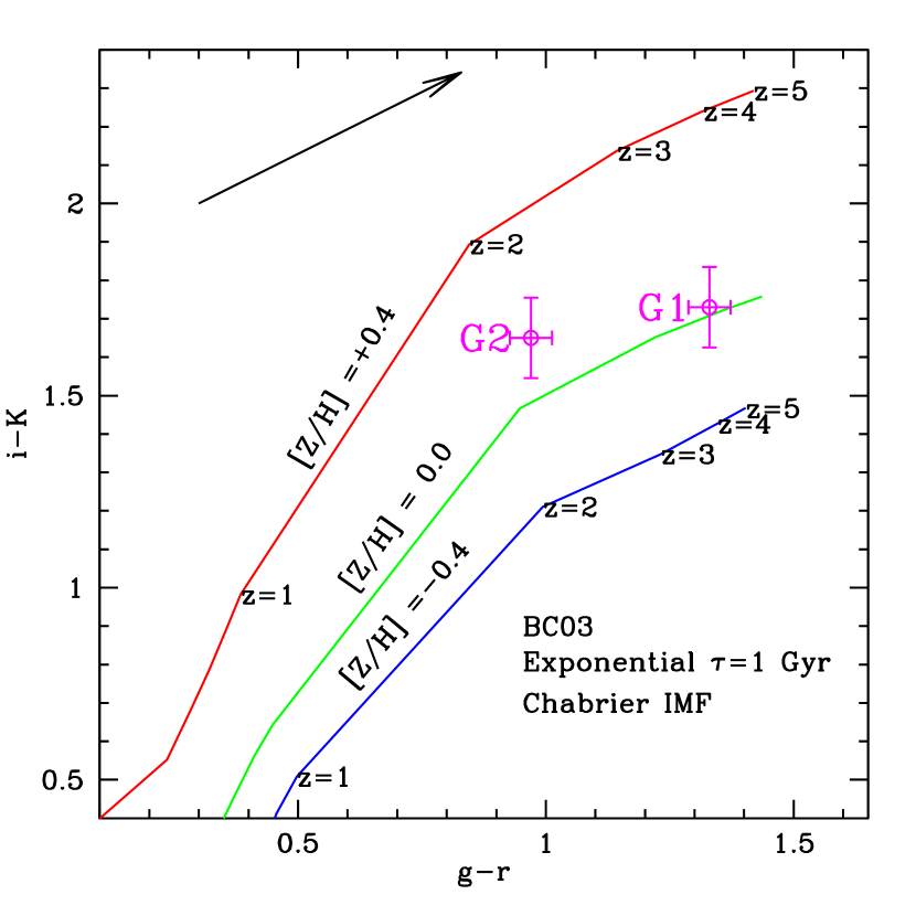
Figure 2.— The $g^{\prime}\!-\!r^{\prime}$ versus $i^{\prime}\!-\!K_{s}$ color-color diagram showing the measured dust-corrected colors of galaxy G1 and G2. The curves are Bruzual & Charlot (2003) stellar population models for metallicities $[\hbox{Z/H}]=-0.4$, $0.0$, and $+0.4$ assuming an exponential star formation rate with an $e$-folding time of 1 Gyr, and a Chabrier (2003) initial mass function. The arrow provides the reddening vector for $E(B\!-\!V)=0.1$ in the rest frame of the galaxies.

Under the assumption that galaxy G3 resides at $z=0.672$, we use the $\Lambda$CDM Bolshoi Simulation Database of Trujillo-Gomez et al. (2011) to estimate a virial mass of $M_{\rm vir}=10^{11.9}$ M_⊙ using abundance matching. This mass is the average of 18,500 galaxies in the absolute magnitude bin $-21.7\leq M_{r}\leq-19.7$ with average $M_{r}=-20.7$. The abundance matching in this database is constrained by the observed luminosity-circular velocity relation, the baryonic Tully-Fisher relation, and the circular velocity function, allowing all types of galaxies to be included. Using the parameterized abundance matching function for $M_{\ast}(M_{\rm vir},z)$ of (Moster et al., 2010), we estimate that G3 has a stellar mass of $M_{\ast}\simeq 10^{10.2}$ M_⊙.

The average gas mass, $M_{\rm gas}$, of a galaxy with stellar mass $M_{\ast}$ can be estimated using the parameterized relation of Stewart (2011) based upon the baryonic Tully-Fisher relation study of McGaugh (2005), the stellar, gas, and dynamical mass relation of Erb et al. (2006), and galaxy gas fraction stellar mass study of Stewart et al. (2009). We obtain $M_{\rm gas}=10^{10.2\!\pm\!0.2}$ M_⊙ for galaxy G1 and estimate $M_{\rm gas}=10^{9.9\!\pm\!0.3}$  M_⊙ for G3. Thus, we deduce averaged baryonic gas fractions, $f_{g}=M_{\rm gas}/(M_{\ast}+M_{\rm gas})$, of 5% for G1 and 34% for G3.

The virial radii, virial temperatures, and circular velocities for galaxies G1 and G3 were computed using the relations of Bryan & Norman (1998) for $\Omega_{\hbox{\tiny R}}=0$. For galaxy G1, we obtained $R_{\rm vir}=750$ kpc, $T_{\rm vir}=1\times 10^{7}$ K, and $v_{\rm circ}=550$ km s^-1 and for galaxy G3, we obtained $R_{\rm vir}=180$ kpc, $T_{\rm vir}=7\times 10^{5}$ K, and $v_{\rm circ}=150$ km s^-1. In Table 1, we summarize the deduced galaxy properties, which are representative averages for galaxies with their observed photometric properties.

4. Spectral Analysis: Absorption Properties

In the FOS spectrum, a very broad Hi absorption complex was observed (first reported by Bahcall et al., 1993). In Paper I we fitted the Ly$\alpha$ with five Gaussian components at redshifts $z=0.66914$, 0.67157, 0.67355, 0.67559, and 0.67707, respectively. The total rest-frame equivalent width was determined to be $W_{r}({\hbox{{\rm Ly}\kern 1.00006pt$\alpha$}})=2.87$ Å over a rest-frame velocity spread of 1420 km s^-1. From the STIS spectrum, the $3~{}\sigma$ Civ $\lambda 1548$ equivalent width limit was estimated to be $W_{r}(1548)\leq 0.03$ Å at $z=0.6719$. In the FOS spectrum, the $3~{}\sigma$ Ovi $\lambda 1031$ equivalent width limit was estimated to be $W_{r}(1031)\leq 0.21$ Å. For Mgii $\lambda 2796$ in the HIRES spectrum, we obtained $W_{r}(2796)\leq 7$ mÅ to $3~{}\sigma$. These values assumed unresolved absorption.

For this work, we objectively locate absorption lines or place limits on their equivalent widths employing the optimized methods of Schneider et al. (1993) and Churchill et al. (1999b) as modified using the methods for unresolved lines and pattern noise developed by Lawton et al. (2008). We adopt a $5~{}\sigma$ detection threshold and quote $3~{}\sigma$ limits.

4.1. Neutral Hydrogen Lines

In Figure 3, we present the Ly$\alpha$, Ly$\beta$, Ly$\gamma$, Ly$\epsilon$, and Ly$\zeta$ absorption observed in the COS spectrum as a function of rest-frame velocity relative to the $z_{\rm gal}=0.6719$ galaxy. No Hi absorption was detected for Lyman series lines higher than Ly$\zeta$. There is significant blending in the Ly$\beta$, Ly$\gamma$, Ly$\epsilon$, and Ly$\zeta$ lines, which are identified in Figure 3, when possible.

The curves through the data are $\chi^{2}$ minimized Voigt profile (VP) fits obtained using our code MINFIT (Churchill, 1997; Churchill & Vogt, 2001; Churchill et al., 2003). The ticks above the normalized continuum provide the VP component velocities. During the fitting, the COS instrumental line spread function (ISF) was convolved with the VP model. The COS ISF appropriate for the spectrograph settings and the observed wavelength of each transition was determined via interpolation of the on-line tabulated data (cf., Dixon et al., 2010; Kriss, 2011).

For the VP fitting, pixels compromised by blending were masked out of the least-squares fit vector. We present the results of our VP modeling in Table 2. We fitted a total of 21 components, or “clouds” (MINFIT returns the minimum number of components based upon their statistical significance through a series of F-tests and confidence level checks). Assuming thermal broadening, we converted the Doppler $b$ parameter into the “cloud” temperature.

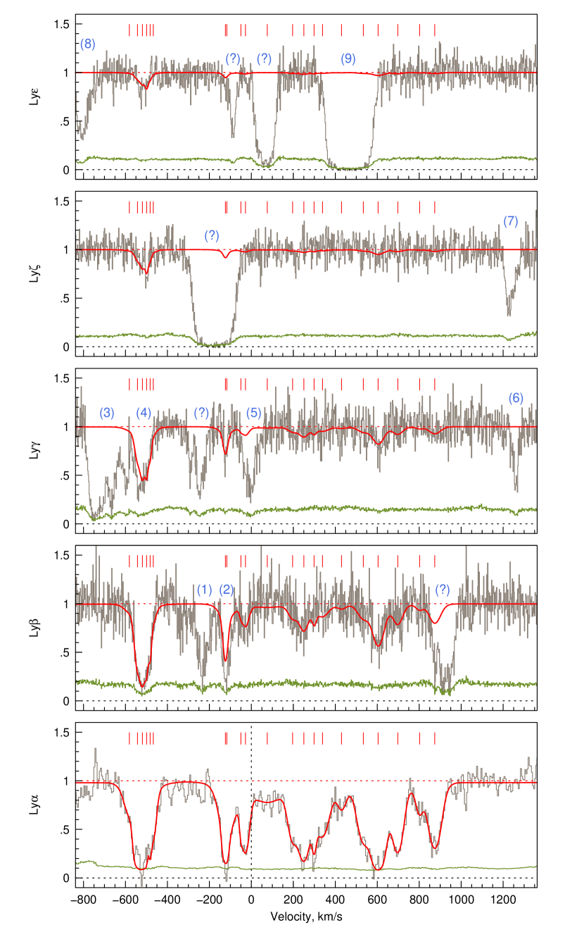
Figure 3.— Voigt profile decomposition of the Hi complex, including Ly$\beta$, Ly$\gamma$, Ly$\zeta$, and Ly$\epsilon$ (Ly$\delta$ was not captured). The vertical dashed line is the redshift of galaxy G1. The component parameters centroids are marked by ticks above the continuum and the fitted component parameters are listed in Tables 2 and 3. Several blends are present and identified as: (1,2) Ovi $\lambda 1031$ associated with the $z=0.6610$ metal system; (3,4) Ciii $\lambda 977$ at $z=0.6610$; (5) Ly$\delta$ at $z=0.7738$; (6) Ciii $\lambda 977$ from clouds #7 & #8 of the Hi complex; (7) Ly$\beta$ $z=0.5349$; (8) Galactic Civ $\lambda 1550$; (9) Ly$\zeta$ at $z=0.6610$. Those marked with “(?)” may well be Ly$\alpha$ lines in that there is no corroborating data to suggest they are metal lines nor higher order Lyman series lines.

Table 2Voigt Profile Decomposition of the Hi Complex

Cld#	$z_{cl}$	$v_{cl}$	$\log N({\hbox{{\rm H}\kern 1.00006pt{\sc i}}})$	$b({\hbox{{\rm H}\kern 1.00006pt{\sc i}}})$	$T$
		[km s-1]		[km s-1]	[$10^{3}$ K]
1	0.668645	$-582.1$	$13.24\pm 0.59$	$31.9\pm 31.3$	$62.0\pm 60.9$
2	0.668861	$-543.5$	$14.26\pm 0.54$	$14.7\pm 9.9$	$13.2\pm 8.9$
3	0.669000	$-518.6$	$14.53\pm 0.33$	$12.8\pm 10.7$	$10.0\pm 8.4$
4	0.669112	$-498.5$	$14.51\pm 0.14$	$3.2\pm 2.1$	$0.6\pm 0.4$
5	0.669199	$-482.9$	$14.07\pm 0.20$	$4.0\pm 1.8$	$1.0\pm 0.4$
6	0.669290	$-520.6$	$13.38\pm 0.38$	$15.5\pm 11.2$	$14.7\pm 10.5$
7	0.671203	$-123.8$	$14.13\pm 0.10$	$11.5\pm 2.9$	$8.1\pm 2.0$
8	0.671244	$-116.6$	$13.69\pm 0.14$	$43.3\pm 14.4$	$114.5\pm 38.1$
9	0.671617	$-49.6$	$12.93\pm 0.94$	$5.8\pm 15.5$	$2.1\pm 5.5$
10	0.671739	$-27.7$	$13.70\pm 0.20$	$18.3\pm 7.7$	$20.5\pm 8.6$
11	0.672319	$+76.1$	$13.43\pm 0.19$	$88.6\pm 49.2$	$479.3\pm 266.1$
12	0.672994	$+197.0$	$13.59\pm 0.28$	$26.4\pm 11.9$	$42.5\pm 19.2$
13	0.673291	$+250.3$	$13.93\pm 0.14$	$27.6\pm 10.9$	$46.4\pm 18.3$
14	0.673562	$+289.9$	$13.38\pm 0.26$	$10.5\pm 6.9$	$6.7\pm 4.4$
15	0.673787	$+339.1$	$13.68\pm 0.15$	$38.4\pm 14.1$	$89.9\pm 33.0$
16	0.674297	$+430.5$	$13.11\pm 0.12$	$26.1\pm 10.1$	$41.6\pm 16.1$
17	0.674872	$+533.5$	$13.70\pm 0.13$	$34.6\pm 8.8$	$73.0\pm 18.6$
18	0.675272	$+605.1$	$14.26\pm 0.05$	$33.7\pm 4.2$	$69.4\pm 8.6$
19	0.675789	$+698.8$	$13.82\pm 0.04$	$29.0\pm 3.4$	$51.5\pm 5.9$
20	0.676366	$+801.2$	$13.10\pm 0.12$	$20.5\pm 7.9$	$25.7\pm 9.9$
21	0.676776	$+874.7$	$13.86\pm 0.04$	$33.5\pm 3.6$	$68.3\pm 7.3$

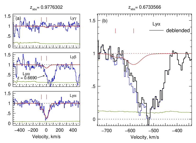
Figure 4.— ($a$) The Ly$\beta$ line (COS) from the $z_{abs}=0.9778$ Ly$\alpha$ absorber (center panel) is blended with the $v\simeq-530$ km s^-1 absorption of the Hi complex. The solid curves are a two-component Voigt profile model of the Hi absorption centered at $z_{abs}=0.97763$, including the constraint from Ly$\alpha$ (STIS) and Ly$\gamma$ (COS). — ($b$) Subtraction of the $z_{abs}=0.9776$ Ly$\beta$ Voigt profile model from the affected component of the Hi absorption complex.

The strong Ly$\alpha$ absorption centered at $v\simeq-530$ km s^-1 ($z\simeq 0.6690$ ) is blended with Ly$\beta$ at $z=0.9776$ associated with the Ly$\alpha$ absorption identified by Bahcall et al. (1996) at $z=0.9778$ in the FOS spectrum, which we confirmed in the STIS spectrum. Prior to VP fitting the Hi complex, we deblended the $v\simeq-530$ km s^-1 Ly$\alpha$ feature using VP modeling and employing both the COS and STIS ISFs. In Figure 4$a$, we present the VP fits at $z=0.97763$. The flux decrement of the Ly$\beta$ VP model was then subtracted from that of the $v\simeq-530$ km s^-1 Ly$\alpha$ absorption from the Hi complex. The resulting deblended profile is illustrated in Figure 4$b$.

Prior to and following the deblending process, we experienced difficulty obtaining a satisfactory simultaneous fit to the Ly$\alpha$ and Ly$\beta$ absorption in the $v\simeq-530$ km s^-1 feature. Though the deblending provided an improved VP model, we caution that the number of VP components and the resulting column densities and Doppler $b$ parameters we adopted should be viewed with discretion (see comments for Table 2).

4.2. Metal Lines

We examined the COS, STIS, and HIRES quasar spectra for associated metal-line transitions, including the Mgii $\lambda\lambda 2796,2803$, Siiv $\lambda\lambda 1393,1402$, Civ $\lambda\lambda 1548,1550$, and Ovi $\lambda\lambda 1031,1037$ zero-volt resonance doublets, and transitions from Siii, Siiii, Cii, Ciii, etc. In Figure 5, we present the wavelength regions of the quasar spectra corresponding to detected metal lines Ciii $\lambda 977$ (COS), Civ $\lambda\lambda 1548,1550$ (STIS), and Ovi $\lambda\lambda 1031,1037$ (COS). We also show the Ly$\alpha$ absorption over the same velocity range. VP components #7 through #11 are shown, where the “cloud” number is given in column 1 of Table 2. Only clouds #7, #8, and #10 have detected metals.

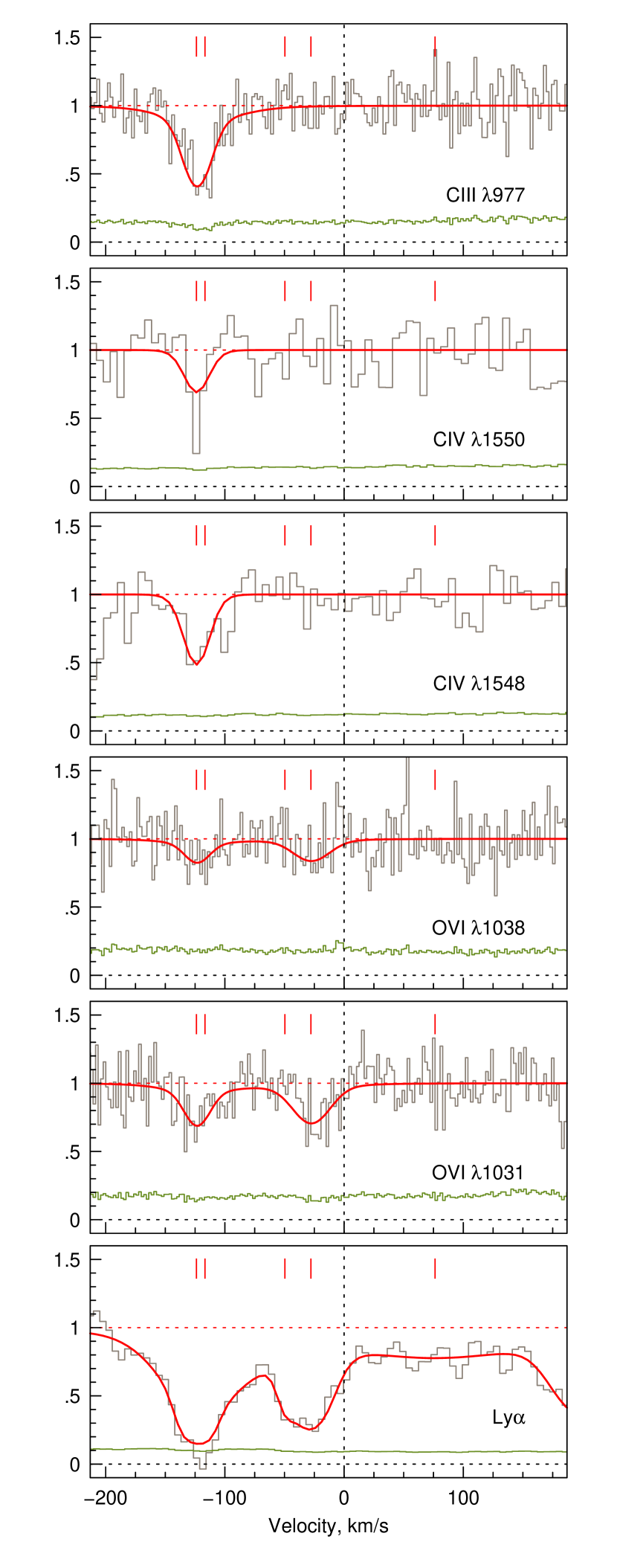
Figure 5.— Expanded region of the Voigt profile decomposition of the detected metal lines over the redshift window for clouds #7 through #11 of the Hi complex. The vertical dashed line is the redshift of galaxy G1.

In Paper I, we reported no detected metal absorption in Civ (STIS) and Ovi (FOS). However, we clearly detected Ovi absorption in the COS spectrum in the velocity range $-200\leq v\leq 0$ km s^-1 relative to $z_{\rm gal}=0.6719$. We also detected Ciii $\lambda 977$ absorption at $v\simeq-120$ km s^-1. We then re-examined the Civ absorption, and formally detected Civ $\lambda 1548$ aligned in velocity with the Ovi and Ciii absorption. The Civ $\lambda 1550$ absorption, which we had interpreted as noise in Paper I, is detected at the $3.5~{}\sigma$ level.

In Figure 5, the curves through the data are fitted VP components. For these fits, we modified MINFIT to hold the VP component redshifts (velocities) and Doppler $b$ parameters constant, allowing only the column densities to be $\chi^{2}$ minimized, and fitted the metal lines using the velocities and Doppler $b$ parameters from the VP fits to the Hi Lyman series lines. As with the Hi fits described above, the COS ISF (Dixon et al., 2010; Kriss, 2011) and the STIS ISF (Bostroem et al., 2010) appropriate for the spectrograph settings and the observed wavelength of each transition was determined via interpolation of the on-line tabulated data.

When a VP component column density was objectively determined to be insignificant, MINFIT returned an upper limit. Several tests for significance were conducted during the least-square fitting convergence; in short, for a column density to be deemed significant, the fitted VP value and its uncertainty had to be inconsistent with the upper limit on the column density (in that precise region of the spectrum and for that Doppler $b$ parameter), and the integrated apparent optical depth (Savage & Sembach, 1991) had to be consistent with the VP component and inconsistent with the the upper limit on the column density.

In Table 3, we list the metal-line absorption properties for all clouds. In MINFIT, the equivalent width limits are determined directly from the spectra using the methods of Schneider et al. (1993) and Churchill et al. (1999b), but modified for partially or fully resolved features (see Lawton et al., 2008). For each transition, we use the Doppler $b$ parameter from the VP fit to the Hi series convolved with the appropriate ISF to measure the upper limit on the equivalent width in each cloud. The uncertainty in the Doppler $b$ width is used to determine the $1~{}\sigma$ spread in this limit. The column density limits and the $1~{}\sigma$ spread in these are determined from the curve of growth.

5. Ionization Modeling

We employed our own photo+collisional ionization code (Churchill & Klimek, 2012), which is very similar to the code LINESPEC (Verner & Iakovlev, 1990). The code treats photoionization, Auger ionization, direct collisional ionization, excitation-autoionization, photo-recombination, high and low temperature dielectronic recombination, charge transfer ionization by H⁺, and charge transfer recombination by H⁰ and He⁰. Metals up to zinc can be incorporated, and all ionization stages for each elemental species are modeled. The code is appropriate for optically thin gas in which no ionization structure is present.

Table 3Selected Metal-Line Measurements

Cld#	$z_{cl}$	$v_{cl}$	$\log N({\hbox{{\rm Mg}\kern 1.00006pt{\sc ii}}})$	$\log N({\hbox{{\rm Si}\kern 1.00006pt{\sc iii}}})$	$\log N({\hbox{{\rm Si}\kern 1.00006pt{\sc iv}}})$	$\log N({\hbox{{\rm C}\kern 1.00006pt{\sc iii}}})$	$\log N({\hbox{{\rm C}\kern 1.00006pt{\sc iv}}})$	$\log N({\hbox{{\rm O}\kern 1.00006pt{\sc vi}}})$
		[km s-1]
1	0.668645	$-582.1$	$<\!\!11.70_{-0.30}^{+0.17}$	$<\!\!12.46_{-9.99}^{+0.16}$	$<\!\!13.07_{-9.99}^{+0.15}$	$<\!\!12.77_{-9.99}^{+0.16}$	$<\!\!13.26_{-9.99}^{+0.16}$	$<\!\!13.58_{-9.99}^{+0.16}$
2	0.668861	$-543.5$	$<\!\!11.53_{-0.18}^{+0.13}$	$<\!\!12.29_{-0.16}^{+0.11}$	$<\!\!12.92_{-0.13}^{+0.10}$	$<\!\!12.60_{-0.15}^{+0.11}$	$<\!\!13.12_{-0.16}^{+0.11}$	$<\!\!13.42_{-0.14}^{+0.11}$
3	0.669000	$-518.6$	$<\!\!11.50_{-0.25}^{+0.15}$	$<\!\!12.26_{-0.15}^{+0.13}$	$<\!\!12.90_{-9.99}^{+0.12}$	$<\!\!12.57_{-0.06}^{+0.14}$	$<\!\!13.09_{-0.12}^{+0.13}$	$<\!\!13.40_{-0.03}^{+0.13}$
4	0.669112	$-498.5$	$<\!\!11.21_{-0.07}^{+0.12}$	$<\!\!12.02_{-9.99}^{+0.08}$	$<\!\!12.79_{-9.99}^{+0.01}$	$<\!\!12.41_{-9.99}^{+0.05}$	$<\!\!12.87_{-9.99}^{+0.08}$	$<\!\!13.24_{-9.99}^{+0.01}$
5	0.669199	$-482.9$	$<\!\!11.25_{-0.11}^{+0.09}$	$<\!\!12.05_{-0.06}^{+0.06}$	$<\!\!12.78_{-9.99}^{+0.03}$	$<\!\!12.39_{-9.99}^{+0.04}$	$<\!\!12.90_{-9.99}^{+0.06}$	$<\!\!13.22_{-9.99}^{+0.04}$
6	0.669290	$-520.6$	$<\!\!11.54_{-0.20}^{+0.13}$	$<\!\!12.30_{-0.17}^{+0.12}$	$<\!\!12.93_{-0.14}^{+0.11}$	$<\!\!12.61_{-0.16}^{+0.12}$	$<\!\!13.13_{-0.17}^{+0.12}$	$<\!\!13.43_{-0.16}^{+0.12}$
7	0.671203	$-123.8$	$<\!\!11.48_{-0.06}^{+0.05}$	$<\!\!12.24_{-0.05}^{+0.04}$	$<\!\!12.89_{-0.04}^{+0.04}$	$13.24\pm 0.07$	$13.40\pm 0.08$	$13.49\pm 0.13$
8	0.671244	$-116.6$	$<\!\!11.76_{-0.08}^{+0.07}$	$<\!\!12.53_{-0.07}^{+0.06}$	$<\!\!13.12_{-0.07}^{+0.06}$	$12.42\pm 0.39$	$<\!\!13.33_{-0.07}^{+0.06}$	$12.89\pm 0.68$
9	0.671617	$-49.6$	$<\!\!11.33_{-0.18}^{+0.38}$	$<\!\!12.10_{-0.17}^{+0.31}$	$<\!\!12.81_{-0.16}^{+0.24}$	$<\!\!12.42_{-0.09}^{+0.31}$	$<\!\!12.95_{-0.15}^{+0.31}$	$<\!\!13.25_{-0.11}^{+0.30}$
10	0.671739	$-27.7$	$<\!\!11.58_{-0.10}^{+0.08}$	$<\!\!12.33_{-0.09}^{+0.07}$	$<\!\!12.96_{-0.08}^{+0.07}$	$<\!\!12.65_{-0.09}^{+0.07}$	$<\!\!13.16_{-0.09}^{+0.07}$	$13.62\pm 0.08$
11	0.672319	$+76.1$	$<\!\!11.91_{-0.14}^{+0.11}$	$<\!\!12.72_{-0.13}^{+0.10}$	$<\!\!13.25_{-0.13}^{+0.10}$	$<\!\!12.98_{-0.14}^{+0.10}$	$<\!\!13.47_{-0.14}^{+0.10}$	$<\!\!13.78_{-0.14}^{+0.10}$
12	0.672994	$+197.0$	$<\!\!11.65_{-0.11}^{+0.09}$	$<\!\!12.41_{-0.10}^{+0.08}$	$<\!\!13.03_{-0.09}^{+0.07}$	$<\!\!12.73_{-0.10}^{+0.08}$	$<\!\!13.23_{-0.10}^{+0.08}$	$<\!\!13.54_{-0.10}^{+0.08}$
13	0.673291	$+250.3$	$<\!\!11.66_{-0.10}^{+0.08}$	$<\!\!12.42_{-0.09}^{+0.07}$	$<\!\!13.04_{-0.08}^{+0.07}$	$<\!\!12.74_{-0.09}^{+0.07}$	$<\!\!13.24_{-0.09}^{+0.07}$	$<\!\!13.55_{-0.09}^{+0.07}$
14	0.673562	$+289.9$	$<\!\!11.46_{-0.18}^{+0.12}$	$<\!\!12.22_{-0.14}^{+0.10}$	$<\!\!12.87_{-0.10}^{+0.09}$	$<\!\!12.52_{-0.12}^{+0.11}$	$<\!\!13.05_{-0.14}^{+0.10}$	$<\!\!13.36_{-0.12}^{+0.11}$
15	0.673787	$+339.1$	$<\!\!11.73_{-0.09}^{+0.07}$	$<\!\!12.50_{-0.08}^{+0.07}$	$<\!\!13.09_{-0.08}^{+0.06}$	$<\!\!12.81_{-0.08}^{+0.07}$	$<\!\!13.30_{-0.08}^{+0.07}$	$<\!\!13.63_{-0.08}^{+0.07}$
16	0.674297	$+430.5$	$<\!\!11.65_{-0.09}^{+0.08}$	$<\!\!12.41_{-0.08}^{+0.07}$	$<\!\!13.03_{-0.08}^{+0.06}$	$<\!\!12.73_{-0.09}^{+0.07}$	$<\!\!13.22_{-0.08}^{+0.07}$	$<\!\!13.54_{-0.08}^{+0.07}$
17	0.674872	$+533.5$	$<\!\!11.71_{-0.06}^{+0.05}$	$<\!\!12.47_{-0.05}^{+0.05}$	$<\!\!13.08_{-0.05}^{+0.04}$	$<\!\!12.79_{-0.06}^{+0.05}$	$<\!\!13.28_{-0.05}^{+0.05}$	$<\!\!13.61_{-0.05}^{+0.05}$
18	0.675272	$+605.1$	$<\!\!11.71_{-0.03}^{+0.03}$	$<\!\!12.47_{-0.03}^{+0.02}$	$<\!\!13.07_{-0.02}^{+0.02}$	$<\!\!12.78_{-0.03}^{+0.02}$	$<\!\!13.28_{-0.03}^{+0.02}$	$<\!\!13.60_{-0.03}^{+0.02}$
19	0.675789	$+698.8$	$<\!\!11.67_{-0.03}^{+0.02}$	$<\!\!12.43_{-0.02}^{+0.02}$	$<\!\!13.05_{-0.02}^{+0.02}$	$<\!\!12.75_{-0.02}^{+0.02}$	$<\!\!13.25_{-0.02}^{+0.02}$	$<\!\!13.56_{-0.02}^{+0.02}$
20	0.676366	$+801.2$	$<\!\!11.60_{-0.09}^{+0.08}$	$<\!\!12.35_{-0.08}^{+0.07}$	$<\!\!12.99_{-0.07}^{+0.06}$	$<\!\!12.67_{-0.09}^{+0.07}$	$<\!\!13.18_{-0.08}^{+0.07}$	$<\!\!13.48_{-0.08}^{+0.07}$
21	0.676776	$+874.7$	$<\!\!11.70_{-0.02}^{+0.02}$	$<\!\!12.46_{-0.02}^{+0.02}$	$<\!\!13.07_{-0.02}^{+0.02}$	$<\!\!12.78_{-0.02}^{+0.02}$	$<\!\!13.27_{-0.02}^{+0.02}$	$<\!\!13.60_{-0.02}^{+0.02}$

The input cloud parameters are the hydrogen number density, $n_{\hbox{\tiny H}}$, equilibrium kinetic temperature, $T$, and the mass fraction of metals, $Z$. Solar abundance mass fractions are taken from Table 1.4 of Draine (2011), based upon Asplund et al. (2009), though the code has the option of modifying the relative abundances. A Haardt & Madau (2011) ionizing spectrum is used for the ultraviolet background (UVB). However, a stellar ionizing spectrum or a combined stellar plus UVB ionizing spectrum can be incorporated (see Churchill & Klimek, 2012, for details).

The code obtains an initial guess solution for the density of each ionic species based upon the assumption of adjacent ion stage ionization and recombination balance (i.e., neglecting Auger and charge transfer processes). Then, the rate matrix is solved using the code dqed.f, a Hanson/Krogh nonlinear least squares algorithm with linear constraints based on quadratic-tensor local model (Hanson, 1986). The outputs of the ionization code are the electron density, and the ionization and recombination rate coefficients, ionization fractions and the number densities for all ionic species.

Since the galaxy G1 is 58 kpc from the location where the gas is probed in absorption, and the stellar population is clearly dominated by red stars, we assume a UVB-only ionizing spectrum. We also assume a solar abundance pattern and include metals up to iron (however, we omitted lithium, beryllium, boron, fluorine, and the nobel gas elements for which many of the ionization and recombination rates are not well determined).

For a given cloud model, the resulting column density of ionic species X is obtained by

$$\log N({\rm X})=\log N({\hbox{{\rm H}\kern 1.00006pt{\sc i}}})-\log f_{\hbox{\tiny HI}}+\log n_{\hbox{\tiny X}}-\log\hbox{$n_{\hbox{\tiny H}}$}\,,$$ (1)

where $N({\hbox{{\rm H}\kern 1.00006pt{\sc i}}})$ is the Hi column density from the VP fit to the data, $n_{\hbox{\tiny H}}$ is the input hydrogen density of the cloud model, and where $f_{\hbox{\tiny HI}}$ is the ionization fraction of H⁰ and $n_{\hbox{\tiny X}}$ is the number density of ionic species X output by the code, respectively. Note that the metallicity of the model is implied. In practice, $n_{\hbox{\tiny X}}$ in a given model scales directly in proportion to $Z$. Thus, if the metallicity of the cloud model is $Z_{\rm m}$, for which the resulting density of species X is $n_{{\hbox{\tiny X}},{\rm m}}$, then $\log n_{\hbox{\tiny X}}=\log n_{{\hbox{\tiny X}},{\rm m}}+(\log Z-\log Z_{\rm m})$. For a given $n_{\hbox{\tiny H}}$, such scaling of the models is valid only if $f_{\hbox{\tiny HI}}$ is independent of metallicity, which holds for $\log Z/Z_{\odot}\leq-1$.

Comparing Eq. 1 to the measured values of $N({\rm X})$ from our VP fitting, we can constrain the metallicity and $n_{\hbox{\tiny H}}$ of each cloud. The range in these constrained quantities are based upon the $1~{}\sigma$ uncertainties in the measured column densities. Only three clouds have detected metal lines and therefore measured $N({\rm X})$. These clouds are #7, #8, and #10. We examine these clouds in the following subsections.

5.1. Clouds #7 and #8

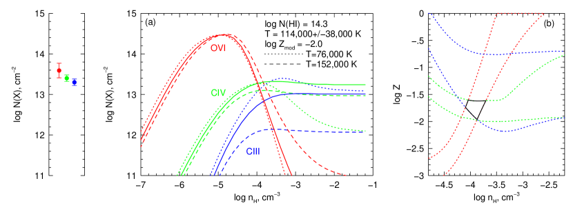
Figure 6.— ($a$) Ionization models of clouds #7+8 for a metal mass fraction of $\log Z/Z_{\odot}=-2.0$ with solar abundance ratios and temperature $T=114,000\pm 38,000$ K. The solid curves are the model column densities of Ovi (red), Civ (green), and Ciii (blue) and the dotted curves accounting for the uncertainties in the temperature. The measured values of $N({\hbox{{\rm O}\kern 1.00006pt{\sc vi}}})$, $N({\hbox{{\rm C}\kern 1.00006pt{\sc iv}}})$ and $N({\hbox{{\rm C}\kern 1.00006pt{\sc iii}}})$ are provided in the panel to the left. — ($b$) The $\log Z$–$\log n_{\hbox{\tiny H}}$ plane showing the constraints on the models from the measured data (same color scheme). Solid black curves provide the overlap regions.

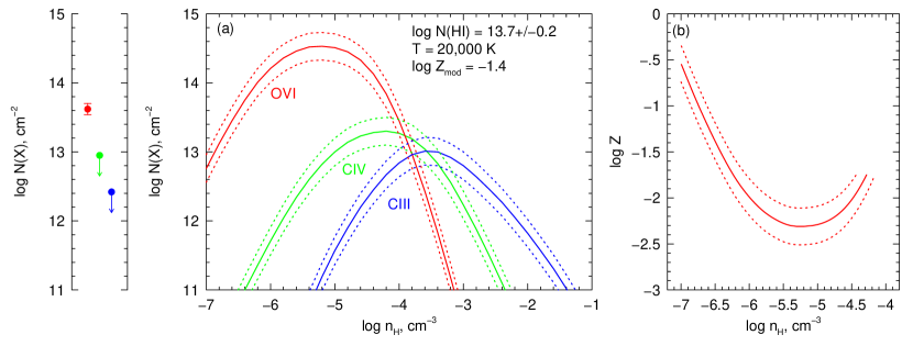
Figure 7.— ($a$) Ionization model of cloud #10 for a metal mass fraction of $\log Z/Z_{\odot}=-1.4$ with solar abundance ratios and temperature $T=20,000$ K. The solid curves and data points are as described in Figure 6, whereas the dotted curves account for a 0.2 dex error in $\log N({\hbox{{\rm H}\kern 1.00006pt{\sc i}}})$. — ($b$) The constrained range of the metal mass fraction on the $\log Z$–$\log n_{\hbox{\tiny H}}$ plane, accounting for the column density limits on the carbon ions.

Clouds #7 and #8 are located at $v\simeq-120$ km s^-1 with respect to the systemic velocity of G1 and are separated by $\Delta v=7$ km s^-1, which is on the order of half a single resolution element. The Hi profile is highly suggestive of a narrow plus a broad component combining to yield a deep core with a broad wing. The VP components reflect this profile shape, with cloud #7 providing the profile core, $\log N({\hbox{{\rm H}\kern 1.00006pt{\sc i}}})=14.1$ and $b({\hbox{{\rm H}\kern 1.00006pt{\sc i}}})=8$ km s^-1, and with cloud #8 providing the broadened wings, $\log N({\hbox{{\rm H}\kern 1.00006pt{\sc i}}})=13.7$ and $b({\hbox{{\rm H}\kern 1.00006pt{\sc i}}})=43$ km s^-1. The requirement for the broader cloud is significant at the 99% confidence level, even though some contribution to the blue portion of the broad wing is due to the extremely broad VP component (cloud #11) at $v=+76$ km s^-1.

At $v\simeq-120$ km s^-1, Ciii, Civ and Ovi are formally detected in the spectra. However, from the VP fitting, both clouds #7 and #8 have associated Ciii and Ovi, whereas only cloud #7 has associated Civ. Inspection of Figure 5 shows that the Civ absorption appears to be offset in velocity from the Ovi. However, the Civ is measured in the STIS spectrum, whereas the Ovi and Ciii are measured in the COS spectrum. Thus, the measured velocity offset relies heavily on the accuracy of the wavelength zero points between the two independent spectra.

Assuming thermal broadening, the implied temperature of cloud #7 is 8000 K, which is too cool to host strong Ovi and Civ absorption. The implied temperature of cloud #8 is $T=114,000\pm 38,000$ K, which is consistent with the temperature at which Civ absorption peaks for collisional ionization equilibrium. To analyze this absorption structure and constrain its hydrogen density and metallicity, we opted to assume a single phase of gas that is dominated by cloud #8 (however, in § 6.5 we also model these clouds as two distinct ionization phases). We added the Hi and metal column densities from clouds #7 and #8. For this exercise, we found that the column density limits for Mgii, Siiii, and Siiv did not contribute to constraining the gas properties.

In Figure 6, we illustrate our analysis of clouds #7+8. The ionization code was run for $-7\leq\log\hbox{$n_{\hbox{\tiny H}}$}\leq-1$ for $T=114,000$ K, and for $T=152,000$ and $T=76,000$, which brackets the $1~{}\sigma$ uncertainty in the temperature. In Figure 6$a$, we illustrate the model column densities for Ciii, Civ, and Ovi for $\log N({\hbox{{\rm H}\kern 1.00006pt{\sc i}}})=14.3$ and metallicity $\log Z/Z_{\odot}=-2.0$. In Figure 6$b$, we show the metallicity constraints as a function of $n_{\hbox{\tiny H}}$ for each metal ion, where the range in the constraints are based on the uncertainty in the temperature and the uncertainty in the Hi and metal ion column densities. The region of overlap indicates where the three ions provide consistent constraints on $n_{\hbox{\tiny H}}$ and $\log Z/Z_{\odot}$. Allowing for the uncertainties in the data, the gas is constrained to have $-4.2\leq\log\hbox{$n_{\hbox{\tiny H}}$}\leq-3.7$ and $-2.0\leq\log Z/Z_{\odot}\leq-1.6$ by all three metal ions. Note that metallicity is contrained primarily by $N({\hbox{{\rm C}\kern 1.00006pt{\sc iii}}})$, whereas hydrogen density is constrained primarily by $N({\hbox{{\rm O}\kern 1.00006pt{\sc vi}}})$.

5.2. Cloud #10

Cloud #10 is located at $v\simeq-30$ km s^-1 with respect to the systemic velocity of G1. It is optically thin in neutral hydrogen, with $\log N({\hbox{{\rm H}\kern 1.00006pt{\sc i}}})=13.7\pm 0.2$ and an implied temperature of $T=20,500\pm 8600$ K. The only detected metal line absorption is from Ovi, with $\log N({\hbox{{\rm O}\kern 1.00006pt{\sc vi}}})=13.6\pm 0.1$.

A high abundant the O⁺⁵ ion in a $T=20,000$ K cloud may be somewhat surprising. For $\hbox{$n_{\hbox{\tiny H}}$}\leq-3$ and $\log Z/Z_{\odot}=-2$, analysis of the rate coefficients output by the ionization code show that the balance of O⁺⁴, O⁺⁵, and O⁺⁶ is dominated by photoionization and recombination via charge exchange with H⁺, which dominates over free electron recombination by 2 orders of magnitude for O⁺⁵.

For cloud #10, the measured upper limit on Ciii is $\log N({\hbox{{\rm C}\kern 1.00006pt{\sc iii}}})\leq 12.7$ and on Civ is $\log N({\hbox{{\rm C}\kern 1.00006pt{\sc iv}}})\leq 13.2$. As with with our exercise for clouds #7+8, we found that the column density limits for Mgii, Siiii, and Siiv did not contribute to constraining the gas properties.

In Figure 7, we illustrate our analysis of cloud #10. The ionization code was run for $-7\leq\log\hbox{$n_{\hbox{\tiny H}}$}\leq-1$ for $T=20,000$ K. In Figure 7$a$, we show the column densities for Ciii, Civ, and Ovi for $\log N({\hbox{{\rm H}\kern 1.00006pt{\sc i}}})=13.7\pm 0.2$ and metallicity $\log Z/Z_{\odot}=-1.4$. The metallicity and hydrogen density constraints for cloud #10 are shown in Figure 7$b$.

If we account for the uncertainty in the implied temperature, we find that for $T=28,000$ K, the curves in Figure 7$b$ are unchanged for $\log\hbox{$n_{\hbox{\tiny H}}$}\geq-5.3$, and are shifted upward in the diagram by no more than 0.7 dex (higher $Z$ at a given $n_{\hbox{\tiny H}}$) for $\log\hbox{$n_{\hbox{\tiny H}}$}<-5.3$. As temperature is decreased, the curves shift to the upper right in the diagram such that at $T=12,000$ K, a minimum metallicity in the allowed range $-2.3\leq\log Z/Z_{\odot}\leq-1.8$ occurs at $\log\hbox{$n_{\hbox{\tiny H}}$}\geq-3.7$ instead of $-2.5\leq\log Z/Z_{\odot}\leq-2.0$ at $\log\hbox{$n_{\hbox{\tiny H}}$}=-5.3$. It seems less likely that Ovi absorption would be as strong as we detect in 12,000 degree gas.

5.3. Clouds with No Detected Metal Lines

The remainder of the Hi absorption complex is characterized by multiple components with gas temperatures in the range 20,000–90,000 K, though a hot, nearly million degree component is also present (cloud #11). For the clouds with no detected metals, the densities, ionization corrections, and therefore metallicities cannot be constrained without additional assumptions. In § 6.5, we assume hydrodynamic equilibrium and undertake an analysis of the clouds with only upper limits on the metal line column densities. Below, we motivate the assumption of hydrodynamic equilibrium as a reasonable scenario.

6. Inferred Physical Conditions of the Gas

6.1. Ionization Equilibrium and Cloud Stability

In general, ionization equilibrium is valid when the collisional ionization time scale, $\tau_{\rm coll}$, and the photoionization time scale, $\tau_{\rm ph}$, are shorter than the cooling time of the gas, $\tau_{\rm cool}$.

For a monatomic gas, the cooling time is the ratio of the energy per unit volume and the energy loss per unit volume per unit time, $\tau_{\rm cool}=Q/\dot{Q}=\,\hbox{\raisebox{2.15277pt}{\scriptsize 3}}\!/\!\hbox{\raisebox{-2.15277pt}{\scriptsize 2}}\,(n_{\rm e}+n_{\hbox{\tiny A}})\,kT/n_{\rm e}n_{\hbox{\tiny A}}\Lambda(T,Z)$, where $n_{\rm e}$ is the electron density, $n_{\hbox{\tiny A}}$ is the total density of all ions, and $\Lambda(T,Z)$ is the specific cooling function for metallicity $Z$. We obtain $n_{\rm e}$ and $n_{\hbox{\tiny A}}$ from our ionization code as a function of $n_{\hbox{\tiny H}}$ and $T$. Our cloud models are optically thin, such that $n_{\hbox{\tiny A}}\propto n_{\hbox{\tiny H}}$ and $n_{\rm e}\propto n_{\hbox{\tiny H}}$ at a given $T$, we thus find that the behavior of the cooling time follows $\tau_{\rm cool}\propto n_{\hbox{\tiny H}}^{-1}$ at fixed $T$.

We adopt the $Z=0$ specific cooling function of Sutherland & Dopita (1993) for a gas in collisional ionization equilibrium (also see Dopita & Sutherland, 2003). Since our models include photoionization, we corrected for photoionization heating (see Osterbrock & Ferland, 2006), which reduces the magnitude of $\dot{Q}$, and therefore increases the estimated cooling time. We found that photoionization heating from the UVB at $z=0.67$ is negligible for the density and temperatures ranges we explored.

Metals strongly contribute to the cooling rate, so the $Z=0$ curve provides an upper limit on the estimated cooling time under the assumption of ionization equilibrium. However, the effect is negligible for $\log Z/Z_{\odot}=-3$ and is a maximum difference of 0.4 dex at $\log T\simeq 5.3$ for $\log Z/Z_{\odot}=-2$ (see Sutherland & Dopita, 1993).

For a given ion, the collisional time scale is well approximated as $\tau_{\rm coll}\simeq 1/[n_{\rm e}(\alpha_{\rm rec}+\alpha_{\rm coll})]$, whereas the photoionization time scale is $\tau_{\rm ph}\simeq 1/R_{\rm ph}(J_{\nu})$, where $\alpha_{\rm rec}(T)$ and $\alpha_{\rm coll}(T)$ are the recombination and collisional ionization rate coefficients, and $R_{\rm ph}(J_{\nu})$ is the photoionization rate for the given ion, respectively. We obtain these quantities directly from our ionization code. Since $n_{\rm e}\propto n_{\hbox{\tiny H}}$ at a given $T$, we have $\tau_{\rm coll}\propto n_{\hbox{\tiny H}}^{-1}$ at fixed $T$. Thus, the ratio $\tau_{\rm cool}/\tau_{\rm coll}$ is effectively constant as a function of $n_{\hbox{\tiny H}}$ for fixed temperature. Note that for lower temperatures, $\alpha_{\rm coll}(T)$ vanishes so that $\tau_{\rm coll}$ becomes equal to the recombination time scale, $\tau_{\rm rec}\simeq 1/n_{\rm e}\alpha_{\rm rec}$.

Table 4Cloud Models of the Hi Complex

Cld#	$N({\hbox{{\rm H}\kern 1.00006pt{\sc i}}})$	$T$	$n_{\hbox{\tiny H}}$	$f_{\hbox{\tiny HI}}$	$\alpha_{\rm rec}$	$\alpha_{\rm coll}$	$\tau_{\rm cool}$	$\tau_{\rm coll}$	$\tau_{\rm dyn}$	$\tau_{\rm sc}$	$L$	$M_{g}$	$L_{J}$	$M_{J}$	Note
	[cm-2]	[K]	[cm-3]		[cm3 s-1]	[cm3 s-1]	[yr]	[yr]	[yr]	[yr]	[kpc]	[M⊙]	[kpc]	[M⊙]
7+8	14.30	5.06	$-5.0$	$-6.62$	$-13.21$	$-8.28$	9.40	5.70	10.01	11.71	4.43	15.84	2.73	10.72	JU
7+8	14.30	5.06	$-4.0$	$-5.69$	$-13.21$	$-8.28$	8.40	4.70	9.51	9.78	2.51	11.05	2.23	10.22	JU
7+8	14.30	5.06	$-3.0$	$-5.10$	$-13.21$	$-8.28$	7.40	3.70	9.01	8.19	0.91	7.27	1.73	9.72	EE
10	13.70	4.31	$-5.0$	$-6.02$	$-12.62$	-$11.36$	8.13	8.75	10.01	10.88	3.23	12.22	2.36	9.60	JU
10	13.70	4.31	$-4.0$	$-5.02$	$-12.62$	-$11.36$	7.13	7.76	9.51	8.88	1.23	7.22	1.86	9.10	EE
10	13.70	4.31	$-3.0$	$-4.03$	$-12.62$	-$11.36$	6.14	6.77	9.01	6.89	$-0.76$	2.25	1.36	8.60	EE
11	13.43	5.68	$-5.0$	$-7.22$	$-13.78$	$-7.57$	10.86	4.99	10.01	11.13	4.17	15.03	3.04	11.65	JU
11	13.43	5.68	$-4.0$	$-6.48$	$-13.78$	$-7.57$	9.86	3.99	9.51	9.39	2.43	10.81	2.54	11.15	EE
11	13.43	5.68	$-3.0$	$-6.23$	$-13.78$	$-7.57$	8.86	2.99	9.01	8.14	1.17	8.04	2.04	10.65	EE
15	13.68	4.95	$-5.0$	$-6.53$	$-13.12$	$-8.50$	9.06	5.92	10.01	11.05	3.72	13.69	2.68	10.56	JU
15	13.68	4.95	$-4.0$	$-5.58$	$-13.12$	$-8.50$	8.06	4.92	9.51	9.10	1.77	8.84	2.18	10.06	EE
15	13.68	4.95	$-3.0$	$-4.88$	$-13.12$	$-8.50$	7.06	3.93	9.01	7.40	0.07	4.73	1.68	9.56	EE
18	14.26	4.84	$-5.0$	$-6.43$	$-13.03$	$-8.78$	9.06	6.20	10.01	11.59	4.20	15.14	2.62	10.40	JU
18	14.26	4.84	$-4.0$	$-5.46$	$-13.03$	$-8.78$	8.06	5.20	9.51	9.62	2.23	10.23	2.12	9.90	JU
18	14.26	4.84	$-3.0$	$-4.66$	$-13.03$	$-8.78$	7.06	4.21	9.01	7.82	0.43	5.82	1.62	9.40	EE
20	13.10	4.41	$-5.0$	$-6.09$	$-12.69$	-$10.64$	8.41	8.05	10.01	10.30	2.70	10.63	2.41	9.75	JU
20	13.10	4.41	$-4.0$	$-5.09$	$-12.69$	-$10.64$	7.41	7.05	9.51	8.30	0.70	5.63	1.91	9.25	EE
20	13.10	4.41	$-3.0$	$-4.11$	$-12.69$	-$10.64$	6.41	6.07	9.01	6.32	$-1.28$	0.69	1.41	8.75	EE

6.2. Equilibrium Based On Hydrogen

In what follows, we briefly explore selected clouds using representative $n_{\hbox{\tiny H}}$ densities for the purpose of illustration. In Table 4, we present a summary of cloud models for the $n_{\hbox{\tiny H}}$ values $\log\hbox{$n_{\hbox{\tiny H}}$}=-5$, $-4$, and $-3$, where ion specific quantities apply for hydrogen. The hydrogen photoionization rate from the UVB at $z=0.67$ is $R_{\rm ph}=3.0\times 10^{-12}$ s^-1, yielding $\tau_{\rm ph}=1\times 10^{4}$ yr. As we shall see, the photoionization time is significantly shorter than the cooling times for all models; as such, only the longer collisional time scales constrain whether the clouds are in ionization equilibrium.

For clouds #7+8, at $T=114,000$ K, $\alpha_{\rm rec}=6.2\times 10^{-14}$ and $\alpha_{\rm coll}=5.3\times 10^{-9}$ cm³ s^-1, respectively. Assuming $\log\hbox{$n_{\hbox{\tiny H}}$}=-4$, we obtain $\tau_{\rm cool}\simeq 3\times 10^{8}$ yr and $\tau_{\rm coll}=5\times 10^{4}$ yr. With $\tau_{\rm cool}/\tau_{\rm coll}\simeq 5\times 10^{3}$, hydrogen is clearly in ionization equilibrium in clouds #7+8; the short photoionization and collisional ionization time scales relative to the recombination time scale are indicative of the highly ionized condition ($f_{\hbox{\tiny HI}}=2\times 10^{-6}$). The condition $\tau_{\rm ph}\lesssim\tau_{\rm coll}$ indicates photoionization marginally dominates over collisional ionization.

For cloud #10, at $T=20,000$ K, $\alpha_{\rm rec}=2.4\times 10^{-13}$ and $\alpha_{\rm coll}=4.3\times 10^{-12}$ cm³ s^-1. This cloud is constrained to have $\log\hbox{$n_{\hbox{\tiny H}}$}<-4$; assuming $\log\hbox{$n_{\hbox{\tiny H}}$}=-5$, we obtain $\tau_{\rm cool}\simeq 1\times 10^{8}$ yr and $\tau_{\rm coll}=6\times 10^{8}$ yr. For this assumed density, we find $\tau_{\rm cool}/\tau_{\rm coll}\simeq 0.2$, suggesting that ionization equilibrium may be marginal in cloud #10 for hydrogen (the gas temperature evolves on a similar time scale that the balance can be achieved). As listed in Table 4, the thermal time scale is shorter than the ionization time scale for the presented range of $n_{\hbox{\tiny H}}$.

For cloud #11, the hot, $\log T=5.68$ K, cloud, we have $\alpha_{\rm rec}=1.7\times 10^{-14}$ and $\alpha_{\rm coll}=2.7\times 10^{-8}$ cm³ s^-1. For $\log\hbox{$n_{\hbox{\tiny H}}$}=-4$ and $-5$, we obtain $\tau_{\rm cool}\simeq 7\times 10^{9-10}$ yr, and $\tau_{\rm coll}=1\times 10^{4-5}$ yr, where the longer times correspond to the lower density. Cloud #11 has $\tau_{\rm cool}/\tau_{\rm coll}\simeq 7\times 10^{5}$, indicating an ionization equilibrium condition. Note that if $\log\hbox{$n_{\hbox{\tiny H}}$}=-4$, we have $\tau_{\rm ph}\simeq\tau_{\rm coll}$, indicating that hydrogen ionization ($f_{\hbox{\tiny HI}}=3\times 10^{-7}$) is driven by both photo and collisional processes. If $\log\hbox{$n_{\hbox{\tiny H}}$}=-5$, then $f_{\hbox{\tiny HI}}=6\times 10^{-8}$, which is dominated by photoionization ($\tau_{\rm coll}/\tau_{\rm ph}=10$); the larger ratio due to the longer recombination time scale results in a higher ionization condition for this lower density.

With regard to the remaining clouds in the Hi complex with only limits on the metal line measurements, we selected clouds #15 [$\log N{(\hbox{{\rm H}\kern 1.00006pt{\sc i}}})=13.7,\log T=4.95$], #18 [$\log N{(\hbox{{\rm H}\kern 1.00006pt{\sc i}}})=14.3,\log T=4.84$], and #20 [$\log N{(\hbox{{\rm H}\kern 1.00006pt{\sc i}}})=13.1,\log T=4.41$] as representative. Of clouds with no detected metals, #15 has the highest temperature and an intermediate $N({\hbox{{\rm H}\kern 1.00006pt{\sc i}}})$ as compared to all clouds in the Hi complex. Cloud #20 has the lowest temperature and the smallest $N({\hbox{{\rm H}\kern 1.00006pt{\sc i}}})$, and cloud #18 has an intermediate temperature and the highest $N({\hbox{{\rm H}\kern 1.00006pt{\sc i}}})$. The models, for hydrogen, are given in Table 4. Note that $\tau_{\rm cool}>\tau_{\rm coll}$ for these representative clouds, indicating the validity of ionization equilibrium.

6.3. Equilibrium Based On O⁺⁵ and C⁺³

For strict ionization equilibrium to hold, the ionization time scales must be smaller than the cooling time for all ions. The same arguments invoked for hydrogen above apply to the metals. Consider the O⁺⁵ ion; the photoionization rate from the UVB at $z=0.67$ is $R_{\rm ph}=4.3\times 10^{-16}$ s^-1, which yields $\tau_{\rm ph}=7\times 10^{7}$ yr.

For clouds #7+8, at $T=114,000$ K, $\alpha_{\rm rec}$ and $\alpha_{\rm coll}$ are $3.7\times 10^{-12}$ and $3.8\times 10^{-16}$ cm³ s^-1, respectively. For $\log\hbox{$n_{\hbox{\tiny H}}$}=-4$, we obtain $\tau_{\rm coll}=\tau_{\rm rec}=7\times 10^{7}$ yr, where both scale in proportion to $n_{\hbox{\tiny H}}^{-1}$. We thus have $\tau_{\rm coll}=\tau_{\rm rec}\simeq 4\,\tau_{\rm cool}$ independent of $n_{\hbox{\tiny H}}$, indicating that the O⁺⁵ ion is marginally in ionization equilibrium. Similarly, we find $\tau_{\rm coll}\simeq 3\,\tau_{\rm cool}$ for C⁺³.

For cloud #10, at $T=20,000$ K, $\alpha_{\rm rec}=1.4\times 10^{-11}$ cm³ s^-1 and $\alpha_{\rm coll}$ is negligible, indicating that collisional processes have vanishing importance in the ionization balance of O⁺⁵. For $\log\hbox{$n_{\hbox{\tiny H}}$}=-5$, we obtain $\tau_{\rm coll}=\tau_{\rm rec}=2\times 10^{8}$ yr. For all densities, we have $\tau_{\rm cool}/\tau_{\rm coll}\simeq 0.8$. Similarly, for C⁺³, we find $\tau_{\rm cool}/\tau_{\rm coll}\simeq 0.3$. As with hydrogen, ionization equilibrium may be marginal for cloud #10 for O⁺⁵ and C⁺³.

For cloud #11, at $\log T=5.68$, we have $\alpha_{\rm rec}=1.2\times 10^{-12}$ and $\alpha_{\rm coll}=6.9\times 10^{-11}$ cm³ s^-1 for O⁺⁵. When $\log\hbox{$n_{\hbox{\tiny H}}$}=-4$, and $-5$, we obtain $\tau_{\rm coll}=4\times 10^{6-7}$ yr, where the longer times correspond to the lower density. We have $\tau_{\rm cool}/\tau_{\rm coll}\simeq 2000$ for which O⁺⁵ is predominantly in collisional equilibrium, i.e., $\tau_{\rm coll}/\tau_{\rm ph}\simeq 20$ if $\log\hbox{$n_{\hbox{\tiny H}}$}=-4$, and roughly equally balanced by photo and collisional equilibrium, i.e., $\tau_{\rm coll}\simeq\tau_{\rm ph}$ for $\log\hbox{$n_{\hbox{\tiny H}}$}=-5$. For C⁺³, we obtain $\tau_{\rm cool}/\tau_{\rm coll}\simeq 2\times 10^{4}$. Cloud #11 is clearly in ionization equilibrium.

For clouds #15, #18, and #20, we find $\tau_{\rm cool}/\tau_{\rm coll}\simeq 2$, $2$, and $1$, respectively for O⁺⁵. For C⁺³, we find $\tau_{\rm cool}/\tau_{\rm coll}\simeq 0.9$, $0.9$, and $0.4$, respectively. For these clouds, O⁺⁵ is marginally in ionization equilibrium, whereas C⁺³ is marginally not in equilibrium.

Note that the cooling times are 1–3 orders of magnitude shorter than the Hubble time, $\tau_{\hbox{\tiny H}}=1/H_{0}=1.4\times 10^{10}$ yr, except for cloud #11 for $\log\hbox{$n_{\hbox{\tiny H}}$}\leq-5$ (recall that the cooling time scales inversely with $n_{\hbox{\tiny H}}$ for fixed $T$). This would indicate that the cloud thermal conditions have evolved; however it is not possible to estimate the thermal histories of the clouds beyond speculating that they were hotter (and presumably less dense) at $z>0.67$. For $4\leq\log T\leq 4.7$ and for $5\leq\log T\leq 6$, the cooling time increases toward higher temperatures, so we can infer that the thermal evolution of clouds in these temperature was slower at epochs prior to $z=0.67$ assuming the cloud densities have not strongly evolved.

6.4. Dynamical Stability, Sizes, and Masses

In view of the inferred thermal evolution of the absorbing clouds, it is interesting to examine their dynamical stability. This can be achieved by comparing the cloud dynamical and sound crossing time scales. Additionally, it would be of interest to estimate the cloud sizes and masses.

To within a dimensionless factor of order unity, the dynamical time (see Lequeux, 2005, § 14.2.1), or free-fall time, of a cloud with total mass density $\rho=\rho_{g}/f_{g}=(A_{\hbox{\tiny H}}m_{\rm a}/x_{\hbox{\tiny H}}f_{g})\,\hbox{$n_{\hbox{\tiny H}}$}$, is $\tau_{\rm dyn}=1/\sqrt{G\rho}$, where $A_{\hbox{\tiny H}}$ is the atomic weight of hydrogen, $m_{\rm a}$ is the atomic mass unit, $x_{\hbox{\tiny H}}=0.72$ is the mass fraction of hydrogen and $f_{g}=\Omega_{b}/\Omega_{m}\simeq 0.16$ is the fraction of the baryonic mass in gas. Evaluating, we have $\tau_{\rm dyn}\simeq 3.2\times 10^{7}\hbox{$n_{\hbox{\tiny H}}$}^{-1/2}$ yr.

The sound crossing time is $\tau_{\rm sc}=L/c_{s}$, where $L$ is the physical length scale of the cloud and the sound speed is $c_{s}^{2}=\gamma P_{g}/\rho_{g}=\gamma kT/\mu m_{\rm a}$, where $P_{g}$ is the gas pressure, $\gamma=5/3$ for an ideal monatomic gas, and $\mu$ is the mean molecular weight. Our ionization models indicate that the clouds are highly ionized, so we assume $\mu=(2x_{\hbox{\tiny H}}+\,\hbox{\raisebox{2.15277pt}{\scriptsize 3}}\!/\!\hbox{\raisebox{-2.15277pt}{\scriptsize 4}}\,x_{\hbox{\tiny He}}+\,\hbox{\raisebox{2.15277pt}{\scriptsize 1}}\!/\!\hbox{\raisebox{-2.15277pt}{\scriptsize 2}}\,x_{\hbox{\tiny Z}})^{-1}\simeq 0.6$, appropriate for a fully ionized gas with $\log Z/Z_{\odot}\simeq-2$. We thus obtain, $\tau_{\rm sc}\simeq 6.4\times 10^{9}\,L\,T^{-1/2}$ yr, when $L$ is given in kpc.

The “absorption” length scale of the cloud can be estimated as the line of sight path length required to give rise to the measured $N({\hbox{{\rm H}\kern 1.00006pt{\sc i}}})$ for the inferred $n_{\hbox{\tiny H}}$ from the ionization models, $L=N({\hbox{{\rm H}\kern 1.00006pt{\sc i}}})/(f_{\hbox{\tiny HI}}\hbox{$n_{\hbox{\tiny H}}$})$. Assuming spherical geometry, the gas mass of the cloud is crudely estimated from $M_{g}=\rho_{g}L^{3}\simeq 3.4\times\!10^{7}\hbox{$n_{\hbox{\tiny H}}$}L^{3}$ M_⊙ when $L$ is given in kpc. A spherical geometry with unity volume filling factor is likely a very poor model, and one which will significantly overestimate the cloud mass. If the absorber geometry is cylindrical of length $L$ and radius $R$ with aspect ratio $\beta=2R/L$, then $M_{\rm cyl}/M_{\rm sph}\propto\beta^{2}$ if the line of sight probes parallel to $L$.

It is well established based on observational and theoretical grounds, that in general, Ly$\alpha$ forest clouds cannot be pressure confined (Rauch, 1998). Schaye (2001) convincingly argues that clouds which develop due to the gravitational influence of underlying dark matter density perturbations persist in a near hydrodynamic equilibrium state local to the region giving rise to the Ly$\alpha$ absorption. Effectively, this is equivalent to stating that the dynamical time is equal to the sound crossing time, $\tau_{\rm dyn}\simeq\tau_{\rm sc}$, consequently implying that the characteristic length of the absorbing region will be on the order of the local Jean’s length, $L_{J}$ (see Lequeux, 2005, § 14.1.2). Equating $\tau_{\rm dyn}$ and $\tau_{\rm sc}$, the Jean’s length is $L_{J}\simeq 5.0\times 10^{-3}\,(T/\hbox{$n_{\hbox{\tiny H}}$})^{1/2}$ kpc, from which the Jean’s gas mass can be estimated, $M_{J}=\rho_{g}L_{J}^{3}\simeq 4.3\,T^{3/2}\hbox{$n_{\hbox{\tiny H}}$}^{-1/2}$ M_⊙.

For $M_{g}>M_{J}$ the condition is $\tau_{\rm dyn}<\tau_{\rm sc}$; the cloud is Jean’s unstable to further gravitational contraction and will adjust on the dynamical time scale via fragmentation or due to shock processes. Conversely, for $M_{g}<M_{J}$ the condition is $\tau_{\rm sc}<\tau_{\rm dyn}$, and the cloud will adjust in the sound crossing time scale, either via evaporation or expansion (Schaye, 2001; Lequeux, 2005). The criterion assumes that the cloud is isolated, spherical, homogeneous, and exhibits no bulk motions.

The dynamical and sound crossing times, deduced cloud sizes and cloud gas masses are listed in Table 4 for cloud #7+8, #10, #11, and the representative clouds #15, #18, and #20 for $\log\hbox{$n_{\hbox{\tiny H}}$}=-3$, $-4$, and $-5$. As described above, cloud #7+8 is well constrained to have $\log\hbox{$n_{\hbox{\tiny H}}$}\simeq-4$, whereas cloud #10 and the remaining clouds with only limits on the metal line column densities are not well constrained.

For $\log\hbox{$n_{\hbox{\tiny H}}$}\leq-3$, $-4$, and $-5$, we obtain $\tau_{\rm dyn}\simeq 1\times 10^{9}$, $3\times 10^{9}$, and $1\times 10^{10}$ yr, respectively. Note that $\tau_{\rm dyn}\propto\hbox{$n_{\hbox{\tiny H}}$}^{-1}$, whereas $\tau_{\rm sc}\propto(f_{\hbox{\tiny HI}}\hbox{$n_{\hbox{\tiny H}}$})^{-1}$, and $\tau_{\rm cool}\propto\hbox{$n_{\hbox{\tiny H}}$}^{-1/2}$. The relative behavior of these times scales is such that a transition from $\tau_{\rm sc}<\tau_{\rm dyn}$ to $\tau_{\rm sc}>\tau_{\rm dyn}$ occurs as $n_{\hbox{\tiny H}}$ increases. This indicates that for larger $n_{\hbox{\tiny H}}$, the clouds have a propensity to be in the regime of Jean’s instability, whereas as for smaller $n_{\hbox{\tiny H}}$, the clouds become unstable to evaporation and expansion. The last column of Table 4 notes whether a cloud model is inferred to be Jean’s unstable (JU) or unstable to expansion and/or evaporation (EE). The behavior with $n_{\hbox{\tiny H}}$ suggests that between $-3\leq\log\hbox{$n_{\hbox{\tiny H}}$}\leq-5$ there is a density at which the clouds would classify as being in hydrodynamic equilibrium. This is also reflected in the behavior of the Jean’s lengths, $L_{J}$, which would be equivalent to the absorption length scales, $L$, when $\tau_{\rm dyn}=\tau_{\rm sc}$.

Note that the absorption scale lengths, $L$, and the cloud gas masses, $M_{g}$, become unphysically large as hydrogen density decreases. This would suggest that the clouds have $\log\hbox{$n_{\hbox{\tiny H}}$}>-5$, though we caution that the masses are probably overestimates due to the assumption of a spherical geometry. If more akin to cylindrical structures, viewed along the long axis, a factor of $\beta=0.1$ reduces the masses by two orders of magnitude. However, the absorption length scale along the line of sight is independent of geometry.

6.5. Hydrodynamic Equilibrium Conditions

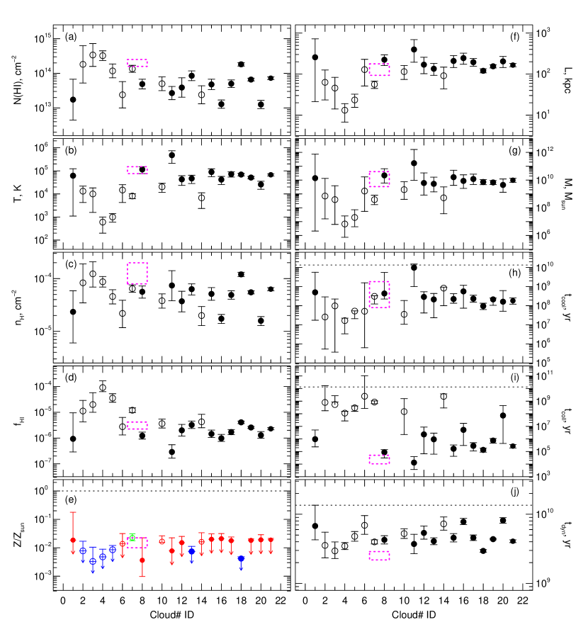
Figure 8.— The deduced cloud physical conditions under the assumption of hydrodynamic equilibrium. — ($a$) The measured $N({\hbox{{\rm H}\kern 1.00006pt{\sc i}}})$ from the VP fits. — ($b$) The measured temperature, based upon the VP Doppler $b$ parameter. — ($c$) The equilibrium $n_{\hbox{\tiny H}}$ computed from Eq. 2. — ($d$) The equilibrium hydrogen ionization fraction, $f_{\hbox{\tiny HI}}$, computed from Eq. 2. — ($e$) The metallicity, $Z/Z_{\odot}$, computed from Eq. 3; the points are colored coded based upon the ion that provides the most stringent constraints; red for O⁺⁵, green for C⁺³, and blue for C⁺². The dotted line is solar. — ($f$) The absorption scale length, $L=N({\hbox{{\rm H}\kern 1.00006pt{\sc i}}})/(f_{\hbox{\tiny HI}}\hbox{$n_{\hbox{\tiny H}}$})$. Note that this is equivalent to the Jean’s length, $L_{J}$, for the assumption of hydrodynamic equilibrium. — ($g$) The gas mass, $M_{g}$. Note that $M_{g}=M_{J}$, the Jean’s gas mass, for the assumption of hydrodynamic equilibrium. — ($h$) The cooling time, $\tau_{\rm cool}$; the dotted line is the Hubble time, $\tau_{\hbox{\tiny H}}=1/H_{0}$. — ($i$) The collisional time, $\tau_{\rm coll}$; the dotted line is $\tau_{\hbox{\tiny H}}$. — ($j$) The dynamical time, $t_{\rm dyn}$; the dotted line is $\tau_{\hbox{\tiny H}}$. Note that the sound crossing time, $\tau_{\rm sc}$ is equivalent to $\tau_{\rm dyn}$ for the assumption of hydrodynamic equilibrium. Open data points represent clouds that do not satisfy the criterion of hydrogen ionization equilibrium, where solid data points do satisfy the criterion. Dotted magenta boxes straddling clouds #7 and #8 represent the single-phase model presented in § 5.1 as illustrated in Figure 6.

In view of the arguments given by Schaye (2001) that Ly$\alpha$ clouds should be in the regime of hydrostatic equilibrium, and in view of the unphysically large cloud scale lengths we deduce in the regime of Jean’s instability, it is reasonable to explore the inferred cloud conditions under the assumption of hydrodynamic equilibrium. This assumption will yield an equilibrium value for $n_{\hbox{\tiny H}}$, from which the ionization conditions and metallicities can be constrained.

Equating the dynamical time and the sound crossing time, and invoking the absorption scale length, $L=N({\hbox{{\rm H}\kern 1.00006pt{\sc i}}})/(f_{\hbox{\tiny HI}}\hbox{$n_{\hbox{\tiny H}}$})$, we derive the condition of hydrodynamic equilibrium,

$$n_{\hbox{\tiny H}}\,x_{\hbox{\tiny H}}f_{g}\,\gamma kT\,[f_{\hbox{\tiny HI}}(n_{\hbox{\tiny H}},T)]^{2}=GA_{\hbox{\tiny H}}\mu m^{2}_{\rm a}\,[N({\hbox{{\rm H}\kern 1.00006pt{\sc i}}})]^{2}\,,$$ (2)

where $N({\hbox{{\rm H}\kern 1.00006pt{\sc i}}})$ and $T$ are measured from the VP fit models to the Ly$\alpha$ profiles, and $f_{\hbox{\tiny HI}}(\hbox{$n_{\hbox{\tiny H}}$},T)$ and $n_{\hbox{\tiny H}}$ are computed using ionization models of the clouds.

Since the hydrogen ionization fraction is a function of $n_{\hbox{\tiny H}}$, Eq. 2 is a transcendental equation and must therefore be solved numerically for the equilibrium hydrogen density for a cloud with temperature $T$. For each cloud, we interpolate a grid of ionization models with metallicity $\log Z_{\rm m}/Z_{\odot}=-2$ for $-6.0\leq\log\hbox{$n_{\hbox{\tiny H}}$}\leq-2.0$ in steps of $\Delta\log\hbox{$n_{\hbox{\tiny H}}$}=0.2$ and $2.6\leq\log T\leq 6.0$ in steps of $\Delta\log T=0.1$. We set $T$ equal to the measured cloud temperature (based upon the Doppler $b$ parameter from the VP fits), interpolate to obtain $f_{\hbox{\tiny HI}}(\hbox{$n_{\hbox{\tiny H}}$},T)$ as a function $n_{\hbox{\tiny H}}$ at that $T$, and iterate using Brent’s method to locate the $n_{\hbox{\tiny H}}$ that satisfies Eq. 2 to a tolerance $1\times 10^{-10}$. The method assumes that $f_{\hbox{\tiny HI}}(\hbox{$n_{\hbox{\tiny H}}$},T)$ is independent of metallicity (which we verified for $\log Z_{m}/Z_{\odot}\leq-1$).

For this exercise, we treat clouds #7 and #8 separately (i.e., as a multiphase structure as opposed to a single-phase cloud as done in § 5.1). We also omit cloud #9, which has a very uncertain Doppler $b$ parameter in that its temperature is consistent with $T=0$ K.

Once Eq. 2 is satisfied, the cloud absorption scale length, $L$, can be computed, from which the cloud gas mass can be estimated. Note that these quantities, while determined from the measured $N({\hbox{{\rm H}\kern 1.00006pt{\sc i}}})$ and $T$ as constrained by the ionization models, will be equivalent to the Jean’s length and Jean’s gas mass for the equilibrium $n_{\hbox{\tiny H}}$.

For each cloud, the uncertainty in the equilibrium $n_{\hbox{\tiny H}}$ and $f_{\hbox{\tiny HI}}$ are obtained by accounting for the measured uncertainties in both $N({\hbox{{\rm H}\kern 1.00006pt{\sc i}}})$ and $T$ from the VP fits. The uncertainties in $L$ account for the uncertainties in $N({\hbox{{\rm H}\kern 1.00006pt{\sc i}}})$, $n_{\hbox{\tiny H}}$, and $f_{\hbox{\tiny HI}}$. The uncertainties in $M_{g}$ account for the uncertainties in $\rho_{g}$ (due to $n_{\hbox{\tiny H}}$) and $L$.

Once the equilibrium values are determined, the cloud metallicities and their uncertainties can be estimated from the equilibrium ionization cloud model. Denoting this metallicity as $Z$ (in solar units), we have

$$\log Z=\log\left[\frac{N({\rm X})}{N({\hbox{{\rm H}\kern 1.00006pt{\sc i}}})}\right]_{\hbox{\tiny VP}}+\log\left[\frac{Z_{\rm m}f_{\hbox{\tiny HI}}\hbox{ $n_{\hbox{\tiny H}}$}}{n_{\hbox{\tiny X}}}\right]_{\rm eq}\,,$$ (3)

where $N({\hbox{{\rm H}\kern 1.00006pt{\sc i}}})$ is the measured neutral hydrogen column density obtained from the VP fit to the data, $N({\rm X})$ is the measured or upper limit on the column density species X from the VP modeling, and $n_{\hbox{\tiny X}}$ is the number density of species X from the ionization model for the equilibrium $f_{\hbox{\tiny HI}}$ and $n_{\hbox{\tiny H}}$ and the model metallicity $Z_{\rm m}$. That is, we scale the equilibrium ionization model with $Z_{\rm m}$ to obtain $Z$ and an estimate of its uncertainty.

In Figure 8, we present the deduced cloud properties under the assumption of hydrodynamic and ionization equilibrium. Solid data points satisfy the condition of hydrogen ionization equilibrium, whereas open data points do not. The measured $N({\hbox{{\rm H}\kern 1.00006pt{\sc i}}})$ and $T$ are shown in panels 8$a$ and 8$b$, respectively. The equilibrium $n_{\hbox{\tiny H}}$ and $f_{\hbox{\tiny HI}}$ are presented in panels 8$c$ and 8$d$, respectively. Note that, as suggested by the analysis presented in Table 4, the clouds have $-4.8\leq\log\hbox{$n_{\hbox{\tiny H}}$}\leq-3.8$ and $-6\leq\log f_{\hbox{\tiny HI}}\leq-4$.

The metallicities are plotted in Figure 8$e$. Except for clouds #7, #8, and #10, the metallicities are upper limits. For the assumption of single ionization phase clouds, each metal line provides a unique limit. The most stringent limits are presented, with the data point color coded by the ion that provides this best limit (red for O⁺⁵, green for C⁺³, and blue for C⁺²). In general, the upper limits are $\log Z/Z_{\odot}<-1.7$. The measured values for clouds #7, #8, and #10 are $\log Z/Z_{\odot}=-1.65^{+0.14}_{-0.10}$, $-2.44^{+0.79}_{-0.57}$, and $-1.78^{+0.20}_{-0.03}$, respectively.

The absorption scale length (which is equal to the Jean’s length under the assumption of hydrodynamic equilibrium), is shown in Figure 8$h$ for each cloud. The typical scale length is few hundred kpc, except for clouds #2, #3, #4, and #5, which have the lowest temperatures and thus relatively high densities and low ionization conditions. Recall, that the VP fits for clouds #1 through #6 should be viewed with caution. The gas masses, $M_{g}$, of the clouds (which equal the Jean’s gas masses under the assumption of hydrodynamic equilibrium) are presented in Figure 8$g$. Assuming spherical clouds, the gas masses are on the order of $10^{8}$-$10^{10}$ M_⊙, except for cloud #11, which has $M_{g}\simeq 10^{11}$ M_⊙. These mass estimates should be viewed as upper limits by as much as one to two orders of magnitude. Cloud #11 is the highest temperature cloud with the highest ionization condition. The larger mass is a result of the large scale length and the fact that the hydrogen density is relatively high, $\log\hbox{$n_{\hbox{\tiny H}}$}\simeq-4.1$.

The cooling time, $\tau_{\rm cool}$, is presented in panel 8$h$. Note that under the assumption of hydrodynamic equilibrium, the clouds have thermal stability in the order of 1–2 orders of magnitude shorter than the Hubble time. The collisional time, $\tau_{\rm coll}$, is presented in panel 8$i$. Except for clouds #10 and #14, the clouds are in ionization equilibrium. However, clouds #2 through #6 also may not be in ionization equilibrium; we again remind the reader that the VP fits to these latter clouds are to be viewed with caution. The dynamical time (which is equal to the sound crossing time under the assumption of hydrodynamic equilibrium), is presented in Figure 8$j$ for each cloud. In all cases, $\tau_{\rm dyn}$ and $\tau_{\rm sc}$ are a factor of a few less than the Hubble time, which is indicated by the dashed line.

The values obtained from this exercise are in remarkable agreement with those predicted from the simple scaling relations proposed by Schaye (2001) for the assumption of hydrodynamic equilibrium.

For comparison between the individual models of clouds #7 and #8 and the combined cloud #7+8 modeled in § 5.1, we indicate the results of the latter analysis as dashed boxes on Figure 8. For cloud #7+8, the measured column densities were summed, from which the density and metallicity were simultaneously constrained assuming a single ionization phase (see Figure 6). That analysis resulted in a slightly larger $n_{\hbox{\tiny H}}$ than the assumption of hydrodynamic equilibrium in the individual clouds, through the metallicities are consistent between analysis methods. The difference in $n_{\hbox{\tiny H}}$ is likely due to the adding of the column densities. We also compare the individual cloud equilibrium and the combined cloud $L$, $M_{g}$, $\tau_{\rm cool}$, and $\tau_{\rm dyn}$ $\tau_{\rm coll}$, shown as the dashed boxes on panels 8$f$–$j$. Note that cloud #7 has $\tau_{\rm coll}\gg\tau_{\rm ph}$, where $\tau_{\rm ph}=10^{4}$ yr, indicating that the hydrogen in this cooler cloud is photoionized. On the other hand, cloud #8 has $\tau_{\rm coll}\simeq\tau_{\rm ph}$ for both hydrogen and O⁺⁵, and thus has a substantial collisional ionization contribution.

Cloud #11 is of particular interest. This component is the hottest and most highly ionized, $f_{\hbox{\tiny HI}}\simeq 3\times 10^{-7}$, cloud in the complex, and is among the highest density, $\log n_{\hbox{\tiny H}}\simeq-4.1$, of the clouds. We find $\tau_{\rm coll}/\tau_{\rm ph}\simeq 1$ for hydrogen, and $\tau_{\rm coll}/\tau_{\rm ph}<100$ for O⁺⁵; thus hydrogen is equally photo and collisionally ionized, whereas O⁺⁵, though not detected, is predominantly collisionally ionized. It is plausible that this cloud (#11) is shock heated gas, as further suggested by the fact that the deduced cooling time ($\tau_{\rm cool}\simeq 10$ Gyr) is substantially longer than the deduced dynamical time ($\tau_{\rm dyn}\simeq 4$ Gyr). Crudely adopting the dynamical time as a proxy for the compression time (e.g., Birnboim & Dekel, 2003; Dekel & Birnboim, 2006), and considering the temperature and ionization conditions, we find that cloud #11 is the only component in the Hi complex that is suggestive of shocked gas.

6.6. Caveats

The analysis we have presented has employed many simplifying assumptions. The VP fitting method philosophy assumes that the gas structure comprises several spatially distinct isothermal clouds. In fact, it is very possible that the Hi complex is a quasi-continuous nonuniform structure with temperature and density variations having a range of bulk motions (and possibly at least one shock front, i.e., cloud #11). It is also plausible that such bulk motions can align in line of sight velocities creating caustics that emulate distinct clouds so that some VP components actually model a heterogeneous physical condition.

Furthermore, the analysis invoking the dynamical time, sound crossing time, and Jean’s mass and length is predicated on a homogeneous cloud. A cloud in thermodynamic equilibrium cannot simultaneously be homogeneous and isothermal, as we have assumed here.

In support of the assumption of hydrodynamic equilibrium, we note that Schaye (2001) argues that a spherical cloud with an isothermal density profile, i.e., $n_{\hbox{\tiny H}}(r)\propto r^{-2}$, has a well defined characteristic $n_{\hbox{\tiny H}}$ that is on the order of the maximum density probed by the line of sight. For the gas mass estimates, we have assumed spherical clouds, which is probably a very poor assumption. As such, the estimated gas masses should be considered upper limits.

Finally, the ionization modeling assumes photoionization and collisional ionization equilibrium, which we have shown to be a valid condition for the majority, but not all of the clouds. In addition, the metallicity estimates are based upon the assumption of single phase ionization conditions. If some of the plausible concerns expressed above with regard to heterogeneous physical conditions aligned in line of sight velocity hold, then multi-phase structure could be present that would affect the metallicity estimates. Overall, the assumption of ionization equilibrium in single phase gas is critical to all deduced quantities, especially the metallicities and the thermal equilibrium values presented in § 6.5.

7. Discussion

With a velocity extent of 1600 km s^-1, the Hi absorption complex at $z=0.672$ in the quasar Q1317+277 is a most intriguing gaseous structure. Absorption with velocity spreads on the order of $2000$ km s^-1 occur in approximately 10-15% of quasars (Weymann et al., 1991; Gibson et al., 2009). In almost all cases, extreme absorption of this nature is produced by material ejected from the quasar itself (i.e., broad absorption line quasars); however, the properties of the $z=0.672$ Hi complex studied here are not suggestive of absorption “associated” with or “intrinsic” to the quasar. For example, the Hi exhibits no evidence of partial covering, which is an adopted signature of associated gas (Barlow & Sargent, 1997; Ganguly et al., 1999). Furthermore, the kinematics of the metals absorption lines are kinematically similar to the velocity spreads observed in galaxy halos (Churchill & Vogt, 2001; Churchill et al., 2003). Thus, the Hi complex is likely inervening absorption. Early on, Bahcall & Salpeter (1965) suggested that the environments of galaxy clusters may give rise to extensive, intervening broad absorption line complexes, but few potential candidates have been identified.

In this section, we summarize and further examine the nature and environment of the $z=0.672$ Hi complex toward Q1317+277, compare it to other similar Hi complexes, and discuss the possible origin of the Q1317+277 Hi complex, such as hot-mode or cold-mode accretion, galactic winds, accreting filaments, intracluster gas, and/or the warm-hot phase of the intergalactic medium (WHIM).

7.1. The Nature of the $z=0.672$ Hi Complex

The Q1317+277 Hi complex at $z=0.672$ is characterized by a velocity spread of 1600 km s^-1 and 21 Ly$\alpha$ components with $12.9\leq\log N({\hbox{{\rm H}\kern 1.00006pt{\sc i}}})\leq 14.5$, as determined by Voigt profile fitting. Under the assumption that the components (clouds) are near hydrodynamic equilibrium, the temperatures, hydrogen number densities, and hydrogen ionization fractions primarily range between $10^{4}\leq T\leq 10^{5}$ K, $-3.9\leq\log n_{\hbox{\tiny H}}\leq-4.9$, and $-5.5\leq\log f_{\hbox{\tiny HI}}\leq-6.0$. The deduced cloud sizes are on the order of 200 kpc, and the cloud baryonic gas masses range between $10^{9}$–$10^{10}$ M_⊙. Because the gas masses scale as $n_{\hbox{\tiny H}}^{-2}f_{\hbox{\tiny HI}}^{-3}$, the large masses result from the low hydrogen number densities and the high ionization conditions of the clouds.

The metallicities are measured only for clouds #7, #8, and #10 and are $\log Z/Z_{\odot}=-1.7$, $-2.5$, and $-1.8$, respectively. Upper limits on the remaining clouds are $\log Z/Z_{\odot}<-2.4$ to $\log Z/Z_{\odot}<-1.7$. The limits on the cloud metallicities do not rule out enrichment at the level of the high redshift IGM (e.g., Cowie & Songaila, 1998; Simcoe et al., 2004). On the other hand, the low metallicities are 1–2 orders of magnitude below the $\log Z/Z_{\odot}\sim-0.6$ metallicities measured in $z=0.7$ X-ray clusters (Balestra et al., 2007; Maughan et al., 2008).

Further insight is gained by examination of the kinematic-ionization substructure. Near the velocity center of the complex, at $v\simeq 75$ km s^-1 with respect to the galaxy G1, is a hot $T=480,000$ K, collisionally ionized component (cloud #11), which is very likely shocked gas. The narrow velocity region just blueward of cloud #11 comprises four clouds, within which the only metal lines are detected. The general overall absorption morphology of these four components (clouds #7–10), is that of a double profile suggesting two absorbing structures contiguous in velocity space. Cloud #10, separated by $\simeq 50$ km s^-1 from cloud #11, has detected Ovi absorption, which is deduced to arise in cool $T=20$–30 K photoionized gas. Clouds #7 and #8, which have detected Ovi, Civ, and Ciii absorption, give rise to a single profile, which is best modeled with a narrow core (cloud #7, cool photoionized gas with $T\simeq 10,000$ K) and a broad component (cloud #8, hot collisionally ionized gas with $T=115,000$ K). The velocity centroids are separated by less than half of a single COS spectral resolution element of $\simeq 17$ km s^-1. In addition, cloud #9 appears to be a very narrow ($T<10,000$ K) blue wing of cloud #10 offset by $\simeq 20$ km s^-1 that overlaps with the red wing of cloud #8. These substructures may be suggestive of clouds moving through a hot, $T>10^{6}$ K, medium in which a conductive interfaces arises at the boundary between the cool, warm, and hot gas (e.g., Sembach et al., 2003).

Knowing the environment of the Hi complex and relationship to galaxies would be instrumental for a broader interpretation. The proximate galaxy is G1, which lies at $D=58$ kpc from the quasar line of sight and has a redshift very near the mean of the Hi complex. The virial mass of galaxy G1 is estimated to be within a factor of two of the virial mass of M87 ($M_{\rm vir}/M_{\odot}\simeq 10^{14}$, Strader et al., 2011), suggesting that galaxy G1 could be a central galaxy in a Virgo-like cluster. However, we find no clearly compelling evidence that G1 resides in a galaxy cluster or in a group with an X-ray emitting intracluster medium.

A search of the NASA Extragalactic Database (NED) and SIMBAD database yielded no reported X-ray measurements of Q1317+277. Within $4^{\prime}$ of Q1317+277, there are no sources in the ROSAT all-sky survey bright source catalog (Mickaelian et al., 2006; Voges et al., 1999). Of the five closest X-ray sources that are not identified either as a star or an AGN/quasar (which have known redshifts), one (1RXS J131954.5+253210) lies at $2^{\circ}$ from Q1317+277 (50 Mpc projected at $z=0.672$). The bright $R=15.1$ galaxy identified within 29 ″ of the X-rays would be 2 Mpc projected from this source at $z=0.672$. If the X-ray source is associated with this galaxy, it is likely that the galaxy and X-ray source reside at a redshift much lower than the Hi complex.

In the ROSAT HR1 band, a minimum of 0.04 cnts s^-1 is required for a source to be included in the ROSAT catalog. Applying this upper limit, and invoking the relationship (Mullis, 2001) between the count rate and the total flux in the band (accounting for the aperture correction), we estimate $L_{\hbox{\tiny X}}<2\times 10^{39}$ erg s^-1. This is four orders of magnitude below the expected X-ray luminosity of $2\times 10^{43}$ erg s^-1 for a cluster with a central galaxy of virial mass of G1, where we have employed the bolometric X-ray luminosity to virial mass scaling relation of Bryan & Norman (1998) and corrected for the X-ray band (see Mullis, 2001). The virial temperature of galaxy G1 is estimated to be on the order of $10^{7}$ K, which yields a coronal temperature of $kT\simeq 0.8$ keV. According to the compilation of Crain et al. (2011), our upper limit on $L_{\hbox{\tiny X}}$ is not inconsistent with the observed X-ray luminosities of early-type galaxies with similar $kT$.

We have successfully measured spectroscopic redshifts for only galaxies G1 and G2. As such, we cannot directly deduce the presence of a cluster at $z=0.672$, nor estimate the velocity dispersion of the galaxies that may reside at this redshift. Based upon the photometric properties examined in the imaging date, it is difficult to definitively rule out or favor the presence of a cluster at $z=0.67$. However, the upper limits on the X-ray flux within 50 Mpc projected from Q1317+277 and the low metallicity of the Hi complex, 1-2 dex below intracluster gas measurements (Balestra et al., 2007; Maughan et al., 2008), do not favor a large cluster nor a hot intracluster medium.

Such considerations leave open the possibility that the Hi complex may be a phenomenon closely linked to a massive old elliptical galaxy that is not in an overdense environment. Taken together at face value, the data and the results of our analysis suggest a low metallicity structure, possibly a filament or the remnants of a disrupted filament. There remains the question of the possible connection to the smaller galaxy G3, which unfortunately does not have a measured or estimated redshift.

7.2. Review of Comparable Hi Complexes

Given the dramatic velocity spread and kinematics of the Hi complex toward Q1317+277, and given its proximity to galaxy G1 (and possibly G3), it is of interest to investigate how rare/common are such absorbing complexes, what their observed relationships are with respect to galaxies, and what interpretations have been adopted in view of the role of gas in the evolution of individual and group galaxies. Such insights may help identify the Q1317+277 Hi complex in a broader context.

One example is the $z\simeq 2$ Civ absorber complex toward the “Tololo Pair” (Tol 1037–27, $z_{\rm em}=2.18$, and Tol 1038–27, $z_{\rm em}=2.33$), which may be produced by intracluster gas (Jakobsen et al., 1986). The Civ doublets, later observed in two additional quasars in proximity on the sky, exhibit multiple discrete components with velocity widths ranging between 50–1000 km s^-1 and may extend some 18 Mpc (Dinshaw & Impey, 1996).

Another possible intracluster absorption complex, at $z=0.695$ toward the $z_{em}=1.05$ quasar PG 2302+029 (Jannuzi et al., 1996), exhibits broad ($\Delta v=3000$ km s^-1) high ionization Civ, Nv, and Ovi doublets. In the FOS spectrum (velocity resolution $\Delta v=230$ km s^-1), the Ly$\alpha$ absorption is segregated into multiple individual components each with $\Delta v<250$ km s^-1 distributed across the full velocity range of the metals. Near the central velocity, narrow Civ, Nv, and Ovi are present in one Ly$\alpha$ component. No low ionization species are present. Jannuzi et al. (1996) suggest three possible interpretations: (1) material ejected from the quasar at extreme ejection velocity, (2) material associated with galaxies or the intracluster medium of a cluster or supercluster of galaxies, and (3) remnant material from supernovae in a galaxy. Unfortunately, their observations did not provide data capable of distinguishing between these scenarios.

Toward the $z_{\rm em}=0.297$ quasar H1821+643, Tripp et al. (2001) reported an Hi complex at $z=0.1212$ comprising five Ly$\alpha$ components distributed over a velocity interval of $\sim 700$ km s^-1 in high resolution STIS and FUSE spectra. The $\log N({\hbox{{\rm H}\kern 1.00006pt{\sc i}}})$ column densities range from 12.7–13.8. Absorption from Ovi is present in a single broad wing of the central component, for which collisional ionization is favored with $T=10^{5.3-5.6}$ K and $-1.8\leq\hbox{[O/H]}\leq-0.6$. Seven galaxies in the velocity range of the absorption are present at impact parameters ranging from 140–2400 kpc, with the 140 kpc galaxy aligned in redshift with the Ovi absorption. Tripp et al. (2001) favor the scenario in which the Hi complex is intragroup gas or an unvirialized filamentary structure.

Using GHRS, STIS and FUSE spectra of the $z_{\rm em}=0.116$ BL Lac object PKS 2155–304, Shull et al. (1998) and Shull et al. (2003) analyzed an Hi complex with 14 Ly$\alpha$ components centered at $z=0.056$ spread over a velocity interval of 2270 km s^-1. They estimate the Hi column densities have the range $14.5\leq\log N({\hbox{{\rm H}\kern 1.00006pt{\sc i}}})\leq 15.0$ with $\log Z/Z_{\odot}<-2.5$ and cloud depths less than 400 kpc. Five Hi emitting galaxies are found in the range $0.056\leq z\leq 0.058$ with impact parameters 400–790 kpc. The two strongest Ly$\alpha$ blends have detectable Ovi and possible Oviii absorption measured in a Chandra spectrum. If the gas is the warm-hot ionized medium (WHIM) then the density is constrained to $\log n_{\hbox{\tiny H}}\simeq-4$. Shull et al. (2003) favor a scenario in which the Ovi arises in “nearside” and “backside” shocked infall into the potential well of the galaxy group.

In high resolution STIS and FUSE spectra of the $z_{\rm em}=0.370$ quasar HS 0624+6907, Aracil et al. (2006a) report a cluster of 13 Ly$\alpha$ lines at $z=0.0635$ with a velocity spread of 1000 km s^-1. The Hi column densities range between $12.6\leq\log N({\hbox{{\rm H}\kern 1.00006pt{\sc i}}})\leq 15.3$. Only in the central component, with total $\log N({\hbox{{\rm H}\kern 1.00006pt{\sc i}}})=15.4$, are metal lines detected (Siiii, Siiv, and Civ, but no Ovi) from which the gas is deduced to be photoionized with metallicity $\log Z/Z_{\odot}=-0.05$, very near to solar enrichment, with $\log n_{\hbox{\tiny H}}=-3.9$. The gas temperatures are deduced to be $T<10^{5}$ K. The estimated baryonic mass of this component is $\sim 10^{5}$ M_⊙ with an absorption length scale of 3–5 kpc. They report 10 galaxies within 135–1370 kpc in the range $0.062\leq z\leq 0.067$, but this group is not consistent with elliptical-rich groups. On account of the high metallicity and cool temperatures, Aracil et al. (2006a) favor the interpretation that this Hi complex is tidally stripped material from one of the nearby galaxies.

The Hi complexes toward H1821+643, PKS 2155–304, and HS 0624+6907 have both similarities and differences with the Hi complex toward Q1317+277. However, the Q1317+277 Hi complex bares little resemblance to the metal-rich complexes observed toward PG 2303+029 and toward the Tol 1037–27 and Tol 1038–27 pair. These latter two complexes may be examples of metal enriched intracluster gas.

The broad Hi component in the complex toward H1821+643 exhibits Ovi that is likely to be predominantly collisionally ionized with a relatively high metallicity. Similarly, cloud #8 in the Q1317+277 Hi complex appears to be a $T>10^{5}$ K, collisionally ionized Ovi absorber, but accompanied by Civ and Ciii absorption. On the other hand, the hottest, broad component in the Q1317+277 Hi complex has no detected Ovi and has upper limits on metallicity indicating that it is metal poor in comparison. The H1821+643 Ovi absorber is at a substantially larger impact parameter to the nearest galaxy, which resides in a group that clearly has no massive elliptical galaxy, whereas the Q1317+277 Hi complex quite is very close in projected to the massive elliptical galaxy G1.

The Hi column density for the low metallicity Ovi absorber in the complex absorption toward PKS 2155–304 is 1–2 orders of magnitude greater than the $N({\hbox{{\rm H}\kern 1.00006pt{\sc i}}})$ of the components in the Q1317+277 Hi complex. However, the clouds have similar $n_{\hbox{\tiny H}}$. In both complexes, the Ovi resides to the wings of largest Ly$\alpha$ components. Shull et al. (2003) interpret this as a shock interface, and this interpretation may apply in the case of the Q1317+277 Hi complex. However, as with the H1821+643 Ovi absorber, the environment of the PKS 2155–304 Hi complex resides within a moderate group of galaxies having no massive elliptical galaxy.

Of the three examples, the Hi complex toward HS 0624+6907 has an Hi absorption profile morphology most similar to that of the Q1317+277 Hi complex. The cool photoionized cloud with Civ, Siiv, and Siiii absorption compares to the cool photoionized Ovi absorbing cloud # 10 in the Q1317+277 Hi complex, but cloud # 10 has no Siiv or Civ absorption. Though the clouds have similar $n_{\hbox{\tiny H}}$, cloud #10 has lower $N({\hbox{{\rm H}\kern 1.00006pt{\sc i}}})$, higher ionization conditions, and a much lower metallicity as compared to the nearly solar metallicity cloud in the HS 0624+6907 complex. Because of the low ionization deduced for the latter cloud, the mass is $\sim 4$ orders of magnitude smaller than the mass deduced for cloud # 10. Again, the galaxy environment of the HS 0624+6907 Hi complex contains no massive elliptical galaxy.

Overall, two unique features to the Q1317+277 Hi complex are that it is at substantially higher redshift ($z=0.672$) compared to the other reported Hi complexes ($z=0.056$, $0.064$ and $0.121$) and that it is in close projected proximity to a region dominated by massive, metal-rich elliptical with an old stellar population.

7.3. Interpreting the $z=0.672$ Hi Complex

Summarizing the gas properties of the Q1317+277 Hi complex, we find (1) a hot, photo and collisionally ionized component that is consistent with shocked gas, (2) a cool component with photoionized Ovi absorption, and (3) a cool component plausibly layered within a warm component that is both photo and collisionally ionized and exhibits Ovi, Civ and Ciii absorption, (4) several additional warm Hi components spread over 1600 km s^-1 in the rest-frame of $z=0.672$, and (5) measurements of and limits on metal-enrichment between $-2.5\leq\log Z/Z_{\odot}\leq-1.7$.

If the rest-frame velocity spread of the Hi complex is due to the local Hubble flow, then the line-of-sight proper length of the structure would be $D_{\hbox{\tiny HF}}=\Delta v/H_{0}E(z)$, where $\Delta v=1600$ km s^-1 and $E^{2}(z)=\Omega_{m}(1+z)^{3}+\Omega_{\Lambda}$. At $z=0.67$, we estimate $D_{\hbox{\tiny HF}}\sim 15$ Mpc. Based upon the ionization modeling, the deduced physical sizes of the the Hi complex are not consistent with a single structure of this extent. If the velocities of the Hi absorbers are due to Hubble flow, then the complex must comprise absorbers that are spatially segregated; there are five main absorption features apparent in the Ly$\alpha$ profile, which would imply an average separation of 3 Mpc and that we have by chanced probed several isolated absorption systems. Considering the similarities of the properties of the Hi complexes toward H1821+643, PKS 2155–304, and HS 0624+6907, and that they are clearly connected with galaxies on scales of 0.1–1 Mpc, we do not favor the interpretation that the Q1317+277 Hi complex is multiple individual absorbers tracing a 15 Mpc Hubble flow.

Is it reasonable that the individual peaks in the Hi column density are a result of having fragmented from a single structure? If this structure were Jean’s unstable, i.e., $\tau_{\rm dyn}\ll\tau_{\rm sc}$, then fragmentation and/or shock disruption into the observed components would be plausible.

Crudely modeling this hypothetical single structure as having the $N({\hbox{{\rm H}\kern 1.00006pt{\sc i}}})$ weighted mean temperature of the components, $\left<\log T\right>=4.65$ (prior to fragmentation or shock disruption, where the latter could subsequently heat the shocked components), and assuming that the length of its long axis is the sum of the Jean’s lengths for each of the components, we find that $\tau_{\rm dyn}\simeq\,\hbox{\raisebox{2.15277pt}{\scriptsize 1}}\!/\!\hbox{\raisebox{-2.15277pt}{\scriptsize 20}}\,\tau_{\rm sc}$ independent of the assumed mean hydrogen density, $\bar{n}_{\hbox{\tiny H}}$, where $\tau_{\rm dyn}\simeq 3\times 10^{9}\,(\bar{n}_{\hbox{\tiny H}}/10^{-4})^{1/2}$ and $\tau_{\rm sc}\simeq 6\times 10^{10}\,(\bar{n}_{\hbox{\tiny H}}/10^{-4})^{1/2}$ yr. The model is consistent with the plausibility that the multiple component structure of the Hi absorption complex could very well have resulted from the fragmentation of a quasi-coherent single gaseous structure.

Our simple model yields a total Jean’s length of $L_{J}\simeq 2\,(\bar{n}_{\hbox{\tiny H}}/10^{-4})^{1/2}$ Mpc and a total Jean’s mass of $M_{J}\simeq 2\times 10^{11}\,(\bar{n}_{\hbox{\tiny H}}/10^{-4})^{1/2}$ Mpc, where the total mass is simply the sum of the Jean’s masses for the individual components. The implied aspect ratio $\beta=2R/L$ for a cylindrical structure is $\beta\simeq(M_{J}/\bar{\rho}_{g}L_{J}^{3})\simeq 0.1$. If $\log\bar{n}_{\hbox{\tiny H}}=-4$, then the Hi complex could be crudely envisioned as a $10^{11}$ M_⊙ mass cylindrical filament 2 Mpc long with a 200 kpc diameter. These values would scale as $(\bar{n}_{\hbox{\tiny H}})^{1/2}$.

Summarizing the luminous environment of the Hi complex, we find (1) a massive, red, high-metallicity, elliptical galaxy (G1) with an old stellar population ($\sim 6$ Gyr) residing at $D=58$ kpc and aligned in velocity between the shocked Hi component and the metal-enriched Hi components, near the Hi profile velocity centroid, and (2) the upper limits on the X-ray luminosity consistent with the measured range for ellipticals with $kT\simeq 0.8$ keV and well below expected values for clusters dominated by massive ellipticals.

In addition to the X-ray data not supporting the idea that galaxy G1 resides in a large cluster, the metallicity of the Hi absorbing gas is constrained to be 1-2 orders of magnitude below the average enrichment of clusters at $z=0.7$ (Balestra et al., 2007; Maughan et al., 2008). The observations of Brinchmann & Ellis (2000) and van der Wel et al. (2005) indicate that old, massive, metal-rich late-type galaxies were present in the field as early as $z=2$–$3$. The stellar population models for galaxy G1 suggest a formation epoch at $z\simeq 4$. It may be that galaxy G1 is not a dominant elliptical galaxy of a large group, but may be a galaxy in the field that formed at high redshift.

In addition to the aforementioned supporting observations, a massive, red, metal-rich elliptical far from a cluster environment is theoretically plausible. The cosmological simulations of Gabor & Davé (2012), which treat accretion and feedback processes, yield a substantial fraction of red, high mass galaxies independent of overdensity. Johansson et al. (2012) demonstrate that massive early-type galaxies are built in two phases. The first is an initial growth via in situ star formation fed by cold accretion ($z>3$) that is later quenched via virial shocking (e.g., Birnboim & Dekel, 2003; Kereš et al., 2005; Dekel & Birnboim, 2006; Kereš et al., 2009; van de Voort et al., 2011; van de Voort & Schaye, 2011). The second phase is accretion of stellar material ($z\sim 1.5$–$0.5$), called “dry minor mergers” due to the fact that their gas is heated and stripped by shock heating in the hot virial halo of the massive galaxy (e.g., Khochfar & Silk, 2009; Hopkins et al., 2010). These general results are also found by Naab et al. (2007, 2009).

With a mass of $\log M_{\rm vir}/M_{\odot}>13$, galaxy G1 is well above the “critical mass” where the cooling time of the gas is much longer than the dynamical time, such that an accretion shock is established near the virial radius (e.g., Birnboim & Dekel, 2003; Dekel & Birnboim, 2006; Kereš et al., 2009; van de Voort & Schaye, 2011). The rate at which the cooling time increases with decreasing redshift [$\tau_{\rm cool}\propto 1/\rho\propto(1+z)^{-3}$] is more rapid than the increase in the dynamical time with decreasing redshift, [$\tau_{\rm dyn}\propto 1/\sqrt{\rho}\propto(1+z)^{-3/2}$]. Thus, it is generally found in simulations that, at high redshifts, cold streams can often penetrate the hot halos and accrete onto the galaxies, whereas at intermediate to low redshifts, the longer cooling time results in the heating and shocking of the cold filaments, which then accrete into the halo but not onto the galaxy (Kereš et al., 2005; Dekel & Birnboim, 2006; Faucher-Giguère et al., 2011; van de Voort et al., 2011). Galaxy G1 may have experienced the process in which it formed stars early during its initial accretion, perhaps even experiencing cold accretion from the filament that we are observing, and then at later times the accretion penetrated no further than into the halo, resulting in a high mass, metal-rich, early-type galaxy with quenched star formation.

Given such a scenario, the Hi complex could be interpreted as a filamentary structure with IGM chemical enrichment levels that is undergoing shock disruption near the viral radius of galaxy G1. The hot cloud (#11) exhibits the signature of the shocked portion of the filament, and the multiphase absorbers (clouds #8-10) exhibit the signature of a conductive interface. Galaxy G1 is probed by the quasar sight line impact parameter at $D/R_{\rm vir}\simeq 0.1$. Simulations indicate that “cold” filaments (i.e., those that have not been heated above $\log T=5.5$) penetrate no deeper than $R\simeq 0.5R_{\rm vir}$ at intermediate redshifts (Kereš et al., 2009; van de Voort et al., 2011), suggesting that the sight line is intercepting the filament in the outer part of the virialized halo.

A cartoon model of this interpretation is illustrated in Figure 9. The cartoon is consistent with simulation results and is guided by inspection of Figure 7 (top panel, for a $z=2$, $M_{\rm vir}=10^{12}$ M_⊙ galaxy) from van de Voort et al. (2011) and the “cold only” panel of Figure 6 for a $z=1$ , $M_{\rm vir}=10^{13}$ M_⊙ galaxy from Kereš et al. (2009).

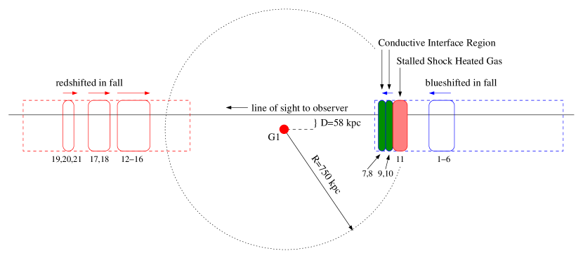
Figure 9.— A cartoon model illustrating the interpretation of the Hi absorbing complex as an accreting filament onto the galaxy G1. The positive velocity material would require that it is infalling from the oberver’s side of the galaxy, whereas the negative velocity material would be infalling opposite the observer’s side of the galaxy. The plausible relative physical locations of the absorbing clouds, labeled by their VP component numbers (see Table 2), are shown. The conductive interface (clouds #7-10) continue their infall after being stalled in a shock front, which is presently coincident with cloud #11 (see text). The model is adapted from simulation results (e.g., see the “cold only” panel of Figure 6 in Kereš et al., 2009).

Presumably, any components of the filament that have not yet been shocked will be shock heated and their cooling time will increase to be on the order of the Hubble time (as is deduced for cloud #11). Those components that may reside within the shock radius will likely not survive past $R\simeq 0.5R_{\rm vir}$ and be assimilated into the hot halo. This would imply that, ultimately, the filament will accrete into the halo, be heated to the halo temperature, and never accrete onto the galaxy itself. Galaxy G1 has likely not had new gas to fuel star formation for several Gigayears and will likely not acquire new gas via accretion as it evolves. Apart from the possibility of dry minor mergers (Khochfar & Silk, 2009; Hopkins et al., 2010; Johansson et al., 2012) building the stellar mass of galaxy G1, it is likely that the galaxy has experienced secular stellar evolution since $z=4$.

If galaxy G3 is at $z\simeq 0.67$, one might ask if the filament is associated with this lower mass $\log M_{\rm vir}/M_{\odot}\simeq 11.9$ galaxy. With the data in hand, it is nearly impossible to claim any relationship between galaxy G3, the Hi complex, and galaxy G1. However, a virial shock is not predicted for lower mass galaxies, which have cooling times shorter than their dynamical times. As such, it would be expected that a filament accreting onto galaxy G3 would not show the signature of shocked gas with conductive interfaces as seen in the Hi complex. It could be speculated that galaxy G3 is embedded in the filament, perhaps contributing to some in situ metal enrichment, and might eventually be a dry minor merger (2% mass ratio) with galaxy G1.

This scenario for the evolution of galaxy G1 is in stark contrast to the evolution of spiral galaxy G2, which is observed to have on-going star formation at $z=0.661$, likely due to on-going multiphase accretion that is feeding the galaxy (Kacprzak et al., 2012). To the limit of $\log N({\hbox{{\rm H}\kern 1.00006pt{\sc i}}})\simeq 12.4$, there is no indication in the COS spectrum of absorbing gas that bridges these two galaxies, which are separated by $\Delta v=1960$ km s^-1 (in the frame of the galaxies).

The scenario of a shock heated filament for which the accretion onto galaxy G1 is quenched is very different than the favored scenarios for the lower redshift Hi complexes toward H1821+643, PKS 2155–304, and HS 0624+6907 (Shull et al., 1998, 2003; Tripp et al., 2001; Aracil et al., 2006a). None of these complexes are in the vicinity of a massive elliptical galaxy, and as such it would be expected that they represent physical scenarios other than the one we propose for the Q1317+277 Hi complex. That is, Hi absorbing complexes, though filamentary in nature, likely trace various environments around galaxies and their relationships with the intergalactic medium.

8. Conclusions

We have studied the gas properties of and the luminous environment around a remarkable Hi absorbing complex over the range $z=0.6686$–$0.6768$ having a velocity spread of $\Delta v=1600$ km s^-1 towards the quasar Q1317+277. To constrain the gas absorption properties, we have analyzed COS, STIS, and HIRES spectra of the quasar to examine the Lyman series, Mgii, Civ, and Ovi absorption using Voigt profile fitting and photo+collisional ionization modeling. The galaxy properties in the quasar field have been measured using a WFPC2/F702W image, and multi-band APO/SPIcam and KPNO/IRIM ground-based images. Stellar population modeling and halo abundance matching were employed to estimate the stellar ages, metallicities, mass, and virial mass, radii, and temperatures of the galaxies.

Absorption Properties: The Hi complex is characterized by five contiguous absorbing regions, comprising 21 subcomponents, or clouds. Ionization models suggest that the kinematics are not due to the local Hubble flow, but are consistent with a $\sim 2$ Mpc by $\sim 200$ kpc structure with a total gas mass on the order of $10^{11}$ M_⊙. We find a hot $\log T=5.7$ cloud, which we attribute to shock heated gas. This cloud is bordered by multiphase, cool, warm, and hot layers gas suggestive of a conductive interface in which metal line absorption (Ciii, Civ, and Ovi) is detected. The low metallicity of the gas ($-2.5\leq\log Z/Z_{\odot}\leq-1.7$) is more consistent with enrichment levels of the high redshift intergalactic medium (e.g., Cowie & Songaila, 1998; Simcoe et al., 2004), perhaps with low levels of in situ enrichment, than with the metallicities observed in the intracluster medium at $z=0.7$ (Balestra et al., 2007; Maughan et al., 2008).

Galaxy Properties: We find that the galaxy G1 ($z=0.6719$ at impact parameter $D=58$ kpc) is consistent with a massive ($\log M_{\rm vir}/M_{\odot}\simeq 13.7$) elliptical galaxy that is metal-rich ($Z\simeq Z_{\odot}$), and formed at $z=4$ (6 Gyr stellar population). The magnitudes and colors of the other galaxies in the field, limits on the X-ray luminosity, and the low metallicity of the Hi absorbing gas are consistent with galaxy G1 being a field galaxy with an evolutionary scenario in which the cold accretion has been shut down by shock heating. The redshift of galaxy G1 ($z=0.6719$) is bracketed by the redshifts of the collisionally ionized gas ($z=0.6723$, $\Delta v=+76$ km s^-1) and the multiphase gas with detected metals consistent with a conductive interface ($z=0.6712$–$0.6717$, $\Delta v=-124$ to $-30$ km s^-1) in the Hi complex.

Interpretation: Based upon our data and analysis, we favor the scenario in which the Hi complex is a filamentary structure accreting into the halo of galaxy G1 that is experiencing virial shock heating and dynamical disruption. Consistent with predictions of both theoretical treatment (e.g., Birnboim & Dekel, 2003; Dekel & Birnboim, 2006; Birnboim et al., 2007) and cosmological simulations (e.g., Kereš et al., 2005, 2009; Khochfar & Silk, 2009; Hopkins et al., 2010; Faucher-Giguère et al., 2011; van de Voort et al., 2011; van de Voort & Schaye, 2011; Johansson et al., 2012) of massive galaxies (i.e., $\log M_{\rm vir}/M_{\odot}>12$), our observations and analysis indicate that the gas accreting into the halo of galaxy G1 at times after its formation epoch have not accreted onto the galaxy itself and that the Hi complex will also not accrete onto the galaxy. As such, the star formation of galaxy G1 has likely been quenched for Gigayears.

Though it is difficult to definitively determine the nature of the Hi absorbing complex, the scenario we favor is highly plausible and consistent with simulations and theory. In fact, the data appear to provide convincing evidence that theory and simulations correctly predict by $z<1$, cold accretion via filaments in high mass galaxies is shock heated as it accreted into the virialized hot halos and that this gas then grows the halos, but does not fuel further star formation. Continued growth of the stellar mass would then necessarily occur via dry mergers of minor galaxies.

References

- Abraham et al. (1996) Abraham, R. G., van den Bergh, S., Glazebrook, K., Ellis, R. S., Santiago, B. X., Surma, P., & Griffiths, R. E. 1996, ApJS, 107, 1
- Aracil et al. (2006a) Aracil, B., Tripp, T. M., Bowen, D. V., et al. 2006a, MNRAS, 367, 139
- Aracil et al. (2006b) Aracil, B., Tripp, T. M., Bowen, D. V., et al. 2006b, MNRAS, 372, 959
- Asplund et al. (2009) Asplund, M., Grevesse, N., Sauval, A. J., & Scott, P. 2009, ARA&A, 47, 481
- Bahcall et al. (1993) Bahcall, J. N., et al. 1993, ApJS, 87, 1
- Bahcall et al. (1996) Bahcall, J. N., Bergeron, J., Boksenberg, A., et al. 1996, ApJ, 457, 19
- Bahcall & Salpeter (1965) Bahcall, J. N., & Salpeter, E. E. 1965, ApJ, 142, 1677
- Balestra et al. (2007) Balestra, I., Tozzi, P., Ettori, S., et al. 2007, A&A, 462, 429
- Barlow & Sargent (1997) Barlow, T. A., & Sargent, W. L. W. 1997, AJ, 113, 136
- Behroozi, Conroy, & Wechsler (2010) Behroozi, P. S., Conroy, C., & Wechsler, R. H. 2010, ApJ, 717, 379
- Bell et al. (2003) Bell, E. F., McIntosh, D. H., Katz, N., & Weinberg, M. D. 2003, ApJS, 149, 289
- Bertin & Arnouts (1996) Bertin, E., & Arnouts, S. 1996, A&AS, 117, 393
- Binney (1977) Binney, J. 1977, ApJ, 215, 483
- Birnboim & Dekel (2003) Birnboim, Y., & Dekel, A. 2003, MNRAS, 345, 349
- Birnboim et al. (2007) Birnboim, Y., Dekel, A., & Neistein, E. 2007, MNRAS, 380, 339
- Bostroem et al. (2010) Bostroem, K., A., et al. 2010, STIS Instrument Handbook, 2010-10.0, (Baltimore: STScI).
- Brinchmann & Ellis (2000) Brinchmann, J., & Ellis, R. S. 2000, ApJ, 536, L77
- Bruzual & Charlot (2003) Bruzual, G., & Charlot, S. 2003, MNRAS, 344, 1000
- Bryan & Norman (1998) Bryan, G. L., & Norman, M. L. 1998, ApJ, 495, 80
- Chabrier (2003) Chabrier, G. 2003, PASP, 115, 763
- Churchill (1997) Churchill, C. W. 1997, Ph.D. Dissertation, University of Califormia, Santa Cruz
- Churchill & Klimek (2012) Churchill, C. W., & Klimek, E. 2012, ApJ, in prep
- Churchill et al. (2012) Churchill, C. W., Kacprzak, G. G., Nielsen, N. M., Steidel, C. C., & Murphy, M. T. 2012, ApJ, submitted
- Churchill et al. (2007) Churchill, C. W., Kacprzak, G. G., Steidel, C. C., & Evans, J. L. 2007, ApJ, 661, 714 (Paper I)
- Churchill et al. (2000) Churchill, C. W., Mellon, R. R., Charlton, J. C., et al. 2000, ApJS, 130, 91
- Churchill et al. (1999b) Churchill, C. W., Rigby, J. R., Charlton, J. C., & Vogt, S. S. 1999b, ApJS, 120, 51
- Churchill & Vogt (2001) Churchill, C. W., & Vogt, S. S. 2001, AJ, 122, 679
- Churchill et al. (2003) Churchill, C. W., Vogt, S. S., & Charlton, J. C. 2003, AJ, 125, 98
- Conroy & Wechsler (2009) Conroy, C., & Wechsler, R. H. 2009, ApJ, 696, 620
- Cowie et al. (1996) Cowie, L. L., Songaila, A., Hu, E. M., & Cohen, J. G. 1996, AJ, 112, 839
- Cowie & Songaila (1998) Cowie, L. L., & Songaila, A. 1998, Nature, 394, 44
- Crain et al. (2011) Crain, R. A., McCarthy, I. G., Schaye, J., Frenk, C. S. & Thuens, T. 2011, MNRAS, arXiv:1011.1906
- Davé et al. (1999) Davé, R., Hernquist, L., Katz, N., & Weinberg, D. H. 1999, ApJ, 511, 521
- Dekel & Birnboim (2006) Dekel, A., & Birnboim, Y. 2006, MNRAS, 368, 2
- Ding et al. (2005) Ding, J., Charlton, J. C., & Churchill, C. W. 2005, ApJ, 621, 615
- Dinshaw & Impey (1996) Dinshaw, N., & Impey, C. D. 1996, ApJ, 458, 73
- Dixon et al. (2010) Dixon, W. V., et al. 2010, Cosmic Origins Spectrograph Instrument Handbook, Version 3.0 (Baltimore: STScI)
- Dopita & Sutherland (2003) Dopita, M. A., & Sutherland, R. S. 2003, Astrophysics of the Diffuse Universe, Springer
- Draine (2011) Draine, B. T. 2011, Physics of the Interstellar and Intergalactic Medium, Princeton University Press, ISBN: 978-0-691-12214-4
- Erb et al. (2006) Erb, D. K., Steidel, C. C., Shapley, A. E., Pettini, M., Reddy, N. A., & Adellberger, K. L. 2006, ApJ, 646, 107
- Faber et al. (2007) Faber, S. M., et al. 2007, ApJ, 665, 265
- Ferland et al. (1998) Ferland, G. J., Korista, K. T., Verner, D. A., et al. 1998, PASP, 110, 761
- Fontana et al. (2004) Fontana, A., Pozzetti, L., Donnarumma, I., et al. 2004, A&A, 424, 23
- Faucher-Giguère et al. (2011) Faucher-Giguère, C.-A., Kereš, D., & Ma, C.-P. 2011, MNRAS, 417, 2982
- Gabor & Davé (2012) Gabor, J. M., & Davé, R. 2012, arXiv:1202.5315
- Ganguly et al. (1999) Ganguly, R., Eracleous, M., Charlton, J. C., & Churchill, C. W. 1999, AJ, 117, 2594
- Gibson et al. (2009) Gibson, R. R., Jiang, L., Brandt, W. N., et al. 2009, ApJ, 692, 758
- Hanson (1986) Hanson, R. 19986, Least Squares with Bounds and Linear Constraints, SIAM Journal of Scientific and Statistical Computing, Vol. 7 No. 3, 826
- Hopkins et al. (2010) Hopkins, P. F., Bundy, K., Hernquist, L., Wuyts, S., & Cox, T. J. 2010, MNRAS, 401, 1099
- Johansson et al. (2012) Johansson, P. H., Naab, T., & Ostriker, J. P. 2012, arXiv:1202.3441
- Jakobsen et al. (1986) Jakobsen, P., Perryman, M. A. C., di Serego Alighieri, S., Ulrich, M. H., & Macchetto, F. 1986, ApJ, 303, L27
- Jannuzi et al. (1996) Jannuzi, B. T., Hartig, G. F., Kirhakos, S., et al. 1996, ApJ, 470, L11
- Jarosik et al. (2011) Jarosik, N., et al. 2011, ApJS, 192, 14
- Kacprzak et al. (2011) Kacprzak, G. G., Churchill, C. W., Evans, J. L., Murphy, M. T., & Steidel, C. C 2011, MNRAS, 416, 3118
- Kacprzak et al. (2012) Kacprzak, G. G., Churchill, C. W., Steidel, C. C., Spitler, L. R, Holtzman, J. A., & Bouché, N. A. 2012, MNRAS, submitted
- Kannappan (2004) Kannappan, S. J. 2004, ApJ, 611, L89
- Kereš et al. (2009) Kereš, D., Katz, N., Fardal, M., Davé, R., & Weinberg, D. H. 2009, MNRAS, 395, 160
- Kereš et al. (2005) Kereš, D., Katz, N., Weinberg, D. H., & Davé, R. 2005, MNRAS, 363, 2
- Khochfar & Silk (2009) Khochfar, S., & Silk, J. 2009, MNRAS, 397, 506
- Kriss (2011) Kriss, G. A., COS Instrument Handbook 2011-01, (Baltimore, STScI)
- Lawton et al. (2008) Lawton, B., Churchill, C. W., York, B. A., et al. 2008, AJ, 136, 994
- Lequeux (2005) Lequeux, J. 2005, The Interstellar Medium, Springer, ISBN: 3-540-21362-0
- Maughan et al. (2008) Maughan, B. J., Jones, C., Forman, W., & Van Speybroeck, L. 2008, ApJS, 174, 117
- McGaugh (2005) McGaugh, S. S. 2005, ApJ, 632, 859
- Mickaelian et al. (2006) Mickaelian, A. M., Hovhannisyan, L. R., Engels, D., Hagen, H.-J., & Voges, W. 2006, A&A, 449, 425
- Moster et al. (2010) Moster, B. P., Somerville, R. S., Maulbetsch, C., et al. 2010, ApJ, 710, 903
- Mullis (2001) Mullis, C. R. 2001, Ph.D. Thesis, IfA, University of Hawaii
- Naab et al. (2007) Naab, T., Johansson, P. H., Ostriker, J. P., & Efstathiou, G. 2007, ApJ, 658, 710
- Naab et al. (2009) Naab, T., Johansson, P. H., & Ostriker, J. P. 2009, ApJ, 699, L178
- Osterbrock & Ferland (2006) Osterbrock, D. E., & Ferland, G. J. 2006, Astrophysics of Gaseous Nebulae and Active Galactice Nuclei University Science Books, ISBN: 1-891389-34-3
- Rauch (1998) Rauch, M. 1998, ARA&A, 36, 267
- Rees & Ostriker (1977) Rees, M. J., & Ostriker, J. P. 1977, MNRAS, 179, 541
- Ribaudo et al. (2011) Ribaudo, J., Lehner, N., Howk, J. C., et al. 2011, ApJ, 743, 207
- Savage & Sembach (1991) Savage, B. D., & Sembach, K. R. 1991, ApJ, 379, 245
- Schaye (2001) Schaye, J. 2001, ApJ, 559, 507
- Schneider et al. (1993) Schneider, D. P., et al. 1993, ApJS, 87, 45
- Schlegel et al. (1998) Schlegel, D. J., Finkbeiner, D. P., & Davis, M. 1998, ApJ, 500, 525
- Sembach et al. (2003) Sembach, K. R., Wakker, B. P., Savage, B. D., et al. 2003, ApJS, 146, 165
- Shaw et al. (2009) Shaw, B. et al. 2009, COS Data Handbook, Version 1.0, (Baltimore: STScI).
- Shull et al. (1998) Shull, J. M., Penton, S. V., Stocke, J. T., et al. 1998, AJ, 116, 2094
- Shull et al. (2003) Shull, J. M., Tumlinson, J., & Giroux, M. L. 2003, ApJ, 594, L107
- Silk (1977) Silk, J. 1977, ApJ, 211, 638
- Simard et al. (2002) Simard, L., Willmer, C. N. A., Vogt, N. P., Sarajedini, V. L., Philips, A. C., Weiner, B. J., Koo, D. C., Im, M., Illingworth, G. D., & Faber, S. M. 2002, ApJS, 142, 1
- Simcoe et al. (2004) Simcoe, R. A., Sargent, W. L. W., & Rauch, M. 2004, ApJ, 606, 92
- Steidel et al. (1994) Steidel, C. C., Dickinson, M., & Persson, S. E. 1994, ApJ, 437, L75
- Steidel & Sargent (1992) Steidel, C. C., & Sargent, W. L. W. 1992, ApJS, 80, 1
- Stewart (2011) Stewart, K. R. 2011, arXiv:1109.3207v1
- Stewart (2012) Stewart, K. R. 2012, private communication
- Stewart et al. (2009) Stewart, K. R., Bullock, J. S., Wechsler, R. H., & Maller, A. H. 2009, ApJ, 702, 307
- Strader et al. (2011) Strader, J., Romanowsky, A. J., Brodie, J. P., et al. 2011, ApJS, 197, 33
- Strutskie et al. (2006) Strutskie, M. F., Cutri, R. M., Stiening, R. et al. 2006, AJ, 131, 1163
- Sutherland & Dopita (1993) Sutherland, R. S., & Dopita, M. A. 1993, ApJS, 88, 253
- Swindle et al. (2011) Swindle, R., Gal, R. R., La Barbera, F., & de Carvalho, R. R. 2011, AJ, 142, 118
- Thom et al. (2011) Thom, C., Werk, J. K., Tumlinson, J., et al. 2011, ApJ, 736, 1
- Tripp et al. (2001) Tripp, T. M., Giroux, M. L., Stocke, J. T., Tumlinson, J., & Oegerle, W. R. 2001, ApJ, 563, 724
- Trujillo-Gomez et al. (2011) Trujillo-Gomez, S., Klypin, A., Primack, J., & Romanowsky, A. J. 2011, ApJ, 742, 16
- van de Voort et al. (2011) van de Voort, F., Schaye, J., Booth, C. M., Haas, M. R., & Dalla Vecchia, C. 2011, MNRAS, 414, 2458
- van de Voort & Schaye (2011) van de Voort, F., & Schaye, J. 2011, arXiv:1111.5039
- van der Wel et al. (2005) van der Wel, A., Franx, M., van Dokkum, P. G., et al. 2005, ApJ, 631, 145
- Verner & Iakovlev (1990) Verner, D. A., & Iakovlev, D. G. 1990, Ap&SS, 165, 27
- Voges et al. (1999) Voges, W., Aschenbach, B., Boller, T., et al. 1999, A&A, 349, 389
- Weymann et al. (1991) Weymann, R. J., Morris, S. L., Foltz, C. B., & Hewett, P. C. 1991, ApJ, 373, 23
- Haardt & Madau (2011) Haardt, F., & Madau, P. 2011, ApJ, arXiv:1105.2039
- White & Rees (1978) White, S. D. M., & Rees, M. J. 1978, MNRAS, 183, 341