Multi-Faceted Ranking of News Articles using Post-Read Actions

Abstract

Personalized article recommendation is important to improve user engagement on news sites. Existing work quantifies engagement primarily through click rates. We argue that quality of recommendations can be improved by incorporating different types of “post-read” engagement signals like sharing, commenting, printing and e-mailing article links. More specifically, we propose a multi-faceted ranking problem for recommending news articles where each facet corresponds to a ranking problem to maximize actions of a post-read action type. The key technical challenge is to estimate the rates of post-read action types by mitigating the impact of enormous data sparsity, we do so through several variations of factor models. To exploit correlations among post-read action types we also introduce a novel variant called locally augmented tensor (LAT) model. Through data obtained from a major news site in the US, we show that factor models significantly outperform a few baseline IR models and the LAT model significantly outperforms several other variations of factor models. Our findings show that it is possible to incorporate post-read signals that are commonly available on online news sites to improve quality of recommendations.

1 Introduction

Publishing links to news articles has become important to facilitate information discovery on the Web. Users visiting a news website do not have a specific objective in mind and simply want to be informed about news topics that are important to them, or learn about topics that are of interest. Quality of recommended links is crucial to ensure good user engagement in both short and long terms. But the explicit signals about what the user truly wishes to see is typically weak. Thus, it is important to consider a broad array of complementary indicators of users’ interests — novel techniques which can effectively leverage these weak signals are desired.

The primary indictor of user engagement used in most existing work is the observed click-through rate or CTR, i.e., the probability that a user would click an article when a link to the article is displayed, and articles are usually ranked to optimize for it [6, 2, 12]. We argue that merely using CTR to rank news articles is not sufficient since user interaction with online news has become multi-faceted. Users no longer simply click on news links and read articles — as shown in Figure 1, they can share it with friends, tweet about it, write and read comments, rate other users’ comments, email the link to friends and themselves, print the article to read it thoroughly offline, and so on. These different types of “post-read” actions are indicators of deep user engagement from different facets and can provide additional signals for news recommendations. We will use facet and post-read action type interchangeably. For example, news articles can be ranked for individual facets based on the predicted action rates. We can also consider using combinations of both CTR and those post-read action rates together to blend news articles so that such a ranking can be potentially useful for users not only clicking on the articles, but also sharing or commenting them after reading.

However, to the best of our knowledge, little prior work provides a thorough analysis of those post-read actions and our understanding of them is very limited. For example, how indicative is the CTR of an article to those post-read actions? Do users in different age groups have different preferences for those post-read action types? How difficult is it to predict the post-read action rates? To answer these questions, we collect a data set from an online news website and conduct an exploratory analysis upon that. Interestingly, we found that those post-read actions are mostly orthogonal to CTR. For example, the kinds of articles that users like to share are quite different from those they like to read, suggesting two sides of users’ news consumptions: private and public. Furthermore, our analysis also shows that different users prefer different post-read actions but the signal-to-noise ratios of those post-read actions are much lower than clicks. Thus sophisticated models are required to model these post-read actions.

The main challenges in modeling these post-read actions are due to data sparsity which is more severe than the sparsity of CTR estimation because those post-read actions are conditional on clicks. As far as we know, little work in the area of news recommendation has considered the use of such signals despite the availability of post-read behavior data on most online news sites. In fact, an increasing number of users are using social media to actively promote/demote news articles through their circles and are freely expressing their opinions through comments. Thus, our focus in this paper is on machine learning techniques that can mitigate sparsity and provide reliable estimates of post-read action rates that is essential to incorporate such signals into news recommendation.

Fortunately, our analysis shows that positive correlations exist among different types of post-read actions. Exploiting such correlations helps in borrowing information across action types and thus reduce the data sparsity. In this paper, we model correlations among post-read action types through several variations of latent factor models, including a novel variant for multivariate response, and show that it is indeed feasible to estimate post-read action rates reliably. We show that the novel variant proposed in this paper outperforms other models in terms of a number of ranking metrics. This opens the door to using multi-faceted ranking to improve news recommendation on websites.

Our contributions are as follows. We conduct a thorough exploratory analysis of the post-read actions and report several interesting observations which support that multi-faceted ranking of news articles is desirable. Furthermore, we propose a new problem of estimating rates of different post-read action types which provide a reasonable approach to multi-faceted news ranking in the context of news recommendation. In particular, we propose a novel Locally Augmented Tensor model (LAT) that effectively explore the correlations in noisy and sparse multivariate response data. We compare this model with a set of IR models and several strong matrix factorization baselines and experimentally show that the LAT model can significantly improve news ranking accuracy in multiple facets.

2 Exploratory Data Analysis

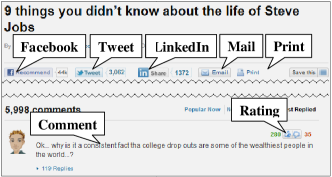
Figure 1: Illustration of post-read actions

We study post-read behavior based on data collected from a major news site in the US that obtains several million visits on a monthly basis. Although this does not represent the entire news reading population in the US and elsewhere in the world, it has a large enough market share to study online news consumption behavior in the US. The site provides various functionalities for users to act after reading an article. Figure 1 shows a portion of a typical news article page. On top are links/buttons that allow a user to share articles on various social media websites such as Facebook, Twitter and LinkedIn. The user can also share the article with others or herself via email or by printing a hard copy. At the bottom portion of the page, the user can leave comments on the article or rate other users comments by thumb-up or thumb-down.

In addition to links/buttons that facilitate post-read actions, most article pages on this site publish a module that recommends interesting article links to users. This module is an important source to create page views on the site and hence recommends article links that maximize overall click-through rates. To estimate the CTR of each article unbiasedly, a small portion of the user visits are shown a random list of articles and the CTR estimated from this small portion of traffic is used to perform our CTR analysis.

2.1 Data

We describe the news data analyzed in this paper.

Source of Data: We collect two kinds of data — (1) all page views on the news site to study post-read actions (these page views are generated via clicks on links to news articles published by the site on the web); and (2) click logs from the module as described earlier. To distinguish link views on the module from page views of news article pages (after clicking article links), we shall refer to the former as “linkview” while the latter is referred to as “pageview”. For instance, using this terminology, pre-read article click-through rate (CTR) is computed as the number of clicks divided by the number of linkviews on the module and post-read Facebook share rate (FSR) is computed as the number of sharing actions divided by the number of pageviews. Post-read action rates of other types can be computed similarly; we focus on the following post-read actions: Facebook share, email, print, comment, and rating.

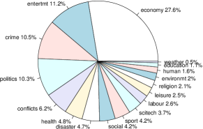
Abbreviation	Full name
economy	economy, business and finance
entertmt	arts, culture and entertainment
crime	crime, law and justice
conflicts	unrest, conflicts and war
disaster	disaster and accident
social	social issue
scitech	science and technology
leisure	lifestyle and leisure
religion	religion and belief
environmt	environmental issue
human	human interest

Figure 2: Distribution of news articles over categories

Data Diversity: The data used in our analysis was collected over a period of several months in 2011. We selected articles that were shown on the module and were clicked at least once, received at least one comment and one post-read action type out of Facebook share, email and print. This gives us approximately 8K articles that were already classified into a hierarchical directory by the publishers. We use the top three levels of the hierarchy for our analysis. The first level of the hierarchy has 17 categories; the distribution of article frequency in these categories is shown in Figure 2. As evident from this figure, news articles published on the site are diverse in nature and provides a good source to study user interaction with online news. We also obtain user demographic information which includes age, gender and geo-location (identified through IP address). All user IDs are anonymized. In total, we have hundreds of millions of pageview events in our data which are sufficient for us to estimate the post-read action rates.

2.2 Pre-Read vs Post-Read

In this section, we investigate the relationship between pre-read (click) and post-read actions. For example, is a highly clicked article also highly shared or commented by users? For each article, we compute the article’s overall click-through rate (CTR) on the module and post-read action rates of different types. In Figure 3, we show the correlation between clicks and other actions types using Pearson’s correlation (the first column or the last row). We observe very low correlation between click rates and other post-read action rates. We also computed the correlations after stratifying articles by categories and found that the correlations are still very low. This lack of correlation is perhaps not surprising: clicks are driven by user’s topical interest in certain articles vs others, while post-click behaviors are inherently conditioned on clicks and hence topical interest. Hence, ranking articles using CTR and other post-click indicators would perhaps lead to different rankings. For instance, if the goal of a news website is to maximize CTR but also ensure a certain minimum number of tweeting and it is possible to predict articles that are more likely to be tweeted, the rankings could be altered based on CTR and tweeting rates to achieve such an objective.

2.3 Correlations among Post-Read Actions

In Figure 3, we also show all pairwise Pearson’s correlations among post-read action types, computed using article-level action rates. We observe positive correlations among various post-read action types; Mail has high correlation with Facebook and print, but not with comment and rating. There is high correlations among Facebook, mail, and print. Not surprisingly, comment and rating are also highly correlated. These provides evidence of being able to leverage correlations among post-read action types to improve estimation.

A word of caution: it is not necessary that correlations will hold when the data is disaggregated at the (user, item) level since our data is observational and subject to various sources of bias. It is not possible to study correlations at the (user, item) level through exploratory analysis due to lack of replicates; we will study this problem rigorously through a modeling approach described in Section 3. The exploratory analysis is shown to provide a flavor of our data (since we are not able to release it due to reasons of confidentiality) and to gain some insights at an aggregate level.

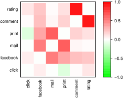
Figure 3: Correlation between different action types (diagonals cells are not of interest)

2.4 Read vs. Post-Read: Private vs. Public

We now compare users’ reading behavior with their post-read behavior. Specifically, is post-read behavior uniform across different article types or user types? Does Joe, a typical young male from California comment and share most of the articles he reads?

To understand this, we use a vector of the fractions of pageviews in different article categories to represent the reading behavior. One can think of this vector as a multinomial probability distribution over categories; i.e., the probability that a random pageview is in a given category. Similarly, marginal post-read behavior of an action type in a category is represented as a vector of fractions of post-read actions of that type in that category. To compare a post-read behavior vector with the reading behavior vector, we compute the element-wise ratio between the two vectors. Figure 4(a) shows these ratios on the log-scale using the top 10 most viewed categories, where the categories are ordered according to the numbers of pageviews they received (highest on the left). All the sample sizes are sufficiently large (with at least tens of thousands of post-read actions) to ensure statistical significance. To help understand this plot, let us consider the green color (i.e., negative value) in the (mail, conflicts) cell for instance. It indicates that a typical user is more likely to read an article about conflicts than email it. In general, if post-read action behavior of users were the same as reading behavior or uniform across news types, the ratios (on log-scale) should be clustered around $0$. Obviously this is not the case for all action types as we see both “hot” and “cold” cells in the plot.

Some interesting tidbits. Users are more likely to read articles about crime, politics and conflicts than to share them with friends via email or on Facebook; they are more likely to read about disaster and science & technology but reluctant to comment on them. When it comes to science and religion, they are eager to share more. They are also more open to leave comments and engage in discussions in a public forum on matters of politics.

We observe an interesting pattern in news consumption. Reading news articles is a private activity, while sharing (Facebook and mail) or expressing opinions (comment and rating) on articles is a public activity and there is difference in a typical user’s public and private activity. Users tend to share articles that earn them social prestige and credit but they do not mind clicking and reading some salacious news occasionally in private.

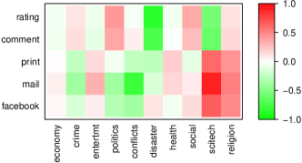
(a) On top level categories

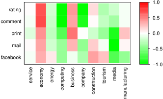
(b) On subcategories of economy

Figure 4: Difference between pageview and post-read actions. This also shows variation of post-read action rates of different types by article categories

2.5 Variation in Post-Read Action Rates at Different Resolutions

The previous subsection showed interesting differences in read and post-read behavior across different article types. In this section, we study variation in post-read action rates by slicing and dicing the data at different resolutions. We note that analysis at some coarse resolution for data obtained through a non-randomized design may not reveal the entire picture; ideally such inferences should be drawn after adjusting for data heterogeneity at the finest, i.e, (user, item) resolution. It is impossible to study variation at this fine resolution through exploratory analysis due to lack of replicates. Our goal in this section is to study variation at resolutions where enough replicates exist. Such an analysis also provide insights into the hardness of predicting action rates and whether sophisticated modeling at fine resolutions is even necessary. For instance, if all science articles behave similarly, it is not necessary to model data at the article level within the science category.

Variation across article categories: To study variation in post-read action rates across article categories, we compute the ratio between the category-specific post-read action rates (i.e., #actions in the category divided by #pageviews in the category) and the global action rate (i.e., total #actions divided by total #pageviews) using the top 10 most viewed categories for each action type. This is exactly what Figure 4(a) and Figure 4(b) show. As we noted earlier, there is variation in action rates at this resolution as evident from the “hot” and “cold” cells.

Variation across user segments: We segment users by age and gender and show post-read action rates for the two genders across different age-groups in Figure 5. Once again we see variation. Some interesting observations: Facebook share rates are highest among young and middle aged users. Users in older age groups tend to mail more but young users tend to share more on Facebook, and also print more. We see females to have surprisingly high share rates and male users tend to comment more on articles. We also include pre-read click actions in this figure and observe that users in older age groups tend to click more; males across all age-groups are more active clickers than females.

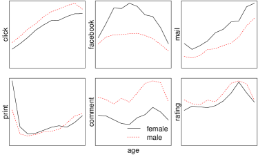
Figure 5: Post-read action rate variation over age-gender segments

Variation within categories and segments: We now dig deeper and analyze variation at the article resolution after stratifying our data by article categories and user segments. High within-category/segment variations at the article level indicate excessive heterogeneity with categories and segments and suggest the need to model the rates at finer resolutions. To study such variation, we leverage the coefficient of variation defined as $\sigma/\mu$, where $\sigma$ is the standard deviation of article action rates within a given category (or category $\times$ user segment) and $\mu$ is the average article action rate in the category (or category $\times$ user segment). $\sigma/\mu$ is a positive number; smaller values indicate less variation. In general, values above $0.2$ are indicative of high variation.

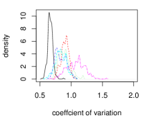
(a) On article categories

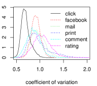
(b) On categories $\times$ age-gender

Figure 6: Density of coefficient of variation

In Figure 6(a) and Figure 6(b), we show the distribution of coefficient of variation with respect to article categories and the cross-product of categories with user age-gender. From these two figures, we can see that all post-read actions have much larger coefficients of variation than click. This means that although there is variation in average post-read behavior across categories and user segments, the variation at the article resolution within each such stratum is high making it difficult to predict article post-read action rates than article click rates based on the category information. Comparing the two figures, we can see that adding user features helps little in terms of reducing coefficients of variation indicating that stratification by user segments does not help in explaining article level variation within each category. Perhaps users with a given (age, gender) segments have different news consumption behavior at the article level.

Our exploratory analysis suggests that predicting post-read actions of any type is harder than estimating CTR. We also see that while using features like article category and user demographics are useful, there is heterogeneity at the article and user resolution that has to be modeled. We also see evidence of positive correlations among post-read action types; it is interesting to study if such correlations can make the estimation task any better. We explore such an approach by modeling all post-read action types simultaneously at the finest (user, item) resolution in section 3.

3 Post-Read Action Prediction

In this section, we present our locally augmented tensor (LAT) model for predicting users’ post-read actions. Given a user, an item (i.e., article) and a post-read action type (e.g., commenting, Facebook sharing), we want to predict whether the user would take the action after reading the item. The main challenges are:

• Data sparsity: Post-read actions are rare events. Most users only have single-digit post-read actions in a month in our dataset. If we further breakdown actions by types, data becomes sparser.

• Diverse behavior across action types: As we saw in Section 2, users behave differently for different action types. For example, the kinds of articles that users like to share are quite different from those that they like to comment on.

To handle data sparsity, an attractive approach is to appropriately pool the action data of a user from all types, so that the action data of one type can be used to improve the prediction performance for another type. However, naive ways of pooling action data that ignore the differences between action types may lead to poor performance, especially for our sparse post-read data.

Problem definition: Consider an online news system with $M$ users, $N$ items and $K$ post-read action types. Let $y_{ijk}$ denote whether user $i$ takes a post-read action of type $k$ on item $j$. If the user takes the action, $y_{ijk}=1$; if the user reads the item and does not take the action, $y_{ijk}=0$; if the user does not read the item, $y_{ijk}$ is unobserved. We also call $y_{ijk}$ the observation or response of user $i$ to item $j$ of type $k$. Each user is associated with a feature vector (e.g., age, gender, geo-location). Each item is also associated with a feature vector (e.g., content categories, words and entities in the item). Because $i$ always denotes a user and $j$ always denotes an item, we slightly abuse our notations by using $\bm{x}_{i}$ to denote the feature vector of user $i$ and $\bm{x}_{j}$ to denote the feature vector of item $j$. Given user features, item features and a set of training observations, our goal is to predict the response of a set of (user, item, action type) triples that do not appear in the training data.

We model the data using variants of factor models. We begin with a review of baseline matrix factorization models and then extend them to address the above challenges.

3.1 Baseline Factor Models

Matrix factorization is a popular method for predicting user-item interaction. User-item interactions can be represented through a $M\times N$ matrix $\mathbf{Y}$, where the value $y_{ij}$ of the $(i,j)^{th}$ entry is the response of user $i$ to item $j$. Notice that this is a matrix with many unobserved (i.e., missing) entries because a user typically does not interact with many items. The main idea of matrix factorization is to obtain two low rank matrices $\mathbf{U}_{M\times F}$ and $\mathbf{V}_{N\times F}$ such that $\mathbf{Y}$ is close to the product $\mathbf{U}\mathbf{V}^{\prime}$ measured in terms of a loss function $l(\mathbf{Y},\mathbf{U}\mathbf{V}^{\prime})$ (e.g. squared-error, logistic). Here $F$ is much smaller than $M$ and $N$. Such a decomposition enables us to predict the unobserved entries in the response matrix.

Each row $\bm{u}_{i}$ of matrix $\mathbf{U}$ is called the factor vector of user $i$, representing his/her latent profile. Similarly, each row $\bm{v}_{j}$ of matrix $\mathbf{V}$ represents the latent profile of item $j$. Intuitively, the inner product $\bm{u}^{\prime}_{i}\bm{v}_{j}$ is a measure of similarity between the profiles of user $i$ and item $j$, representing how much $i$ likes $j$. It is common to also add a bias term $\alpha_{i}$ for each user $i$ to represent his/her average response to items, and a bias term $\beta_{j}$ for each item $j$ to represent its popularity. Then, the response $y_{ij}$ of user $i$ to item $j$ is predicted by $\hat{y}_{ij}=\alpha_{i}+\beta_{j}+\bm{u}^{\prime}_{i}\bm{v}_{j}$.

Let $\ell\ell(y,x)=-\log(1+\exp\{-(2y-1)\,x\})$ denote the logistic log-likelihood for a binary observation $y$. The loss function is given by

$$l(\mathbf{Y},\mathbf{U}\mathbf{V}^{\prime})=-\sum_{\textrm{observed~{}}(i,j)}\ell\ell(y_{ij},\hat{y}_{ij})$$ (1)

Optimizing the loss function in Equation 1 tends to give estimates that overfit sparse data since the number of parameters is too large even for small values of $F$. It is customary to impose penalty (regularization) to avoid overfitting, the most commonly used penalty is to constrain the $L_{2}$ norm of parameters. Thus, we obtain parameter estimates by minimizing

$$\textstyle l(\mathbf{Y},\mathbf{U}\mathbf{V}^{\prime})+\frac{1}{2\sigma^{2}_{\alpha}}\sum_{i}\alpha^{2}_{i}+\frac{1}{2\sigma^{2}_{\beta}}\sum_{j}\beta^{2}_{j}+\frac{1}{2\sigma^{2}_{u}}\sum_{i}||u_{i}||^{2}+\frac{1}{2\sigma^{2}_{v}}\sum_{j}||v_{j}||^{2}$$ (2)

where the $\sigma^{2}_{\cdot}$s are tuning constants. Stochastic gradient descent (SGD) is a popular method to perform such optimization. However, our models involve several tuning constants that are hard to estimate using procedures like cross-validation. Further, SGD also requires tuning learning rate parameters. Thus, we pursue a different estimation strategy for fitting our models by working in a probabilistic framework and using a Monte-Carlo Expectation Maximization (MCEM) procedure. The MCEM approach we follow is both scalable and estimates all parameters automatically through the training data.

3.2 Probabilistic Modeling Framework

Observation model: Matrix factorization can also be interpreted in a probabilistic modeling framework. The given $y_{ij}$s are the observations, based on which we want to estimate the unobserved latent factors $\alpha_{i}$, $\beta_{j}$, $\bm{u}_{i}$ and $\bm{v}_{j}$. For numerical response, it is common to use a Gaussian model.

$$y_{ij}\sim N(\alpha_{i}+\beta_{j}+\bm{u}^{\prime}_{i}\bm{v}_{j},~{}\sigma^{2}_{y}),$$

where $N(\mu,\sigma^{2})$ denote a Gaussian distribution with mean $\mu$ and standard deviation $\sigma^{2}$. For binary response, it is common to use a logistic model.

$$y_{ij}\sim\textit{Bernoulli}(p_{ij})\textrm{ and }\textstyle\log\frac{p_{ij}}{1-p_{ij}}=\alpha_{i}+\beta_{j}+\bm{u}^{\prime}_{i}\bm{v}_{j}.$$

For ease of exposition, we use $y_{ij}\sim\alpha_{i}+\beta_{j}+\bm{u}^{\prime}_{i}\bm{v}_{j}$ to denote that $y_{ij}$ is predicted based on $\alpha_{i}+\beta_{j}+\bm{u}^{\prime}_{i}\bm{v}_{j}$ either using the Gaussian model or the logistic model.

Regression priors: Although $\bm{u}_{i}$ and $\bm{v}_{j}$ are low dimensional, there are still a large number of factors to be estimated from sparse data, which can similarly lead to overfitting. A common approach is to shrink the factors toward zero; i.e., if a factor is not supported by enough data, it’s estimated value should be close to zero. When features are available, we can achieve better performance by shrinking the factors toward values predicted by features, instead of zero. For example, if user $i$ has very few activities in the training data, instead of ensuring $\bm{u}_{i}$ to be close to zero, we predict $\bm{u}_{i}$ using a regression function $G\bm{x}_{i}$, where $G$ is the regression coefficient matrix learned from training data through linear regression. Notice that $\bm{u}_{i}$ is a vector; thus, $G$ is a matrix, instead of a vector. If features are predictive, then we can obtain good $\bm{u}_{i}$ estimates even for users without any training data. Specifically, we assume the following priors.

$$\begin{array}[]{rl rl}\alpha_{i}&\sim N(\bm{g}^{\prime}\bm{x}_{i},\sigma^{2}_{\alpha}),&~{}~{}~{}~{}~{}~{}~{}\bm{u}_{i}&\sim N(G\bm{x}_{i},\sigma^{2}_{u}),\\ \beta_{i}&\sim N(\bm{d}^{\prime}\bm{x}_{j},\sigma^{2}_{\beta}),&~{}~{}~{}~{}~{}~{}~{}\bm{v}_{j}&\sim N(D\bm{x}_{j},\sigma^{2}_{v}).\end{array}$$

Training and prediction: We defer the training algorithm to Section 3.4. Here, we note that this model is a generative model that specifies how the observations $y_{ij}$ are generated according to the latent factors $\alpha_{i}$, $\beta_{j}$, $\bm{u}_{i}$ and $\bm{v}_{j}$, which in turn are generated according to the prior parameters ($\bm{g}$, $G$, $\bm{d}$, $D$ and the $\sigma^{2}_{\cdot}$s). Given a set of observations, we first obtain the maximum likelihood estimate (MLE) of the prior parameters. Then, based on the MLE of prior parameters and the observations, we obtain the posterior mean of $\alpha_{i}$, $\beta_{j}$, $\bm{u}_{i}$ and $\bm{v}_{j}$, which then can be used to predict the response of an unseen $(i,j)$ pair by $\alpha_{i}+\beta_{j}+\bm{u}^{\prime}_{i}\bm{v}_{j}$.

Baseline models: Two straightforward ways of applying matrix factorization to our problem are as follows:

• Separate Matrix Factorization (SMF): Treat observations of $K$ action types as $K$ separate matrices and apply factorization to each of them independently; i.e.,

  $$y_{ijk}\sim\alpha_{ik}+\beta_{jk}+\bm{u}^{\prime}_{ik}\bm{v}_{jk}.$$

• Collapsed Matrix Factorization (CMF): Collapse observations of all types into a single matrix and apply factorization to it; i.e.,

  $$y_{ijk}\sim\alpha_{i}+\beta_{j}+\bm{u}^{\prime}_{i}\bm{v}_{j},$$

  where the right hand side does not depend on type $k$.

Notice that SMF is a strong baseline because for users and items with large number of training samples, their factors can be estimated accurately. For users and items without much training data, their factors can still be predicted by features. Compared to CMF, SMF has $K$ times more factors to be estimated from data and is more sensitive to data sparsity. Although CMF is less sensitive to data sparsity, it ignores the behavioral differences across different action types, which may lead to bias and poor performance.

3.3 Locally Augmented Tensor Model

We now introduce the locally augmented tensor (LAT) model, which addresses data sparsity through tensor factorization, augmented with SMF to model the residuals locally for each action types. We first specify the model and then discuss how it works.

Model specification: The action $y_{ijk}$ that user $i$ takes on item $j$ of type $k$ is modeled as:

$$y_{ijk} \sim\alpha_{ik}+\beta_{jk}+\left<\bm{u}_{i},\bm{v}_{j},\bm{w}_{k}\right>+\bm{u}^{\prime}_{ik}\bm{v}_{jk},$$ (3)

where $\left<\bm{u}_{i},\bm{v}_{j},\bm{w}_{k}\right>=\sum_{\ell}\bm{u}_{i}[\ell]\,\bm{v}_{j}[\ell]\,\bm{w}_{k}[\ell]$ is the tensor product of three vectors $\bm{u}_{i}$, $\bm{v}_{j}$ and $\bm{w}_{k}$, and $\bm{u}_{i}[\ell]$ denotes the $\ell$th element in vector $\bm{u}_{i}$. The intuitive meaning of the factors are as follows.

• $\alpha_{ik}$ is the type-specific bias of user $i$.

• $\beta_{jk}$ is the type-specific popularity of item $j$.

• $\left<\bm{u}_{i},\bm{v}_{j},\bm{w}_{k}\right>$ measures the similarity between user $i$’s global profile $\bm{u}_{i}$ and item $j$’s global profile $\bm{v}_{j}$ weighted by a type-specific weight vector $\bm{w}_{k}$. These profiles are called global because they are not type-specific. Note that this weighted inner product (i.e., tensor product) imposes a constraint when we try to use it to approximate the observations $y_{ijk}$. Specifically, it may not be flexible enough to accurately model post-read actions when there is diverse behavior across action types. However, this constraint in the parametrization helps to avoid overfitting when data is sparse.

• $\bm{u}^{\prime}_{ik}\bm{v}_{jk}$ also measures the similarity between user $i$ and item $j$ for type $k$ and is more flexible than the tensor product. Thus, the residuals that the tensor product does not capture can be captured by this inner product of type-specific user factor $\bm{u}^{\prime}_{ik}$ and item factor $\bm{v}_{jk}$.

To contrast the global factors $\bm{u}_{i},\bm{v}_{j}$, we call the type-specific factors $\bm{u}_{ik},\bm{v}_{jk}$ local factors. Since we augment the tensor product with the inner product of local factors, the resulting model is called the locally augmented tensor model. The priors of the factors are specified as follows.

$$\alpha_{ik} \sim N(\bm{g}_{k}^{\prime}\bm{x}_{ik}+q_{k}\alpha_{i},~{}\sigma_{\alpha,k}^{2}),~{}~{}~{}~{}\alpha_{i}\sim N(0,1)$$ (4)

$$\beta_{jk} \sim N(\bm{d}_{k}^{\prime}\bm{x}_{jk}+r_{k}\beta_{j},~{}\sigma_{\beta,k}^{2}),~{}~{}~{}~{}\beta_{j}\sim N(0,1)$$ (5)

$$\bm{u}_{ik} \sim N(G_{k}\bm{x}_{i},\,\sigma_{uk}^{2}I),~{}~{}~{}~{}\bm{v}_{jk}\sim N(D_{k}\bm{x}_{j},\,\sigma_{vk}^{2}I),$$ (6)

$$\bm{u}_{i} \sim N(\bm{0},\,\sigma_{u0}^{2}I),~{}\bm{v}_{j}\sim N(\bm{0},\,\sigma_{v0}^{2}I),~{}\bm{w}_{k}\sim N(\bm{0},I),$$ (7)

where $\bm{g}_{k}$, $q_{k}$, $\bm{d}_{k}$, $r_{k}$, $G_{k}$ and $D_{k}$ are regression coefficient vectors and matrices similar to those discussed in Section 3.1. These regression coefficients are to be learned from data and provide the ability to make predictions for users or items that do not appear in training data. The factors of these new users or items will be predicted based on their features through regression.

Training and prediction: Given training data $\bm{y}=\{y_{ijk}\}$, the goal of the training process is to learn the latent factors $\bm{\eta}=\{\alpha_{ik},\beta_{jk},\alpha_{i},\beta_{j},\bm{u}_{i},\bm{v}_{j},\bm{w}_{k},\bm{u}_{ik},\bm{v}_{jk}\}$ and prior parameters $\bm{\Theta}=\{\bm{g}_{k},\bm{d}_{k},q_{k},r_{k},G_{k},D_{k},$ the $\sigma_{\cdot}^{2}$s$\}$ (which consists of regression coefficients and variances) from the data $\bm{y}$. The training algorithm will be given later. After training, given an unobserved (user $i$, item $j$, action type $k$) triple, we predict the response as follows. If both user $i$ and item $j$ have some type-$k$ observations in the training data, we just use their learned factors to make a prediction as $\alpha_{ik}+\beta_{jk}+\left<\bm{u}_{i},\bm{v}_{j},\bm{w}_{k}\right>+\bm{u}^{\prime}_{ik}\bm{v}_{jk}$. If user $i$ appears in the training data but has no type-$k$ observation ($\alpha_{i}$ and $\bm{u}_{i}$ are available from training but not $\alpha_{ik}$ and $\bm{u}_{ik}$), then we first predict $\alpha_{ik}$ as $\bm{g}_{k}^{\prime}\bm{x}_{ik}+q_{k}\alpha_{i}$ and $\bm{u}_{ik}$ as $G_{k}\bm{x}_{i}$, and then use Equation 3 to predict the response $y_{ijk}$. Other cases can be handled in a similar manner.

Special cases – SMF and BST: If we set $\alpha_{i}$, $\beta_{j}$, $\bm{u}_{i}$, $\bm{v}_{j}$ and $\bm{w}_{k}$ to zero, we obtain the SMF model (defined in Section 3.1). If we set $\bm{u}_{ik}$ and $\bm{v}_{jk}$ to zero, we obtain the bias-smoothed tensor (BST) model proposed in [4] for a multi-context comment-rating prediction problem; i.e.,

$$y_{ijk}\sim\alpha_{ik}+\beta_{jk}+\left<\bm{u}_{i},\bm{v}_{j},\bm{w}_{k}\right>.$$

Notice that LAT has many latent factors and parameters to be learned. It may be sensitive to overfitting. However, because of the regularization provided by the priors (Equation 4 to 7), overfitting can be prevented when the prior variances are appropriately learned.

3.4 Training Algorithm

Since SMF, CMF and BST are special cases of LAT, we only discuss the training algorithm for LAT. Based on Equations 3 to 7, the joint log-likelihood of $\bm{y}$ and $\bm{\eta}$ given $\bm{\Theta}$ is

$$\begin{split}&\textstyle\log\Pr(\mathbf{y},\bm{\eta}\,|\,\bm{\Theta})=\textrm{ some constant }+\sum_{ijk}\ell\ell(y_{ijk},\hat{y}_{ijk})\\ &\textstyle-\frac{1}{2}\sum_{ik}\big{(}\log\sigma_{\alpha,k}^{2}+(\alpha_{ik}-\bm{g}_{k}^{\prime}\bm{x}_{ik}-q_{k}\alpha_{i})^{2}/\sigma_{\alpha,k}^{2}\big{)}-\frac{1}{2}\sum_{i}\alpha_{i}^{2}\\ &\textstyle-\frac{1}{2}\sum_{jk}\big{(}\log\sigma_{\beta,k}^{2}+(\beta_{jk}-\bm{d}_{k}^{\prime}\bm{x}_{jk}-r_{k}\beta_{j})^{2}/\sigma_{\beta,k}^{2}\big{)}-\frac{1}{2}\sum_{j}\beta_{j}^{2}\\ &\textstyle-\frac{1}{2}\sum_{ik}\big{(}F\log\sigma_{u,k}^{2}+\|\bm{u}_{ik}-G_{k}\bm{x}_{i}\|^{2}/\sigma_{u,k}^{2}\big{)}-\frac{1}{2}\sum_{k}\|\bm{w}_{k}\|^{2}\\ &\textstyle-\frac{1}{2}\sum_{jk}\big{(}F\log\sigma_{v,k}^{2}+\|\bm{v}_{jk}-D_{k}\bm{x}_{j}\|^{2}/\sigma_{v,k}^{2}\big{)}\\ &\textstyle-\frac{1}{2}\sum_{i}(F\,\log\sigma_{u}^{2}+\|\bm{u}_{i}\|^{2}/\sigma_{u0}^{2})-\frac{1}{2}\sum_{j}(F\,\log\sigma_{v}^{2}+\|\bm{v}_{j}\|^{2}/\sigma_{v0}^{2}),\end{split}$$

where $\hat{y}_{ijk}=\alpha_{ik}+\beta_{jk}+\left<\bm{u}_{i},\bm{v}_{j},\bm{w}_{k}\right>+\bm{u}^{\prime}_{i}\bm{v}_{j}$. The goal of training is to obtain MLE of $\bm{\Theta}$; i.e.,

$$\arg\max_{\bm{\Theta}}\Pr(\bm{y}\,|\,\bm{\Theta})=\arg\max_{\bm{\Theta}}\int\Pr(\bm{y},\bm{\eta}\,|\,\bm{\Theta})\,d\bm{\eta},$$

which can be obtained using the MCEM algorithm [3]. The MCEM algorithm iterates between an E-step and an M-step until convergence. Let $\hat{\bm{\Theta}}^{(t)}$ denote the current estimated value of the set of prior parameters $\bm{\Theta}$ at the beginning of the $t$th iteration.

• E-step: We take expectation of the complete data log likelihood with respect to the posterior of latent factors $\bm{\eta}$ conditional on the observed training data $\bm{y}$ and the current estimate of $\bm{\Theta}$; i.e., compute

  $$f_{t}(\bm{\Theta})=E_{\bm{\eta}\sim\Pr\left(\bm{\eta}\,|\,\bm{y},\hat{\bm{\Theta}}^{(t)}\right)}[\log\Pr(\bm{y},\bm{\eta}\,|\,\bm{\Theta})]$$

  as a function of $\bm{\Theta}$, where the expectation is taken over the posterior distribution of $(\bm{\eta}\,|\,\bm{y},\hat{\bm{\Theta}}^{(t)})$, which is not in closed-form, thus, approximated by Monte Carlo mean through Gibbs sampling.

• M-step: We maximize the expected complete data log likelihood from the E-step to obtain updated values of $\bm{\Theta}$; i.e., find $\hat{\bm{\Theta}}^{(t+1)}=\arg\max_{\bm{\Theta}}~{}f_{t}(\bm{\Theta}).$

Note that the actual computation in the E-step is to generate sufficient statistics for computing $\arg\max_{\bm{\Theta}}\,f_{t}(\bm{\Theta})$, so that we do not need to scan the raw data every time when we need to evaluate $f_{t}(\bm{\Theta})$. At the end, we obtain the MLE of $\bm{\Theta}$ modulo local maximums and Monte Carlo errors. We can then use the estimated $\hat{\bm{\Theta}}$ to obtain the posterior mean of the factors $(\bm{\eta}\,|\,\bm{y},\hat{\bm{\Theta}})$ again through Gibbs sampling. See [1] for an example of such an MCEM algorithm.

Computational complexity: We use a Gibbs sampler in the E-step, which is actually highly parallelizable. Take user and item factors for example. Conditional on global factors $\bm{u}_{i},\bm{v}_{j}$, the local factors $\bm{u}_{ik},\bm{v}_{jk}$ for each action type can be sampled in parallel since they are only connected to each other through the global factors. When sampling local factors for each action type, we note that given $v_{jk}$s, the $u_{ik}$s are conditionally independent and can be sampled in parallel (similar assertion holds for $v_{jk}$s). Conditional on local factors, the global factors can also be sampled efficiently since the $\bm{u}_{i}$s and $\bm{v}_{j}$s are conditionally independent. The complexity of sampling a factor vector is at most $O(F^{3})$ and since $F$ is typical small, the E-step is computationally efficient. The major computation in the M-step involves fitting standard linear regressions, which can also be parallelized. Thus, our MCEM algorithm is computationally efficient. We note that this training algorithm is similar to [4, 1] and logistic response can be handled by variational approximation [10]. Thus, we omit the details and will provide links to our code and detailed derivations.

4 Experiments

We evaluate the models presented in Section 3 using post-read data collected from a major online new site. We collected post-read actions from 13,739 users, each of whom has at least 5 actions for at least one facet, to 8,069 items, each of which received at least one post-read action for each type. As a result, we obtain 2,548,111 post-read action events, where each event is identified by (user, facet, item). If the user took an action on the item in the facet, the event is positive or relevant (meaning that the item is relevant to the user in the facet); if the user saw the item but did not take an action in the facet, the event is negative or irrelevant. In this setting, it is natural to treat each (user, facet) pair as a query; the set of events associated with that pair defines the set of items to be ranked with relevance judgments coming from user actions. Notice that it is difficult to use editorial judgments in our setting since different users have different preferences for their news consumption.

Evaluation metrics: We use mean precision at $k$ (P@k) and mean average precision (MAP) as our evaluation metrics, where mean is taken over the test (user, facet) pairs. P@k of a model is computed as follows: For each test (user, facet) pair, we use the model predictions to rank the items seen by the user in that facet and compute the precision at rank $k$, and then average the precision numbers over all the test pairs. MAP is computed in the similar way. To help comparison among different models, we define P@k Lift and MAP Lift over SMF of a model as the lift in P@k and MAP of the model over the SMF model, which is a strong baseline defined in Section 3.1. Take P@k for example; if P@k of a model is $A$ and P@k of SMF is $B$, then the lift is $\frac{A-B}{B}$.

Experimental setup: We create a training set, a tuning set and a test set as follows. For each user, we randomly select one facet in which he/she took some action and put the events associated with this (user, facet) pair into set $\mathcal{A}$ (for tuning and testing). The rest of the (user, facet) pairs form the training set. Recall that each (user, facet) pair represents a query as in standard retrieval tasks. We then put 1/3 of set $\mathcal{A}$ into the tuning set and the rest 2/3 into the test set. The tuning set is used to select the number of latent dimensions of the factor models (i.e., the numbers of dimensions of $\bm{u}_{i},\bm{v}_{j},\bm{w}_{k},\bm{u}_{ik},\bm{v}_{jk}$). Notice that the EM-algorithm used in our paper automatically determines all the model parameters except for the number of latent dimensions. For each model, we only report the test-set performance of the best number of dimensions selected using the tuning set.

The user features used in our experiments consist of age, gender and geo-location identified based on users’ IP addresses. We only consider logged-in users; their user IDs are anonymized and not used in any way. The item features consists of article categories tagged by the publishers and the bag of words in the article titles and abstracts.

Models: We compare the following models:

• LAT: Locally augmented tensor model (Section 3.3).

• BST: Bias-smoothed tensor model, which is a special case of LAT (Section 3.3).

• SMF: Separate matrix factorization (Section 3.1).

• CMF: Collapsed matrix factorization (Section 3.1).

• Bilinear: This model uses the user features $\bm{x}_{i}$ and item features $\bm{x}_{j}$ to predict whether a user would take an action on an item. Specifically,

  $$y_{ijk}\sim\bm{x}^{\prime}_{i}W_{k}\bm{x}_{j},$$

  where $W_{k}$ is the regression coefficient matrix for facet $k$. Notice that this model has a regression coefficient for every pair of an individual user feature and an individual item feature, which is fitted using Liblinear [8] with $L_{2}$ regularization, where the regularization weight is selected using 5-fold cross-validation.

We also compare the above models to a set of baseline IR models. In all of the following IR models, we build a user profile based on the training data by aggregating all the text information of the items on which the user took positive actions. We treat such user profiles as queries and then use different retrieval functions to rank the items. The IR models include:

• COS: Vector space model with cosine similarity.

• LM: The Dirichlet smoothed language model [22].

• BM25: The best variant of Okapi retrieval methods [17].

For the factor models, we note that the Gaussian version gives better MAP values on the tuning set than the logistic version; so, we report the performance of the Gaussian version.

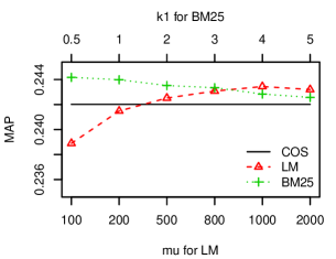
Figure 7: Performance of different IR models

Performance of IR Models: We first compare the baseline IR models in Figure 7. In this figure, we vary parameter $\mu$ for LM and parameter $k_{1}$ for BM25. The other two parameters are set at the recommended default values $k_{3}=1000$ and $b=0.75$ in all the experiments. From this figure, we can see that both LM and BM25 can outperform COS, but the difference is not large. In the following, we use the BM25 with $k_{1}=1$ as the IR model to compare with other learning-based methods.

Overall performance: The precision-recall curves averaged over all (user,facet) pairs in the test data of different models are shown in Figure 8(a), and P@1, P@3, P@5 and MAP are reported in Table 1. Notice that as $k$ increases, the precision drops. It is because post-read actions are rare events; many users do not have 3 or 5 post-read actions in the test set. For example, if a user only had one action and saw at least five items in the test set, his/her P@5 is at most 1/5. To test the significance of the performance difference between two models, we look at P@k and MAP for each individual (user, facet) pair and conduct paired t-test for the two models over all test (user, facet) pairs. The test result is shown in Table 2. In particular, LAT significantly outperforms all other models. We find that the difference between BST and SMF and the difference between CMF and BM25 are insignificant.

We defer the comparison between LAT, BST and SMF to the breakdown analysis below. Here, we note that Bilinear outperforms CMF because CMF completely ignores the behavioral differences among action types. The fact that Bilinear outperforms CMF shows that user and item features have some predictive power, but compared to SMF, these features are not sufficient to capture the behavior of individual users or items. We also note that BM25 is one of the worst performing models probably because it is the only model without supervised learning.

Table 1: Overall performance of different models

	Precision
Model	P@1	P@3	P@5	MAP
LAT	0.3180	0.2853	0.2648	0.3048
BST	0.2962	0.2654	0.2486	0.2873
SMF	0.2827	0.2639	0.2469	0.2910
Bilinear	0.2609	0.2472	0.2350	0.2755
CMF	0.2301	0.2101	0.2005	0.2439
BM25	0.2256	0.2247	0.2207	0.2440

Table 2: Paired t-test result. Note that smaller level values represent stronger significance.

Comparison			Significance level
LAT	>	BST	0.05 (P@1),  $10^{-4}$ (P@3, P@5, MAP)
		Rest	$10^{-4}$ (all metrics)
BST	$\approx$	SMF	insignificant
BST	>	Bilinear	$10^{-3}$ (all metrics)
SMF	>	Bilinear	0.05 (P@1),  $10^{-3}$ (P@3, P@5, MAP)
BST	>	CMF	$10^{-4}$ (all metrics)
SMF		BM25
Bilinear	>	CMF	$10^{-3}$ (all metrics)
		BM25
CMF	$\approx$	BM25	insignificant

Breakdown by facets: In Table 3, we break the test data down by facets and report P@1 for different models; the results for other metrics are similar. Here, we focus on the comparison between LAT, BST and SMF. Starting with BST vs. SMF, we see that BST outperforms SMF for the first three facets but underperforms for the last two facets. We note that the first three facets have more events in our dataset than the last two. The advantage of BST over SMF is that it has global factors; thus, the training actions in one facet are utilized to predict the test actions in other facets through the correlation among facets. However, BST is less flexible than SMF. In particular, it is not flexible enough to capture the differences among facets; thus, it is forced to fit some facets better than others. As expected, it fits the actions in facets with more data better than those with less data. LAT addresses this problem by adding facet-specific factors ($\bm{u}_{ik}$ and $\bm{v}_{jk}$) to model the residuals of BST. As can be seen, LAT uniformly outperforms BST. It also outperforms SMF except for Mail. The fact that SMF and Bilinear have the same performance for Mail suggests the difficulty of using latent factors to improve accuracy. Since LAT has more factors than SMF, it has a higher chance of overfitting.

Table 3: P@1 broken down by Facets

	Facet
Model	Comment	Thumb	Facebook	Mail	Print
LAT	0.3477	0.3966	0.2565	0.2069	0.2722
BST	0.3310	0.3743	0.2457	0.1936	0.1772
SMF	0.2949	0.3408	0.2306	0.2255	0.2532
Bilinear	0.2837	0.2947	0.2328	0.2255	0.1709
CMF	0.2990	0.2905	0.1638	0.1114	0.1203
BM25	0.2726	0.3198	0.1509	0.1061	0.0886

Breakdown by user activity levels: In Figure 8(b) and 8(c), we break test users down by their activity levels in terms of the numbers of post-read actions that they took in the training data. Here, our focus is also on comparing LAT and BST to SMP. Each curve represent the P@1 Lift or MAP Lift of each model over the SMF model as a function of the user activity level specified on the x-axis. As can be seen, LAT almost uniformly outperforms all other models. For users with low activity levels (0-5), there is almost no difference between LAT, BST and SMF because they all lack data and the predictions are mostly based on features. For users who took 5-50 post-read actions, we see the largest advantage of using LAT.

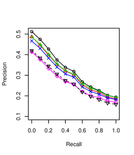
(a) Precision-recall curves

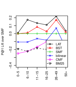
(b) P@1 by user activity levels

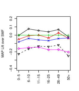
(c) MAP by user activity levels

Figure 8: Performance of different models

Perceived differences among facets: In Table 4, we show some examples of the result of multi-faceted news ranking. On the top half of the table, we show top-ranked articles for an average user. On the bottom half, we show top-ranked articles for males with ages between 41 and 45. From this table, we can see that different facets have very different ranking results. For example, in the Facebook and Mail facets, many health-related articles are highly ranked. But for the Comment facet, political articles are usually preferred. Furthermore, if we compare the males in the middle age with the overall population, we also see notable differences. For example, although both populations have health-related articles in the Mail facet, middle-age males tend to mail more cancer-related articles. These differences confirm the need for personalized multi-facet ranking and our proposed method can address this need in a principled way.

Facebook	Mail	Comment
Overall population
US weather tornado Japan disaster aid	Teething remedies pose fatal risk to infants	US books Michelle Obama
Eight ways monsanto is destroying our health	US med car seats children	US Obama immigration
Teething remedies pose fatal risk to infants	Super women mom soft wins may live longer	US exxon oil prices
New zombie ant fungi found	Tips for a successful open house	Harry Reid: republicans fear tea party
Indy voters would rather have Charlie Sheen …	Painless diabetes monitor talks to smartphone	Obama to kick off campaign this week
For male at age 41 to 45
Oxford English dictionary added new words	Richer white women more prone to melanoma	Israel troubling tourism
US exxon oil prices	Obesity boost aggressive breast cancer in older women	Israel palestinians
Children make parents happy eventually	US med car seats children	USA election Obama
Qatar Saudi politics Internet	Are coffee drinkers less prone to breast cancer	US books Michelle Obama
Lawmakers seek to outlaw prank calls	Short course of hormone therapy boosts prostate cancer	Levi Johnston to write memoir

Table 4: Examples of multi-faceted news ranking. Only the titles of the news articles are shown.

5 Related Work

Algorithmic news recommendation has received considerable attention recently. Traditional recommendation approaches include content-based filtering and collaborative filtering techniques [24, 18, 11]. These techniques have been successfully applied to applications like movie or product recommendation [18, 14]. In particular, matrix factorization based collaborative filtering, which belongs to the family of latent factor models, have achieved the state-of-the-art accuracy [11]. Recently, these methods have been adapted for news recommendation. For example, [9] studied information novelty using content-based methods. In [6], collaborative filtering was leveraged in an online news recommendation system. Hybrid approaches which combine both content-based and collaborative methods are also studied in news recommendation recently [13]. In the news domain, the existing work mainly ranks articles using clicks as the metric. Some recent work starts looking into other metrics such as social sharing [5]. To the best of our knowledge, little prior work has studied the news recommendation in a multi-faceted view, which becomes natural along with the popularity of Web 2.0. In our work, we define facets according to post-read actions and provide detailed analysis which shows the importance of multi-faceted news ranking. Furthermore, a novel matrix factorization based method to jointly model multi-type post-read actions is proposed.

Our work is related to faceted search [21, 23, 7]. The goal of faceted search is to use facet metadata of a domain to help users narrow their search results along different dimensions. In the most recent TREC Blog track 2009 [15], a special track of “faceted blog distillation” is initiated and the task of this track is to find results relevant to a single facet of a query such as “opinionated” articles in the blog collection. In these types of work, facets are metadata related to contents. The facets in our definition are based on user post-read actions and our multi-faceted ranking is to help users quickly get interesting news articles according to their preferred actions. Thus our work provides a novel angle to define facets.

The technique used in our paper is closely related to latent factor models such as matrix factorization or tensor decomposition. For example, singular value decomposition (SVD) based methods [11], tensor-based methods [16], and collaborative competitive filtering [20] all belong to this family. All these methods did not consider post-read actions. In particular, our technique is related to the collective matrix factorization (CMF) [19] and bias-smoothed tensor (BST) model [4]. As compared in our experiments, our models are better than these existing ones in exploring the correlations among different post-read facets.

6 Conclusion

Jointly mining and modeling post-read actions of multiple types has not been previously studied in the literature. We conducted a rigorous study on post-read behavior on Yahoo! News with action types like facebook share, commenting, rating that users engage in after reading an article. Through data analysis, we found some interesting patterns in news consumption when it comes to read and post-read behavior. Reading articles is private, post-read behavior like sharing and commenting are more public. Users tend to differ in interesting ways in their public and private behavior when interacting with news. We also saw huge variation in post-read action rates at the article resolution relative to classical measures like click-rates that are used in recommending articles, perhaps providing a plausible explanation of why such engagment metrics have not been incorporated into news recommendation algorithms before. However, we found positive correlations among different action types and were able to exploit these through a novel factor model called Locally Augmented Tensor (LAT) to improve predictive performance of post-read action rates. This opens the door to incorporate post-read engagement behavior in creating new products/modules on news sites online. We plan to explore such possibilities in the future.

References

- [1] D. Agarwal and B.-C. Chen. Regression-based latent factor models. In KDD, 2009.
- [2] D. Agarwal, B.-C. Chen, P. Elango, N. Motgi, S.-T. Park, R. Ramakrishnan, S. Roy, and J. Zachariah. Online models for content optimization. In NIPS, 2008.
- [3] J. Booth and J. Hobert. Maximizing generalized linear mixed model likelihoods with an automated monte carlo EM algorithm. J.R.Statist. Soc. B, 1999.
- [4] B.-C. Chen, J. Guo, B. Tseng, and J. Yang. User reputation in a comment rating environment. In KDD, 2011.
- [5] P. Cui, F. Wang, S. Liu, M. Ou, S. Yang, and L. Sun. Who should share what?: item-level social influence prediction for users and posts ranking. In SIGIR, 2011.
- [6] A. S. Das, M. Datar, A. Garg, and S. Rajaram. Google news personalization: scalable online collaborative filtering. In WWW, 2007.
- [7] S. T. Dumais. Faceted search. In Encyclopedia of Database Systems. 2009.
- [8] R.-E. Fan, K.-W. Chang, C.-J. Hsieh, X.-R. Wang, and C.-J. Lin. Liblinear: A library for large linear classification. JMLR, 2008.
- [9] E. Gabrilovich, S. T. Dumais, and E. Horvitz. Newsjunkie: providing personalized newsfeeds via analysis of information novelty. In WWW, 2004.
- [10] T. S. Jaakkola and M. I. Jordan. Bayesian parameter estimation via variational methods. Statistics and Computing, 2000.
- [11] Y. Koren. Factorization meets the neighborhood: a multifaceted collaborative filtering model. In KDD, 2008.
- [12] L. Li, W. Chu, J. Langford, and R. E. Schapire. A contextual-bandit approach to personalized news article recommendation. In WWW, 2010.
- [13] L. Li, D. Wang, T. Li, D. Knox, and B. Padmanabhan. Scene: a scalable two-stage personalized news recommendation system. In SIGIR, 2011.
- [14] G. Linden, B. Smith, and J. York. Amazon.com recommendations: Item-to-item collaborative filtering. IEEE Internet Computing, 7(1), 2003.
- [15] C. Macdonald, I. Ounis, and I. Soboroff. Overview of the trec 2009 blog track. 2009.
- [16] S. Rendle, Z. Gantner, C. Freudenthaler, and L. Schmidt-Thieme. Fast context-aware recommendations with factorization machines. In SIGIR, 2011.
- [17] S. E. Robertson, S. Walker, S. Jones, M. M.Hancock-Beaulieu, and M. Gatford. Okapi at TREC-3. In D. K. Harman, editor, The Third Text REtrieval Conference (TREC-3), 1995.
- [18] B. M. Sarwar, G. Karypis, J. A. Konstan, and J. Riedl. Item-based collaborative filtering recommendation algorithms. In WWW, 2001.
- [19] A. P. Singh and G. J. Gordon. Relational learning via collective matrix factorization. In KDD, 2008.
- [20] S.-H. Yang, B. Long, A. J. Smola, H. Zha, and Z. Zheng. Collaborative competitive filtering: learning recommender using context of user choice. In SIGIR, 2011.
- [21] K.-P. Yee, K. Swearingen, K. Li, and M. Hearst. Faceted metadata for image search and browsing. In CHI, 2003.
- [22] C. Zhai and J. Lafferty. A study of smoothing methods for language models applied to ad hoc information retrieval. In SIGIR, 2001.
- [23] L. Zhang and Y. Zhang. Interactive retrieval based on faceted feedback. In SIGIR, 2010.
- [24] Y. Zhang and J. Koren. Efficient bayesian hierarchical user modeling for recommendation system. In SIGIR, 2007.