QCD in heavy ion collisions

Abstract

These lectures provide a modern introduction to selected topics in the physics of ultrarelativistic heavy ion collisions which shed light on the fundamental theory of strong interactions, the Quantum Chromodynamics. The emphasis is on the partonic forms of QCD matter which exist in the early and intermediate stages of a collision — the colour glass condensate, the glasma, and the quark–gluon plasma — and on the effective theories that are used for their description. These theories provide qualitative and even quantitative insight into a wealth of remarkable phenomena observed in nucleus–nucleus or deuteron–nucleus collisions at RHIC and/or the LHC, like the suppression of particle production and of azimuthal correlations at forward rapidities, the energy and centrality dependence of the multiplicities, the ridge effect, the limiting fragmentation, the jet quenching, or the dijet asymmetry.

1 Introduction

With the advent of the high–energy colliders RHIC (the Relativistic Heavy Ion Collider operating at RHIC since 2000) and the LHC (the Large Hadron Collider which started operating at CERN in 2008), the physics of relativistic heavy ion collisions has entered a new era: the energies available for the collisions are high enough — up to 200 GeV per interacting nucleon pair at RHIC and potentially up to 5.5 TeV at the LHC (although so far one has reached ‘only’ 2.76 TeV) —- to ensure that new forms of QCD matter, characterized by high parton densities, are being explored by the collisions. These new forms of matter refer to both the wavefunctions of the incoming nuclei, prior to the collision, which develop high gluon densities leading to colour glass condensates, and the partonic matter produced in the intermediate stages of the collision, which is expected to form a quark–gluon plasma. The asymptotic freedom property of QCD implies that these high–density forms of matter are weakly coupled (at least in so far as their bulk properties are concerned) and hence can be studied via controlled calculations within perturbative QCD. But such studies remain difficult and pose many challenges to the theorists: precisely because of their high density, these new forms of matter are the realm of collective, non–linear phenomena, whose mathematical description often transcends the ordinary perturbation theory. Moreover, there are also phenomena (first revealed by the experiments at RHIC) which seem to elude a weak–coupling description and call for non–perturbative techniques.

These challenges stimulated new ideas and the development of new theoretical tools aiming at a fundamental understanding of QCD matter under extreme conditions : high energy, high parton densities, high temperature. The ongoing experimental programs at RHIC and the LHC provide a unique and timely opportunity to test such new ideas, constrain or reject models, and orient the theoretical developments. Over the last decade, the experimental and theoretical efforts have gone hand in hand, leading to a continuously improving physical picture, which is by now well rooted in QCD. The purpose of these lectures is to provide an introduction to this physical picture, with emphasis on those aspects of the dynamics for which we are confident to have a reasonably good (although still far from perfect) understanding from first principles, i.e. from the Lagrangian of Quantum Chromodynamics. These aspects concern the partonic stages of a heavy ion collision, at sufficiently early times. These are also the stages to which refers most of the experimental and theoretical progress over the last decade.

2 Stages of a heavy ion collision: the case for effective theories

The theoretically motivated space–time picture of a heavy ion collision (HIC) is depicted in fig:HIC. This illustrates the various forms of QCD matter intervening during the successive phases of the collision:

1. Prior to the collision, and in the center-of-mass frame (which at RHIC and the LHC is the same as the laboratory frame), the two incoming nuclei look as two Lorentz–contracted ‘pancakes’, with a longitudinal extent smaller by a factor $\gamma\sim 100$ (the Lorentz boost factor) than the radial extent in the transverse plane. As we shall see, these ‘pancakes’ are mostly composed with gluons which carry only tiny fractions $x\ll 1$ of the longitudinal momenta of their parent nucleons, but whose density is rapidly increasing with $1/x$. By the uncertainty principle, the gluons which make up such a high–density system carry relatively large transverse momenta. A typical value for such a gluon in a Pb or Au nucleus is $k_{\perp}\simeq 2$ GeV for $x=10^{-4}$. By the ‘asymptotic freedom’ property of QCD, the gauge coupling which governs the mutual interactions of these gluons is relatively weak. This gluonic form of matter, which is dense and weakly coupled, and dominates the wavefunction of any hadron (nucleon or nucleus) at sufficiently high energy, is universal — its properties are the same form all hadrons. It is known as the colour glass condensate (CGC).

2. At time $\tau=0$, the two nuclei hit with each other and the interactions start developing. The ‘hard’ processes, i.e. those involving relatively large transferred momenta $Q\gtrsim 10$ GeV, are those which occur faster (within a time $\tau\sim 1/Q$, by the uncertainty principle). These processes are responsible for the production of ‘hard particles’, i.e. particles carrying transverse energies and momenta of the order of $Q$. Such particles, like (hadronic) jets, direct photons, dilepton pairs, heavy quarks, or vector bosons, are generally the most striking ingredients of the final state and are often used to characterize the topology of the latter — one speaks about ‘a dijet event’, cf. fig:events left, or ‘a photon–jet’ event, cf. fig:events right.

   

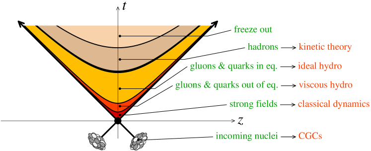
   Figure 1: Schematic representation of the various stages of a HIC as a function of time $t$ and the longitudinal coordinate $z$ (the collision axis). The ‘time’ variable which is used in the discussion in the text is the proper time $\tau\equiv\sqrt{t^{2}-z^{2}}$, which has a Lorentz–invariant meaning and is constant along the hyperbolic curves separating various stages in this figure.

3. At a time $\tau\sim 0.2$ fm/c, corresponding to a ‘semi-hard’ transverse momentum scale $Q\sim 1$ GeV, the bulk of the partonic constituents of the colliding nuclei (meaning the gluons composing the respective CGCs) are liberated by the collision. This is when most of the ‘multiplicity’ in the final state is generated; that is, most of the hadrons eventually seen in the detectors are produced via the fragmentation and the hadronisation of the initial–state gluons liberated at this stage. But before ending up in the detectors, these partons undergo a complex evolution. Just after being liberated, they form a relatively dense medium, whose average density energy in Pb+Pb collisions at the LHC is estimated as $\varepsilon\gtrsim 15$ GeV/fm³; this is about 10 times larger than the density of nuclear matter and 3 times larger than in Au+Au collisions at RHIC. This non–equilibrium state of partonic matter, which besides its high density has also other distinguished features to be discussed later, is known as the glasma.

     

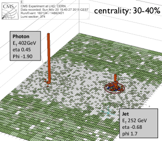
   Figure 2: A couple of di–jets events in Pb+Pb collisions at ATLAS (left) and CMS (right).

4. If the produced partons did not interact with each other, or if these interactions were negligible, then they would rapidly separate from each other and independently evolve (via fragmentation and hadronization) towards the final–state hadrons. This is, roughly speaking, the situation in proton–proton collisions. But the data for heavy ion collisions at both RHIC and the LHC exhibit collective phenomena (like the ‘elliptic flow’ to be discussed later) which clearly show that the partons liberated by the collision do actually interact with each other, and quite strongly. A striking consequence of these interactions is the fact that this partonic matter rapidly approaches towards thermal equilibrium : the data are consistent with a relatively short thermalization time, of order $\tau\sim 1$ fm/c. This is striking since it requires rather strong interactions among the partons, which can compete with the medium expansion: these interactions have to redistribute energy and momentum among the partons, in spite of the fact that the latter separate quite fast away from each other. Such a rapid thermalization seems incompatible with perturbative calculations at weak coupling and represents a main argument in favour of a new paradigm: the dense partonic matter produced in the intermediate stages of a HIC may actually be a strongly coupled fluid.

5. The outcome of this thermalization process is the high–temperature phase of QCD known as the quark–gluon plasma. The abundant production and detailed study of this phase is the Holy Grail of the heavy ion programs at RHIC and the LHC. The existence of this phase is well established via theoretical calculations on the lattice, but its experimental production within a HIC is at best ephemeral: the partonic matter keeps expanding and cooling down (which in particular implies that the temperature is space and time dependent, i.e. thermal equilibrium is reached only locally) and it eventually hadronizes — the ‘coloured’ quark and gluons get trapped within colourless hadrons. Hadronization occurs when the (local) temperature becomes of the order of the critical temperature $T_{c}$ for deconfinement, known from lattice QCD studies as $T_{c}\simeq 150\div 180$ MeV. In Pb+Pb collisions at the LHC, this is estimated to happen around a time $\tau\sim 10$ fm/c.

6. For larger times $10\lesssim\tau\lesssim 20$ fm/c, this hadronic system is still relatively dense, so it preserves local thermal equilibrium while expanding. One then speaks of a hot hadron gas, whose temperature and density are however decreasing with time.

7. Around a time $\tau\sim 20$ fm/c, the density becomes so low that the hadrons stop interacting with each other. That is, the collision rate becomes smaller than the expansion rate. This transition between a fluid state (where the hadrons undergo many collisions) and a system of free particles is referred to as the freeze–out. From that moment on, the hadrons undergo free streaming until they reach the detector. One generally expects that the momentum distribution of the outgoing particles is essentially the same as their thermal distribution within the fluid, towards the late stages of the expansion, just before the freeze–out. This assumption appears to be confirmed by the data: the particle spectra as measured by the detectors can be well described as thermal (Maxwell–Boltzmann) distributions, with only few free parameters, like the fluid temperature and velocity at the time of freeze–out. This is generally seen as an additional argument in favour of thermalization, but one must be cautious on that, since the mechanism of hadronisation itself can lead to spectra which are apparently thermal. As a matter of fact, the freeze–out temperature extracted from the ratios of particle abundances at RHIC appears to be the same, $T_{f}\simeq 170$ MeV, in both Au+Au and p+p collisions, while of course no QGP phase is expected in p+p.

Although extremely schematic, this simple enumeration of the various stages of a HIC already illustrates the variety and complexity of the forms of matter traversed by the QCD matter liberated by the collision on its way to the detectors. In principle, all these forms of matter and their mutual transformations admit an unambiguous theoretical description in the framework of Quantum Chromodynamics, which is the fundamental theory of strong interactions. But although this theory exists with us for about 40 years, it is still far from having delivered all its secrets. Indeed, in spite of the apparent simplicity of its Lagrangian, which looks hardly more complicated than that of the quantum electrodynamics (the theory of photons and electrons), the QCD dynamics is considerably richer and more complicated — which is why it can accommodate so many phases! What renders the theoretical study of HIC’s so difficult is the extreme complexity of the relevant forms of hadronic matter, characterized by high (parton or hadron) densities and strong collective phenomena. For a theorist, the most efficient way to try and organize this complexity is to build effective theories.

An ‘effective theory’ should not be confused with a ‘model’: its main purpose is not to provide a heuristic description of the data using some physical guidance together with a set of free parameters. Rather, it aims at a fundamental understanding and its construction is always guided by the underlying fundamental theory — here, QCD. Specifically, an effective theory is a simplified version of the fundamental theory which includes the ‘soft’ (i.e. low energy and momentum) degrees of freedom (d.o.f.) required for the description of the physical phenomena occurring at a relatively large space–time scale, but ignores the ‘hard’ d.o.f. with higher energies and momenta. More precisely, the hard modes cannot be totally ignored — they interact with the soft modes and thus affect the properties of the effective theory —, rather they are ‘integrated out’ via some coarse–graining (or ‘renormalization group’) procedure, which can be perturbative or non–perturbative.

If the coupling is weak ($g\ll 1$), the ‘hard–soft’ interactions can be treated in perturbation theory and then the effective theory emerges as a controlled approximation to the original theory. This generally amounts to computing Feynman graphs with hard loop momenta and soft external legs. By the uncertainty principle, the hard modes are localized on short space–time distances, so their net effect is to provide quasi–local vertices, or ‘parameters’ — like effective masses and couplings — in the effective Lagrangian for the soft modes. But even at weak coupling, one often has to deal with a large, or even infinite, number of Feynman graphs at any given order in $g$, because the contributions due to individual graphs are enhanced by the large disparity of scales between the hard and soft d.o.f. and/or by the high density of medium constituents. This is where the effective theory is most useful: it allows us to ‘resum’ (modulo some approximations) a large number of Feynman graphs of the original field theory and replace their effects by a small number of ‘parameters’ in the effective Lagrangian.

When the coupling is relatively strong, $g\gtrsim 1$, standard perturbation theory (the expansion in powers of $g$) is bound to fail and the construction of effective theories becomes more problematic. So long as the coupling is just moderately strong, say $g\sim\mathcal{O}{(1)}$, there is still hope that some insightful resummations of the perturbation theory, as based on the proper identification of the relevant d.o.f., may reasonably work — we shall later encounter some examples in that sense. If, in some regime, the coupling happens to be even stronger, perturbation theory brings no guidance anymore, and there is no systematic method to construct effective theories. They can merely be postulated on the basis of general physical considerations, like the symmetries of the fundamental theory. In such a case, the effective masses or coupling constants are generally treated as free parameters, to be matched against the data or, in some cases, against lattice QCD calculations. Effective theories may also emerge for rather deep and unexpected reasons, as we shall see on the example of the gauge/string duality later on.

If in the previous discussion we mentioned both weak and strong coupling scenarios, is because in QCD — and indeed in any of the fundamental field theories in Nature — the coupling ‘constant’ is not fixed: it ‘runs’ with the typical momenta exchanged in the interactions, meaning that it is different when probing the physics on different space–time scales. What is essential about QCD is the property of asymptotic freedom : the fact that the coupling becomes weaker on shorter distances, or with increasing momentum transfer. Given our experience with electromagnetism, this property may look counterintuitive. In QED, the electric charge of the nucleus inside an atom is well known to be screened by the surrounding electron cloud, so that the atom appears electrically neutral from far away. Similarly, the electric charge of an electron is screened by electron–positron virtual pairs which pump up from the vacuum, with the result that the effective charge $\alpha_{\rm e.m.}(R)\equiv e^{2}(R)/4\pi$ decreases with the distance $R$ from the electron. But in QCD, there is anti–screening: the effective colour charge of a quark or gluon, as measured by its coupling ‘constant’ $\alpha_{s}(R)\equiv g^{2}(R)/4\pi$, increases with $R$ or with decreasing the transferred momentum $Q$. (Recall that $Q\sim 1/R$ by the uncertainty principle.) Specifically, one has $\alpha_{s}(Q^{2})\simeq 0.1$ when $Q=100$ GeV (the typical scale for electroweak physics and also for hadronic jets at the LHC). This ‘asymptotic freedom’ is, of course, the ultimate reason behind the success story of perturbative QCD in relation with ‘hard’ processes. It also justifies the use of perturbation theory for integrating out the ‘hard’ d.o.f. in the construction of effective theories for the ‘soft’ ones.

But there is also the reverse of the medal: with decreasing $Q$ below 100 GeV, the QCD coupling is increasing, albeit slowly, according to

$$\alpha_{s}(Q^{2})\,\equiv\,\frac{g^{2}(Q^{2})}{4\pi}\,=\,\frac{4\pi N_{c}}{(11N_{c}-2N_{f})\ln({Q^{2}}/{\Lambda_{{\rm QCD}}^{2}})}\,,$$ (1)

so that e.g. $\alpha_{s}(Q^{2})\simeq 0.4$ when $Q=2$ GeV. Formally, run predicts that the coupling diverges when $Q=\Lambda_{{\rm QCD}}$, but this equation cannot be trusted for $Q\lesssim 1$ GeV, as it has been obtained in perturbation theory. The fate of the QCD coupling for $Q\sim\Lambda_{{\rm QCD}}$ is still under debate, but various non–perturbative approaches suggest that $\alpha_{s}(Q^{2})$ should (roughly) saturate at a value close to one. For all purposes, this is very strong coupling (e.g. it corresponds to $g\simeq 3$).

After this digression through the general scope of an effective theory and the QCD running coupling, let us return to the main stream of our presentation, namely, the phases of QCD as probed in a HIC. Some key ideas, that will be succinctly mentioned here and developed in more detail in the remaining part of these lectures, are as follows:

(i) The different stages of a HIC involve different forms of hadronic matter with specific active degrees of freedom. Their theoretical description requires different effective theories.

(ii) During the early stages of the collision — the colour glass condensate and the glasma — the parton density is very high, the typical transverse momenta are semi–hard (a few GeV), and the QCD coupling is moderately weak, say $\alpha_{s}\sim 0.3$. In this case, perturbation theory is (at least, marginally) valid, but it goes beyond a straightforward expansion in powers of $\alpha_{s}$. The construct the corresponding effective theory, one needs to resum an infinite class of Feynman graphs which are enhanced by high–energy and high gluon density effects. This has been done in the recent years, led to a formalism — the CGC effective theory — which offers a unified description from first principles for both the nuclear wavefunctions prior to the collision and the very early stages of the collision. A key ingredient in this construction is the proper recognition of the relevant d.o.f. : quasi–classical colour fields. The concept of field is indeed more useful in this high–density environnement than that of particle, since the phase–space occupation numbers are large ($\gg 1$), meaning that the would–be ‘particles’ overlap with each other and thus form coherent states, which are more properly described as classical field configurations.

(iii) At later stages, the partonic matter expands, the phase–space occupation numbers decrease, and the concept of particle becomes again meaningful: the classical fields break down into particles. If these particles are weakly coupled (as one may expect by continuity with the previous stages), then their subsequent evolution can be described by kinetic theory. This is an effective theory which emerges under the assumption that the mean free path between two successive collisions is much longer than any other microscopic scale (like the duration of a collision or the Compton wavelength $\lambda=1/k_{\perp}$ of a particle). Over the last years, kinetic theory has been extensively derived from QCD at weak coupling, but the results appear to be deceiving: for instance, they cannot explain the rapid thermalization suggested by the data at RHIC and the LHC. (The thermalization times predicted by perturbative QCD are much larger, $\tau\gtrsim 10~{}$fm/c.) Several alternative solutions have been proposed so far, but the final outcome is still unclear. One of these proposals is that the softer modes, which keep large occupation numbers and should be better described as classical fields, become unstable due to the anisotropy in the momentum distribution of the harder particles (which in turns follows from the disparity between longitudinal and transverse expansions). But numerical simulations of the coupled system soft fields–hard particles leads to thermalization times which are still too large. Another suggestion is that the partonic matter is (moderately) strongly coupled — the QCD coupling could indeed become larger, because of the system being more dilute. In such a scenario, a candidate for an effective theory is the AdS/CFT correspondence, to be discussed later.

(iv) Assuming (local) thermal equilibrium, and hence the formation of a quark–gluon plasma (QGP), the question is whether this plasma is weakly or strongly coupled. The maximal temperature of this plasma, as estimated from the average energy density, should be around $T\sim 500\div 600$ MeV; so the respective coupling is moderately strong: $\alpha_{s}\sim 0.3\div 0.4$ or $g\sim 1.5\div 2$. The thermodynamic properties (like pressure or energy density) of a QGP at global thermal equilibrium within this range of temperatures are by now well known from numerical calculations on a lattice and can serve as a baseline of comparison for various effective theories. If the coupling is weak, one has to use the Hard Thermal Loop effective theory (HTL), a version of the kinetic theory which describes the long–range (or ‘soft’) excitations of the QGP. This effective theory lies at the basis of a physical picture of the QGP as a gas of weakly–coupled quasi–particles — quarks or gluons with temperature–dependent effective masses and couplings. Using this picture as a guideline for reorganizations of the perturbation theory, one has been able to reproduce the lattice data quite well. Thus, the thermodynamics appears to be consistent with a weak–coupling picture for the QGP, although this picture is considerably more complicated than that emerging from naive perturbation theory (the strict expansion in powers in $g$). Yet, this is not the end of the problem, as we shall see.

(v) The QGP created in the intermediate stages of a HIC is certainly not in global thermal equilibrium, but only in a local one: it keeps expanding. Under very general assumptions, the effective theory describing this flow is hydrodynamics. The corresponding equations of motion are simply the conservation laws for energy, momentum, and other conserved quantities (like the electric charge or the baryonic number), and as such they are universally valid. But these equations also involve ‘parameters’, like the viscosities, which describe dissipative phenomena occurring during the flow and which depend upon the specific microscopic dynamics. The values of these parameters are very different at weak vs. strong coupling. A meaningful way to characterize the strength of dissipation is via the dimensionless viscosity–over–entropy-density ratio $\eta/s$. (This ratio is dimensionless when using natural units; otherwise it has the dimension of $\hbar$.) Remarkably, the elliptic flow data at RHIC and the LHC to be later discussed suggest a very small value for this ratio, which is inconsistent with the present calculations at weak coupling, based on kinetic theory. On the other hand, such a small ratio is naturally emerging at strong coupling, as shown by calculations within the AdS/CFT correspondence. The smallness of $\eta/s$ represents so far the strongest argument in favour of a strongly coupled quark–gluon plasma (sQGP). This may look contradictory with the previous conclusions drawn from thermodynamics. But one should remember that the QCD coupling depends upon the relevant space–time scale and that hydrodynamics refers to the long–range behaviour of the fluid, as encoded in its softest modes. By contrast, thermodynamics is rather controlled by the hardest modes — those with typical energies and momenta of the order of the (local) temperature. So, it is not inconceivable that a same system look effectively weakly coupled for some phenomena and strongly coupled for some others.

(vi) Another strategy for studying the hadronic matter produced in a HIC refers to the use of hard probes. These are particles with large transverse energies (say, $E_{\perp}\gtrsim 20$ GeV at the LHC), which are produced in the very first instants of a collision and then cross the QCD matter liberated at later stages along their way towards the detector. Some of these particles, like the (direct) photons and the dilepton pairs, do not interact with this matter and hence can be used a baseline for comparaisons. But other particles, like quarks, gluons, and the jets initiated by them, do interact, and by measuring the effects of these interactions — say, in terms of energy loss, or the suppression of multi–particle correlations — one can infer informations about the properties of the matter they crossed. The RHIC data have demonstrated that semi–hard partons can lose a substantial fraction of the transverse energy via interactions in the medium (‘jet quenching’), thus suggesting that these interactions can be quite strong. These results have been confirmed at the LHC, which moreover found that even very hard jets ($E_{\perp}\gtrsim 100$ GeV) can be strongly influenced by the medium, in the sense that they get strongly defocused : the energy distribution in the polar angle with respect to the jet axis becomes much wider after having crossed the medium. This is visible for the photon–hadron di–jet event in the right panel of fig:events : the photon and the parton which has initiated the hadronic jet have been created by a hard scattering, so they must have been balanced in transverse momentum at the time of their creation. Yet, the central peak in the hadronic jet, which represents the final ‘jet’ according to the conventional definition, carries much less energy than the photon jet. This is interpreted as the result of energy transfer to large polar angles (outside the conventional ‘jet’ definition) via in–medium interactions. In order to study such interactions, in particular high–density effects like multiple scattering and coherence, it is again useful to build effective theories. In that case too, it is not so clear whether the physics is controlled by mostly weak coupling, or a mostly strong one. (By itself, the jet is hard, but its coupling to the relatively soft constituents of the medium may be still governed by a moderately strong coupling.) In fact, the unexpectedly strong jet quenching observed at RHIC is sometimes interpreted as another evidence for strong coupling behaviour. Moderately strong coupling turns out to be the most difficult situation to deal with, so in these lectures we shall rather describe the effective theories proposed in the limiting situations of weak and, respectively, strong coupling. Within perturbative QCD, this is known as medium–induced gluon radiation. At strong coupling, it again relies on AdS/CFT.

3 The Color Glass Condensate

This chapter is devoted to the early stages of an ultrarelativistic heavy ion collision (HIC), that is, the wavefunctions of the energetic nuclei prior to the collision and the partonic matter liberated by the collision. As already mentioned, these early stages are the realm of high–density, coherent, forms of QCD matter, characterized by high gluon occupation numbers. Such forms of matter can be described in terms of strong, semi–classical, colour fields. In what follows, we shall explain this theoretical description, starting with the perhaps more familiar parton picture of QCD scattering at high energy.

3.1 The QCD parton picture

    

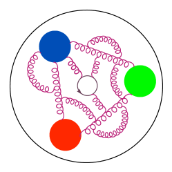
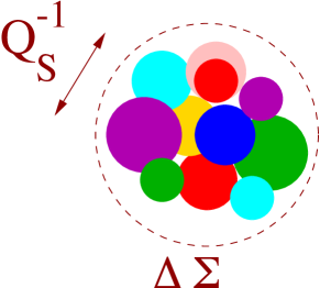
Figure 3: Left: a cartoon of the proton structure in its rest frame. Right: cartoon of one saturation disk in the infinite momentum frame (this will be discussed in sec:glasma).

The microscopic structure of a hadron depends upon the resolution scales which are used to probe it, that is, upon the kinematics of the scattering process. It furthermore depends upon the Lorentz frame in which the hadron is seen: unlike physical observables, like cross–sections, which are boost invariant, the physical interpretation of these observables in terms of partons depends upon the choice of a frame. This is best appreciated by first looking at a hadron (say, a proton) in its rest frame (RF), where the proton 4–momentum reads $P_{0}^{\mu}=(M,0,0,0)$. The proton has the quantum numbers of a system of three quarks — the ‘valence quarks’ — which are bound by confinement in a colour singlet state. But this binding proceeds via the exchange of gluons, which in turn can generate additional quark–antiquark pairs (see fig:hadron). All these partons are ‘virtual’, meaning that they keep appearing and disappearing, and have typical energies and momenta of order $\Lambda_{{\rm QCD}}$, since this is the scale where the QCD coupling becomes of $\mathcal{O}{(1)}$ and thus the binding is most efficient. Clearly, such fluctuations are non–perturbative. $\Lambda_{{\rm QCD}}$ is also the typical scale for vacuum fluctuations, like a quark–antiquark pair pumping up from the vacuum and then being reabsorbed. By the uncertainty principle, such fluctuations have lifetimes and sizes of order $1/\Lambda_{{\rm QCD}}$, of the same order as the proton size itself. Under these conditions, it makes no sense to speak about ‘hadronic substructure’ : the hadronic fluctuations are ephemeral, delocalized over the whole proton volume, and cannot be distinguished from the vacuum fluctuations having the same kinematics and quantum numbers.

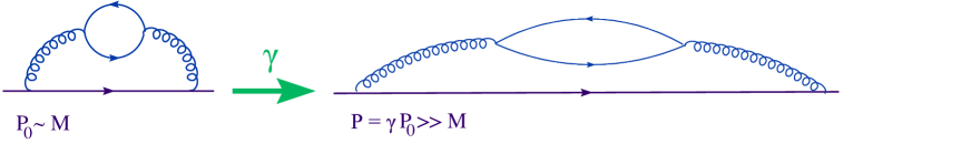
Figure 4: A hadronic fluctuation in the hadron rest frame (left) and in the infinite momentum frame (right).

However, the situation changes if one observes the same hadron in a frame which is boosted by a large Lorentz factor $\gamma\gg 1$ w.r.t. the rest frame. Then the hadron 4–momentum reads $P^{\mu}=(E,0,0,P)$ with $E=\sqrt{P^{2}+M^{2}}\simeq P$. (We have chosen the boost along the $z$ axis and denoted $P_{z}=P$.) In this boosted frame, conventionally referred to as the infinite momentum frame (IMF), the lifetime of the hadronic fluctuations is enhanced by Lorentz time dilation (see fig:boost),

$$\Delta t_{\rm IMF}\,=\,\gamma\Delta t_{\rm RF}\,\sim\,\frac{\gamma}{\Lambda_{{\rm QCD}}}\,,$$ (2)

so these fluctuations are now well separated from the those of the vacuum (which have a lifetime $\sim 1/\Lambda_{{\rm QCD}}$ in any frame, since the vacuum is boost invariant). The lifetime lifeIMF is much larger than the duration of a typical collision process (see below); so, for the purpose of scattering, the hadronic fluctuations can be viewed as free, independent quanta. These quanta are the partons (a term coined by Feynman). It then becomes possible to factorize the cross–section (say, for a hadron–hadron collision) into the product of parton distribution functions (one for each hadron partaking in the collision), which describe the probability to find a parton with a given kinematics inside the hadronic wavefunction, and partonic cross–sections, which, as their name indicates, describe the collision between subsets of partons from the target and the projectile, respectively. If the momentum transferred in the collision is hard enough, the partonic cross–sections are computable in perturbation theory. The parton distributions are a priori non–perturbative, as they encode the information about the binding of the partons within the hadron. Yet, there is much that can be said about them within perturbation theory, as we shall explain. To that aim, one needs to better appreciate the role played by the resolution of a scattering process. In turn, this can be best explained on the example of a simpler process: the electron–proton deep inelastic scattering (DIS).

  

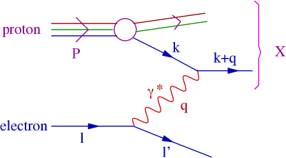
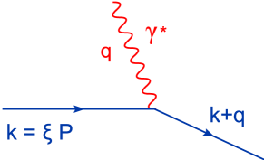
Figure 5: Left: the DIS process. Right: the absorption of the virtual photon by a quark.

The DIS process is illustrated in fig:DIS (left): an electron with 4–momentum $\ell_{\mu}$ scatters off the proton by exchanging a virtual photon ($\gamma^{*}$) with 4–momentum $q_{\mu}$ and emerges after scattering with 4–momentum $\ell^{{}^{\prime}}_{\mu}=\ell_{\mu}-q_{\mu}$. The exchanged photon is space–like :

$$q^{2}=(\ell-\ell^{\prime})^{2}=-2\ell\cdot\ell^{\prime}=-2E_{\ell}E_{\ell^{\prime}}(1-\cos\theta_{\ell\ell^{\prime}})\,\equiv\,-Q^{2}\qquad\mbox{with}\quad Q^{2}>0,$$ (3)

with $E_{\ell}=|\bm{\ell}|$, $E_{\ell^{\prime}}=|\bm{\ell}^{\prime}|$, and $\theta_{\ell\ell^{\prime}}=\angle(\bm{\ell},\bm{\ell}^{\prime})$. The positive quantity $Q^{2}$ is referred to as the ‘virtuality’. The deeply inelastic regime corresponds to $Q^{2}\gg M^{2}$, since in that case the proton is generally broken by the scattering and its remnants emerge as a collection of other hadrons (denoted by $X$ in fig:DIS). The (inclusive) DIS cross–section involves the sum over all the possible proton final states $X$ for a given $\ell^{\prime}$.

A space–like probe is very useful since it is well localized in space and time and thus provides a snapshot of the hadron substructure on controlled, transverse and longitudinal, scales, as fixed by the kinematics. Specifically, we shall argue that, when the scattering is analyzed in the proton IMF, the virtual photon measures partons which are localized in the transverse plane within an area $\Sigma\sim 1/Q^{2}$ and which carry a longitudinal momentum $k_{z}=xP$, where $x$ is the Bjorken variable :

$$x\,\equiv\,\frac{Q^{2}}{2(P\cdot q)}\,=\,\frac{Q^{2}}{s+Q^{2}-M^{2}}\,,$$ (4)

where $s\equiv(P+q)^{2}$ is the invariant energy squared of the photon+proton system. That is, the two kinematical invariants $Q^{2}$ and $x$, which are fixed by the kinematics of the initial state ($\ell,\,P$) and of the scattered electron ($\ell^{\prime}$), completely determine the transverse size ($\sim 1/Q$) and the longitudinal momentum fraction ($x$) of the parton that was involved in the scattering. This parton is necessarily a quark (or antiquark), since the photon does not couple directly to gluons. But the DIS cross–section allows us to indirectly deduce also the gluon distribution, as we shall see.

As a first step in our argument, consider a quark excitation of the hadron, viewed in the IMF. This quark is a virtual fluctuation which has been boosted together with the proton, so its virtuality and its transverse momentum are both small as compared to its longitudinal momentum $k_{z}=\xi P$. (We temporarily denote with $\xi$ the fraction of the proton longitudinal momentum which is carried by the quark.) So, for most purposes, one can treat the quark as a nearly on–shell excitation with 4–momentum as $k^{\mu}\simeq\xi P^{\mu}=(\xi P,0,0,\xi P)$ and $k^{2}\equiv k_{\mu}k^{\mu}\simeq 0$. (More precisely, $k^{2}\simeq k_{\perp}^{2}\sim\Lambda_{{\rm QCD}}^{2}$.) Such an excitation has a relatively large lifetime, which can be estimated as in lifeIMF :

$$\Delta t_{\rm fluct}\,=\,\gamma\Delta t_{\rm RF}\,\simeq\,\frac{2k_{z}}{k_{\perp}^{2}}\,=\,\frac{2\xi P}{k_{\perp}^{2}}\,,$$ (5)

where $\Delta t_{\rm RF}\sim 2/k_{\perp}$ is the lifetime of the fluctuation in the hadron rest frame and $\gamma=k_{z}/k_{\perp}$ is the boost factor from the RF to the IMF.

Consider now the absorption of the virtual photon by the quark, cf. fig:DIS right. The quark is liberated by this collision, meaning that it is put on shell; so we can write

$$(k+q)^{2}\,=\,0\,\Longrightarrow\,-Q^{2}+2\xi P\cdot q\,=\,0\,\Longrightarrow\,\xi\,=\,\frac{Q^{2}}{2(P\cdot q)}\,=\,x\,,$$ (6)

where we have also used $k^{2}\approx 0$, as discussed before. We see that the collision identifies the longitudinal momentum fraction $\xi$ of the participating quark with the Bjorken–$x$ kinematical variable, as anticipated. From now on, we shall use the notation $x$ for both quantities.

To also clarify the transverse resolution of the virtual photon, we first need an estimate for the collision time. This is the typical duration of the partonic process $q+\gamma^{*}\to q$ (cf. fig:DIS right) and is given by the uncertainty principle: $\Delta t_{\rm coll}\sim 1/\Delta E$, where $\Delta E=q_{0}+|\bm{k}+\bm{q}|-|\bm{k}|$ is the energy difference at the photon emission vertex. To estimate $\Delta E$, it is convenient to choose a space–like photon with zero energy and only transverse momentum: $q^{\mu}=(0,\bm{q}_{\perp},0)$. Then

$$\Delta E=|\bm{k}+\bm{q}|-|\bm{k}|=\sqrt{(xP)^{2}+q_{\perp}^{2}}-xP\simeq\,\frac{q_{\perp}^{2}}{2xP}\quad\Longrightarrow\quad\Delta t_{\rm coll}\simeq\frac{2xP}{Q^{2}}.$$ (7)

(Note that $Q^{2}=q_{\perp}^{2}$ for the virtual photon at hand.) In order to be ‘found’ by the photon, a quark excitation must have a lifetime larger than this collision time:

$$\Delta t_{\rm fluct}\,\simeq\,\frac{2xP}{k_{\perp}^{2}}\,>\,\Delta t_{\rm coll}\simeq\frac{2xP}{Q^{2}}\,\Longrightarrow\,k_{\perp}^{2}\,<\,Q^{2}\,.$$ (8)

Hence, the virtual photon can discriminate only those partons having transverse momenta smaller than its virtuality $Q$. By the uncertainty principle, such partons are localized within a transverse area $\sim 1/Q^{2}$, as anticipated after bj.

The previous considerations motivate the following formula for the DIS cross–section :

$$\sigma_{\gamma^{*}p}(x,Q^{2})\,=\,\frac{4\pi^{2}\alpha_{\rm em}}{Q^{2}}\,F_{2}(x,Q^{2})\,,$$ (9)

where the first factor in the r.h.s. is the elementary cross–section for the photon absorbtion by a quark (or an antiquark), whereas the second factor — the structure function $F_{2}(x,Q^{2})$ — is the sum of the quark and antiquark distribution functions, weighted by the respective electric charges squared

$$F_{2}(x,Q^{2}) \,=\,\sum_{f}e_{f}^{2}\,\big{[}xq_{f}(x,Q^{2})+x\bar{q}_{f}(x,Q^{2})\big{]}\,,$$

$$q_{f}(x,Q^{2}) \,\equiv\,\frac{\rmd N_{f}}{\rmd x}(Q^{2})\,=\,\int^{Q}\!\rmd^{2}\bm{k}_{\perp}\,\frac{\rmd N_{f}}{\rmd x\rmd^{2}\bm{k}_{\perp}}\,.$$ (10)

That is, $q_{f}(x,Q^{2})\rmd x$ is the number of quarks of flavor $f$ with longitudinal momentum fraction between $x$ and $x+\rmd x$ and which occupy a transverse area $1/Q^{2}$.

One may naively think that the condition $k_{\perp}^{2}<Q^{2}$ is trivially satisfied, since the partons confined inside the hadron have transverse momenta $k_{\perp}\sim\Lambda_{{\rm QCD}}$, whereas $Q^{2}\gg\Lambda_{{\rm QCD}}^{2}$ by the definition of DIS. If that were the case, the structure function $F_{2}(x,Q^{2})$ would be independent of $Q^{2}$ — a property known as Bjorken scaling. However, the DIS data show that Bjorken scaling holds only approximately and only in a limited range of values for $x$, namely for $x\gtrsim 0.1$. This can be understood as follows : the typical transverse momenta are $\sim\Lambda_{{\rm QCD}}$ only for the valence quarks and, more generally, for the partons with relatively large longitudinal momentum fractions. But virtual quanta with much larger values for $k_{\perp}$ can be generated via radiative processes like bremsstrahlung. Such quanta have very short lifetimes, but so long as $k_{\perp}^{2}<Q^{2}$, they can still contribute to DIS. Also, they generally have small values of $x$, as they share all together the longitudinal momenta of their parents partons. Hence, we expect the parton evolution via bremsstrahlung to lead to an increase in the parton distributions at large values of $k_{\perp}$ and small values of $x$. This evolution is responsible for the violations of the Bjorken scaling seen in the data and, more generally, for the DGLAP evolution [1, 2] of the parton distribution functions with increasing $Q^{2}$. It is furthermore responsible for the rapid growth in the gluon distribution with decreasing $x$ and the formation of a colour glass condensate at high energy. This will be further discussed in sec:evol.

3.2 Particle production at the LHC: why small $x$ ?

Before we turn to a discussion of parton evolution, let us explain here why we shall be mostly interested in partons with small longitudinal momentum fractions $x\ll 1$. As it should be clear from bj, small values of $x$ correspond to the high–energy regime at $s\gg Q^{2}$. The conceptual importance of this regime will be explained later, but for the time being let us discuss it from the experimental point of view. Very small values of $x$, as low as $x=10^{-5}\div 10^{-4}$, have been already reached in the e+p collisions at HERA, but in that context they were associated (because of the experimental constraints) with rather small values of the transferred momentum $Q^{2}$. Namely, the HERA data at $x\leq 10^{-4}$ correspond to values $Q^{2}<1$ GeV² which are only marginally under control in perturbation theory. Because of that, the DIS data at HERA remained inconclusive for a check of our theoretical understanding of the physics at small $x$.

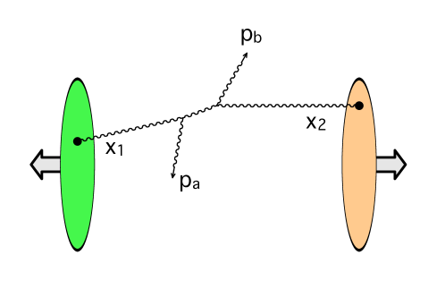
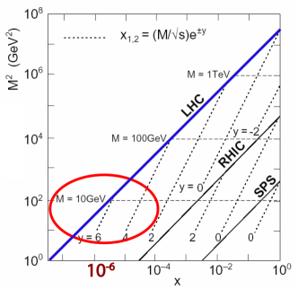
Figure 6: Left: two particle production in hadron–hadron collision. Right: the kinematical domain accessible at the LHC, as compared to RHIC and the SPS; the small–$x$ region is highlighted.

But the situation has changed with the advent of the new hadron–hadron colliders, RHIC and, especially, the LHC. Given the much higher available energies, the bulk of the particle production (with semi–hard transverse momenta) in these experiments is controlled by partons with $x\leq 10^{-3}$. Moreover, for special kinematical conditions to be shortly specified, one can probe values as low as $x\sim 10^{-6}$ with truly hard momentum transferts, such as $Q^{2}=10$ GeV².

To describe the kinematics of particle production, it is useful to introduce a new kinematical variable, the rapidity $y$, which is an alternative for the longitudinal momentum. For an on–shell particle with 4–momentum $p^{\mu}=(E,\bm{p}_{\perp},p_{z})$, the rapidity is defined as

$$y\,\equiv\,\frac{1}{2}\,\ln\frac{E+p_{z}}{E-p_{z}}\,\Longrightarrow\,E=m_{\perp}\cosh y,\quad p_{z}=m_{\perp}\sinh y\,,$$ (11)

where $m_{\perp}\equiv\sqrt{m^{2}+p^{2}_{\perp}}$ is the ‘transverse mass’ and $E^{2}=m^{2}_{\perp}+p_{z}^{2}$. Note that $y$ is positive for a ‘right–mover’ ($p_{z}>0$) and negative for a ‘left–mover’ ($p_{z}<0$). In fact, one has $v_{z}=p_{z}/E=\tanh y$, so $y$ is simply related to the longitudinal boost factor: $\gamma=\cosh y$. A similar quantity which is perhaps more useful in the experiments (since easier to measure) is the pseudo–rapidity

$$\eta\,\equiv\,\frac{1}{2}\,\ln\frac{p+p_{z}}{p-p_{z}}\,=\,-\ln\,\tan\frac{\theta}{2}\,,$$ (12)

where $p=|\bm{p}|$ is the magnitude of the 3–momentum vector. As shown by the second equality above, $\eta$ is directly related to the polar angle $\theta$ made by the particle with the longitudinal axis ($\cos\theta={p_{z}}/{p}$). For massless particles or for ultrarelativistic ones (whose masses can generally be ignored), the two rapidities coincide with each other, as manifest by comparing Eqs. ydef and etadef.

Consider now the process illustrated in fig:2part (left), i.e. the production of a pair of particles in a partonic subcollision of a hadron–hadron scattering. In the center–of–mass (COM) frame, the two partons partaking in the collision have 4–momenta $k_{i}^{\mu}=x_{i}P_{i}^{\mu}+k^{\mu}_{i\perp}$ where $i=1,2$, $P_{1}^{\mu}=(P,0,0,P)$, $P_{2}^{\mu}=(P,0,0,-P)$, and $k^{\mu}_{i\perp}=(0,\bm{k}_{i\perp},0)$. Notice that $P=\sqrt{s}/2$. The two outgoing particles will be characterized by the respective transverse momenta, $\bm{p}_{a\perp}$ and $\bm{p}_{b\perp}$, and rapidities, $y_{a}$ and $y_{b}$. Energy–momentum conservation implies $\bm{p}_{a\perp}+\bm{p}_{b\perp}=\bm{k}_{1\perp}+\bm{k}_{2\perp}$ and

$$x_{1}\,=\,\frac{p_{a\perp}}{\sqrt{s}}\,\rme^{y_{a}}+\frac{p_{b\perp}}{\sqrt{s}}\,\rme^{y_{b}}\,,\qquad x_{2}\,=\,\frac{p_{a\perp}}{\sqrt{s}}\,\rme^{-y_{a}}+\frac{p_{b\perp}}{\sqrt{s}}\,\rme^{-y_{b}}\,.$$ (13)

For particle production at RHIC or the LHC, the average transverse momentum of a hadron in the final state is below 1 GeV ; moreover, 99% of the ‘multiplicity’ (i.e. of the total number of produced hadrons) has $p_{\perp}\leq 2$ GeV (see fig:avept). For $p_{a,b\,\perp}=1$ GeV and central rapidities $y_{a,b}\simeq 0$, 2pkin implies

$$x_{i}\simeq 10^{-2}\ \mbox{at RHIC}\ (\sqrt{s}=200\,\mbox{GeV}),\qquad\quad x_{i}\simeq 4\times 10^{-4}\ \mbox{at the LHC}\ (\sqrt{s}=2.76\,\mbox{TeV}),$$ (14)

where in the case of the LHC we have chosen the maximal COM energy per nucleon pair that has been reached so far in Pb+Pb collisions. Thus, the bulk of the particle production is initiated by partons carrying small values of $x$, as anticipated. Moreover, one of these values ($x_{1}$ or $x_{2}$) can be made much smaller by studying particle production at either forward, or backward, rapidities. The rapidities are ‘forward’ when both $y_{a}$ and $y_{b}$ are positive and relatively large, that is, the final particles propagate essentially along the same direction as the original hadron ‘1’ ; then their production probes very small values of $x_{2}$ in the wavefunction of the hadron ‘2’ and comparatively large values of $x_{1}$. At the LHC, one can probe values as small as $x_{2}\sim 10^{-6}$ for $p_{\perp}\sim 10$ GeV, as indicated in the r.h.s. of fig:2part.

   

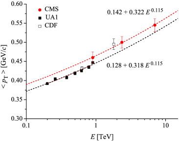
Figure 7: Transverse momentum dependence of the single inclusive particle production in hadron–hadron collisions. Left: Pb+Pb collisions at the LHC. Right: p+p collisions at the LHC and p+$\overline{\mbox{p}}$ collisions at SPS and CDF.

We finally discuss the cross–section for the production of a pair of hadrons. When the transverse momenta $p_{a,b\,\perp}$ are large enough, one can ignore the ‘intrinsic’ transverse momenta $\bm{k}_{1,2\,\perp}$ of the colliding partons. Then the transverse momentum conservation $\bm{p}_{a\perp}+\bm{p}_{b\perp}\simeq 0$ implies that the outgoing particles propagate back–to–back in the transverse plane, i.e. they make an azimuthal angle $\Delta\phi\simeq\pi$. The associated cross–section admits the following collinear factorization, analogous to F2 for DIS

$$\frac{\rmd\sigma}{\rmd p_{\perp}^{2}\rmd y_{1}\rmd y_{2}}=\sum_{ij}x_{1}f_{i}(x_{1},\mu^{2})\,x_{2}f_{j}(x_{2},\mu^{2})\,\frac{\rmd\hat{\sigma}_{ij}}{\rmd p^{2}_{\perp}}\,,$$ (15)

where $xf_{i}(x,\mu^{2})$ are parton distributions for all species of partons ($i=q,\bar{q},g$), $\mu^{2}$ is the factorization scale, and ${\rmd\hat{\sigma}_{ij}}/{\rmd p^{2}_{\perp}}$ is the cross–section for the (relatively hard) partonic process $i+j\to a+b$. Leading–order perturbative QCD yields ${\rmd\hat{\sigma}}/{\rmd p^{2}_{\perp}}\propto\alpha_{s}^{2}/p^{4}_{\perp}$ at high energy. So, if one tries to compute the total multiplicity by integrating over all values of $p_{\perp}^{2}$ (say, for $y_{a}\sim y_{b}\sim 0$), then one faces a quadratic infrared divergence from the limit $p_{\perp}^{2}\to 0$. One may think that this divergence is cut off at $p_{\perp}\sim\Lambda_{{\rm QCD}}$, since this is the typical value expected for the intrinsic momenta $k_{1,2\,\perp}$. But then one would conclude that the bulk of the particle production, even at very high energy, is concentrated at very soft transverse momenta, of the order of the confinement scale $\Lambda_{{\rm QCD}}$. Moreover, the average $p_{\perp}$ would be independent of the energy (since of $\mathcal{O}{(\Lambda_{{\rm QCD}})}$). These conclusions are however contradicted by the data in fig:avept, which rather show that $\langle p_{\perp}\rangle\simeq 0.5$ GeV is about 2 to 3 times larger than $\Lambda_{{\rm QCD}}$ at the LHC energies and, remarkably, it clearly rises with the COM energy $E=\sqrt{s}$. This conflict between the data and the prediction coll of collinear factorization clearly shows that the latter cannot be extrapolated down to lower values for $p_{\perp}$, say of order 1 GeV. The proper way to describe this semi–hard region within (perturbative) QCD will be explained in the next subsection. The main outcome of that analysis will be to introduce a new infrared cutoff in the problem, which is dynamically generated — via gluon evolution with decreasing $x$ — and rises as a power of the energy. This is the saturation momentum.

3.3 Gluon evolution at small $x$

In perturbative QCD, parton evolution proceeds via bremsstrahlung, which favors the emission of soft and collinear gluons, i.e. gluons which carry only a small longitudinal momentum fraction $x\ll 1$ and a relatively small transverse momentum $k_{\perp}$. onegluon illustrates one elementary step in this evolution: the emission of a gluon which carries a fraction $x=k_{z}/p_{z}$ of the longitudinal momentum of its parent parton (quark or gluon). For $x\ll 1$ and to lowest order in $\alpha_{s}$, the differential probability for this emission (obtained as the modulus squared of the amplitude represented in onegluon) reads

$$\rmd P_{\rm Brem}\,\simeq\,C_{R}\frac{\alpha_{s}(k_{\perp}^{2})}{\pi^{2}}\,\frac{\rmd^{2}k_{\perp}}{k_{\perp}^{2}}\,\frac{\rmd x}{x}\;,$$ (16)

where $C_{R}$ is the SU$(N_{c})$ Casimir in the colour representation of the emitter: $C_{A}=N_{c}$ for a gluon and $C_{F}=(N_{c}^{2}-1)/2N_{c}$ for a quark. ($N_{c}$ is the number of colours, which is equal to 3 in real QCD, but it is often kept as a free parameter in theoretical studies, because many calculations simplify in the formal limit $N_{c}\gg 1$. The results obtained in this limit provide insightful, qualitative and semi–quantitative informations about real QCD.) brem exhibits the collinear ($k_{\perp}\to 0$) and soft ($x\to 0$) singularities mentioned above, which result in the enhancement of gluon emission at small $k_{\perp}$ and/or $x$. If the emitted parton with small $x$ were a quark instead a gluon, there would be no small $x$ enhancement, only the collinear one. This asymmetry, due to the spin–1 nature of the gluon, has the remarkable consequence that the small–$x$ part of the wavefunction of any hadron is built mostly with gluons.

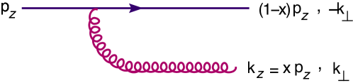
Figure 8: Gluon bremsstrahlung out of a parent quark to lowest order in pQCD.

As manifest on brem, parton branching is suppressed by a power of $\alpha_{s}(k_{\perp}^{2})$, which is small when $k_{\perp}\gg\Lambda_{{\rm QCD}}$. But this suppression can be compensated by the large phase–space available for the emission, which equals $\ln(Q^{2}/\Lambda_{{\rm QCD}}^{2})$ for the emission of a parton (quark or gluon) with transverse momentum $k_{\perp}\ll Q$ and, respectively, $\ln(1/x)$ for that of a gluon with longitudinal momentum fraction $\xi$ within the range $x\ll\xi\ll 1$. Hence, for large $Q^{2}\gg\Lambda_{{\rm QCD}}^{2}$ and/or small $x\ll 1$, such radiative processes are not suppressed anymore and must be resummed to all orders. Depending upon the relevant values of $Q^{2}$ and $x$, one can write down evolution equations which resum either powers of $\alpha_{s}\ln(Q^{2}/\Lambda_{{\rm QCD}}^{2})$, or of $\alpha_{s}\ln(1/x)$, to all orders. The coefficients in these equations represent the elementary splitting probability and can be computed as power series in $\alpha_{s}$, starting with the leading–order result in Eq. (16).

The evolution with increasing $Q^{2}$ is described by the DGLAP equation (from Dokshitzer, Gribov, Lipatov, Altarelli and Parisi) [1, 2]. This evolution mixes quarks and gluons (see Fig. 9.a), which in particular allows us to reconstruct the gluon distribution from the experimental results for $F_{2}$. The small–$x$ evolution, on the other hand, involves only gluons and corresponds to resumming ladder diagrams like those in Fig. 9.b in which successive gluons are strongly ordered in $x$ (see below). Both evolutions lead to an increase in the number of partons at small values of $x$ (and a decrease at large values $x\gtrsim 0.1$), but the physical consequences are very different in the two cases:

(i) When increasing $Q^{2}$, one emits partons which occupy a smaller transverse area $\sim 1/Q^{2}$, as shown in HERA-gluon (right). The decrease in the area of the individual partons is much stronger than the corresponding increase in their number. Accordingly, the occupation number in the transverse plane decreases with increasing $Q^{2}$, meaning that the partonic system becomes more and more dilute. Accordingly, the partons may be viewed as independent. This observation lies at the basis of the conventional parton picture, which applies for sufficiently high $Q^{2}$ (at a given value of $x$).

The parton occupation number mentioned above yields the proper measure of the parton density in the hadron. It can be estimated as [the number of partons with a given value of $x$] $\times$ [the area occupied by one parton] divided by [the transverse area of the hadron], that is (for gluons, for definiteness),

$$n(x,Q^{2})\,\simeq\,\frac{xg(x,Q^{2})}{Q^{2}R^{2}}\,,\qquad\mbox{with}\quad g(x,Q^{2})\,\equiv\,\frac{\rmd N_{g}}{\rmd x}(Q^{2})\,=\,\int^{Q}\!\rmd^{2}\bm{k}_{\perp}\,\frac{\rmd N_{g}}{\rmd x\rmd^{2}\bm{k}_{\perp}}\,,$$ (17)

where $R$ is the hadron radius in its rest frame (so its transverse area is $\sim\pi R^{2}$ in any frame). The numerator in the above definition of the occupation number, that is

$$xg(x,Q^{2})\,\equiv\,x\,\frac{\rmd N_{g}}{\rmd x}\,=\,k_{z}\,\frac{\rmd N_{g}}{\rmd k_{z}}\,\simeq\,\frac{\Delta N_{g}}{\Delta z\,\Delta k_{z}}\,,$$ (18)

is known as the gluon distribution. The last estimate above follows from the uncertainty principle: partons with longitudinal momentum $k_{z}=xP$ are delocalized in $z$ over a distance $\Delta z\simeq 1/k_{z}$. Hence, the gluon distribution yields the number of gluons per unit of longitudinal phase–space, which is indeed the right quantity for computing the occupation number. Note that gluons with $x\ll 1$ extends in $z$ over a distance $\Delta z\sim 1/xP$ which is much larger than the Lorentz contracted width of the hadron, $R/\gamma\sim 1/P$. This shows that the image of an energetic hadron as a ‘pancake’, that would be strictly correct if the hadron was a classical object, is in reality a bit naive: it applies for the valence quarks with $x\sim\mathcal{O}{(1)}$ (which carry most of the total energy), but not also for the small–$x$ partons (which are the most numerous, as we shall shortly see).

      

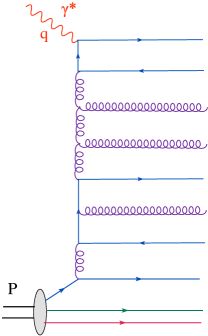
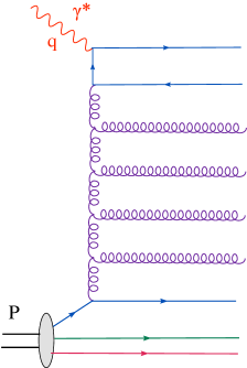
Figure 9: Parton evolution in perturbative QCD. The parton cascade on the right involves only gluons (at intermediate stages) and is a part of the BFKL resummation at small $x$ (see the discussion around eq:unintp).

(ii) When decreasing $x$ at a fixed $Q^{2}$, one emits mostly gluons which have smaller longitudinal momentum fractions, but which occupy, roughly, the same transverse area as their parent gluons (see HERA-gluon right). Then the gluon occupation number, occup, increases, showing that the gluonic system evolves towards increasing density. As we shall see, this evolution is quite fast and eventually leads to a breakdown of the picture of independent partons.

In order to describe the small–$x$ evolution, let us start with the gluon distribution generated by a single valence quark. This can be inferred from the bremsstrahlung law in brem (the emission probability is the same as the number of emitted gluons) and reads

$$x\frac{\rmd N_{g}}{\rmd x}(Q^{2})\,=\,\frac{\alpha_{s}C_{F}}{\pi}\,\int_{\Lambda_{{\rm QCD}}^{2}}^{Q^{2}}\frac{\rmd k_{\perp}^{2}}{k_{\perp}^{2}}\,=\,\frac{\alpha_{s}C_{F}}{\pi}\,\ln\left(\frac{Q^{2}}{\Lambda_{{\rm QCD}}^{2}}\right)\;,$$ (19)

where we have ignored the running of the coupling — formally, we are working to leading order (LO) in pQCD where the coupling can be treated as fixed — and the ‘infrared’ cutoff $\Lambda_{{\rm QCD}}$ has been introduced as a crude way to account for confinement: when confined inside a hadron, a parton has a minimum virtuality of $\mathcal{O}{(\Lambda_{{\rm QCD}}^{2})}$. In xGxp it is understood that $x\ll 1$. In turn, the soft gluon emitted by the valence quark can radiate an even softer gluon, which can radiate again and again, as illustrated in figure 10. Each emission is formally suppressed by a power of $\alpha_{s}$, but when the final value of $x$ is tiny, the smallness of the coupling constant can be compensated by the large available phase–space, of order $\ln(1/x)$ per gluon emission. This evolution leads to an increase in the number of gluons with $x\ll 1$.

For a quantitative estimate, consider the first such correction, that is, the two–gluon diagram in Fig. 10 left: the region in phase–space where the longitudinal momentum fraction $x_{1}$ of the intermediate gluon obeys $x\ll x_{1}\ll 1$ provides a contribution of relative order

$$\frac{\alpha_{s}N_{c}}{\pi}\,\int_{x}^{1}\frac{\rmd x_{1}}{x_{1}}\,=\,\bar{\alpha}_{s}\ln\frac{1}{x}\,,\qquad\bar{\alpha}_{s}\equiv\frac{\alpha_{s}N_{c}}{\pi}\,.$$ (20)

When $\bar{\alpha}_{s}\ln(1/x)\sim 1$, this becomes of $\mathcal{O}{(1)}$, meaning that this two–gluon diagram contributes on the same footing as the single gluon emission in Fig. 8. A similar conclusion holds for a diagram involving $n$ intermediate gluons strongly ordered in $x$, cf. Fig. 10 right, which yields a relative contribution of order

$$\bar{\alpha}_{s}^{n}\,\int_{x}^{1}\frac{\rmd x_{n}}{x_{n}}\int_{x_{n}}^{1}\frac{\rmd x_{n-1}}{x_{n-1}}\cdots\int_{x_{2}}^{1}\frac{\rmd x_{1}}{x_{1}}\,=\,\frac{1}{n!}\left(\bar{\alpha}_{s}\ln\frac{1}{x}\right)^{n}\;.$$ (21)

When $\bar{\alpha}_{s}\ln(1/x)\gtrsim 1$, the correct result for the gluon distribution at leading order is obtained by summing contributions from all such ladders. As clear from ngluons, this sum exponentiates, modifying the integrand of Eq. (19) into

$$x\frac{\rmd N_{g}}{\rmd x\rmd k_{\perp}^{2}}\,\sim\,\frac{\alpha_{s}C_{F}}{\pi}\,\frac{1}{k_{\perp}^{2}}\,\rme^{\omega\bar{\alpha}_{s}Y}\;,\qquad Y\equiv\ln\frac{1}{x}\;,$$ (22)

where $\omega$ is a number of order unity which cannot be determined via such simple arguments. The variable $Y$ is the rapidity difference between the final gluon and the original valence quark and it is often simply referred to as ‘the rapidity’. The quantity in the l.h.s. of eq:unintp is the number of gluons per unit rapidity and with a given value $k_{\perp}$ for the transverse momentum, a.k.a. the unintegrated gluon distribution.

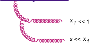
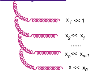
Figure 10: Gluon cascades produced by the high–energy (BFKL) evolution of the proton wavefunction.

To go beyond this simple power counting argument, one must treat more accurately the kinematics of the ladder diagrams and include the associated virtual corrections. The result is the BFKL equation (from Balitsky, Fadin, Kuraev, and Lipatov) [3] for the evolution of the unintegrated gluon distribution with $Y$. The solution of this equation, which resums perturbative corrections $(\bar{\alpha}_{s}Y)^{n}$ to all orders, confirms the exponential increase in Eq. (22), albeit with a $k_{\perp}$–dependent exponent and modifications to the $k_{\perp}^{-2}$–spectrum of the emitted gluons.

An important property of the BFKL ladder is its coherence in time : the lifetime of a parton being proportional to its value of $x$, $\Delta t\simeq 2k_{z}/k_{\perp}^{2}\propto x$, cf. lifetime, the ‘slow’ gluons at the lower end of the cascade have a much shorter lifetime than the preceding ‘fast’ gluons. Therefore, for the purposes of small–$x$ dynamics, fast gluons with $x^{\prime}\gg x$ act as frozen colour sources emitting gluons at the scale $x$. Because these sources may overlap in the transverse plane, their colour charges add coherently, giving rise to a large colour charge density. The average colour charge density is zero by gauge symmetry but fluctuations in the colour charge density — as measured in particular by the unintegrated gluon distribution — are nonzero and increase rapidly with $1/x$, cf. eq:unintp.

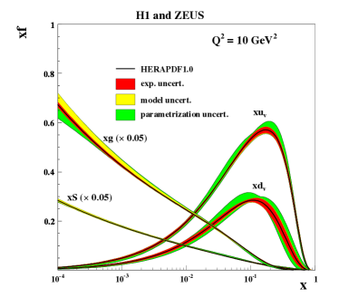
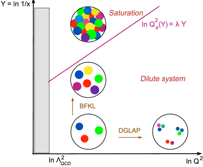
Figure 11: Left: the $1/x$–evolution of the gluon, sea quark, and valence quark distributions for $Q^{2}=10$ GeV², as measured at HERA (combined H1 and ZEUS analysis [4]). Note that the gluon and sea quark distributions have been reduced by a factor of 20 to fit inside the figure. Right: the ‘phase–diagram’ for parton evolution in QCD; each coloured blob represents a parton with transverse area $\Delta x_{\perp}\sim 1/Q^{2}$ and longitudinal momentum $k_{z}=xP$. The straight line $\ln Q_{s}^{2}(x)=\lambda Y$ is the saturation line, cf. QsxA, which separates the dense and dilute regimes.

This growth is indeed seen in the data: e.g., the HERA data for DIS confirm that the proton wavefunction at $x<0.01$ is totally dominated by gluons (see HERA-gluon left). However, on physical grounds, such a rapid increase in the gluon distribution cannot go on for ever (that is, down to arbitrarily small values of $x$). Indeed, the BFKL equation is linear — it assumes that the radiated gluons do not interact with each other, like in the conventional parton picture. While such an assumption is perfectly legitimate in the context of the $Q^{2}$–evolution, which proceeds towards increasing diluteness, it eventually breaks down in the context of the $Y$–evolution, which leads to a larger and larger gluon density. As long as the gluon occupation number occup is small, $n\ll 1$, the system is dilute and the mutual interactions of the gluons are negligible. When $n\sim\mathcal{O}{(1)}$, the gluons start overlapping, but their interactions are still weak, since suppressed by $\alpha_{s}\ll 1$. The effect of these interactions becomes of order one only when $n$ is as large as $n\sim\mathcal{O}{(1/\alpha_{s})}$. When this happens, non–linear effects (to be shortly described) become important and stop the further growth of the gluon distribution. This phenomenon is known as gluon saturation [5, 6, 7]. An important consequence of it is to introduce a new transverse–momentum scale in the problem, the saturation momentum $Q_{s}(x)$, which is determined by occup together with the condition that $n\sim{1/\alpha_{s}}$ :

$$n\big{(}x,Q^{2}=Q_{s}^{2}(x)\big{)}\,\sim\,\frac{1}{\alpha_{s}}\ \Longrightarrow\ Q_{s}^{2}(x)\,\simeq\,\alpha_{s}\frac{xg\big{(}x,Q_{s}^{2}(x)\big{)}}{R^{2}}\,.$$ (23)

Except for the factor $\alpha_{s}$, the r.h.s. of Qsat is recognized as the density of gluons per unit transverse area, for gluons localized within an area $\Sigma\sim 1/Q_{s}^{2}(x)$ set by the saturation scale. Gluons with $k_{\perp}\leq Q_{s}(x)$ are at saturation: the corresponding occupation numbers are large, $n\sim 1/\alpha_{s}$, but do not grow anymore when further decreasing $x$. Gluons with $k_{\perp}\gg Q_{s}(x)$ are still in a dilute regime: the occupation numbers are relatively small $n\ll 1/\alpha_{s}$, but rapidly increasing with $1/x$ via the BFKL evolution. The separation between the saturation (or dense, or CGC) regime and the dilute regime is provided by the saturation line in HERA-gluon right, to be further discussed below.

The microscopic interpretation of Qsat can be understood with reference to fig:Qsat (left) : gluons which have similar values of $x$ (and hence overlap in the longitudinal direction) and which occupy a same area $\sim 1/Q^{2}$ in the transverse plane can recombine with each other, with a cross–section $\sigma_{gg\to g}\simeq\alpha_{s}/Q^{2}$. After taking also this effect into account, the change in the gluon distribution in one step of the small–$x$ evolution (i.e. under a rapidity increment $Y\to Y+\rmd Y$) can be schematically written as

$$\frac{\partial}{\partial Y}\,xg(x,Q^{2})\,=\,\omega\bar{\alpha}_{s}xg(x,Q^{2})-\,\bar{\alpha}_{s}\,\frac{\alpha_{s}}{Q^{2}R^{2}}\,{\big{[}xg(x,Q^{2})\big{]}^{2}}\;.$$ (24)

The overall factor of $\bar{\alpha}_{s}$ in the r.h.s. comes from the differential probability $\propto\bar{\alpha}_{s}\rmd Y$ to emit one additional gluon in this evolution step, cf. brem. The first term, linear in $xg(x,Q^{2})$, represents the BFKL evolution; by itself, this would lead to the exponential growth with $Y$ shown in eq:unintp. The second term, quadratic in $xg(x,Q^{2})$, is the rate for recombination. This is formally suppressed by one factor $\alpha_{s}$, but it becomes as important as the first term when $Q^{2}$ is of the order of the saturation momentum $Q_{s}^{2}(x)$ introduced in Qsat. When that happens, the r.h.s. of eq:GLR vanishes, and then the gluon distribution stops growing with $Y$. The above argument, due to Gribov, Levin and Ryskin back in 1983 [5], is a bit oversimplified (and the actual evolution equation is considerably more complicated than eq:GLR; see the review papers [8, 9, 10, 11, 12, 13, 14, 15] and the discussion in sec:jimwlk below), but it has the merit to illustrate in a simple way the physical mechanism at work: the gluon occupation numbers saturate because the non–linear effects associated with the high gluon density compensate the bremsstrahlung processes.

   

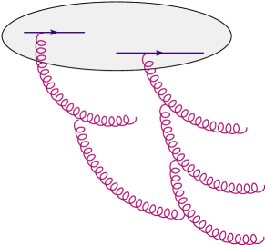
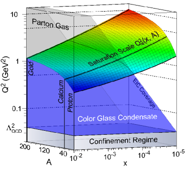
Figure 12: Left: $gg\to g$ recombination process leading to saturation. Right: the saturation momentum $Q_{s}(x,A)$ as a function of the longitudinal momentum fraction $x$ and of the atomic number $A$.

Remarkably, Qsat implies that the saturation momentum increases with $1/x$, since so does the gluon distribution for $k_{\perp}\gtrsim Q_{s}(x)$, cf. eq:unintp. So, for sufficiently small values of $x$ (say, $x\leq 10^{-4}$ in the case of a proton), one expects $Q_{s}^{2}(x)\gg\Lambda_{{\rm QCD}}^{2}$. In that case, the (semi)hard scale $Q_{s}(x)$ supplants $\Lambda_{{\rm QCD}}$ as an infrared cutoff for the calculation of physical observables like the multiplicity (cf. the discussion at the end of sec:eta). This has the remarkable consequence that, for sufficiently high energy, the bulk of the particle production can be computed in perturbation theory. But the proper framework to perform this calculation is not standard pQCD as based on the collinear factorization, but the CGC effective theory which includes the non–linear physics of gluon saturation. This will be discussed in the next subsection.

Gluon occupancy is further amplified if instead of a proton we consider a large nucleus with atomic number $A\gg 1$. The corresponding gluon distribution $xg_{A}(x,Q^{2})$ scales like $A$, since gluons can be radiated by any of the $3A$ valence quarks of the $A$ nucleons. Since the nuclear radius scales like $R_{A}\sim A^{1/3}$, occup implies that the gluon occupation number scales as $A^{1/3}$. This factor is about 6 for the Au and Pb nuclei respectively used at RHIC and the LHC. Thus, for a large nucleus, saturation effects become important at larger values of $x$ than for a proton. This explains why ultrarelativistic heavy ion collisions represent a privileged playground for observing and studying the effects of saturation.

fig:Qsat (right) summarizes our current expectations for the value and the variation of the saturation momentum. The dependence upon $x$ is by now known to next-to-leading-order (NLO) accuracy [16] — that is, by resumming radiative corrections $\alpha_{s}\big{[}\alpha_{s}\ln(1/x)\big{]}^{n}$ to all orders together with non–linear effects. The result can be roughly expressed as

$$Q^{2}_{s}(x,A)\,\simeq\,Q_{0}^{2}\,A^{1/3}\left(\frac{x_{0}}{x}\right)^{\lambda}\,,\qquad\mbox{with}\quad\lambda=0.2\div 0.3\,,$$ (25)

with the power $\lambda$ known as the saturation exponent. The overall scale $Q_{0}^{2}$, which has the meaning of the proton saturation scale at the original value $x_{0}$, is non–perturbative and cannot be computed within the CGC effective theory. (The latter governs only the evolution from $x_{0}$ down to $x\ll x_{0}$.) In practice, this is treated as a free parameter which is fitted from the data. The fits yield $Q_{0}\simeq 0.5$ GeV for $x_{0}=10^{-2}$. fig:Qsat shows that for $x=10^{-5}$ (a typical value for forward particle production at the LHC), $Q_{s}\simeq 1$ GeV for the proton, while $Q_{s}\simeq 3$ GeV for the Pb nucleus. This difference is significant: while 1 GeV is only marginally perturbative, 3 GeV is sufficiently ‘hard’ to allow for controlled perturbative calculations. This confirms the usefulness of HIC as a laboratory to study saturation.

   

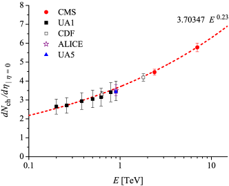
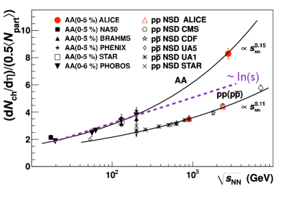
Figure 13: Charged particles multiplicity at central (pseudo)rapidity $\eta=0$ as a function of the COM energy for p+p and nucleus–nucleus collisions. The data are consistent with a power–law increase with $\sqrt{s}$ (with an exponent which is slightly larger for A+A than for p+p), but appear to exclude a logarithmic law $\propto\ln s$.

Before we conclude this subsection, let us notice some robust predictions of the saturation physics, which do not require a detailed theory and can be directly checked against the data. One of them refers to the energy–dependence of the average transverse momentum of the produced particles: as shown in fig:avept, this grows like a power of $E=\sqrt{s}$, with an exponent which is fitted from the data as $0.115$. This is consistent with expectations based on gluon saturation [17]. Indeed, prior to the collision, the gluon distribution inside the hadron wavefunction is peaked at $k_{\perp}\sim Q_{s}$ (see fig:Phi below and the related discussion) and these gluons are then released in the final state. We thus expect the average $p_{\perp}$ of the produced hadrons to scale like $Q_{s}(x)$ evaluated at the appropriate value of $x$, that is, $x=p_{\perp}/E$ (cf. 2pkin). This argument implies $\langle p_{\perp}\rangle\propto E^{\lambda/2}$, which is indeed consistent with the data in fig:avept (right) together with the estimate in QsxA for the saturation exponent. Another prediction of this kind refers to the particle multiplicity in the final state $\rmd N/\rmd\eta$, say, at central (pseudo)rapidity $\eta=0$. By the above argument, this is dominated by gluons with $Q^{2}\simeq Q_{s}^{2}(x)$ and hence it is proportional to the respective gluon distribution, that is, to $Q_{s}^{2}(x)$ itself (cf. Qsat) : $\rmd N/\rmd\eta\,\propto\,Q_{s}^{2}(E)\sim E^{\lambda}$. Once again, this appears to be consistent with the data for both p+p and A+A collisions, as shown in fig:multiplicity.

3.4 The CGC effective theory

The partonic form of matter made with the saturated gluons is known as the colour glass condensate [8, 9, 10, 11, 12, 13, 14, 15].

• This is coloured since gluons carry the ‘colour’ charge of the non–Abelian group SU$(3)$.

• It is a glass because of the separation in time scales, due to Lorentz time dilation, between the ‘slow’ gluons at small $x$ and their ‘fast’ sources at larger $x$. The sources appear as ‘frozen’ over the characteristic time scales for the dynamics at small $x$, but they can vary over much larger time scales, as set by their own, comparatively large, longitudinal momenta. A system which behaves as a solid on short time scales and as a fluid on much longer ones, is a glass.

• It is a condensate because the saturated gluons and their sources have high occupation numbers $n(x,k_{\perp})\sim 1/\alpha_{s}$ and their colour charges add coherently to each other, as explained in sec:evol in relation with the BFKL ladder. A coherent quantum state with high occupancy can be in a first approximation described as a classical field (here, a colour field), which is the most generic example of a condensate.

Because of its high density, the CGC is weakly coupled and thus it can be studied within perturbative QCD. This is strictly correct for sufficiently small values of $x$, such that $Q_{s}^{2}(x)\gg\Lambda_{{\rm QCD}}^{2}$ and hence $\alpha_{s}(Q_{s}^{2})\ll 1$, but it remains marginally true for the phenomenology at RHIC and, especially, the LHC, where the saturation momentum is semi–hard, cf. fig:Qsat (right). Based on that, an effective theory has been explicitly constructed, which resums an infinite series of Feynman graphs of the ordinary perturbation theory — those which are enhanced by either the large logarithm $\ln(1/x)$, or by the high gluon density. This theory governs the dynamics of the gluons with a given, small, value of $x$, while the gluons at larger values $x^{\prime}\gg x$ have been ‘integrated out’ in perturbation theory. In order to describe its mathematical structure, it is useful to recall that the gluon field in QCD is represented by a non–Abelian vector potential $A^{\mu}_{a}(x)$ where the upper index $\mu$ refers to the 4 Minkowski coordinates and the subscript $a$ is a colour index in the adjoint representation of SU$(N_{c})$ and can take $N_{c}^{2}-1=8$ values.

The CGC effective theory may be viewed as a non–linear generalization of the BFKL evolution, but in fact it is much more complex than just a non–linear evolution equation (say, like that in eq:GLR). The BFKL equation applies to the unintegrated gluon distribution (or occupation number), which is a Fourier transform of the 2–point function $\langle A^{i}_{a}(x)A^{i}_{a}(y)\rangle$ of the colour fields within the hadron (The average refers to the hadron wavefunction and the upper index $i$ with $i=1,2$ indicates the transverse directions.) This quantity offers more information than the standard parton distributions like $xg(x,Q^{2})$ — it also describes the distribution of gluons in transverse momentum, and not only in $x$ —, but it still does not probe many–body correlations in the gluon distribution, as the higher $n$–point functions with $n\geq 4$ would do. The restriction to the 2–point function is justified so long as the system is dilute and gluons do not interact with each other. But this cannot encode the non–linear physics of saturation, which is sensitive to higher $n$–point functions and hence to correlations. In fact, to correctly describe gluon saturation, one needs to control $n$–point functions with arbitrarily high $n$. This can be understood as follows: the fact that the occupation numbers are $n\sim\mathcal{O}{(1/\alpha_{s})}$ at saturation, means that the colour field strengths are as large as $A^{i}_{a}\sim\mathcal{O}{(1/g)}$, and then there is no penalty for inserting arbitrary powers of $A^{i}_{a}$. Indeed, any such an insertion is accompanied by a factor of $g$. (Recall that interactions in QCD enter via the covariant derivative $D^{\mu}=\partial^{\mu}-igA^{\mu}$.) So, the CGC effective theory is truly an infinite hierarchy of coupled evolution equations describing the simultaneous evolution of all the $n$–point functions. Remarkably enough, this hierarchy can be summarized into a single, functional, evolution equation for the CGC weight function — a functional generalization of the ‘unintegrated’ gluon distribution that will be shortly discussed.

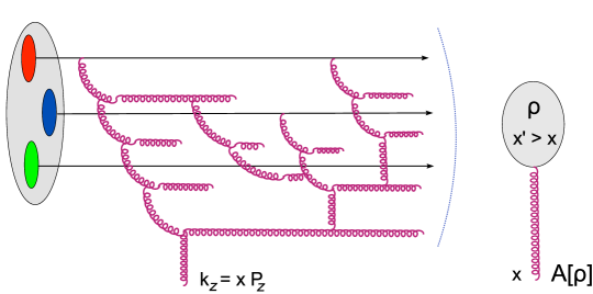
Figure 14: Schematic representation of the d.o.f. involved in the CGC effective theory and of the quantum evolution which is taken into account in this theory. A newly emitted gluon with a small longitudinal momentum fraction $x\ll 1$ rescatter off the gluon field $A^{\mu}_{a}[\rho]$ created in the previous steps by the gluons with larger values $x^{\prime}\gg x$, effectively represented by their global colour charge density $\rho_{a}$.

The key ingredient for such an economical description is the proper choice of the relevant degrees of freedom: as already mentioned, the small–$x$ gluons with high occupation numbers $n\sim 1/\alpha_{s}$ can be treated semi–classically to leading order in $\alpha_{s}$ — that is, they can be described as classical colour fields $A^{\mu}_{a}(x)$ radiated by colour sources representing the faster gluons with $x^{\prime}\gg x$. This distinction between ‘classical fields’ (= the small–$x$ gluons for which the effective theory is built) and their ‘sources’ (= the large–$x$ gluons which are integrated out in the construction of the effective theory) is illustrated in fig:CGC. The effective theory based on this separation is valid to LO in $\alpha_{s}$, but to all orders in $\alpha_{s}\ln(1/x)$ and in the classical field $A^{\mu}_{a}\sim\mathcal{O}{(1/g)}$.

The mathematical structure of the CGC theory is rather complex and it will be only schematically described here. To that aim, it is convenient to switch to light–cone vector notations. Namely, for any 4–vector such as $x^{\mu}$, $p^{\mu}$, $A^{\mu}_{a}$ etc. we shall define its light–cone (LC) components as

$$x^{+}\equiv\frac{1}{\sqrt{2}}\,(x^{0}+x^{3})\,,\quad x^{-}\equiv\frac{1}{\sqrt{2}}\,(x^{0}-x^{3})\,,\quad x^{\mu}_{\rm LC}=(x^{+},x^{-},\bm{x}_{\perp})\,.$$ (26)

In LC notations, the scalar product reads $k\cdot x\equiv k_{\mu}x^{\mu}=k^{+}x^{-}+k^{-}x^{+}-\bm{k}_{\perp}\cdot\bm{x}_{\perp}$.

To see the usefulness of these notations, consider a right–moving ultrarelativistic hadron, with $P^{\mu}\simeq(P,0,0,P)$ : this propagates at nearly the speed of light along the trajectory $x^{3}=t$. In LC notations, the 4–momentum $P^{\mu}_{\rm LC}\simeq(\sqrt{2}P,0,0,0)$ has only a ‘plus’ component, while the trajectory reads simply $x^{-}=0$. The same holds for any of the large–$x$ partons which move quasi–collinearly with the hadron and serve as sources for the small–$x$ gluons that we are interested in. In the semi–classical approximation, these small–$x$ gluons are described as the solution to the Yang–Mills equations (the non–Abelian generalization of the Maxwell equations) having these ‘fast’ gluons as sources:

$$D_{\nu}^{ab}F_{b}^{\nu\mu}(x)\,=\,\delta^{\mu+}\rho^{a}(x^{-},\bm{x}_{\perp})\,.$$ (27)

In this equation, the l.h.s. features the covariant derivative $D_{\nu}^{ab}=\partial^{\nu}-gf^{abc}A^{\nu}_{c}$ and the field strength tensor $F_{a}^{\nu\mu}=\partial^{\nu}A^{\mu}_{a}-\partial^{\mu}A^{\nu}_{a}-gf^{abc}A^{\nu}_{b}A^{\mu}_{c}$ associated with the classical colour field, while the r.h.s. is the colour current of the ‘fast’ gluons: $J^{\mu}_{a}=\delta^{\mu+}\rho_{a}$, with $\rho^{a}(x^{-},\bm{x}_{\perp})$ their colour charge density. The latter is localized in $x^{-}$ near $x^{-}=0$ and is independent of time (hence of $x^{+}$), because these fast charges are ‘frozen’ by Lorentz time dilation. But the distribution of these charges in transverse space is random, since the fast gluons can be in any of the quantum configurations produced at the intermediate stages of the gluon evolution down to $x$. The proper way to describe this randomness is to give the probability to find a specific configuration $\rho_{a}(x^{-},\bm{x}_{\perp})$ of the colour charge density. This probability is a functional of $\rho_{a}(x^{-},\bm{x}_{\perp})$, known as the CGC weight function and denoted as $W_{Y}[\rho]$, with $Y=\ln(1/x)$. This functional is gauge–invariant, which in particular ensures that $\langle\rho_{a}(x^{-},\bm{x}_{\perp})\rangle=0$, as it should.

To the accuracy of interest, all the observables relevant for the scattering off the small–$x$ gluons are represented by gauge–invariant operators built with the classical field $A^{\mu}_{a}$. If ${O}[A]$ is such an operator, then its hadron expectation value is computed by averaging over all the configurations of $\rho$ with the CGC weight function:

$$\langle{O[A]}\rangle_{Y}\equiv\int{\mathcal{D}}\rho\,W_{Y}[\rho]\,{O}\big{[}A[\rho]\big{]}\,,$$ (28)

where $A^{\mu}_{a}[\rho]$ is the solution to YM.

The expectation value average depends upon the rapidity $Y=\ln(1/x)$ via the corresponding dependence of the weight function $W_{Y}[\rho]$. The latter is obtained by successively integrating the quantum gluon fluctuations in layers of $x$, down to the value of interest. One step in this evolution corresponds to the emission of a new gluon (with a probability $\mathcal{O}{(\alpha_{s})}$ per unit rapidity) out of the preexisting ones. But unlike in the BFKL evolution, where gluons with different rapidities do not ‘see’ each other, in the context of the CGC evolution, the newly emitted gluon is allowed to interact with the strong colour field radiated by ‘sources’ (gluons and valence quarks) with higher values of $x$ (see fig:CGC). Accordingly, the change in the CGC weight function in one evolution step is non–linear in the background field $A^{\mu}_{a}[\rho]$, and hence in the colour charge density $\rho_{a}$. This procedure generates a functional evolution equation for $W_{Y}[\rho]$ with the schematic form (see [8, 10] for details)

$${\partial W_{Y}[\rho]\over{\partial Y}}\,=\,H_{\rm JIMWLK}\left[\rho,{\delta\over{\delta\rho}}\right]\,W_{Y}[\rho]\,,$$ (29)

where the JIMWLK Hamiltonian (from Jalilian-Marian, Iancu, McLerran, Weigert, Leonidov, and Kovner [18, 19]) $H_{\rm JIMWLK}$ is non–linear in $\rho$ to all orders (thus encoding the rescattering effects in the emission vertex) but quadratic in the functional derivatives $\delta/{\delta\rho}$ (corresponding to the fact that there is only one new gluon emitted in each step in the evolution). In the dilute regime, where parametrically $g\rho\ll 1$, the non–linear effects are negligible, the JIMWLK Hamiltonian can be expanded to quadratic order in $\rho$, and then it describes the BFKL evolution. But for $g\rho\sim 1$, the non–linear effects encoded in $H_{\rm JIMWLK}$ prevent the emission of new gluons; this is gluon saturation.

Eqs. YM–jimwlk are the central equations of the CGC effective theory. When completed with an initial condition at the rapidity $Y_{0}$ at which one starts the high–energy evolution, they fully specify the gluon distribution in the hadron wavefunction, including all its correlations. The initial condition $W_{Y_{0}}[\rho]$ is not determined by the effective theory itself, rather one must resort on some model. For a large nucleus ($A\gg 1$) and for $Y_{0}=4\div 5$ (corresponding to $x_{0}\sim 0.01$), a reasonable initial condition is provided by the McLarren–Venugopalan (MV) model [7], which assumes that the ‘fast’ colour sources are the $N_{c}\times A$ valence quarks, which radiate independently from each other (since they are typically confined within different nucleons). The corresponding weight function is a Gaussian in $\rho_{a}$.

By taking a derivative w.r.t. $Y$ in average and using jimwlk for $W_{Y}$, one can deduce evolution equations for all the observables of interest. In general, these equations do not form a closed set; rather, they form an infinite hierarchy (originally derived by Balitsky [20]) which couples $n$–point functions with arbitrarily large values of $n$. In practice, this hierarchy can be truncated via mean field approximations [8, 21, 22], leading to closed but non–linear equations, in particular the Balitsky–Kovchegov equation [24], that can be explicitly solved. It is also possible to numerically solve the functional JIMWLK equation jimwlk, by first reformulating this as a stochastic process (a functional Langevin equation) [23] which can be simulated on a lattice [25, 26, 27].

In order to describe a scattering cross–section, the CGC effective theory developed so far must be combined with a factorization scheme. This will be described in the next subsection.

3.5 Particle production from the CGC

Let us start with some general remarks on factorization in scattering at high energies: this is a generic consequence of causality. For a hadron–hadron collision in the COM frame, the collision time $\Delta t_{\rm coll}\sim 1/\sqrt{s}$ is much shorter than the lifetime lifetime of the partons participating in the collisions, which is proportional to the parton longitudinal momentum $xP\sim\sqrt{s}$. Hence, these partons have been produced long time before the collision, at a time where the two incoming hadrons were causally disconnected from each other (see fig:factor left). Accordingly, the respective parton distributions have evolved independently from each other and thus they are universal — i.e. independent of the scattering process that is used to probe them. This argument is purely kinematic and hence it remains true in the presence of QCD interactions leading to parton evolution or gluon saturation. However, the precise form of the factorization formula depends upon the kinematics and the structure of the process at hand and it is different when probing dense or dilute parts of the hadron wavefunction.

(i) In the dilute regime, which corresponds to the situation where the transverse momenta $p_{\perp}$ of the produced partons are significantly larger than the saturation momenta in the two hadrons as evaluated at the relevant values of $x$, cf. 2pkin, the partonic subprocess involves merely a binary collision (cf. fig:2part left) : one parton in one projectile interacts with one parton in the other projectile, to produce the final state. Then, the cross–section depends only upon the parton densities (the 2–point correlations of the quark and gluon fields) in the incoming hadrons and the factorization formula takes a rather simple form: the hadronic cross–section is the convolution of two parton distribution functions (one for each hadron) times the cross–section for the partonic subprocess.

  

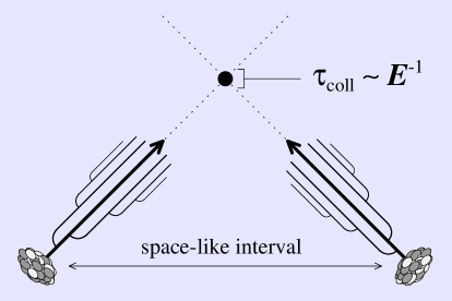
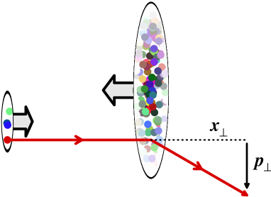
Figure 15: Left: The space–time picture of a high–energy collisions, illustrating the factorization of the cross–section. Right: particle production in a proton–nucleus (or ‘dilute–dense’) collision.

Even in this case, one needs to distinguish between two types of factorizations, depending upon the kinematics of the final state:

• If the relevant values of $x$ are not that small (say $x\gtrsim 0.01$), then the parton evolution with decreasing $x$ can be neglected and one can use the collinear factorization : the partons are assumed to move collinearly with the incoming hadrons (that is, one neglects their ‘intrinsic’ transverse momenta $\sim{\Lambda_{{\rm QCD}}}$) and the parton distributions like $xg(x,\mu^{2})$ depend only upon the longitudinal momentum fractions and upon the transverse resolution $\mu^{2}$ (the ‘factorization scale’) of the hard, partonic, subprocess. The dependence upon $\mu^{2}$ reflects the DGLAP evolution with increasing virtuality $Q^{2}$. coll provides an example of collinear factorization.

• At smaller values of $x$, such that $\alpha_{s}\ln(1/x)\gtrsim 1$, the small–$x$ evolution becomes important, leading to an increase in the density of gluons and in their average transverse momentum. Because of that, the gluons cannot be considered as ‘collinear’ anymore : their distribution in transverse momenta must be explicitly taken into account. That is, one has to use the ‘unintegrated’ gluon distribution, whose evolution with $1/x$ is described by the BFKL equation, cf. eq:unintp. The corresponding factorization formula, known as $k_{T}$–factorization, involves a convolution over the transverse momenta of the participating gluons. This is in fact a limiting case of the CGC factorization to be described shortly — namely its dilute limit, in which the saturation effects can be neglected.

(ii) The dense regime corresponds to collisions which probe saturation effects in at least one of the incoming hadrons. This happens when the transverse momenta of some of the produced particles are comparable with the saturation momentum at the relevant values of $x$. In such a case, the partons from one projectile scatter off a dense gluonic system (a CGC) in the other projectile, so they typically undergo multiple scattering. This is a non–linear effect similar to saturation: each additional scattering represents a correction of order $\alpha_{s}n$ to the cross–section, which for $n\sim 1/\alpha_{s}$ is an effect of order one. (As usual, $n=n(x,k_{\perp})$ denotes the gluon occupation number in the dense projectile and is of $\mathcal{O}{(1/\alpha_{s})}$ when $k_{\perp}\lesssim Q_{s}(x)$.) So, when a parton scatters off a CGC, the multiple scattering series must be resummed to all orders. This resummation involves arbitrarily many insertions of the strong colour field $A^{\mu}_{a}$ which represents the CGC, which implies that the associated cross–section is sensitive to multi–gluon correlations ($n$–point functions of the field $A^{\mu}_{a}$ with $n\geq 2$). Clearly, the multiple scattering cannot be encoded in the (collinear of $k_{T}$) factorization schemes alluded to above, which involve only the respective 2–point functions — the parton distributions.

Fortunately, there is an important simplification which occurs at high energy and which permits to compute multiple scattering to all orders: an energetic parton is not significantly deflected by the scattering and thus can be assumed to preserve a straight line trajectory throughout the collision. This is known as the eikonal approximation. To explain it in a simple, but phenomenologically relevant, setting, consider first proton–nucleus (p+A) collisions, cf. fig:factor right. This is an example of a dense–dilute scattering, that is, a collision in which a projectile which is relatively dilute (the ‘proton’) and can therefore be treated in the collinear or the $k_{T}$ factorization, scatters off a dense target (the ‘nucleus’). Then the partons from the dilute projectile undergo multiple scattering off the strong colour field of the dense target. For the kinematical conditions at RHIC or the LHC, this ‘dense–dilute’ scenario is optimally realized in the case of particle production at forward rapidities, that is, in the fragmentation region of the proton (deuteron at RHIC).

To be specific, consider the production of a light quark with rapidity $y>0$ and semi–hard transverse momentum $p_{\perp}$. The production mechanism is as follows: a quark from the proton, with relatively large longitudinal momentum fraction $x_{1}=(p_{\perp}/\sqrt{s})\rme^{y}$ and negligible transverse momentum, scatters off the gluons with $x_{2}\simeq(p_{\perp}/\sqrt{s})\rme^{-y}$ and $k_{2\perp}\sim Q_{s}(x_{2})$ from the nucleus — which form a dense system because $x_{2}\ll 1$ and $A\gg 1$ — and thus accumulates a final transverse momentum $p_{\perp}\sim Q_{s}(x_{2})$. Within the CGC effective theory, the nucleus in a given scattering event is described as a classical colour field $A^{\mu}_{a}$, off which the quark scatters with the $S$–matrix

$$S_{\alpha\beta}=\langle\beta|\,{\rm T}\exp\Big{\{}i\int\rmd^{4}y{\mathcal{L}}_{\rm int}(y)\Big{\}}|\alpha\rangle\quad\mbox{with}\quad{\mathcal{L}}_{\rm int}(y)=j^{\mu}_{a}(y)A_{\mu}^{a}(y)\quad\mbox{and}\quad j^{\mu}_{a}(y)=g\bar{\psi}\gamma^{\mu}t^{a}\psi\,.$$ (30)

Here ${\mathcal{L}}_{\rm int}(y)$ is the Lagrangian density for the interaction between the colour current $j^{\mu}_{a}$ of the quark and the colour field $A_{\mu}^{a}$ of the target, and $\alpha$ ($\beta$) represents the ensemble of the quantum numbers characterizing the state of the quark prior to (after) the collision. The quark deflection angle reads $\theta\simeq p_{\perp}/E_{1}$ with $E_{1}=x_{1}\sqrt{s}/2$ (the quark energy). For the kinematics of interest we have $p_{\perp}\ll E_{1}$, so this angle is small, $\theta\ll 1$, as anticipated. Hence, one can assume that the quark keeps a fixed transverse coordinate $\bm{x}_{\perp}$ while crossing the nucleus. This is the eikonal approximation. In this approximation, $\alpha=(\bm{x}_{\perp},i)$ and $\beta=(\bm{x}_{\perp},j)$, where $i$ and $j$ are colour indices in the fundamental representation of SU$(N_{c})$ which indicate the quark colour states before and respectively after the scattering. Also, assuming the quark to be a left–mover (and hence the nucleus to be a right mover, as in YM), one can write $j^{\mu}_{a}(y)\simeq\delta^{\mu-}gt^{a}\delta(y^{+})\delta^{(2)}(\bm{y}_{\perp}-\bm{x}_{\perp})$. Then Seik reduces to

$$\langle\bm{x}_{\perp},j|\,S\,|\bm{x}_{\perp},i\rangle\,\simeq\,V_{ij}(\bm{x}_{\perp})\quad\mbox{with}\quad V(\bm{x}_{\perp})\,\equiv{\rm T}\exp\Big{\{}ig\int\rmd x^{-}A^{+}_{a}(x^{-},\bm{x}_{\perp})t^{a}\Big{\}}\,,$$ (31)

where the ‘path–ordering’ symbol T denotes the ordering of the colour matrices $A^{+}_{a}(x^{-},\bm{x}_{\perp})t^{a}$ in the exponent, from right to left, in increasing order of their $x^{-}$ arguments. The integration runs formally over all the values of $x^{-}$, but in reality this is restricted to the longitudinal extent of the nucleus, which is localized near $x^{-}=0$ because of Lorentz contraction. The path–ordered exponential $V$ is a colour matrix in the fundamental representation, also known as a Wilson line. It shows that the only effect of the scattering in the high energy limit is to ‘rotate’ the colour state of the quark while the latter is crossing the nucleus. If instead of a quark, one would consider the scattering of a gluon, the corresponding $S$–matrix would be again a Wilson line, but in the adjoint representation ($t^{a}\to T^{a}$). When the target field is weak, $gA^{+}\ll 1$, one can expand the exponential in Wilson in powers of $gA^{+}$, thus generating the multiple scattering series. But when $gA^{+}\sim 1$, as is the case for a target where the gluons are at saturation, such an expansion becomes useless, since all the terms count on the same order. In such a case, one has to work with the all–order result, as compactly encoded in the Wilson line.

The above considerations also show that multiple scattering at high energy is most conveniently treated in the transverse coordinate representation: the successive collisions modify the transverse momentum of the partonic projectile, but do not significantly alter its transverse coordinate (or ‘impact parameter’). But the interesting observable is the cross–section for producing a quark (or gluon) with a given transverse momentum $p_{\perp}$ and rapidity $y$. This is obtained by multiplying the amplitude $V_{ij}(\bm{x}_{\perp})$ with the complex conjugate amplitude $V_{ji}^{\dagger}(\bm{y}_{\perp})$ for a quark at a different impact parameter $\bm{y}_{\perp}$, and then taking the Fourier transform $\bm{x}_{\perp}-\bm{y}_{\perp}\to\bm{p}_{\perp}$. This yields (for the forward kinematics of interest here)

$$\frac{\rmd N_{q}}{\rmd y\,\rmd^{2}\bm{p}_{\perp}}\,\simeq\,x_{1}f_{q}(x_{1},p_{\perp}^{2})\int\rmd^{2}\bm{r}_{\perp}\,\rme^{-i\bm{r}_{\perp}\cdot\bm{p}_{\perp}}\,\frac{1}{N_{c}}\left\langle{\rm tr}V(\bm{x}_{\perp})V^{\dagger}(\bm{y}_{\perp})\right\rangle_{Y}.$$ (32)

The quark distribution $x_{1}f_{q}(x_{1},p_{\perp}^{2})$ gives the probability to find a quark ‘collinear’ with the proton, with longitudinal momentum fraction $x_{1}$, on the resolution scale $p_{\perp}^{2}$ set by the partonic scattering. Within the integral, we have defined $\bm{r}_{\perp}\equiv\bm{x}_{\perp}-\bm{y}_{\perp}$. Furthermore, the colour trace has been generated by summing over the final colour indices ($\sum_{j}$) and averaging over the initial ones ($(1/N_{c})\sum_{i}$), and the brackets denote the average over the target wavefunction, evolved up to the rapidity $Y=\ln(1/x_{2})$. In the CGC formalism, this target average is computed according to average, that is, as an average over the colour charge density of the ‘fast’ sources which are responsible for the target field $A^{+}_{a}(x^{-},\bm{x}_{\perp})$ via YM:

$$S_{Y}(\bm{x}_{\perp},\bm{y}_{\perp})\,\equiv\,\frac{1}{N_{c}}\left\langle{\rm tr}V(\bm{x}_{\perp})V^{\dagger}(\bm{y}_{\perp})\right\rangle_{Y}=\int{\mathcal{D}}\rho\,W_{Y}[\rho]\,\,\frac{1}{N_{c}}\,{\rm tr}\big{(}V(\bm{x}_{\perp})V^{\dagger}(\bm{y}_{\perp})\big{)}\,.$$ (33)

This 2–point function of the Wilson lines is recognized as the $S$–matrix for the scattering between a colour dipole (a quark–antiquark pair in an overall colour singlet state) and the CGC. The non–linear effects enter this $S$–matrix at two levels: (i) via multiple scattering for the quark and the antiquark, as described by the respective Wilson lines, and (ii) via gluon saturation in the target wavefunction, as encoded in the CGC weight function. In this context, the target saturation momentum $Q_{s}(A,Y)$ also plays the role of the unitarization scale for the colour dipole: the dipole scattering becomes strong (meaning that $|S_{Y}(r_{\perp})|\ll 1$) when the dipole size $r_{\perp}$ is of order $1/Q_{s}$ or larger. Indeed, so long as the dipole is relatively small, such that $r_{\perp}\ll 1/Q_{s}$, it predominantly scatters off the gluon modes with $k_{\perp}\sim 1/r_{\perp}\gg Q_{s}$, which are dilute. The corresponding target field is weak ($gA^{+}\ll 1$), the Wilson lines are close to one, and so is the dipole $S$–matrix. Namely, for $r_{\perp}Q_{s}\ll 1$ one finds $1-S_{Y}(r_{\perp})\propto\big{(}r_{\perp}^{2}Q_{s}^{2}(Y)\big{)}^{\gamma_{s}}$ with $\gamma_{s}\simeq 0.63$. On the other hand, a large dipole with $r_{\perp}\gtrsim 1/Q_{s}(Y)$ probes the high–density gluon modes with $k_{\perp}\lesssim Q_{s}(Y)$; the associated colour fields are strong, $gA^{+}\sim 1$, so the Wilson lines are rapidly oscillating and their product averages out to a very small value: $|S_{Y}(r_{\perp})|\ll 1$ when $r_{\perp}Q_{s}\gg 1$.

The dipole $S$–matrix provides a convenient framework to study high energy evolution and saturation since, in the limit where the number of colours is large $N_{c}\gg 1$, it obeys a relatively simple equation for the evolution with $Y$ — a non–linear generalization of the BFKL equation known as the Balitsky–Kovchegov (BK) equation [24]. Originally deduced within Mueller’s ‘dipole picture’ [28, 9] (an insightful reformulation of the BFKL evolution valid at large $N_{c}$), the BK equation also emerges from the large–$N_{c}$ limit of the Balitsky–JIMWLK hierarchy. Remarkably, the BK equation is presently known to next–to–leading order (NLO) accuracy [29, 30, 31]. This is important in view of phenomenological studies of both deep inelastic scattering — at high energy, the DIS cross–section sigmagamma can be related to the dipole $S$–matrix [32] and the NLO corrections are essential in order to achieve a good description of the HERA data at small $x$ [33, 34, 35, 36, 37] — and of particle production in dense–dilute scattering, which is the topics of interest for us here.

Specifically, Eqs. quarkprod–aveWilson express the CGC factorization for inclusive quark production in dense–dilute scattering [38, 39, 40, 11]. quarkprod is usually written as

$$\frac{\rmd N_{q}}{\rmd y\,\rmd^{2}\bm{p}_{\perp}}\,\simeq\,\frac{\alpha_{s}}{p_{\perp}^{2}}\,x_{1}f_{q}(x_{1},p_{\perp}^{2})\,\Phi_{A}(Y,\bm{p}_{\perp},\bm{b}_{\perp}),$$ (34)

where the first factor $\alpha_{s}/{p_{\perp}^{2}}$ is the cross–section for the elementary $q+g\to q$ scattering (the would-be partonic subprocess in the single scattering limit) while

$$\Phi_{A}(Y,\bm{p}_{\perp},\bm{b}_{\perp})\equiv\frac{p_{\perp}^{2}}{\alpha_{s}}\int\rmd^{2}\bm{r}_{\perp}\,\rme^{-i\bm{r}_{\perp}\cdot\bm{p}_{\perp}}\,\frac{1}{N_{c}}\left\langle{\rm tr}V(\bm{x}_{\perp})V^{\dagger}(\bm{y}_{\perp})\right\rangle_{Y},$$ (35)

plays the role of a generalized unintegrated gluon distribution (here, for the nucleus) at impact parameter $\bm{b}_{\perp}=(\bm{x}_{\perp}+\bm{y}_{\perp})/2$. When $p_{\perp}\gg Q_{s}(A,Y)$, Phi can be evaluated in the single scattering approximation, as obtained by expanding the product of Wilson lines to quadratic order in $A^{+}$. In that (dilute) regime, $\Phi_{A}$ reduces indeed to the usual unintegrated gluon distribution — the one which enters the $k_{T}$–factorization and obeys the BFKL equation. But for lower momenta $p_{\perp}\lesssim Q_{s}(A,Y)$, the non–linear effects become essential, as already discussed in relation with the dipole scattering.

  

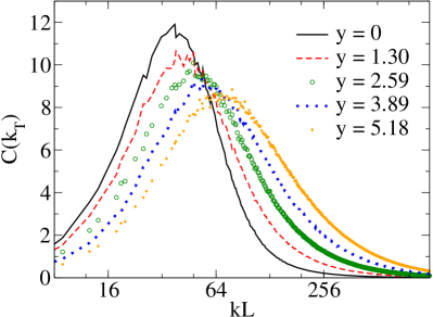
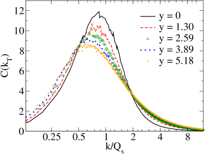
Figure 16: The results of the JIMWLK evolution for the generalized gluon distribution in Phi, parameterized as $\Phi(Y,\bm{k}_{\perp})\equiv(1/{\alpha_{s}})C(Y,\bm{k}_{\perp})$. Left: as a function of $k_{\perp}L$, with $L$ the transverse size of the system. Right: as a function of the scaling variable $k_{\perp}/Q_{s}(Y)$, to exhibit geometric scaling (the curves corresponding to different values of $Y$ fall approximately on top of each other). From Ref. [26].

fig:Phi shows the CGC prediction for the generalized gluon distribution Phi, as obtained via the numerical resolution of the JIMWLK equation with initial conditions at $Y=0$ of the McLerran–Venugopalan type (and with a running coupling) [26]. The two plots exhibit a pronounced peak at a special value of the transverse momentum $p_{\perp}$ which increases with $Y$ : this special value is, of course, the saturation momentum $Q_{s}(A,Y)$. In fact, it is quite easy to understand these plots in the light of our previous discussion of the dipole scattering. The Fourier transform in Phi is controlled by the competition between the complex phase $\rme^{-i\bm{r}_{\perp}\cdot\bm{p}_{\perp}}$ and the dipole $S$–matrix $S_{Y}(r_{\perp})$. For large momenta $p_{\perp}\gg Q_{s}$, the complex exponential limits the integration to small dipole sizes $r_{\perp}\lesssim 1/p_{\perp}\ll 1/Q_{s}$, for which the scattering is weak: $1-S_{Y}(r_{\perp})\sim\big{(}r_{\perp}^{2}Q_{s}^{2}(Y)\big{)}^{\gamma_{s}}$. Then the Fourier transform yields

$$\Phi_{A}(Y,p_{\perp})\,\simeq\,\frac{1}{\alpha_{s}}\left(\frac{Q_{s}^{2}(A,Y)}{p_{\perp}^{2}}\right)^{\gamma_{s}}\qquad\mbox{for}\quad p_{\perp}\gg Q_{s}(A,Y).$$ (36)

The difference $1-\gamma_{s}\simeq 0.37$ is an anomalous dimension introduced by the high energy evolution. (Without this evolution, one would have the bremsstrahlung spectrum $\propto 1/p_{\perp}^{2}$, cf. eq:unintp.) For lower momenta $p_{\perp}<Q_{s}$, the integral over $r_{\perp}$ in Phi is limited by the dipole $S$–matrix to values $r_{\perp}\lesssim 1/Q_{s}<1/p_{\perp}$. (Recall that $S_{Y}(r_{\perp})\ll 1$ when $r_{\perp}\gg 1/Q_{s}$.) Then

$$\Phi_{A}(Y,p_{\perp})\,\simeq\,\frac{p_{\perp}^{2}}{\alpha_{s}}\int\rmd^{2}\bm{r}_{\perp}\,\Theta\big{(}1/Q_{s}-r_{\perp}\big{)}\,\simeq\,\frac{1}{\alpha_{s}}\,\frac{p_{\perp}^{2}}{Q_{s}^{2}(A,Y)}\qquad\mbox{for}\quad p_{\perp}\lesssim Q_{s}(A,Y)\,.$$ (37)

Eqs. scaling and Philow explain the pronounced peak in the gluon distribution at $p_{\perp}\simeq Q_{s}(Y)$, as visible in fig:Phi. This in turn implies that the cross–section for particle production is dominated by semi–hard gluons with $p_{\perp}\sim Q_{s}(Y)$ and hence can be computed in perturbation theory. Another important consequence of saturation, which is visible too in Eqs. scaling and Philow (and is numerically tested in the right panel of fig:Phi), is geometric scaling [41, 42, 43, 44]: the unintegrated gluon distribution depends upon the two kinematical variables $p_{\perp}$ and $Y$ only via the dimensionless ratio $p_{\perp}/Q_{s}(Y)$. This scaling has important consequences for the phenomenology, to be discussed in the next section.

Note also that, as a result of the non–linear physics, the generalized ‘gluon distribution’ Phi is a process–dependent quantity : it depends not only upon the gluon density in the target, but also upon the nature of the partonic subcollision. For instance, if instead of the quark production, one would consider the production of a gluon, the ‘fundamental’ Wilson lines in Phi would be replaced by ‘adjoint’ ones [38, 39, 40]. Also, if one considers a more complicated final state — say, the production of a pair of partons — then the analog of Phi will involve a pair of Wilson lines for each of the partons partaking in the collision (one such a line in the direct amplitude and another one in the complex conjugate amplitude). More examples in that sense can be found in Refs. [45, 46, 47, 48, 49, 50]. See also [51] for a recent, comprehensive, discussion of the relation between the CGC factorization and the $k_{T}$–factorization. These considerations show that, in the presence of non–linear effects, the notion of ‘parton distribution’ ceases to be useful: the observables involve higher $n$–point functions of the gluon fields (generally, via the product of Wilson lines) which moreover couple with each other under the non–linear, JIMWLK, evolution. The complete information about the gluon correlations and their evolution with $Y$ (to leading–logarithmic accuracy at least) is encoded in the CGC weight function.

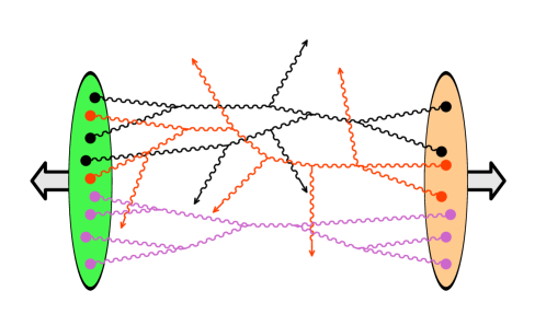
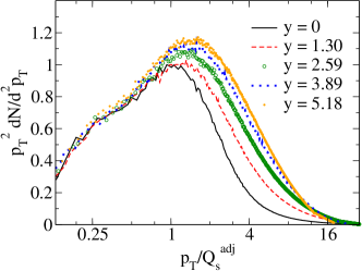
Figure 17: Left panel: a cartoon of the ‘dense–dense’ collision between two heavy nuclei, which illustrates the complexity of the process. Non–linear effects enter via gluon saturation (in both nuclei) and multiple scattering. Right panel: the gluon spectrum generated by this collision within the CGC formalism (from Ref. [26]).

We now turn to nucleus–nucleus ($A+A$) collisions, which for the typical kinematical conditions at RHIC and the LHC represents an example of dense–dense scattering : the wavefunctions of both nuclei develop saturation effects which influence the production of particles with semi–hard transverse momenta. Hence, in order to compute the bulk of particle production, one must take into account the many–body correlations associated with gluon saturation in both nuclei, together with the multiple scattering between these two saturated gluon distributions. Once again, this complex problem can be addressed within the CGC formalism and in the eikonal approximation. Not surprisingly, the treatment of the two nuclear projectiles is now symmetric: they are both described as colour glass condensates, with weight functions $W_{Y_{1}}[\rho_{1}]$ and, respectively, $W_{Y_{2}}[\rho_{2}]$. And their collision is described as the scattering between two classical distributions of colour charges moving against each other.

To be more specific, consider inclusive gluon production in the COM frame, where the nuclei have rapidities $\pm y_{\rm beam}$. If the produced gluon has rapidity $y$, it will probe the evolutions of the two nuclear wavefunctions up to rapidities $Y_{1}=y_{\rm beam}-y$ and $Y_{2}=y_{\rm beam}+y$, respectively. This motivates the following CGC factorization for the spectrum of the produced gluons [52]

$$\left\langle\frac{\rmd N}{\rmd y\,\rmd^{2}\bm{p}_{\perp}}\right\rangle\,=\int[\mathcal{D}{\rho_{1}}\mathcal{D}{\rho_{2}}]\,{W_{y_{{\rm beam}-y}}[\rho_{1}]}\,{W_{y_{{\rm beam}+y}}[\rho_{2}]}\,\frac{\rmd N}{\rmd y\,\rmd^{2}\bm{p}_{\perp}}\bigg{|}_{\rm class},$$ (38)

where the last factor inside the integrand, $({\rmd N}/{\rmd y\rmd^{2}\bm{p}_{\perp}})|_{\rm class}$, represents the spectrum produced in the scattering between two given configurations of classical colour sources (the ‘fast partons’) — one for each nucleus. More precisely, as discussed in relation with YM, the right–moving nucleus is described in a given event as a colour current having only a ‘plus’ component: $J^{\mu,a}_{1}=\delta^{\mu+}\rho^{a}_{1}$, with the charge density $\rho_{1}^{a}$ localized near $x^{-}=0$ (due to Lorentz contraction) and independent of $x^{+}$ (by Lorentz time dilation). Similarly, the left–moving nucleus is represented by a colour current with only a ‘minus’ component: $J^{\mu,a}_{2}=\delta^{\mu-}\rho^{a}_{2}$, with $\rho_{2}^{a}$ localized near $x^{+}=0$ and independent of $x^{-}$. At a classical level, the ‘scattering’ between these two currents is described by the solution $A^{\mu}_{a}$ to the Yang–Mills equation including both types of sources (compare to YM) :

$$D_{\nu}^{ab}F_{b}^{\nu\mu}(x)\,=\,\delta^{\mu+}\rho^{a}_{1}(x^{-},\bm{x}_{\perp})+\delta^{\mu-}\rho^{a}_{2}(x^{+},\bm{x}_{\perp})\,.$$ (39)

This equation describes multiple scattering because it is non–linear: the collision begins at $x^{+}=x^{-}=0$ (i.e. $t=z=0$) and for positive values of $x^{+}$ and $x^{-}$, the solution $A^{\mu}_{a}$ is non–linear to all orders in both $\rho_{1}$ and $\rho_{2}$. This solution cannot be computed analytically, but numerical solutions are by now available [53, 54, 55, 26]. The cross–section $({\rmd N}/{\rmd y\rmd^{2}\bm{p}_{\perp}})|_{\rm class}$ for particle production is obtained via the Fourier transform of this classical solution, that is, by projecting the field $A^{\mu}_{a}$ onto modes with transverse momentum $\bm{p}_{\perp}$. Finally, the average over the CGC weight functions of the two nuclei, cf. CGCfact, is numerically performed. It is this last procedure which introduces the dependence of the cross–section upon the rapidity $y$, via the corresponding dependence of the two weight functions. Note that, in line with the general philosophy of the CGC formalism, the only quantum effects to be included in the calculation are those associated with the high–energy evolution of the projectile wavefunctions prior to scattering, which are enhanced by the large logarithms $Y_{i}=\ln(1/x_{i})$, with $i=1,\,2$. The final outcome of this calculation is the gluon spectrum displayed in fig:AA (right panel) [26]. This is very similar to the ‘unintegrated’ gluon distribution in any of the incoming nuclei (compare to fig:Phi), in particular, it is peaked at a value of $p_{\perp}$ of the order of the saturation momentum and which increases with $y$. Some further consequences of the solution to YMAA will be discussed in sec:glasma.

Note finally an important difference between p+A (dilute–dense) and A+A (dense–dense) collisions: in the former, the particles produced by the collision do not interact with each other, but merely evolve via fragmentation and hadronisation towards the final hadrons observed in the detectors; by contrast, in A+A collisions the partonic medium created in the early stages of the collisions is very dense, so these partons keep interacting with each other — one then speaks about final state interactions, as opposed to the initial state ones, which were associated with high density effects like saturation in the incoming wavefunctions. These ‘final state’ interactions redistribute the partons in energy and momentum, which makes it difficult to verify the early–stages spectrum, as given by the aforementioned CGC calculations, against the measured hadron yield. Yet, the CGC formalism has the virtue to provide the initial conditions for the subsequent dynamics, at a time $\tau\simeq 1/Q_{s}\sim 0.2$ fm/c. So, its predictions can be at least indirectly tested, via calculations of the final state effects which include initial conditions of the CGC type. We shall return to such issues later on.

3.6 Some experimental signatures of the CGC in HIC

Let us consider now some phenomenological applications of the previous results for ‘dilute–dense’ scattering [10, 11, 14, 15] (and Refs. therein). We start with the $R_{pA}$ ratio, defined as the ratio between particle production in p+A collisions and that in p+p collisions for the same kinematics; schematically,

$$R_{pA}(\eta,p_{\perp})\,\equiv\,\frac{1}{N_{coll}}\,\frac{\frac{\rmd N_{h}}{\rmd^{2}p_{\perp}\rmd\eta}\Big{|}_{pA}}{\frac{\rmd N_{h}}{\rmd^{2}p_{\perp}\rmd\eta}\Big{|}_{pp}}\,,$$ (40)

where the subscript $h$ denotes the hadron species and $N_{coll}$ is the number of binary proton–nucleon collisions in the p+A scattering at a given impact parameter, as computed under the assumption that the various nucleons inside the nucleus scatter independently from each other. For relatively central collisions (i.e. small impact parameters; see fig:geometry), one has $N_{coll}\simeq A^{1/3}$. The normalization in RpA is such that $R_{pA}$ would be equal to one if the p+A collision was a superposition of $A$ incoherent p+p collisions. Conversely, any deviation in $R_{pA}$ from unity is an indication of coherence (high–density) effects in the nuclear wavefunction. Such a deviation is clearly seen in the respective RHIC data at forward rapidities ($\eta>0$). More precisely, RHIC performed deuteron–gold (d+Au) collisions at $\sqrt{s}=200$ GeV per nucleon pair and measured the ratio $R_{\rm d+Au}$ for semi–hard momenta $p_{\perp}=1\div 5$ GeV and for rapidities $\eta=0\div 4$ in the deuteron fragmentation region [56, 57].

The results of the corresponding analysis by BRAHMS are shown in fig:dAu. For $p_{\perp}\gtrsim 2$ GeV, they show an enhancement ($R_{\rm d+Au}>1$) for $\eta=0$, known as the ‘Cronin peak’, which however disappears when increasing $\eta$, leading to suppression ($R_{\rm d+Au}<1$) at $\eta>1$. E.g. for $\eta=3.2$, one finds $R_{\rm d+Au}\simeq 0.6\div 0.8$ for $p_{\perp}=2\div 4$ GeV. This behaviour can be understood in terms of saturation in the nuclear gluon distribution and its evolution with $Y$ [58, 59, 60, 61]. For central rapidities $\eta\simeq 0$ and $p_{\perp}=2$ GeV, one probes $x_{2}\sim 10^{-2}$, which is large enough for the high–energy evolution to be negligible. Then the gluon density in the nucleus is large juste because of the many ($3A$) valence quarks acting as sources for gluon radiation. An incoming parton from the deuteron scatters off this dense gluonic system and thus acquires an additional transverse momentum of order $Q_{s}(A,x_{2})\sim 1$ GeV. This yields a shift in the spectrum of the produced particles towards higher values of $p_{\perp}$, leading to the Cronin peak. For forward rapidities, say $\eta=3.2$ and $p_{\perp}=2$ GeV, one has $x_{2}\sim 10^{-4}$ and then the high–energy evolution with $Y=\ln(1/x_{2})$ is important. In that case, one can use the factorization ktfact for both d+Au and for the p+p collision which serves as a benchmark, leading to

$$R_{\rm d+Au}\,\simeq\,\frac{1}{A^{1/3}}\,\frac{\Phi_{A}(Y,p_{\perp})}{\Phi_{p}(Y,p_{\perp})}\,.$$ (41)

For this kinematics, the saturation effects are important in the gold nucleus (since the nuclear saturation scale $Q_{s}(A,Y)\sim 2$ GeV is comparable with $p_{\perp}$) and lead to a slow down of the evolution with $Y$. On the other hand, saturation is still negligible for the proton, so the corresponding unintegrated gluon distribution $\Phi_{p}(Y,p_{\perp})$ rises rapidly with $Y$, according to the BFKL evolution. Hence, when increasing $\eta$ (and thus $Y$), the denominator in dAu rises much faster than the numerator there, leading to a decrease in the ratio. This is precisely the trend seen in the data.

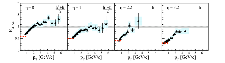
Figure 18: BRAHMS results for d+Au collisions at 200 GeV/nucleon [56] : the ratio $R_{\rm dAu}$ for charged hadrons as a function of $p_{\perp}$ for central and forward pseudorapidities.

In particular, for sufficiently high $Y$, such that both the nucleus and the proton in the ratio in dAu are at saturation, and for transverse momenta comparable or slightly larger to the nuclear saturation momentum ($p_{\perp}\gtrsim Q_{s}(A,Y)\simeq A^{1/3}Q_{s}(p,Y)$), one can use scaling for the unintegrated gluon distributions in both targets. This yields a particularly simple result,

$$R_{\rm d+Au}\,\simeq\,\frac{1}{A^{1/3}}\,\left(\frac{Q_{s}^{2}(A,Y)}{Q_{s}^{2}(p,Y)}\right)^{\gamma_{s}}\,\simeq\,A^{-\frac{1-\gamma_{s}}{3}}\,,$$ (42)

which is independent of both the transverse momentum (within a limited range above the nuclear saturation momentum) and the rapidity. It would be interesting to test this prediction in p+A collisions at the LHC, where the coverage in both $Y$ and $p_{\perp}$ will be larger than at RHIC.

Another important consequence of saturation, which is manifest in Eqs. scaling–Philow and has been implicitly used in deriving dAuscaling, is geometric scaling in the gluon distribution. Via ktfact, this suggests a similar scaling in the spectrum of the produced particles. This prediction has been tested against the LHC data for p+p collisions [62], with the results shown in fig:ptscaling. There one can see the ratio

$$R_{E_{1}/E_{2}}(p_{\perp},Y)\,=\,\frac{\big{(}{\rmd N}/{\rmd^{2}p_{\perp}\rmd\eta}\big{)}\big{|}_{E_{1}}}{\big{(}{\rmd N}/{\rmd^{2}p_{\perp}\rmd\eta}\big{)}\big{|}_{E_{2}}}$$ (43)

between the measured spectra for single–inclusive charged hadron production at two COM energies, $E_{1}=\sqrt{s_{1}}$ and $E_{2}=\sqrt{s_{2}}$, and for midrapidities: $|\eta|\leq 2.4$. More precisely, one displays two such ratios, as obtained by combining the LHC data for three different energies: $\sqrt{s}=0.9,\,2.36,$ and 7 GeV. (Note that these energies are high enough for the saturation effects to be important in the proton wavefunction for $\eta\simeq 0$ and semi–hard transverse momenta.) If the spectrum $({\rmd N}/{\rmd^{2}p_{\perp}\rmd\eta})$ scales as a function of $\tau\equiv p_{\perp}/Q_{s}(Y)$, then the ratio ratio should be equal to one when plotted as a function of $\tau$. This expectation is indeed met by the data, as shown in the r.h.s of fig:ptscaling. At this point, it is worth noting that geometric scaling has been first observed in the HERA data for DIS [41] and that the experimental search for this remarkable behaviour has been inspired by the theoretical ideas about gluon saturation.

   

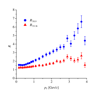
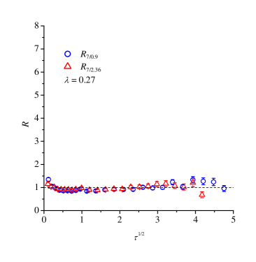
Figure 19: The ratio $R_{E_{1}/E_{2}}$ between particle spectra at energies $E_{1}$ and $E_{2}$, as measured for three energies at the LHC, is plotted as a function of $p_{\perp}$ (left panel) and of the scaling variable $\tau=p_{\perp}/Q_{s}(Y)$ (right panel). From Ref.[62].

Another remarkable regularity in the data which is naturally explained by the CGC is the limiting fragmentation : when the charged particle rapidity distribution $\rmd N/\rmd\eta$ is plotted as a function of the variable $\eta^{\prime}=\eta-y_{\rm beam}$ — the rapidity difference between the produced particle and the dilute projectile (say, the deuteron in the case of d+Au collisions) —, then the distribution turns out to be independent of the collision energy over a wide range around $\eta^{\prime}=0$, whose extent is increasing with $\sqrt{s}$ (see limfrag). Note that $\eta^{\prime}\simeq 0$ corresponds to forward rapidities ($\eta>0$) according to our previous terminology, to which ktfact applies. Moreover, for such rapidities, even a nucleus–nucleus collision may be viewed as ‘dilute–dense’, in the sense that one of the nuclei is probed at large $x_{1}$, where it looks dilute.

To understand limiting fragmentation on the basis of ktfact, notice that (i) $\eta-y_{\rm beam}\simeq\ln x_{1}$ (the rapidity of the produced particle is roughly equal to that of the fast parton which initiated the scattering), (ii) the ‘multiplicity’ $\rmd N/\rmd\eta$ is obtained by integrating the spectrum ktfact over all values of $\bm{p}_{\perp}$, (iii) this integral is dominated by $p_{\perp}\sim Q_{s}(Y)$ (since the gluon distribution is strongly peaked at $Q_{s}$, cf. fig:Phi), and (iv) the result of the integration is very weakly dependent upon $Y=\ln(1/x_{2})$, by geometric scaling (indeed, $\Phi_{A}(Y,p_{\perp})$ is roughly a function of $\tau\equiv p_{\perp}/Q_{s}(Y)$, which is evaluated at $\tau=1$ when performing the integral). These arguments imply that $\rmd N/\rmd\eta$ depends upon $x_{1}\simeq\exp(\eta-y_{\rm beam})$ but is approximately independent of $x_{2}$ (and hence of the total collision energy) within the range of ‘forward rapidities’. This is precisely the property called limiting fragmentation, as visible in limfrag for both d+Au and Au+Au collisions at RHIC (PHOBOS) [63, 64].

 

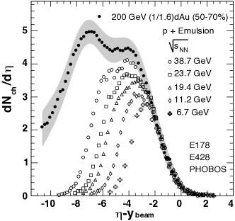
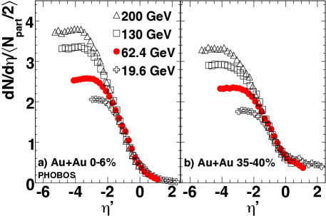
Figure 20: Pseudorapidity density distributions of charged particles emitted in d+Au collisions (left panel) and Au+Au collisions (right panel, separately for central and peripheral impact parameters), at various energies, as a function of the $\eta^{\prime}=\eta-y_{\rm beam}$ variable. In the right panel, the impact parameter is represented by the centrality bins: 0-6% (i.e. the 6% most central data) and respectively 35-40%. From Ref. [64].

As a final application for ‘dilute–dense’ scattering, we shall consider the production of a pair of hadrons at forward rapidities. The kinematics has been already explained in relation with 2pkin : when both $\eta_{a}$ and $\eta_{b}$ are positive and large, the produced hadrons explore small values $x_{2}\ll 1$ in the target wavefunction and hence they can experience high density effects — multiple scattering and gluon saturation. As before, these effects are important when the transverse momenta $p_{a\perp}$ and $p_{b\perp}$ of the two hadrons are comparable to the target saturation momentum. The respective cross–section admits a factorization similar to quarkprod, where however the target expectation value now involves the trace of the product of four Wilson lines: two for the produced partons in the direct amplitude, and two for the same partons in the complex conjugate amplitude. Hence, the generalized ‘gluon distribution’ of Phi gets now replaced by a 4–point function, known as a colour quadrupole [47, 48, 49, 50, 22].

A convenient way to study high–density effects in this setup is to measure di–hadron correlations in the azimuthal angle, which is the angle indicating the direction of propagation in the transverse plane. If the medium effects are negligible, two relatively hard particles ($p_{\perp}\gg\Lambda_{{\rm QCD}}$) are produced back–to–back ($\bm{p}_{a\perp}+\bm{p}_{b\perp}\simeq 0$). So, if the trigger detects one of these particles together with its fragmentation products (a ‘jet’), then by measuring the particle distribution in the same event one should find another ‘jet’ at a relative angle $\Delta\Phi\simeq\pi$. On the other hand, if the target looks dense on the transverse resolution scale of the produced particles, then the $p_{\perp}$–distribution gets broaden via multiple scattering and the peak corresponding to the ‘away jet’ at $\Delta\Phi\simeq\pi$ gets smeared, or it even disappears.

 

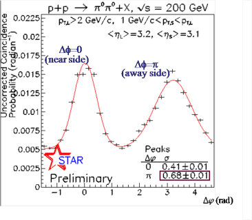
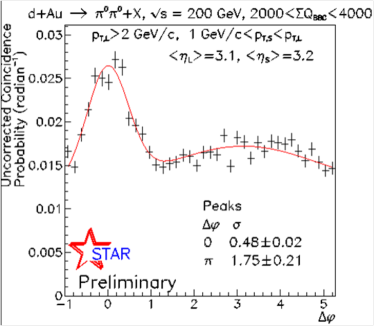
Figure 21: Di–hadron azimuthal correlations at forward rapidities ($\eta_{a},\,\eta_{b}\simeq 3$) and semi–hard transverse momenta as measured in p+p (left panel) and d+Au (right panel) collisions at RHIC, for $\sqrt{200}$ GeV per nucleon pair.

This scenario has been indeed confirmed by the RHIC data as measured by STAR [65, 66]. fig:dijet shows the experimental results for di–hadron production at forward rapidities ($\eta_{a,b}\simeq 3$) and semi–hard transverse momenta in both p+p and d+Au collisions. As already discussed in relation with RpA, for this kinematics one expects the saturation effects to be negligible for a proton target, but important for a gold nucleus. And indeed, the data for azimuthal correlations in fig:dijet show a pronounced ‘away’ peak in the p+p collisions (the left panel), but a strongly suppressed one in the d+Au ones (the right panel). Such a suppression was actually predicted by the CGC effective theory [49, 67] and its experimental observation at RHIC is one the most compelling evidences in favour of gluon saturation available so far.

Figure 22: The LHC data (ALICE [68]) for the midrapidity ($\eta=0$) charged particle multiplicity in Pb+Pb collisions at $\sqrt{s}=2.76$ TeV/nucleon pair, normalized by the number of participants $N_{\rm part}$ and plotted as a function of $N_{\rm part}$ — hence of the centrality of the collisions, which increases (meaning that the impact parameter $b_{\perp}$ decreases) with increasing $N_{\rm part}$. The predictions of six theoretical calculations are also shown. The three lowest ones, marked as ‘Armesto et al’, ‘Kharzeev et al’, and ‘Albacete et al’, are inspired by the CGC effective theory and explicitly include gluon saturation. The three other models include some of the effects of saturation, in the form of an energy–dependent ‘infrared’ cutoff at low transverse momenta, $p_{\perp}^{\rm min}\sim E^{\lambda}$, which effectively plays the role of $Q_{s}$.

Turning to A+A (or ‘dense–dense’) collisions, we recall that, in that case, the CGC framework provides the initial conditions for the subsequent evolution of the liberated partonic matter, but not also the spectrum of the produced hadrons. Still, predictions can be more for more inclusive quantities like the total multiplicity, which are expected to be less affected by ‘final state’ interactions. In particular, fig:multipli exhibits the centrality dependence of the multiplicity of the charged particles as measured at the LHC in Pb+Pb collisions at $\sqrt{s}=2.76$ TeV/nucleon pair, together with the respective predictions of various theoretical models. The centrality of a collision refers to the relative impact parameter $b_{\perp}$ of the two projectiles in the transverse plane (see fig:geometry). For A+A collisions, this is often parameterized in terms of the ‘number of participants’ — the number of incoming nucleons from the two nuclei in the region where the nuclei overlap with each other (the ‘interaction region’). Clearly, central collisions ($b_{\perp}\simeq 0$) involve more participants than the peripheral (large $b_{\perp}$) ones. Although one cannot compute $\rmd N_{\rm ch}/\rmd\eta$ fully from first principles (as this also requires some information about the distribution of nucleons within the nuclear disk), one can easily estimate the dependence of this quantity upon $N_{\rm part}$ within the framework of the CGC effective theory. As discussed in relation with fig:AA, the partons produced in the early stages of a A+A collision are typically gluons with transverse momenta $p_{\perp}\sim Q_{s}$, which have been liberated by the collision. So the multiplicity $\rmd N_{\rm ch}/\rmd\eta$ near $\eta=0$ is proportional to the number of such gluons which were present in the initial nuclei, within their region of overlapping:

$$\frac{\rmd N_{\rm ch}}{\rmd\eta}\Big{|}_{\eta=0}\,\propto\,S\,\frac{xg_{A}(x,Q_{s}^{2})}{\pi R_{A}^{2}}\,\propto\,\frac{1}{\alpha_{s}(Q_{s}^{2})}\,S\,Q_{s}^{2}(A,E)\,\sim\,N_{\rm part}\,E^{\lambda}\ln\frac{Q_{s}^{2}(A,E)}{\Lambda_{{\rm QCD}}^{2}}\,.$$ (44)

Here, $S$ is the transverse area of the interaction region and we have used Qsat for the (nuclear) saturation momentum together with the fact that $S\,Q_{s}^{2}(A,E)$ is proportional to $N_{\rm part}$ and it grows with the COM energy $E=\sqrt{s}$ like $E^{\lambda}$ (cf. QsxA and the discussion of fig:multiplicity). Hence, the ratio $(\rmd N_{\rm ch}/\rmd\eta)/N_{\rm part}$ is expected to be only weakly dependent upon $N_{\rm part}$, via the corresponding dependence of the running coupling: $1/{\alpha_{s}(Q_{s}^{2})}\sim\ln({Q_{s}^{2}}/{\Lambda_{{\rm QCD}}^{2}})\sim\ln N_{\rm part}$. This is in good agreement with the data, as shown in fig:multipli. (For the most refined calculation to date, whose results are indicated in fig:multipli by the curve denoted as ‘Albacete et al’, see Ref. [69].)

Figure 23: A sketch of the geometry of a heavy ion collision. The collision (or longitudinal) axis is denoted as $z$, while $x$ and $y$ are the transverse coordinates. The interaction region (the almond–shape region where the two nuclei overlap which each other) is singled out. $N_{\rm part}$ is the number of nucleons in this region. The interaction region is horizontally cut by the reaction plane $(x,z)$.

3.7 The Glasma

By the uncertainty principle, it takes a time $\Delta t\sim 1/Q_{s}$ to liberate a particle with transverse momentum $p_{\perp}\sim Q_{s}$ at midrapidities ($\eta\simeq 0$). So, by that time, the small–$x$ gluons which were originally confined within the wavefunctions of the incoming nuclei, are released by the collision. What is the subsequent evolution of these gluons ? To answer this question one needs a better understanding of their configuration at the time of emission. This can be inferred from the solution $A^{\mu}_{a}$ to the Yang–Mills equation YMAA, or, more precisely of the associated chromo–electric and magnetic fields, ${\bm E}_{a}$ and ${\bm B}_{a}$.

Prior to the collision ($t<0$), these fields describe the two ‘colour glass condensates’ of the incoming nuclei, which by causality are independent of each other. Due to the high–energy kinematics, the CGC fields turn out to be quite simple (see fig:sheet) : for each nucleus, the respective vectors ${\bm E}_{a}$ and ${\bm B}_{a}$ have only transverse components, $E^{i}_{a}$ and $B^{i}_{a}$ with $i=1,2$, meaning that they are orthogonal to the collision axis $x^{3}$. Besides, they are also orthogonal to each other, ${\bm E}_{a}\cdot{\bm B}_{a}=0$ (for each of the $N_{c}^{2}-1=8$ values of the colour index $a$), and they have equal magnitudes:

$${\bm E}_{a}\,\perp\,{\bm B}_{a}\,\perp\,x^{3},\quad|{\bm E}_{a}|\,=\,|{\bm B}_{a}|\qquad\mbox{(prior to the collision)}\,.$$ (45)

These initial electric and magnetic fields are localized near $x^{-}=0$ for the left–moving nucleus and, respectively, $x^{+}=0$ for the right–moving one, like the respective colour charges. In a given event, their values and orientations can randomly vary from one point to the other in the transverse plane. But on the average, the fields at different points are correlated due to ‘memory’ effects in the high energy evolution, in particular, due to saturation. The correlations, which are encoded in the respective CGC weight functions, are typically restricted to a saturation disk, i.e. to transverse areas with radius $\sim 1/Q_{s}$ : domains separated by transverse distances $\Delta x_{\perp}\gg 1/Q_{s}$ evolve independently from each other, since saturation prohibits the emission of gluons with momenta $k_{\perp}\ll Q_{s}$. Within a saturation disk, gluons arrange themselves in such a way to shield their colour charges and thus minimize their mutual repulsion; accordingly, a saturation disk has zero overall colour charge (see the right figure in fig:hadron). Also, gluons can be correlated with each other in rapidity, due to the fact that they have common ancestors, i.e. they belong to the same parton cascade. Such correlations extend over a rapidity interval $\Delta Y\sim 1/\alpha_{s}$, since this is the typical value of $Y$ which is required to build parton cascades according to the BFKL evolution. These correlations, which were built in the initial wavefunctions via the high–energy evolution, get transmitted to the gluons liberated by the collision and thus have consequences for the distribution of the particles in the final state.

In view of the above, a A+A collision can be viewed as the scattering between two sheets of coloured glass, as illustrated in fig:sheet. Incidentally, a similar structure for the incoming fields — electric and magnetic fields which are orthogonal to the beam axis and to each other, and which are localized near the respective light–cone and frozen by Lorentz time dilation — would also hold if the nuclei were made with electric (rather than colour) charges. In both QED and QCD, such field configurations — known as the Weizsäcker–Williams fields — represent the boosted version of the Coulomb fields created by the ensemble of (electric or colour) charges in their rest frame. However, the non–Abelian structure of QCD is essential for having a collision: the Abelian version of YMAA would be linear and it would not describe a scattering process. (The total electromagnetic field at $t>0$ would be simply the sum of the individual fields of the two nuclei.) The non–linear effects encoded in the Yang–Mills equation YMAA describe the scattering between the small–$x$ gluons in the two CGC’s. The corresponding solution at $t>0$ (more precisely, in the forward light cone at $x^{+}>0$ and $x^{-}>0$, which is the space–time region causally connected to the collision) represents the gluonic matter produced by the collision.

This solution exhibits a very interesting structure: in addition to the transverse fields on the two sheets, which after the collision are separating from each other, there are also longitudinal, electric and magnetic fields, $E^{3}_{a}$ and $B^{3}_{a}$, which extend along the collision axis. The latter give rise to colour flux tubes (or ‘strings’) with the endpoints on the two sheets and a typical transverse radius $1/Q_{s}$ (see fig:flux left). Right after the collision ($t=0_{+}$), these fields are quite strong, $E^{3}\sim B^{3}\sim 1/g$, since they carry most of the energy of the original CGC fields. At such early times, the gluonic matter is still in a high–density, coherent state, for which a description in terms of classical fields is better suited than one in terms of particles. But with increasing time, the system expands, its density decreases, and so does the strength of the fields. After a time $t\sim 1/Q_{s}$, the magnitudes of all the fields (transverse and longitudinal) becomes of order one, meaning that, from now on, these fields can be also interpreted as incoherent superpositions of particles. The spectrum of these particles (mostly gluons) is obtained from the Fourier modes of the colour fields at time $t\gtrsim 1/Q_{s}$. These particles can interact with each other, as their density is still quite high (albeit decreasing with time, due to expansion). As we shall see, these interactions are expected to lead to a phase of local thermal equilibrium — the quark–gluon plasma (QGP).

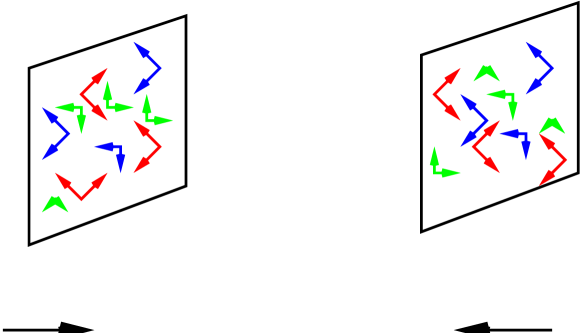
Figure 24: The chromo-electric and chromo-magnetic field configurations in the two nuclei prior to the collision.

The intermediate, non–equilibrium, form of matter, which interpolates between the CGC in the initial wavefunctions and the QGP at later stages is known as the glasma (a name coined as a combination of ‘glass’ and ‘plasma’) [70]. The main, qualitative, feature of the glasma is the presence of longitudinal colour flux tubes with transverse area $\sim 1/Q_{s}^{2}$, which are boost invariant : the colour fields depend upon the proper time $\tau$ but not also upon the space–time rapidity $\eta_{s}$. The variables $\tau$ and $\eta_{s}$, which can be used instead of $t$ and $z\equiv x^{3}$ in the forward LC, are defined as

$$\tau\,=\,\sqrt{t^{2}-z^{2}}\,,\qquad\eta_{s}\,=\,\frac{1}{2}\,\ln\frac{t+z}{t-z}\,\Longrightarrow\,\tanh\eta_{s}\,=\,\frac{z}{t}\,.$$ (46)

Under a boost along the $z$ axis, $\tau$ is invariant while $\eta_{s}$ is shifted by a constant. Lines of constant $\tau$ and of constant $\eta_{s}$ are shown in fig:flux (right). The fact that the glasma fields depend upon $\tau$ but not upon $\eta_{s}$ is a consequence of the symmetries of the collision, as encoded in the classical field equations YMAA. This is also consistent with the hypothesis of uniform longitudinal expansion, as originally formulated by Bjorken. Specifically, Bjorken has assumed that (i) after being produced at $t\simeq z\simeq 0$, the particles undergo free longitudinal streaming, meaning that they keep a constant velocity along the $z$ axis; accordingly, the particles that can be found at some later time $t$ at point $z$ are those with a longitudinal velocity $v_{z}=z/t$; (ii) the distribution of the produced particles is uniform in $v_{z}$. Together, (i+ii) imply that the distribution at time $t$ is independent of $z/t$, hence of $\eta_{s}$. Note that this argument identifies the momentum rapidity $y$ (cf. ydef) of the produced particles with their space–time rapidity $\eta_{s}$ : $\tanh y\equiv v_{z}=z/t\equiv\tanh\eta_{s}$. Hence, the boost invariance of the glasma fields implies that the distribution of the particles produced by the decay of these fields is independent of $y$. This is a generic feature of the particle production at the classical level, that is, on an event-by-event basis: the associated spectra are boost invariant. But the physical spectra, as obtained after averaging the classical results with the CGC weight functions of the incoming nuclei, cf. CGCfact, are rapidity–dependent, because of the respective dependencies of the weight functions, as introduced by the quantum evolution with $Y$.

 

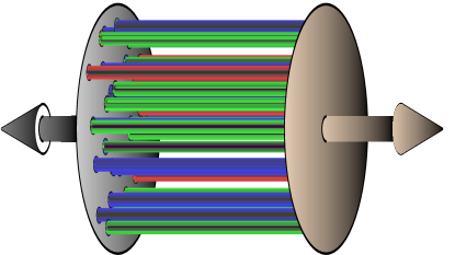
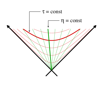
Figure 25: Left: the longitudinal colour flux tubes which develop in between the remnants of the two nuclei in the early stages ($\tau\lesssim 1/Q_{s}$) of a A+A collision. Right: various choices of coordinates in the future light cone.

An interesting consequence of the above considerations, which might be related to a remarkable phenomenon seen in the RHIC [71, 72, 73, 74] and the LHC data [75, 76, 77] and known as the ridge, refers to the rapidity dependence of the two particle correlation. The latter is defined as

$$C_{2}(\eta_{a},\bm{p}_{a\perp};\eta_{b},\bm{p}_{a\perp})\,=\left\langle\frac{\rmd N_{2}}{\rmd\eta_{a}\rmd^{2}\bm{p}_{a\perp}\,\rmd\eta_{b}\rmd^{2}\bm{p}_{b\perp}}\right\rangle-\left\langle\frac{\rmd N}{\rmd\eta_{a}\rmd^{2}\bm{p}_{a\perp}}\right\rangle\left\langle\frac{\rmd N}{\rmd\eta_{b}\rmd^{2}\bm{p}_{b\perp}}\right\rangle\,,$$ (47)

and what is generally plotted is the ratio $\mathcal{R}$ between this correlation and is disconnected part (below, $N_{a}$ denotes the number of particles of type $a$ in a given bin in pseudo–rapidity and azimuthal angle),

$$\mathcal{R}\,\equiv\,\frac{\langle N_{a}\,N_{b}\rangle-\langle N_{a}\rangle\,\langle N_{b}\rangle}{\langle N_{a}\rangle\,\langle N_{b}\rangle}\,,$$ (48)

as a function of the rapidity and the azimuthal separations between the two particles, $\Delta\eta=\eta_{a}-\eta_{b}$ and $\Delta\phi=\phi_{a}-\phi_{b}$. Remarkably, the data for A+A collisions at both RHIC and the LHC show the existence of correlations which extend over a large rapidity interval $\Delta\eta\simeq 4\div 8$, but restricted to small azimuthal separations $\Delta\phi\simeq 0$ (see fig:ridge left). This means that particles which propagate along very different directions with respect to the collision axis preserve nevertheless a common direction of motion in the transverse plane. By causality, such a correlation must have been produced at early times, when these particles — which rapidly separate from each other — were still causally connected (see the right panel of Fig. 26). A simple estimate gives

$$\tau_{\rm max}=\tau_{\rm freeze-out}\;\rme^{-\frac{|\Delta\eta|}{2}}\;,$$ (49)

for the latest time at which these particles could have been correlated. For a freeze–out time $\tau_{\rm freeze-out}\approx 10~{}$fm/c, and rapidity separations $\Delta\eta\geq 4$, one sees that these correlations must have been generated before $1~{}$fm/c.

Long–range rapidity correlations are natural in the glasma picture, where all the spectra (in particular, the 2–particle ones) are independent of $y$ — at least, at the classical level. After averaging with the CGC weight functions, as in CGCfact, the 2–particle spectrum acquires a dependence upon the average rapidity of the two particles $(\eta_{a}+\eta_{b})/2$, but not upon their difference $\Delta\eta$. This last argument remains correct so long as one can neglect quantum corrections due to soft gluon emissions within the rapidity interval $\Delta\eta$, which in turn requires $\Delta\eta\lesssim 1/\alpha_{s}$. Concerning the azimuthal collimation of the ridge, this is not a consequence of the glasma — the particles produced via the decay of the classical fields are emitted isotropically in the transverse plane in the rest frame of the medium —, but can be generated via radial flow : the local fluid element has some transverse velocity $\bm{v}_{\perp}$, which introduces a bias in the azimuthal distribution of the particles produced by the decay of a same flux tube (the final correlation is peaked around the direction of $\bm{v}_{\perp}$). Flow phenomena will be discussed in more detail in the next section.

 

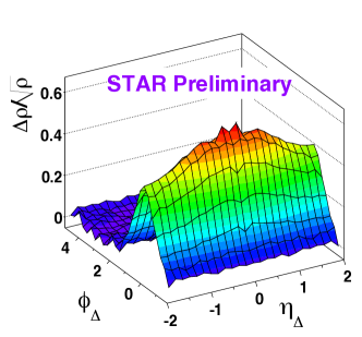
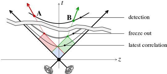
Figure 26: Left: the ‘ridge’ in the di–hadron correlations as measured by RHIC (STAR). Right: the causal structure of the di–hadron rapidity correlations; the 2 hadrons $A$ and $B$ propagating with different rapidities were causally connected in the space–time region where the respective backward light–cones with vertices on the freeze–out surface were overlapping with each other.

For sufficiently high energy, the long–range rapidity correlations invoked for A+A collisions should be also present in the p+p collision. In that case, one expects no flow, as there are fewer produced particles and the freeze–out time is shorter. Yet, a small ridge has been measured in p+p collisions by the CMS collaboration at the LHC [78], but only in the high–multiplicity events (which are believed to be more central) and within a limited range in $p_{\perp}$ (from 1 to 3 GeV), which is in the ballpark of the proton saturation momentum at the LHC. In that case, the azimuthal collimation could be explained by an intrinsic angular correlation between the emission of two particles from the glasma field [79].

Let us also note another possible consequence of the glasma flux tubes: the presence of longitudinal electric and magnetic fields implies the existence of topologically non–trivial configurations, characterized by a large density of Chern–Simons topological charge. Such configurations are interesting in that they break the charge–parity (CP) symmetry: via the chiral anomaly, they generate a difference between the number of quarks with right–handed and respectively left–handed helicity. In the context of HIC, they may generate a new phenomenon, known as the chiral magnetic effect [80] : quarks with opposite helicities can be separated by the ultra strong magnetic fields ($B\sim 10^{18}$ Gauss) created in the peripheral ultrarelativistic A+A collisions, thus leading to a charge asymmetry between the two sides of the reaction plane. Since the direction of the magnetic field varies from one collision to another, this effect leads to fluctuations in the distribution of the electric charge of the final hadrons. These theoretical expectations appear to be supported by measurements at RHIC (STAR) [81].

4 The Quark Gluon Plasma

The main topic of this chapter is the quark–gluon plasma (QGP) — the partonic form of QCD matter in thermal equilibrium which exists for sufficiently large temperatures, as demonstrated by numerical calculations in lattice QCD. This form of matter is expected to be created during the intermediate stages of a ultrarelativistic HIC, albeit only for a short lapse of time and in a state of only local thermal equilibrium. We shall first review the main experimental evidence in favour of QGP in a HIC, namely the observation of flow in the particle production and its successful description in terms of hydrodynamics. Then we shall discuss the QGP thermodynamics from the viewpoints of lattice theory and perturbative QCD. We shall also mention the difficulty of perturbation theory to describe the dynamics out-of-equilibrium (in particular, the transport coefficients and the process of thermalization). Then we shall consider the phenomenon of jet quenching (the energy loss by an energetic parton via interactions in the plasma), which is an important tool for exploring the deconfined matter produced in HIC’s. At several places in what follows, we shall encounter situations where perturbation theory appears to be insufficient and which may signal a regime of strong coupling. To address such situations from the opposite limit — that of a coupling which is arbitrarily strong —, one can rely on techniques borrowed from string theory, via the AdS/CFT correspondence. This will be briefly discussed (in relation with the physics of HIC’s) in the last section of these lectures.

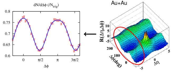
Figure 27: The double–peak structure characteristic of elliptic flow: two wide peaks at $\Delta\phi=0$ and $\Delta\phi=\pi$ which extend over a wide interval $\Delta\eta$ in rapidity. The strong correlation peak visible at $(\Delta\phi,\Delta\eta)\simeq(0,0)$ is associated with the fragmentation of the trigger jet.

4.1 Correlations and flow in HIC

In our previous discussion of the ‘ridge’, in sec:glasma, we focused on the long–range rapidity correlations which are rather strongly peaked in $\Delta\phi=\phi_{a}-\phi_{b}$ near $\Delta\phi=0$, leading to the ressemblance with a mountain ridge. But as a matter of fact, the di–hadron correlations measured in A+A collisions at RHIC and the LHC show an even more pronounced double–peak structure, visible in fig:ridge-flow, with large but wider peaks at $\Delta\phi=0$ and $\Delta\phi=\pi$. (In the analysis leading to fig:ridge, this structure has been subtracted away to render the ridge effect visible.) This is known as elliptic (or ‘transverse’) flow [82]. As also visible in fig:ridge-flow, this double peak structure can be well parameterized as

$$\left\langle\frac{\rmd N_{pairs}}{\rmd\Delta\phi}\right\rangle\,\propto\,v_{2}^{2}\,\cos(2\Delta\phi)\,,$$ (50)

with $v_{2}$ the ‘magnitude of the elliptic flow’.

The explanation of this phenomenon turns out to be quite simple: it reflects the anisotropy of the interaction region — the almond–shape region where the two nuclei overlap with each other; see fig:geometry — for non–central collisions. This anisotropy entails a pressure gradient in the initial conditions: the pressure is larger along the minor axis of the ellipse (the $x$ axis in the left panel of fig:ellipse) rather than along the major one; accordingly, more particles will be emitted in the direction of the largest gradient. This ultimately generates an anisotropy in the azimuthal distribution of the produced particles, which for symmetry reasons is of the form shown in v2:

$$\frac{\rmd N}{\rmd\phi}\,\propto\,1\,+\,2v_{2}\cos 2\phi\,.$$ (51)

This argument looks simple, as anticipated, but there is something deep about it: the role played by collective phenomena like pressure gradients or flow. Such phenomena are natural for many–body systems which relatively strong interactions — sufficiently strong to be able to transmit the asymmetry of the initial geometry into properties of the final state. This is an important point to which we shall return.

The qualitative arguments above suggests that the coefficient $v_{2}$ characterizing the strength of the anisotropy should increase with centrality. This trend is indeed seen in the data (at least, for not too peripheral collisions, for which the interaction region becomes tiny and dilute). Also, particles which experience a stronger pressure gradient are expected to have a larger transverse momentum, as they inherit the velocity of the fluid; so, $v_{2}$ should rise with $p_{\perp}$. This expectation, too, is confirmed by the data, at least for not too large $p_{\perp}\lesssim 5$ GeV: very hard particles cannot be driven by the medium, so for them $v_{2}$ is naturally small. The measurements of $v_{2}$ (say, via 2–hadron correlations) yield very similar results at RHIC and the LHC (see the left panel of fig:vn), showing that $v_{2}$ is roughly independent of the COM energy. Note also that the typical values of $v_{2}$ for semi–hard momenta are relatively large, $v_{2}\sim 0.2$, meaning that the collective phenomena alluded to above are indeed quite strong.

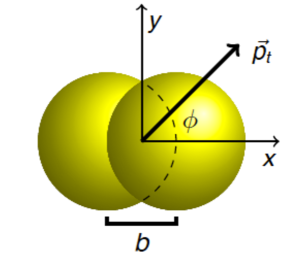
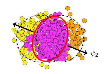
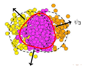
Figure 28: Left: a frontal view of a HIC, illustrating the impact parameter $b_{\perp}$, the almond–shape interaction region, and the azimuthal angle $\phi$. Central and right: the distribution of nucleons within the interaction region in a given event can include elliptic ($v_{2}$), triangular ($v_{3}$), or even higher harmonic modes. The reference angles $\psi_{2}$, $\psi_{3}$ show the tilt of the interaction region with respect to the geometrical ‘reaction plane’ (cf. fig:geometry).

But the elliptic flow and the ridge are not the only collective phenomena hidden in the di–hadron correlations illustrated in fig:ridge-flow. By looking at the most central collisions where $v_{2}$ is relatively small, one sees not only the narrow ‘ridge’ at $\Delta\phi\simeq 0$, but also a ‘double–hump’ on the away side, at $|\Delta\phi-\pi|\simeq 1.1$, which extends too over a large interval $\Delta\eta$ (see fig:hump left). The harmonic decomposition of this signal reveals higher Fourier modes with significant strengths, as illustrated in the right panel of fig:hump. This leads to the following generalization of flowv2 :

$$\left\langle\frac{\rmd N_{pairs}}{\rmd\Delta\phi}\right\rangle\,\propto\,1\,+\,2\sum_{n=1}^{\infty}\big{\langle}v_{n}^{2}\big{\rangle}\cos(n\Delta\phi)$$ (52)

where the various coefficients $v_{n}$ up to $v_{6}$ have been extracted from the LHC data and they are compared to $v_{2}$ in the right panel of fig:vn. (All these coefficients are roughly independent of $\eta$, meaning that they describe correlations over a wide interval $\Delta\eta$.)

What is the physics of such higher harmonics ? It is generally believed that they are the consequence of fluctuations in the distribution of nucleons within the interaction region, as illustrated in fig:ellipse (right panel) [83]. Namely, even though the overlapping region between the two nuclei has an elliptic shape, the nuclear matter inside it is neither homogeneous, nor strictly ellipsoidal, because of fluctuations in the particle distribution. The azimuthal distribution in a given event can be decomposed into harmonics, with coefficients $v_{n}$ and reference angles $\psi_{n}$ :

$$\frac{\rmd N}{\rmd\phi}\,\propto\,1\,+\,\sum_{n=1}^{\infty}2v_{n}\cos n(\phi-\psi_{n})\,.$$ (53)

The reference angles $\psi_{n}$ are generally different from the conventional reaction plane ($\psi_{RP}=0$) and are difficult to measure, but they drop out in the 2–particle correlations, as manifest in vn.

Figure 29: The ‘ridge’ at $\Delta\phi\simeq 0$ and the ‘double–hump’ at $|\Delta\phi-\pi|\simeq 1.1$ as visible in the LHC data for di–hadron correlations in the 5% most central collisions (left panel), together with the harmonic decomposition of these correlations, cf. vn (right panel) [84].

 

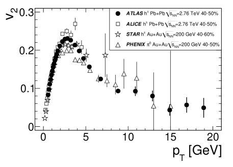
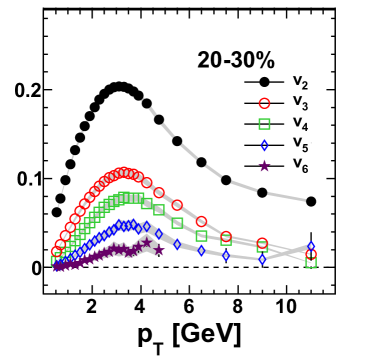
Figure 30: Left: the RHIC and LHC results for $v_{2}$ as a function of $p_{\perp}$, for collisions within the centrality bin $40\%-50\%$; from Ref. [85]. Right: the LHC results (ATLAS) for $v_{n}(p_{\perp})$, for $n=2,3,4,5$ and 6, and the centrality bin $20\%-30\%$ [84].

The fact that the initial geometry of the interaction region can have complicated fluctuations is not necessarily a surprise, given the granularity of the nucleons. What is remarkable though is the ability of the system to transmit these fluctuations into the distribution of the produced particles, via transverse flow. The effective theory for flow is hydrodynamics and will be succinctly discussed in the next section.

4.2 Hydrodynamics and kinetic theory

Hydrodynamics is the theory which describes the flow of a fluid independently of its detailed microscopic structure. More precisely, the equations of hydrodynamics have an universal form (at least, for a given underlying fundamental theory, like QCD), but they involve a few ‘parameters’ which depend upon the nature of the fluid and can in principle be computed via microscopic calculations. The scope of hydrodynamics can be most easily explained with reference to thermodynamics. The latter describes a many–body system in global thermal equilibrium, in which the intensive quantities, like temperature, pressure and the chemical potentials associated with the various conserved charges (electric charge, baryonic charge, etc) are time–independent and uniform throughout the volume $V$ of the system. Hydrodynamics can be viewed as a generalization of this picture towards a state of local equilibrium: the intensive quantities alluded to above can vary in space and time, but they do that so slowly that one can still assume thermal equilibrium to hold locally, in the vicinity of any point. Gradients of pressure and thermodynamics naturally lead to flow, with a local fluid velocity ${\bm v}$ which is itself slowly varying in space and time.

The equations of hydrodynamics are simply the ensemble of the relevant conservation laws — for the energy, momentum and the other conserved charges:

$$\partial_{\mu}\,T^{\mu\nu}\,=\,0\,,\qquad\partial_{\mu}J^{\mu}_{B}\,=\,0\,,\quad\cdots$$ (54)

where $T^{\mu\nu}$ is the energy–momentum tensor, $J^{\mu}_{B}$ is the density of the baryonic current (the volume integral of $J^{0}_{B}$ is the difference between the number of baryons and the number of antibaryons), and the dots stand for other conserved charges. These densities depend upon the intensive (local) quantities describing the state of the fluid: the energy density $\varepsilon=E/V$, the pressure $P$, the 4–velocity $u^{\mu}=\gamma(1,{\bm v})$ (with $\gamma=1/\sqrt{1-v^{2}}$), and a set of ‘friction coefficients’ known as viscosities, which characterize the dissipative properties of the medium.

The relations between the densities of the conserved charges ($T^{\mu\nu}$, $J^{\mu}_{B}$, …) and the intensive quantities are obtained via a gradient expansion with respect to the slow space–time variations of the latter. More precisely, this amounts to an expansion in powers of $\ell/R$, where $R$ is a characteristic size of the system (in a HIC, $R$ is the transverse size of the interaction region) and $\ell$ is the mean free path of the particles composing the fluid (the typical distance between two successive collisions). This quantity will play an important role in what follows, so let us open here a parenthesis and discuss it in more detail.

At least for sufficiently weak coupling, the mean free path $\ell$ can be estimated using kinetic theory. This is an effective theory too, but it applies at shorter, microscopic, scales: in that context, the mean free path is typically the largest scale in the problem (it is much larger than the Compton wavelength $\lambda\sim 1/k$ of a particle or the typical duration of a scattering processes). Kinetic theory allows one to follow the evolution of the particle distributions in phase–space — i.e. in space–time and in momentum space. To that aim, this theory involves more information about the microscopic dynamics, like cross–sections for the particles interactions described via the ‘collision term’ in the Boltzmann equation — the central equation of kinetic theory. But even without solving that equation, one can deduce an estimate for $\ell$ via simple considerations: the collision rate (the inverse of the typical time $\tau_{\rm coll}$ between two successive collisions) scales like $\tau^{-1}_{\rm coll}\sim nv_{\rm rel}\sigma$, where $n$ is the particle density, $v_{\rm rel}$ is their average relative velocity, and $\sigma$ is the cross–section for their mutual interactions. The mean free path is then obtained as

$$\ell\,\sim\,v\tau_{\rm coll}\,\sim\,\frac{v}{v_{\rm rel}n\,\sigma}\,\sim\,\frac{1}{n\,\sigma}\,,$$ (55)

where $v$ is the average velocity of the particles, so $v/v_{\rm rel}$ is a number of order one. Since $\sigma$ is naturally proportional to some power of the coupling constant, mfp shows that the mean free path becomes smaller — meaning that the hydrodynamical description works better — when the coupling is strong.

To be more specific, consider a system that will play an important role in what follows: a weakly coupled quark–gluon plasma with (local) temperature $T$. This is a nearly ideal gas of ultrarelativistic particles, so the particle densities scale like $n\sim T^{3}$ separately for quarks and gluons. To leading order in $\alpha_{s}$, scattering is controlled by the $2\to 2$ elastic collisions shown in fig:elastic, where the external lines represent thermal particles with typical energies and momenta of order $T$. These processes yield $\sigma\propto\alpha_{s}^{2}$. However, for the processes involving the exchange of a gluon in the $t$ channel, there is a logarithmic enhancement associated with the singularity of the Coulomb scattering at small angles: the Rutherford formula reads $\rmd\sigma/\rmd\Omega\propto\alpha_{s}^{2}/(T^{2}\sin^{4}\theta)$, with $\theta$ the scattering angle, and it is strongly divergent when $\theta\to 0$. The cross–section $\sigma$ which is relevant for computing the mean free path mfp is not the total cross–section $\sigma_{\rm tot}=\int\rmd\Omega\big{(}\rmd\sigma/\rmd\Omega\big{)}$, but rather the transport cross–section :

$$\sigma\,=\,\int\rmd\Omega\big{(}1-\cos\theta\big{)}\,\frac{\rmd\sigma}{\rmd\Omega}\,\propto\,\int\rmd\theta\,\sin\theta\big{(}1-\cos\theta\big{)}\,\frac{\alpha_{s}^{2}}{T^{2}\sin^{4}\theta}\,\sim\,\frac{\alpha_{s}^{2}}{T^{2}}\int_{g}\frac{\rmd\theta}{\theta}\,\sim\,\frac{\alpha_{s}^{2}}{T^{2}}\,\ln\frac{1}{\alpha_{s}}\,,$$ (56)

which more properly characterizes the efficiency of the interactions in redistributing energy and momentum. The factor $1-\cos\theta$, which vanishes as $\theta^{2}/2$ at small angles, accounts for the fact that the small–angle scattering is inefficient in that sense, as intuitive from the fact that one cannot equilibrate an anisotropic energy–momentum distribution via collinear scattering. Due to this factor, the integral in sigma is only logarithmically divergent as $\theta\to 0$ (unlike $\sigma_{\rm tot}$, which would be quadratically divergent). In reality, this divergence is screened by plasma effects which occur at the momentum scale $gT$ (see the discussion in sec:thermo). This implies that the minimal collision angles are $\theta\sim gT/T\sim g$, corresponding to transferred momenta of order $gT$. Hence, to leading logarithmic accuracy, the integral can be estimated as shown in the r.h.s. of sigma. In turn, this implies the following estimate for the mean free path in a weakly–coupled QGP (cf. mfp)

$$\ell\,\sim\,\frac{1}{T}\,\frac{1}{\alpha_{s}^{2}\ln(1/\alpha_{s})}\,,$$ (57)

which as long as $g\ll 1$ is indeed much larger than both the Compton wavelength $\lambda\sim 1/T$ of the thermal particles and the typical duration $\sim 1/gT$ of a scattering process.

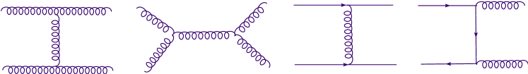
Figure 31: $2\to 2$ partonic processes dominating the cross–section for (elastic) scattering at weak coupling.

We now close the parenthesis dedicated to the mean free path and return to the discussion of hydrodynamics. As already mentioned, this is a legitimate effective theory for flow when $\ell\ll R$. The constitutive relation allows one to relate the energy–momentum tensor to the velocity field $u^{\mu}$ and its gradients, via an expansion in powers of $\ell/R$. The powers of $\ell$ are associated with dissipative phenomena, while those of $1/R$ with the gradients in the fluid. To zeroth order in this gradient expansion one obtains the ideal hydrodynamics. This is ‘ideal’ in the sense that there is no dissipation. The corresponding structure of $T^{\mu\nu}$ follows entirely from the assumption of local thermal equilibrium. Namely, in the local rest frame of a fluid element ($u^{\mu}_{RF}=(1,0,0,0)$), the energy–momentum tensor has the diagonal structure familiar from the thermodynamics: $T^{\mu\nu}_{RF}=\mbox{diag}(\varepsilon,P,P,P)$. Boosting to the laboratory frame, where the fluid 4–velocity is $u^{\mu}$, this yields

$$T^{\mu\nu}\,=\,(\varepsilon+P)u^{\mu}u^{\nu}-Pg^{\mu\nu}\,,$$ (58)

where $g^{\mu\nu}=\mbox{diag}(1,-1,-1,-1)$ is the Minkowski metric tensor. The r.h.s. of Tmunu involves 5 independent quantities: $\varepsilon$, $P$, and the 3 components $v^{i}$ of the (local) velocity. Their space–time evolution is determined by the respective conservation law in conservation, which yields 4 equations, together with the assumed equation of state, which specifies the functional relation $\varepsilon(P)$ between the energy density and the pressure (e.g., $\varepsilon=3P$ for an ideal gas of massless particles).

Since ideal hydrodynamics ignores dissipation, one might think that it corresponds to a situation where the coupling is weak, but that would be wrong: it rather corresponds to strong coupling. This may seem counterintuitive but it can be understood as follows: the dissipative phenomena are proportional to the ability of the system to transfer momentum in a direction perpendicular to the fluid velocity (since such a transfer results in slowing down the flow). Within kinetic theory at least, this transfer is realized by particles moving throughout the fluid in between successive collisions. Hence, the rate for transfer is proportional to the mean free path mfp and thus to the inverse of the coupling. As an example, consider the shear viscosity: this characterizes the friction force between two neighboring layers of fluid which propagate, say, along the $x$ axis, but at slightly different velocities (so there is a non–zero gradient $\partial u_{x}/\partial y$). There is friction because some longitudinal momentum $p_{x}$ gets transferred from the faster layer to the slower one, at a rate proportional to the velocity gradient:

$$\frac{1}{A}\,\frac{\rmd p_{x}}{\rmd t}\,=\,-\eta\,\frac{\partial u_{x}}{\partial y}\,,$$ (59)

where $A$ is the contact area between the two layers and $\eta$ is the shear viscosity. Within kinetic theory, $\eta\simeq\ell\rho v\sim(\rho/n)(v/\sigma)$ where $\rho$ is the mass density in the fluid and the second estimate follows after using mfp. For a non–relativistic fluid $\rho/n=m$, so $\eta\sim mv/\sigma$, whereas for the weakly–coupled QGP, $\rho=\varepsilon\simeq 3nT$ and $v=1$ and therefore

$$\eta\,\sim\,\frac{T}{\sigma}\,\sim\,\frac{T^{3}}{\alpha_{s}^{2}\ln(1/\alpha_{s})}\,.$$ (60)

In both cases, the fluid density has canceled in the ratio $\rho/n$, so the viscosity is independent of the density, or, equivalently, of the pressure. (Recall that $P=nk_{B}T$, with $k_{B}$ the Boltzmann constant.) This remarkable conclusion has been first derived by Maxwell in 1860 via kinetic theory, and then confirmed by him experimentally.

The l.h.s. of shear represents a contribution to the component $T_{xy}$ of the energy–momentum (or ‘shear’) tensor : the flux of the $x$ component of the momentum vector across a surface with constant $y$. So, shear displays a dissipative correction to $T_{\mu\nu}$ ; as expected, this is of linear order in the gradient expansion and it scales like $\ell/R$ (since $\eta\sim\ell$ and $\partial_{y}\sim 1/R$). While first–order gradient corrections (leading to the Navier–Stokes equation) are sufficient to describe dissipation for a non–relativistic fluid, this is not true anymore for a relativistic one: to be consistent with causality and Lorentz invariance, one must use a second–order formalism, which also includes quadratic terms in the gradient expansion.

To summarize, for the problem of hydrodynamics to be well defined, one needs to specify (i) the equation of state $\varepsilon(P)$ (this is generally taken from lattice QCD calculations; see below), (ii) the time $\tau_{0}$ at which hydrodynamical evolution can be turned on (meaning that local thermal equilibrium has been reached), (iii) the initial conditions at $\tau_{0}$ for the energy density $\varepsilon({\bm x})$ and the velocity ${\bm v}({\bm x})$ fields, and (iv) the various viscosities like $\eta$ which characterize the dissipative properties of the medium. Note that, in this context, the ‘initial time’ $\tau_{0}$ is not the same as the time $\tau_{s}\sim 1/Q_{s}$ at which the CGC formalism provides the ‘initial conditions’ (in the sense of the discussion in sec:glasma), but it is the a priori larger equilibration time $\tau_{\rm eq}$. Within the hydro simulations, this is a free parameter, like the viscosities or the parameters which enter the equation of state. These parameters are fixed a posteriori, by matching the results of the hydro evolution at the time of freeze–out onto some of the experimental results for particle production, like the centrality dependence of the particle multiplicities and of their average transverse momentum.

For quite some time, roughly until 2007, it seemed that the RHIC data can be well accounted for (within the error bars) by ideal hydrodynamics [86]. This led to the conjecture that the deconfined matter produced at the intermediate stages of a HIC might be strongly interacting (‘strongly coupled quark–gluon plasma’ or sQGP). In order to test this conjecture, and also to describe the more accurate, recent data, it became necessary to include dissipative effects, within the second–order formalism. Full calculations in that sense, including comparison with RHIC data, became available only recently [87, 88, 89] (and refs. therein). They are all consistent with a non–zero, albeit small, relative value of the viscosity, as measured by the ratio $\eta/s$. Here, $s$ is the entropy density, and the ratio $\eta/s$ is dimensionless in natural units (in general, it has the dimension of $\hbar$). This ratio is a natural measure of the deviations from ideal hydro, as we explain now. The entropy density $s$ is proportional to the particle density; e.g., $s=4n$ for an ideal gas of massless particles. Thus, $\eta/s\sim\ell v(\rho/n)\sim\ell/\lambda$, where $\lambda$ is the Compton wavelength of a particle in the fluid: $\lambda=1/(mv)$ in the non–relativistic case and $\lambda\sim 1/T$ for a weakly coupled QGP. By the uncertainty principle, the ratio $\ell/\lambda$ cannot be smaller than $\hbar$ times a number of $\mathcal{O}{(1)}$. So, the ratio $\eta/s$ cannot become arbitrary small, even when increasing the coupling. In that sense, a physical fluid can never be ideal.

An additional argument in that sense comes from the study of a strongly–coupled theory via the AdS/CFT correspondence. At least for the more symmetric, conformal, field theories to which it applies, this formalism predicts a lower bound on the ratio $\eta/s$, namely [90, 91] (the subscript ‘CFT’ refers to a conformal field theory; see sec:AdS for details)

$$\frac{\eta}{s}\bigg{|}_{\rm CFT}\,\geq\,\frac{\hbar}{4\pi}\,,$$ (61)

with the lower bound being reached in the limit of an infinitely strong coupling (in a sense to be characterized in sec:AdS). One remarkable thing about the heavy–ion data at RHIC and the LHC is that they seem to require a value $\eta/s$ almost as small as this absolute lower bound: $\eta/s\simeq 0.08\div 0.20$ depending upon the details of the ‘initial conditions’ at time $\tau_{0}$. (For instance, the analysis in Ref. [87] favors a value $\eta/s\simeq 0.16$ for initial conditions of the CGC type, as shown in the left panel of fig:hydro.) The other remarkable thing is that, in order to be successful, the hydro descriptions of the data must assume a very small equilibration time $\tau_{0}\lesssim 1$ GeV/c. These are both hallmarks of a system with strong interactions. Indeed, the particles thermalize by exchanging energy and momentum (and other quantum numbers) with each other, via their mutual collisions. So, we expect the thermalization time to be shorter for strongly interacting systems. This expectation is supported by kinetic theory, which yields a thermalization time $\tau_{\rm eq}\simeq\ell/v\propto[T\alpha_{s}^{2}\ln(1/\alpha_{s})]^{-1}$ to leading–order at weak coupling. For realistic values of $\alpha_{s}$, this perturbative estimate is too large to be consistent with the data (even when corrected for inelastic processes like $2\to 3$, which turn out to be important [92]).

 

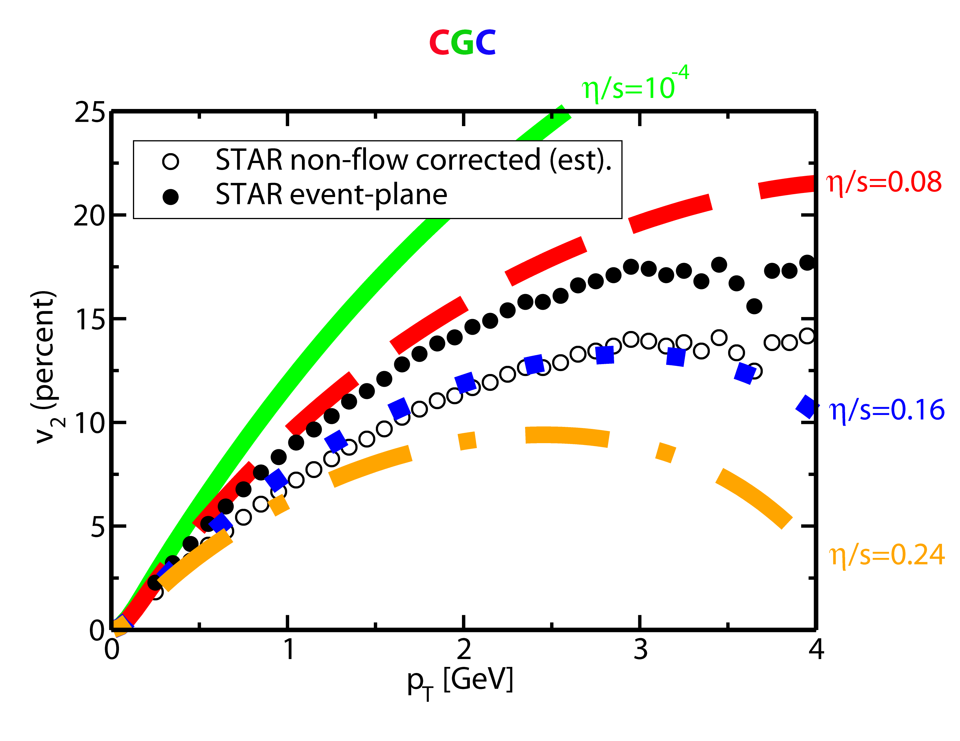
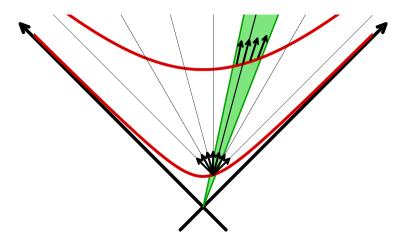
Figure 32: Left panel: the $v_{2}$ results of hydro calculations using the second order formalism with CGC initial conditions and various values of $\eta/s$ [87]. The comparaison with the RHIC data favors $\eta/s\simeq 0.16$, which is about twice the lower limit Soneta predicted by AdS/CFT at infinitely strong coupling. Right label: the longitudinal expansion has the tendency to collimate nearby particles, thus opposing to the evolution towards isotropy.

In the context of heavy ion collisions, the evolution towards (local) thermal equilibrium is furthermore hindered by the extreme anisotropy of the initial conditions and also by the anisotropy of the early–time expansion, which is predominantly longitudinal. Recall the glasma picture of the initial conditions (at times $\tau_{s}\sim 1/Q_{s}$), which is that of colour flux tubes extending along the collision $x$, cf. fig:flux. Flux tubes have an internal tension opposing to their longitudinal extension, like a string. Accordingly, the longitudinal component of the energy–momentum tensor associated with the glasma is negative ; one finds $T^{\mu\nu}_{\rm glasma}=\mbox{diag}(\varepsilon,\varepsilon,\varepsilon,-\varepsilon)$ at such early times, which is extremely anisotropic, as anticipated. Subsequent interactions among particles are supposed to restore isotropy, but this is rendered difficult by the longitudinal expansion, as illustrated in the right panel of fig:hydro. Namely, even if the particle distribution turns out to be locally isotropic at a given position in space and time, the subsequent anisotropic expansion rapidly separates the particles from each other according to the directions of their velocities: only those particles remain close to each other which had nearly parallel velocities. In other terms, by itself, the longitudinal expansion would naturally build a particle distribution in which nearby particles move along quasi–parallel directions, thus opposing isotropy. To beat this tendency and ensure isotropy, one needs strong interactions which continuously randomize the directions of motion of the particles. This would be natural at strong coupling, as alluded to above. But there are also other scenarios which are currently explored, including weak–coupling ones. One promising mechanism in that sense refers to plasma (Weibel) instabilities : due to the anisotropy of the expanding parton distribution, the soft colour fields radiated by these partons can develop unstable modes, that is, modes whose amplitudes grow exponentially with time (at least, during a limited time interval). So far, it is not clear whether this mechanism can lead to rapid isotropisation in the presence of longitudinal expansion, but its studies are under way (see Refs. [93, 94, 95, 96, 97, 98] for recent work and related references). Recent developments include a calculation (similar to previous work in inflationary dynamics) of the spectrum of initial quantum fluctuations in the glasma [95], a parametric analysis of the interplay between plasma instabilities and Bjorken expansion in the weak–coupling limit [96, 97], and an interesting scenario (still at weak coupling) in which the elastic scattering between the highly occupied glasma fields leads to the formation of a transient Bose–Einstein condensate [99].

4.3 QGP: Thermodynamics and collective excitations

In this section, we shall deviate from the experimental situation in HIC’s, where the partonic medium is rapidly expanding, and focus on a quark–gluon plasma at rest, in thermal and chemical equilibrium. The existence of such a deconfined phase in QCD at finite temperature has been unambiguously demonstrated via numerical calculations on a lattice, which have also given a lot of information about the thermodynamics of this system. Some of this information has been corroborated via analytic calculations at weak coupling, which turned out to be very non–trivial. The analytic methods become essential when one is interested in real–time phenomena, like the response of the system to time–dependent external perturbations, as characterized by transport coefficients. Indeed, real–time phenomena cannot be (easily) studied via lattice calculations, which are a priori formulated in a space–time with Euclidean signature (‘imaginary time’). It should be also stressed that, even though weak–coupling techniques appear to be quite successful in reproducing the lattice results for the QGP thermodynamics, the hypothesis that the coupling be strong is not yet totally excluded (within the temperature range relevant for the phenomenology at RHIC and the LHC): indeed, weak–coupling calculations seem unable to explain the small $\eta/s$ ratio supported by the data (cf. sec:hydro). In what follows, all that will be explained in some detail.

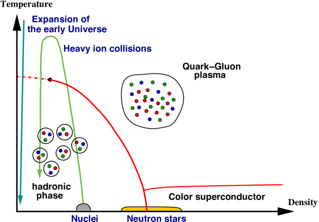
Figure 33: Schematic representation of the phase–diagram in QCD at finite temperature and non–zero quark density, as emerging from lattice calculations at zero (or small) quark density and from various theoretical considerations (like pQCD) in the other domains.

fig:phase shows a cartoon of the phase–diagram expected in QCD when varying the temperature $T$ and the net quark density (or the quark chemical potentials $\mu_{f}$), by which one means the difference between the density of quarks and that of the antiquarks. (For simplicity, fig:phase treats the three light quark flavors — the only ones to be relevant for the phase diagram — on the same footing.) This diagram has been actually demonstrated only in special corners, like the deconfinement phase transition with increasing $T$ at zero (or small) fermionic density, that has been established on the lattice, and the islands denoted as ‘nuclei’ or ‘neutron stars’, which are rather well understood within nuclear theory. The ‘colour superconductivity’ phase at high quark density, which is predicted by pQCD (at least for $\mu\gg\Lambda_{{\rm QCD}}$), will not be discussed here, as it is not expected to play any role in the ultrarelativistic HIC’s. (See the review papers [101, 102] and Refs. therein for detailed discussions of this phase.)

As also illustrated in fig:phase, the deconfinement phase transition has been first explored during the expansion of the Early Universe: the high temperature ‘soup’ of matter created right after the Big Bang was originally in the deconfined, QGP, phase; due to its rapid expansion, this matter has cooled down and thus crossed into the confined, hadronic, phase, at a very short time $\sim 10^{-5}$ seconds after the Big Bang. In the context of HIC’s, this transition is being probed the other way around: to start with, the partons are confined within the nucleons composing the two nuclei; the collision liberates these partons and, if their energy density is high enough, they can thermalize at a temperature superior to the critical temperature for deconfinement. If so, they form a transient QGP phase which cools down via expansion and eventually ‘evaporates’ into hadrons. In both scenarios, the net quark density is small and plays no role for the transition. In the Early Universe, the excess in the number of quarks over antiquarks was negligible (if any !) [103]. In HIC’s, there is of course a net baryon number, due to the $2A\simeq 400$ nucleons within the incoming nuclei; however, this excess is small compared to the number of hadrons (a few thousand) produced in the final state. This implies that most of the partons which exist in the intermediate stages of the collision are actually gluons or ‘sea’ quark–antiquark pairs.

 

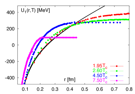
Figure 34: The quark–antiquark potential between two heavy quarks, as computed in QCD on the lattice. Left panel: $T=0$. Right panel: various temperatures, which are all larger than the critical temperature for deconfinement $T_{c}$ (for comparison, the $T=0$ potential is also shown, as the continuous line which keeps rising) [104].

The fundamental property of the QGP is, of course, deconfinement : quarks and gluons can move (more or less freely, depending upon their mutual interactions) throughout the whole volume of the plasma, without being confined within hadrons with radia $\sim 1/\Lambda_{{\rm QCD}}$. How is this possible ? A quark and an antiquark in isolation (i.e. at zero temperature) attract each other via a force which becomes roughly constant — corresponding to a linear potential; see fig:confinement left — at distances $r\gtrsim 1/\Lambda_{{\rm QCD}}$. Due to this force, the $q\bar{q}$ pair is tightly bound (‘confined’) into a meson. This meson can be broken, say, via a hard scattering, but only at the expense of producing additional gluons and $q\bar{q}$ pairs which ‘glue’ to the original quark and antiquark, in such a way to form colour singlet states (new hadrons). This is the situation in the ‘usual’ hadronic processes, including p+p collisions at the LHC, where the parton density right after the collision is not very high — so, these partons can evolve and eventually hadronize independently of each other. But in HIC’s, the density of the liberated partons is such that the typical interparticle separation is much shorter than $1/\Lambda_{{\rm QCD}}$. At such short distances, the attraction force between these partons is smaller than their kinetic energy, so the partons can move around each other and arrange themselves in such a way to minimize their mutual repulsion. The net result is that the colour charge gets screened over relatively short distances $r\ll 1/\Lambda_{{\rm QCD}}$, thus preventing the development of confining forces at larger distances.

This colour screening in the QCD plasma is very similar to electric (Debye) screening in ordinary, electromagnetic, plasmas, or in electrolytes. Ions with positive electric charge attract ions or electrons with negative charge, in such a way to form clouds of particles which look electrically neutral when seen from far away: the net charge decreases exponentially with the distance from the central charge (see fig:debye left). In the context of QCD, the ‘positive and negative electric charges’ are replaced by the $N_{c}^{2}-1=8$ ‘colour’ charges carried by quarks and gluons, but the exponential screening of the chromo–electric charges works in a similar way. As a consequence of that, the quark–antiquark potential flattens out (meaning that there is no attraction force) at large distances $r\gtrsim r_{D}$ with $r_{D}$ the Debye radius. This flattening is clearly seen in the lattice calculations at finite temperature (see e.g. the discussion in [104]), as illustrated in the right panel of fig:confinement. This also suggests that in a finite temperature plasma one cannot have quarkonia (bound states made with a heavy quark ($Q$) and a heavy antiquark ($\bar{Q}$), like $J/\psi$, with size $r_{Q\bar{Q}}>r_{D}$. This observation [105] led to the fertile idea of quarkonia melting in a quark–gluon plasma, a very active field of research for both theoretical (including lattice) and experimental studies of HIC’s. (See [106] for a recent overview of the theory and more references.)

 

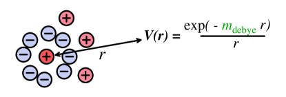
Figure 35: Left panel: illustration of the Debye screening in a QED plasma; the screening length is the inverse of the Debye ‘mass’: $r_{D}=1/m_{D}$. A similar mechanism is active in the QGP. Right panel: the Debye screening in QCD is the result of one–loop corrections due to the ‘hard’ ($k\sim T$) thermal particles (quark and gluons) which are resummed in the propagator of the ‘soft’ ($k\sim gT$) electric gluon exchanged between the quark and the antiquark.

The lattice calculations also allow one to study the deconfinement phase transition with increasing temperature. The respective results for the pressure and energy density are illustrated in fig:pressure. They show a sudden increase around a critical temperature $T_{c}\simeq 160\div 180$ MeV, interpreted as the result of the rise in the number of degrees of freedom (d.o.f.), due to the liberation of quarks and gluons. For $T\leq T_{c}$, the only ‘thermodynamically active’, hadronic d.o.f. (those whose masses are not much higher than $T$) are the 3 pions: $\pi^{0}$ and $\pi^{\pm}$. For $T>T_{c}$, this number jumps from 3 to 52: the gluons, which appear in 8 colours and 2 transverse polarizations ($8\times 2=16$ d.o.f.), and the 3 light quarks and antiquarks, each of them having 2 spin states and 3 possible colours ($3\times 3\times 2\times 2=36$ d.o.f.). Lattice calculations become more tedious for light quark masses and the extrapolation to physical quark masses has become possible only recently [107, 108]. This is important since both the actual value of the critical temperature and the nature of the phase transition are strongly influenced by the values of these masses. A phase transition is said to be of $n$th order if it involves a discontinuity in the derivative of order $(n-1)$ of the pressure. For instance, if the QCD phase transition was of first–order, then it would proceed via a mixed phase where hadronic bubbles coexist with regions of QGP. But this is not what happens in QCD: recent lattice calculations [109] show that, for physical quark masses, the deconfinement phase transition is truly a cross–over, that is, a relatively smooth process during which the pressure and all its derivatives remain continuous across the transition.

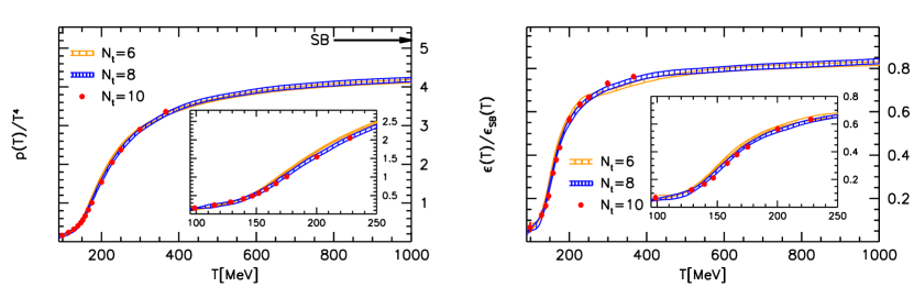
Figure 36: The lattice results (as obtained by the Budapest–Wuppertal collaboration [110]) for the QCD pressure and energy density as a function of the temperature.

But albeit smooth, the phase transition represents a genuinely non–perturbative phenomenon, which cannot be described within perturbative QCD. This can be appreciated e.g. by inspection of the lattice results for the trace anomaly $(\varepsilon-3P)/T^{4}$, which exhibit a sharp peak around $T_{c}$, as visible in the left panel of fig:trace. As mentioned in sec:hydro, $\varepsilon=3P$ for an ideal gas of massless particles, meaning that the corresponding energy–momentum tensor $T^{\mu\nu}=\mbox{diag}(\varepsilon,P,P,P)$ is traceless: $T^{\mu}_{\ \mu}=0$. This property is in fact a general consequence of conformal symmetry : it holds for any theory which involves no intrinsic mass parameter and hence is invariant under dilations. This is in particular the case for QCD with massless quarks at the classical level. However, at the quantum level, conformal symmetry in QCD is broken by the radiative corrections responsible for the running of the coupling, which introduce the mass scale $\Lambda_{{\rm QCD}}$. So, not surprisingly, the corresponding ‘trace anomaly’ (the deviation of $T^{\mu}_{\ \mu}$ from zero) is proportional to the $\beta$–function, which measures the running of the coupling :

$$T^{\mu}_{\ \mu}\,=\,\varepsilon-3P\,\,=\,\beta(g)\,\frac{\partial P}{\partial g}\,,\qquad\beta(g)\,\equiv\,\frac{\partial g}{\partial\ln\mu_{\rm ren}}\,.$$ (62)

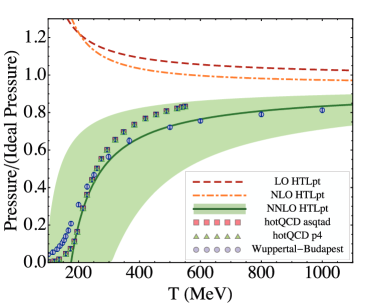
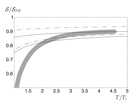
Figure 39: Comparison between the predictions of two versions of HTL–resummed perturbation theory for thermodynamics and the respective lattice results. Left panel: the predictions of HTLpt [118] for the pressure at one–loop (LO), 2–loop (NLO) and, respectively, 3–loop (NNLO) order [111] vs. the lattice results (small cercles, triangles or squares) from two different collaborations. Right panel: the 2–loop result of the ‘2–particle irreducible resummation’ of the entropy [117] — solid and dotted lines correspond to two successive approximations for the thermal masses — vs. the lattice results shown as the grey band. In both cases, a good agreement with the lattice results is observed for temperatures $T\gtrsim 2.5T_{c}$. The theoretical ‘error bands’ follows from varying the renormalization scale in the range $\pi T\leq\mu_{\rm ren}\leq 4\pi T$.

Here $\mu_{\rm ren}$ is the renormalization scale, as introduced by the subtraction of the ultraviolet divergences. In perturbation theory at finite temperature, it is convenient to choose $\mu_{\rm ren}=2\pi T$ as the central value and study the dependence of the results upon variations in $\mu_{\rm ren}$ (typically by a factor of 2) around this central value. These variations measure the stability of the calculations against higher order corrections and thus are indicative of the theoretical uncertainties. They are shown as ‘error bands’ for the theoretical results in Figs. 37 and 39.

 

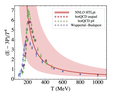
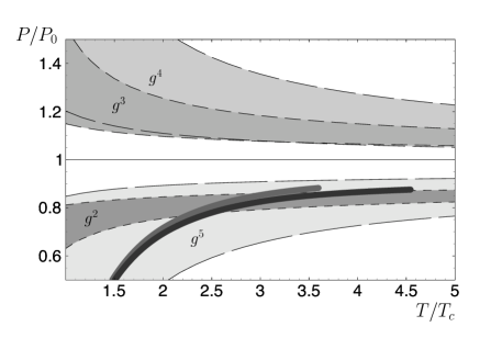
Figure 37: Left panel: the trace anomaly in QCD, as numerically computed on the lattice [107, 108], together with the respective predictions of a ‘HTL–resummed’ perturbation theory [111] (see the text for details), shown as a band (due to the uncertainty in the choice of the renormalization scale $\mu_{\rm ren}$). Right panel: the predictions of (strict) perturbation theory for the pressure, as computed up to order $g^{2}$, $g^{3}$, $g^{4}$, and $g^{5}$, respectively. Whereas the $\mathcal{O}(g^{2})$–result appears to match the lattice results (the dark grey band) rather closely, this agreement is spoilt after including higher order corrections; the ensuing series in powers of $g$ shows no sign of convergence.

The peak in the l.h.s. of fig:trace is a hallmark of the phase transition and is clearly non–perturbative. But for temperatures above $T_{c}$, the ‘trace anomaly’ is rapidly decreasing (its relative strength becomes of order 10% for $T\gtrsim 3T_{c}$), thus suggesting that a perturbative approach may become viable. This is furthermore indicated by the fact that, for $T\gtrsim 3T_{c}$, the pressure and the energy density reach about 80% of the respective values for an ideal gas of quarks and gluons, denoted as ‘SB’ (from ‘Stefan–Boltzmann’) in fig:pressure. A deviation of 20% may seem sufficiently small to be easily accommodated in perturbation theory, but this turns out not to be the case. There are two main reasons for that. First, unlike what happens at $T=0$, where perturbation theory in QCD is an expansion in powers of $\alpha_{s}\equiv g^{2}/4\pi$, at finite temperature this is rather an expansion in powers of $g$, for reasons to be shortly explained. Second, the relevant values of the QCD running coupling are not that small: for $T\simeq 3T_{c}$ and hence $2\pi T\simeq 2$ GeV, one has $\alpha_{s}\simeq 0.25$ and hence $g=1.5\div 2$. For such large valus of $g$, there is no reason why an expansion in powers of $g$ should converge, and indeed it does not: as visible in the right panel of fig:trace, the successive corrections of $\mathcal{O}(g^{2})$, $\mathcal{O}(g^{3})$, $\mathcal{O}(g^{4})$, and $\mathcal{O}(g^{5})$ jump up and down, without any sign of convergence. (The weak–coupling expansion of the pressure in QCD is known to $\mathcal{O}(g^{6}\ln(1/g))$ [112], which is the highest order that can be computed in perturbation theory: the corrections of $\mathcal{O}(g^{6})$ and higher are afflicted with severe infrared divergences due to magnetic gluons; see below.)

The reason why, at finite temperature, perturbation theory is an expansion in powers of $g$ rather than $\alpha_{s}$ is because the quantum corrections associated with soft gluons — those with momenta $k$ much smaller than $T$ — are amplified by the Bose–Einstein thermal distribution function:

$$n_{B}(k)\,=\,\frac{1}{\rme^{\beta E_{k}}-1}\,\simeq\,\frac{T}{E_{k}}\,\gg\,1\quad\mbox{when}\quad E_{k}=|\bm{k}|\,\ll\,T\,.$$ (63)

This property is generic: it holds for any field theory which involves massless bosons (e.g., it holds for photons in a QED plasma). When $k\to 0$, the thermal factors $n_{B}(k)\simeq T/k$ lead to infrared divergences in the calculation of Feynman graphs, which are regulated by plasma effects, like Debye screening. These effects typically enter at the ‘soft’ scale $gT$. For instance, the Debye mass $m_{D}\equiv 1/r_{D}$ which characterizes the exponential screening of the electric colour charge by the plasma constituents, is generated by the one–loop diagrams illustrated in the right panel of fig:debye, which yield $m_{D}\sim gT$. The resummation of these diagrams within the propagator of the exchanged gluon, as also illustrated in fig:debye, renders the (electric) gluons effectively massive : $E_{k}=\sqrt{k^{2}+m_{D}^{2}}$. Hence, when $k\to 0$, the Bose–Einstein occupation number remains finite, but it is parametrically large: $n_{B}(k)\simeq T/m_{D}\sim 1/g$. This inverse power of $g$ changes the perturbative order of the 2–loop correction to the pressure with one ‘hard’ loop ($k\sim T$) and one ‘soft’ ($k\lesssim gT$) from $\alpha_{s}^{2}\sim g^{4}$ to $g^{4}n_{B}(k)\sim g^{3}$. This is the origin of the odd powers of $g$ in the perturbative expansion.

One should also mention here that Debye screening, as illustrated in the left panel of fig:debye, is operational for the electric gluons (i.e. for the Coulomb interactions), but not also for the magnetic ones — those having transverse polarizations. For non–relativistic plasmas, magnetic interactions are suppressed by powers of the velocities, but for (ultra)relativistic plasmas, like the QGP, they are as important as the electric ones. One expects magnetic interactions in the QGP to be screened at the ‘ultrasoft’ scale $m_{\rm mag}\sim g^{2}T$, but the associated physics — in particular, the contribution of the ‘ultrasoft’ magnetic gluons to thermodynamics, which starts at $\mathcal{O}(g^{6})$ — cannot be computed in perturbation theory. Indeed, each additional ‘ultrasoft’ loop is accompanied by a factor $\sim g^{2}n_{B}(k)\sim g^{2}(T/m_{\rm mag})\sim 1$, meaning that diagrams with arbitrarily many such loops contribute at the same order in $g$. This explains why the corrections of $\mathcal{O}(g^{6})$ are non–perturbative, as alluded to above.

In QCD, the Debye mass is only one example of a class of one–loop ‘corrections’ which are non–perturbative at the ‘soft’ scale $gT$ and should be viewed as a part of the leading–order theory at that scale, and not as corrections [116, 113]. These diagrams are known as hard thermal loops, since the typical momenta within the loop are of order $T$ (the value preferred by the statistical, Bose–Einstein and Fermi–Dirac factors) and thus are hard compared to the soft ($k\sim gT$) momenta flowing along the external legs. There are HTL’s with any number $n$ of external gluons lines and with either zero, or two, quark external lines (see fig:HTL for some examples). They are generally non–local, that is, they depend upon the external, soft, momenta. In particular, the HTL’s for the 2–point functions (the quark and gluon self–energies) encode phenomena like Debye screening for the electric gluons, dynamical screening (or Landau damping) for the magnetic gluons, and the dispersion relations for on–shell quanta with momenta of order $gT$. Such quanta have wavelengths $\lambda\sim 1/gT$ which are parametrically larger than the typical separation $\sim 1/T$ between the typical plasma constituents — quarks and gluons with momenta of order $T$. Accordingly, the soft modes are truly collective excitations (or ‘plasma waves’), with either quark or gluon quantum numbers.

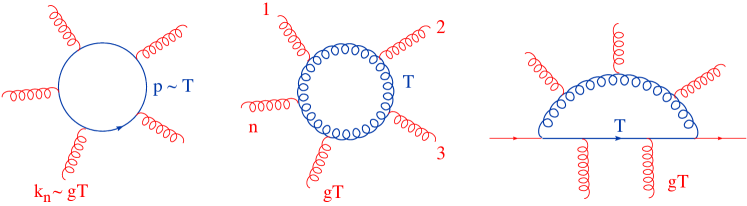
Figure 38: A few examples of hard thermal loops (HTL’s). All the external momenta are soft ($k_{i}\sim gT$) and the loop integrations are dominated by relatively hard modes with $p\sim T$.

As already mentioned, the HTL’s are of the same order as the respective tree–level amplitudes with ‘soft’ external legs, so they cannot be expanded out in perturbation theory. Rather, one needs to perform a reorganization of the perturbation theory in which the HTL’s are viewed as a part of the leading–order theory for the soft modes. Roughly speaking, this amounts to expanding around a gas of dressed quasi–particles whose zeroth–order properties (propagators and interaction vertices) are encoded in the HTL’s. In practice, there are various ways to perform such reorganizations and it is quite reassuring that all the methods that have been proposed so far [117, 114, 115, 118, 111, 112] appear to be successful in describing the lattice data (although with considerably different amounts of efforts).

One of these methods, known as ‘HTL perturbation theory’ (HTLpt) [118], consists in including the HTL’s in the ‘tree–level’ effective theory, by adding and subtracting $\mathcal{L}_{\rm HTL}$ (the sum of the HTL amplitudes) to/from the original Lagrangian:

$$\mathcal{L}_{\rm QCD}=\mathcal{L}_{0}+\mathcal{L}_{\rm int}=\big{(}\mathcal{L}_{0}+\mathcal{L}_{\rm HTL}\big{)}+\big{(}-\mathcal{L}_{\rm HTL}+\mathcal{L}_{\rm int}\big{)}=\mathcal{L}^{\prime}_{0}+\mathcal{L}_{\rm int}^{\prime}\,.$$ (64)

In this equation, $\mathcal{L}_{0}$ is the free ($g=0$) piece of the QCD Lagrangian, $\mathcal{L}_{\rm int}$ is the respective interaction piece, $\mathcal{L}^{\prime}_{0}\equiv\mathcal{L}_{0}+\mathcal{L}_{\rm HTL}$ represents the new ‘tree–level Lagrangian’ which defines the Feynman rules (HTL–resummed propagators and vertices) of HTLpt, and, finally, $\mathcal{L}_{\rm int}^{\prime}\equiv\mathcal{L}_{\rm int}-\mathcal{L}_{\rm HTL}$ is the new ‘interaction Lagrangian’. The subtracted piece $-\mathcal{L}_{\rm HTL}$ within $\mathcal{L}_{\rm int}^{\prime}$ acts as a ‘counterterm’ to prevent double counting (the HTL’s have been already included in the zeroth–order theory and they should not be regenerated via loop corrections in HTLpt) and also to correct for the fact that, within $\mathcal{L}^{\prime}_{0}$, the HTL’s are used for all the modes, including the hard modes to which they do not really apply (this introduces spurious contributions at lower orders which are compensated by the ‘counterterm’ only in higher orders). In order for such compensations to efficiently work, one needs to go up to relatively high orders in HTLpt, which involve very tedious calculations (due to the non–local nature of the HTL’s). It was only recently, after pushing such calculations up to three loop order [111], that one has finally reached a good agreement with the respective lattice results for $T\gtrsim 2.5T_{c}$. This agreement is visible in the left panel of fig:trace for the trace anomaly and in the left panel of fig:resum for the pressure.

A more economical approach, in which a similarly good agreement with the lattice results (see the right panel of fig:resum) has been obtained via a simpler, 2–loop, calculation, is the ‘2–particle irreducible (2PI) resummation’ of the entropy [117, 114]. In that approach, most of the difference between the 2PI result for $S$ and the corresponding result $S_{SB}$ for the ideal gas comes from the thermal masses $m_{q},\,m_{g}\sim gT$ acquired by the hard ($k\sim T$) quarks and gluons via interactions in the plasma. Albeit formally small ($m_{q,g}\sim gT\ll k\sim T$), these masses cannot be expanded in perturbation theory, since such an expansion would generate powers of $m^{2}/k^{2}$ leading to infrared divergences in the integral over $k$. The success of the 2PI description supports the physical picture of the QGP in terms of quasi–particles — quarks and gluons with typical momenta $k\sim T$, which are dressed by the medium (in particular, in the sense of acquiring thermal masses), but whose residual interactions are relatively small. Moreover, a substantial part of these residual interactions can be associated with collective excitations and screening effects at the ‘soft’ scale $gT$, as encoded in the HTL–resummed propagators.

 

It is furthermore interesting to notice that the HTL resummation is based on the separation of scales $gT\ll T$ which is a priori valid at weak coupling ($g\ll 1$), yet this turns out to rather successfully describe the lattice data in a temperature range where $g=1.5\div 2$. This confirms that the failure of ordinary perturbation theory (cf. fig:trace, right panel) is not imputable to the fact that the coupling is relatively strong, but rather it is a consequence of expanding out the medium effects in powers of $g$ in a kinematical domain where they are truly non–perturbative.

Yet, the issue of the strength of the coupling remains open in so far as the study of dynamical phenomena is concerned. These phenomena refer to non–trivial evolutions in time, say off–equilibrium deviations in response to external perturbations. As long as the perturbations are small, their effects can be computed within the linear response theory, via the Kubo formula: the response of the plasma is linear in the strength of the perturbation, with a proportionality, or ‘transport’, coefficient which represents a correlation function in thermal equilibrium. For instance, a constant electric field ${\bf E}$ acting on the quark constituents of the plasma (which carry electric charge) induces an electromagnetic current with density $\langle j^{i}_{\rm em}\rangle=\sigma E^{i}$, where $\sigma$ is the electrical conductivity. The respective Kubo formula relates $\sigma$ to the long–wavelength ($k^{i}\to 0$) and zero–frequency ($\omega\to 0$) limit of the current–current correlator in thermal equilibrium. Other transport coefficients include the (quark) flavor diffusion coefficients and the shear viscosity $\eta$ introduced in shear. The use of Kubo formulæ for perturbative calculations at weak coupling turns out to be quite tedious, because of the need to perform sophisticated resummations [119]. However, these formulæ are very useful for non–perturbative calculations of the transport coefficients, either on the lattice [100], or via the AdS/CFT correspondence at strong coupling [120].

For a weakly coupled QGP and to leading order in the coupling, the transport coefficient can be alternatively, and more efficiently, computed from the Boltzmann equation (linearized with respect to the off–equilibrium perturbation). This amounts to solving a linear integral equation which effectively resums an infinite number of diagrams of the ordinary perturbation theory in thermal equilibrium. These diagrams describe multiple scattering via soft gluon exchanges and can be generated by iterating the $2\to 2$ elastic processes shown in fig:elastic arbitrarily many times. The ensuing transport coefficients are of the parametric form anticipated (on the example of the shear viscosity) in shearQGP, but the use of the Boltzmann equation allows one to obtain more precise results, which are complete to leading order in $\alpha_{s}$ [121, 122]. Yet, these results are deceiving with respect to the heavy–ion phenomenology: as already mentioned in sec:hydro, the leading order estimate for $\eta/s$ is too large to be consistent with the hydrodynamical description of the data.

The last observation raises the question of the next–to–leading order corrections. Their calculation is extremely complicated and so far this has been accomplished for just one quantity: the diffusion coefficient $D$ for a heavy quark with mass $M\gg T$. In the context of HIC, this quantity controls the collisional energy loss and the thermalization of heavy quarks like the charm or the bottom. Once again, the LO perturbative estimate for $D$ [123] appears to be too large to be consistent with the data. The NLO correction to $D$ is of relative order $g$ and has been computed in Ref. [124]. This appears to go in the right direction (it diminishes the value of $D$), but the effect is extremely large for realistic values of $g$ — the NLO ‘correction’ is almost an order of magnitude larger than the respective LO result ! —, thus rising doubts about the reliability of the whole scheme. It looks like the perturbative series suffers from a lack–of–convergence problem similar to that noticed for the pressure. It might be that this problem too will be cured by all–orders resummations of the HTL’s; but this issue is still open since such resummations have not yet been performed for dynamical quantities. Alternatively, there is the possibility that the transport phenomena, which involve long–range dynamics, be sensitive to rather large values of the QCD running coupling, which exclude weak–coupling techniques. If so, one could search for physical guidance in the corresponding results at strong coupling, as obtained via the AdS/CFT correspondence (see sec:AdS below). Finally, let us notice that the first lattice results for the transport coefficients have started to emerge, although the current errors bars are still quite large. These calculations are very difficult as they require to numerically perform an analytic continuation (from imaginary time to real time), which in turns requires very precise numerical data. In view of that, it is quite encouraging that the recent lattice results for the heavy quark diffusion coefficient [125, 126] appear to be consistent with the heavy–ion phenomenology, within the (lattice and experimental) errors bars.

4.4 Jet quenching

In sec:pA we have mentioned two interesting phenomena occurring in ‘dense–dilute’ (p+A or d+A) collisions — the suppression of particle production and that of azimuthal di–hadron correlations at forward rapidities —, which in that context have been interpreted as consequences of gluon saturation in the wavefunction of the nuclear target: the larger the rapidity, the smaller the values of the longitudinal momentum fraction that are probed in the nucleus, and hence the stronger the saturation effects. On the other hand, the RHIC data for d+Au collisions at central rapidities ($\eta\leq 1$) show no similar suppression (see the 2 left-most plots in fig:dAu and also the corresponding data in the right plot in fig:azimuthal below), which implies that nuclear saturation effects are not important in the central–rapidity kinematics at RHIC. (But this is likely to change at the LHC; see e.g. [14, 127, 69].) The situation is however different for the ‘dense–dense’ A+A collisions: the respective data at RHIC and the LHC show a strong suppression of particle production and of the azimuthal di–hadron correlations already for central rapidities (and for relatively hard transverse momenta). These phenomena cannot be related to ‘initial–state’, saturation, effects in the incoming nuclei (at least not fully), since they do not show up in the mid–rapidity d+Au data at RHIC. Rather, they must correspond to interactions in the final state, that is, interactions with the dense partonic medium (the glasma and the quark–gluon plasma) which exists at intermediate stages. The change in the properties of a hard particle or of the associated jet induced by its interactions in the medium is generally referred to as jet quenching (see e.g. [128, 129, 130, 131] for recent reviews).

  

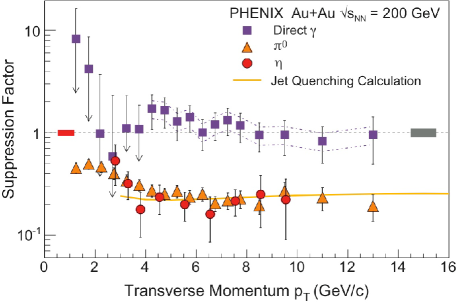
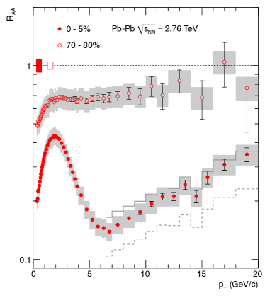
Figure 40: The nuclear modification factor $R_{AA}$, as measured in central Au+Au collisions at RHIC (PHENIX, left panel) and in Pb+Pb collisions at the LHC (CMS, right panel). For comparaison, one also shows the data for the production of direct photons, which show no nuclear effect as expected (left panel) and for hadron production in peripheral collisions, for which the nuclear effects are quite small (right panel).

The suppression of particle production in A+A collisions is best characterized by the ratio $R_{AA}$ (the ‘nuclear modification factor’), defined by analogy with RpA, that is

$$R_{AA}(\eta,p_{\perp})\,\equiv\,\frac{1}{N_{coll}}\,\frac{\frac{\rmd N_{h}}{\rmd^{2}p_{\perp}\rmd\eta}\Big{|}_{AA}}{\frac{\rmd N_{h}}{\rmd^{2}p_{\perp}\rmd\eta}\Big{|}_{pp}}\,,$$ (65)

where the number $N_{coll}$ of binary collisions at a given impact parameter scales like $A^{4/3}$ (for relatively central collisions): indeed, there is a factor $A^{1/3}$ associated with the longitudinal width of each of the two nuclei and an additional factor of $R_{A}^{2}\propto A^{2/3}$ coming from the integral over all the impact parameters. The experimental results for $R_{AA}$ (at mid–rapidities) in Au+Au collisions at RHIC ($\sqrt{s_{NN}}=200$ GeV) and in Pb+Pb collisions at the LHC ($\sqrt{s_{NN}}=2.76$ TeV) are shown in the left and right panels of fig:RAA, respectively. As anticipated, they show a substantial suppression of the hadron production as compared to p+p collisions, which persists up to $p_{\perp}\simeq 20$ GeV, at least. The interpretation of this suppression as a dense–medium effect is furthermore supported by the fact that (i) the direct photons (which do not interact with the hadronic matter) show indeed no suppression (cf. the left figure), and (ii) even for hadrons, the suppression is considerably smaller in the peripheral collisions (cf. the right figure), in agreement with the fact that the density and the size of the produced medium are much smaller in that setup. Note also that the suppression at intermediate values $p_{\perp}\simeq 6\div 7$ GeV is stronger at the LHC than at RHIC, indicating that the medium produced there is denser, as expected.

  

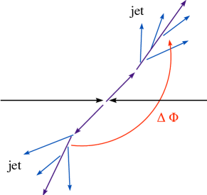
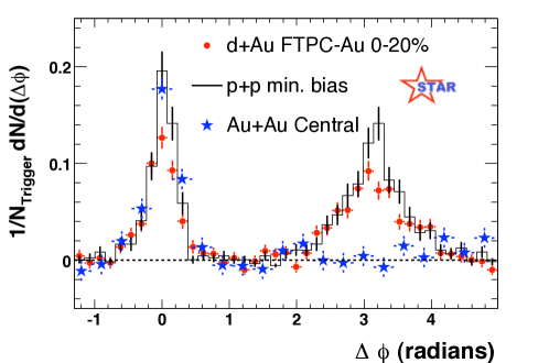
Figure 41: Left: cartoon of a typical di–jet event as produced by a hard scattering. Right: azimuthal distribution of hadrons with $p_{\perp}\geq 2$ GeV relative to a trigger hadron with $p_{\perp}\geq 4$ GeV, as measured at RHIC (STAR), in p+p, d+Au and central Au+Au collisions [132].

Concerning the suppression of azimuthal correlations in the di–hadron production, this is clearly visible in the right plot in fig:azimuthal, which shows data taken at RHIC for hadrons with $p_{\perp}\gtrsim 2$ GeV : unlike for p+p and d+Au collisions, where one can see a peak at $\Delta\Phi=\pi$, as expected for a pair of hadrons which are produced back–to–back, there is no such a peak in the central Au+Au collisions. This is interpreted as the consequence of the interactions suffered by the ‘away’ particle (the one that would have normally emerged at $\Delta\Phi=\pi$) while propagating through the medium. Via such interactions, the particle transverse momentum has been degraded and/or the particle has been deviated towards different directions, so it will not show up around $\Delta\Phi=\pi$, nor in the original bin in $p_{\perp}$.

 

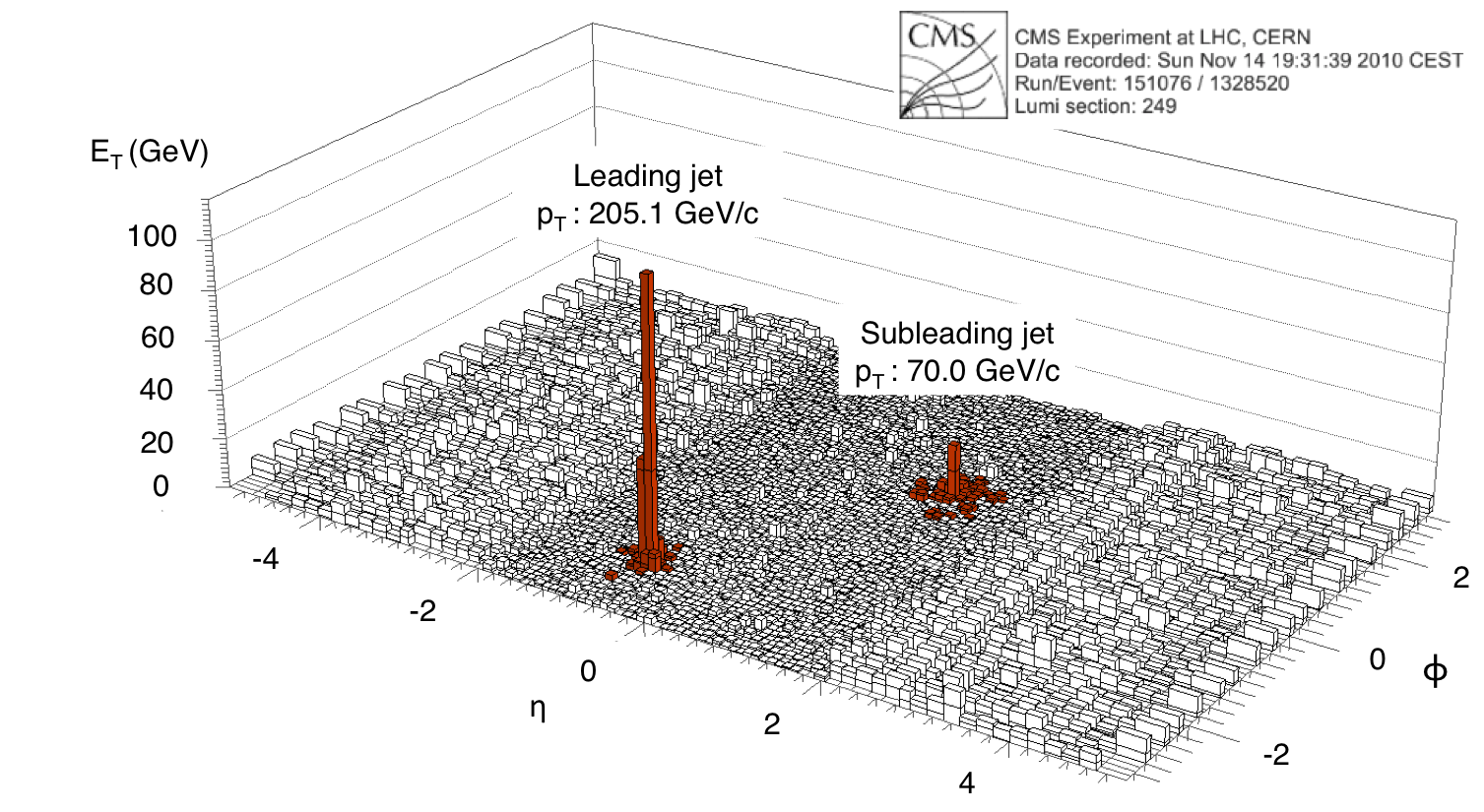
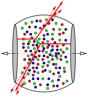
Figure 42: Left panel: a highly asymmetric di–jet event in Pb+Pb collisions at the LHC as measured by CMS. Right panel: a cartoon of an asymmetric di–jet event in A+A collisions. The hard scattering producing the jets occurs near the edge of the fireball. One of the jets (the ‘trigger jet’) leaves the medium soon after its formation and thus escapes unscattered, while the other one (the ‘away jet’) crosses the medium and is strongly modified by the latter.

Besides confirming and sharpening the discoveries at RHIC, the first heavy ion data at the LHC revealed a new phenomenon, whose observation was possible because of the unprecedented ability of the detectors there (notably the calorimeters at ATLAS and CMS, with a wide coverage in rapidity) to reconstruct jets: the di–jet asymmetry [133, 134]. Namely, a significant fraction of the di–jet events in Pb+Pb collisions at $\sqrt{s_{NN}}=2.76$ TeV shows a large transverse energy imbalance between the trigger (or ‘leading’) jet and the away (or ‘subleading’) jet. (The left panel in fig:dijets and the right panel in fig:events display such asymmetric di–jet events, as measured by CMS.) One should stress that the criterion used to define a ‘jet’ — the value of the product $R=\Delta\Phi\times\Delta\eta$ between the spreadings of the hadron yield in azimuthal angle and in pseudo–rapidity — is the same for the leading and subleading jets. Moreover, a substantial asymmetry between the two jets exists already in p+p collisions, because of the bias introduced by the trigger process (see the histograms in fig:AJ). But the heavy ion collisions show a significant increase in this asymmetry, which becomes more pronounced with increasing centrality. A quantitative way to characterize this asymmetry is via the transverse energy imbalance,

$$A_{\rm J}=\frac{p_{\perp 1}-p_{\perp 2}}{p_{\perp 1}+p_{\perp 2}}\,,$$ (66)

where $p_{\perp 1}$ ($p_{\perp 2}$) is the transverse momentum of the leading (subleading) jet. The normalization in AJ is useful for removing uncertainties in the overall jet energy scale. fig:AJ (left panel) shows the distribution of the Pb+Pb events as a function of $A_{\rm J}$, in different bins of centrality: for the most peripheral collisions, this is quite similar to the respective distribution for p+p collisions, as shown in figure (a). But for the more central collisions, there is an increase in the fraction of events with relatively large $A_{\rm J}=0.3\div 0.4$, which significantly exceeds the respective prediction of the PYTHIA Monte–Carlo event generator (which neglects the medium effects). This demonstrates that there is additional energy loss by the jet, estimated as 20 to 30 GeV, due to its interactions in the medium. But this energy loss does not lead to significant angular decorrelations: as visible in the right panel of fig:AJ, the distribution of the subleading jet is still peaked at $\Delta\Phi_{12}=\pi$, like in p+p collisions (and in good agreement with the PYTHIA simulations). This implies that the additional energy loss is not to be attributed to rare, hard, emissions (which would typically lead to 3–jet events). A careful analysis of the background around the away side jet allowed one to establish that the missing energy is in fact associated with relatively soft particles ($p_{\perp}\leq 2$ GeV) emitted at large angles with respect to the jet axis [134]. This rises the question about the physical mechanism which is responsible for such in–medium emissions at large angles.

 

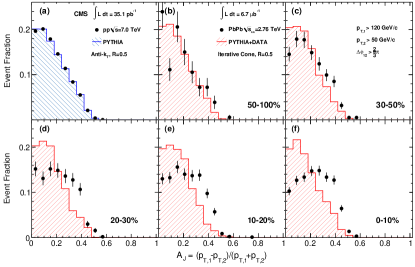
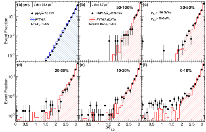
Figure 43: The distribution of the CMS data for p+p collisions ($\sqrt{s}=7$ GeV) and Pb+Pb collisions ($\sqrt{s_{NN}}=2.76$ TeV) as a function of $A_{\rm J}$ (left panel) and respectively of the azimuthal separation $\Delta\Phi_{12}$ w.r.t. the leading–jet axis (right panel) in different bins of centrality: (a) refers to p+p, (f) to the 10% most central Pb+Pb, (e) to the centrality bin 10-20%, etc. The histograms show the respective predictions of PYTHIA, which agree well with the data for p+p and for peripheral Pb+Pb, but not also for central Pb+Pb. From Ref. [134].

As we shall now explain, a natural mechanism in that sense exists in QCD at weak coupling: this is medium–induced gluon radiation, that is, the emission of gluons stimulated by the interactions between the partons composing the jet and the constituents of the medium. The most interesting situation — originally studied by Baier, Dokshitzer, Mueller, Peigné, and Schiff [135, 136] and independently by Zakharov [137, 138], following pioneering work by Gyulassy and Wang [139] (see also [140, 141, 142, 143, 144, 145, 146]) —, is when the medium is so dense that the gluon formation time is much larger than the mean free path of a parton propagating through the medium. In that case, there are many collisions which coherently contribute to the emission of a single gluon (see fig:BDMPS), leading to a suppression of the radiation spectrum as compared to the (Bethe–Heitler) spectrum that would be produced via independent multiple scattering. This suppression is known as the Landau–Pomeranchuk–Migdal (LPM) effect.

The ‘gluon formation time’ is the typical time that it takes in order to emit a gluon with a given kinematics. This concept is quite similar to the ‘fluctuation lifetime’ introduced in lifetime, but it is instructive to present here an alternative derivation for it, which is adapted to the problem at hand. To be specific, consider the emission of a gluon with momentum $\bm{k}$ and energy $\omega=|\bm{k}|$ by an energetic quark propagating along the $z$ axis. Even though the $q\bar{q}g$ vertex in QCD is local, the emission process is truly non–local, as it takes some time for the emitted gluon to lose coherence w.r.t. its parent quark. Namely, when the gluon starts being emitted, its wavefunction is still overlapping with that of the quark, so the two quanta cannot be distinguished from each other. But with increasing time, the gluon separates from the quark and their quantum coherence gets progressively lost. When the quark is very energetic, the gluon is typically emitted at a very small angle $\theta\simeq k_{\perp}/\omega\ll 1$ and the coherence between the two quanta is measured by their overlap in the transverse space. The gluon is considered as being ‘formed’ (or ‘fully emitted’) when its transverse separation $b_{\perp}\simeq\theta\Delta t$ from the quark becomes larger than its transverse Compton wavelength $\lambda_{\perp}=1/k_{\perp}\simeq 1/(\omega\theta)$. This condition is satisfied after a time

$$\Delta t_{\rm form}\,\simeq\,\frac{2\omega}{k_{\perp}^{2}}\,\simeq\,\frac{2}{\omega\theta^{2}}\,.$$ (67)

(The factor of 2 in the numerator is conventional.) The above argument is completely general: it holds for gluon emissions in the medium or in the vacuum. What is different, however, in the two cases is the mechanism causing the radiation and the associated gluon spectrum.

To better appreciate this difference, remember first that an on–shell quark cannot radiate: it can produce virtual fluctuations and thus develop a partonic substructure, as discussed in sec:CGC, but energy–momentum conservation prevent these quanta to become on–shell, and hence to separate from the parent quark. For the radiation to be possible, the quark and/or the emitted gluon must suffer additional interactions, which provide the energy deficit.

Consider first the situation in the vacuum : the quark is produced in an off–shell state via a hard scattering and then evacuates its virtuality via bremsstrahlung. Namely, it emits a gluon with energy $\omega$ and transverse momentum $k_{\perp}$ within a time interval $\Delta t\sim{2\omega}/k_{\perp}^{2}$ after the original scattering. These values $\omega$ and $k_{\perp}$ are arbitrary (subjected to energy–momentum conservation) and independent of each other. However the bremsstrahlung spectrum, brem, favors the emission of soft ($x\ll 1$, or relatively small $\omega$) and nearly collinear ($\theta\to 0$, or small $k_{\perp}$) gluons, for which the formation time is long.

  

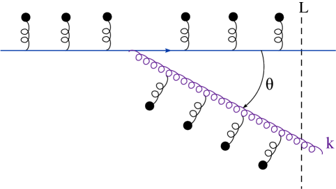
Figure 44: Right: A cartoon illustrating medium–induced gluon radiation by an energetic quark propagating through a dense QCD medium. Both the quark and the emitted gluon undergo multiple scattering off the medium constituents (represented by the black blobs). Left: A quark-antiquark antenna emitting a gluon (here, from the antiquark leg) within the medium with size $L$. The interactions with the medium are not explicitly shown.

The situation is very different for a quark propagating through a dense medium : the quark undergoes collisions with the medium constituents, with a typical distance $\ell$ (the mean free path) between two successive collisions. Any such a collision provides a small acceleration, thus allowing the quark to radiate. Accordingly, the initial virtuality of the quark is not essential anymore: the quark can now radiate anywhere within the medium, and not only within a distance $\sim\Delta t_{\rm form}$ after the original hard scattering. This implies that the phase–space for in–medium emissions is enhanced by a factor $L/\Delta t_{\rm form}$ with respect to emissions in the vacuum. Here $L$ is the longitudinal extent of the medium as crossed by the quark and is typically much larger than $\Delta t_{\rm form}$, as we shall see. Moreover, the emission mechanism and the associated formation time are influenced by the gluon interactions in the medium, which destroy the coherence between the gluon and the parent quark and thus facilitate the radiation.

To estimate $\Delta t_{\rm form}$ for medium–induced emissions, we also need the rate at which the (virtual) gluon accumulates transverse momentum via rescattering in the medium. We shall later check that the successive collisions proceed independently from each other and thus provide transverse momenta which are randomly oriented and add in quadrature. This implies that the average transverse momentum squared grows linearly with time: $\langle k_{\perp}^{2}\rangle\simeq\hat{q}\Delta t$, where $\Delta t$ is the lifetime of the virtual gluon, as measured from the emission vertex, and $\hat{q}$ is a medium–dependent transport coefficient known as the jet quenching parameter, to be specified later. Hence, during its formation, the gluon acquires a typical transverse momentum squared $k_{f}^{2}\simeq\hat{q}\Delta t_{\rm form}$ via scattering within the medium. On the other hand, the condition for quantum decoherence requires the relation tau between $\Delta t_{\rm form}$ and $k_{f}^{2}$. Together, these two conditions determine both the formation time and the typical transverse momentum of the gluon at the time of emission:

$$\Delta t_{\rm form}\,\simeq\,\frac{2\omega}{k_{f}^{2}}\quad\&\quad k_{f}^{2}\simeq\hat{q}\Delta t_{\rm form}\quad\Longrightarrow\quad\Delta t_{\rm form}\,\simeq\,\sqrt{\frac{2\omega}{\hat{q}}}\quad\&\quad k_{f}^{2}\,\simeq\,(2\omega\hat{q})^{1/2}\,.$$ (68)

We thus see that, for medium–induced radiation, $k_{\perp}$ and $\omega$ are not independent kinematical variables anymore: the transverse momentum of the emitted gluon is acquired via interactions in the medium during the formation time which grows with the energy like $\Delta t_{\rm form}\propto\omega^{1/2}$.

This mechanism for gluon production is operational provided the formation time is much larger than the mean free path $\ell$, but smaller than the size $L$ of the medium which is available for the emission process (the distance traveled through the plasma by the parent quark):

$$\ell\,\ll\,\Delta t_{\rm form}\,\leq\,L\quad\Longrightarrow\quad\omega_{\rm min}\,\equiv\,\frac{1}{2}\,\hat{q}\,\ell^{2}\,\ll\,\omega\,\leq\,\omega_{c}\,\equiv\,\frac{1}{2}\,\hat{q}L^{2}\,.$$ (69)

These arguments imply that the typical emission angle at the time of formation, $\theta_{f}\simeq{k_{f}}/{\omega}$, cannot be arbitrarily small:

$$\theta_{f}\,\simeq\,\frac{k_{f}}{\omega}\,\simeq\,\left(\frac{2\hat{q}}{\omega^{3}}\right)^{1/4}\quad\Longrightarrow\quad\theta_{c}\,\equiv\,\frac{2}{\sqrt{\hat{q}L^{3}}}\,\leq\,\theta_{f}\,\ll\,\theta_{\rm max}\,\equiv\,\frac{2}{\sqrt{\hat{q}\ell^{3}}}\,.$$ (70)

Unlike bremsstrahlung, the in–medium radiation does not favour collinear radiation. In fact, the smaller is the gluon energy $\omega$, the larger is the emission angle $\theta_{f}$ and the shorter the emission time $\Delta t_{\rm form}$. The final spectrum favors indeed the emission of relatively soft gluons with $\omega\ll\omega_{c}$, for which the formation time is much smaller than the size of the medium, $\Delta t_{\rm form}\ll L$, and the emission angle is quite large: $\theta_{f}\gg\theta_{c}$. Moreover, after being emitted, the gluons keep interacting with the medium and thus get deflected at even larger angles: their average transverse momentum can rise up to a final value $\langle k_{\perp}^{2}\rangle\simeq\hat{q}(L-t_{0})\sim\hat{q}L$, where $t_{0}$ is the time at the emission vertex. This phenomenon is known as transverse momentum broadening.

The above considerations show that the medium–induced radiation is very efficient in broadening the jet energy in the transverse plane, via the emission of soft ($\omega\ll\omega_{c}$) gluons, in qualitative agreement with the LHC data for di–jet asymmetry. On the other hand, the $R_{AA}$ data for ‘high–$p_{\perp}$ suppression’ are probably more sensitive to the emission of harder gluons, with $\omega\sim\omega_{c}$, which dominate the energy loss by the ‘leading particle’ (the parton which has initiated the jet). Accordingly, the total energy loss $\Delta E\sim\omega_{c}\sim\hat{q}L^{2}$ scales like the square of the medium length $L$, and not like $L$ (as one would expect for a mechanism where the energy is lost locally, say via elastic collisions in the medium). The reason for this scaling with $L^{2}$ is, of course, the fact that the actual mechanism at work is non–local : it takes a time $\Delta t_{\rm form}(\omega)$ to emit a gluon and for $\omega\sim\omega_{c}$ this time is of the order of $L$. Since moreover the emission can be initiated at any point within $L$, the overall energy loss scales like $L^{2}$. Reversing the argument, one concludes that the stopping length for a particle which loses all its energy inside the medium scales like $L_{\rm stop}\sim E^{1/2}$, where $E$ is the initial energy of that particle.

For more quantitative studies and applications to phenomenology, one still needs an estimate for the jet quenching parameter $\hat{q}$. Let us assume, for definiteness, that the medium is a quark–gluon plasma with (local) temperature $T$ and weak coupling. The typical collisions which matter for the problem at hand are soft, in the sense that the typical transferred momentum is of the order of the Debye mass $m_{D}\sim gT$ introduced in sec:QGP. This is so since the soft collisions occur much more frequently than the hard ones: the corresponding cross–section is not the transport cross–section evaluated in sigma (that was the cross–section for scattering at large angles), but rather the total cross–section

$$\sigma_{\rm tot}\,=\,\int\rmd\Omega\,\frac{\rmd\sigma}{\rmd\Omega}\,\propto\,\int\rmd\theta\,\sin\theta\,\frac{\alpha_{s}^{2}}{T^{2}\sin^{4}\theta}\,\sim\,\frac{\alpha_{s}^{2}}{T^{2}}\int_{g}\frac{\rmd\theta}{\theta^{3}}\,\sim\,\frac{\alpha_{s}}{T^{2}}\,\ln\frac{1}{\alpha_{s}}\,.$$ (71)

This is dominated by small–angle scattering — the integral over $\theta$ is cut off at $\theta\sim g$ by the plasma effects — and is larger by a factor $1/\alpha_{s}$ than the transport cross–section sigma. The relevant mean free path is obtained by inserting the total cross–section in mfp : $\ell\sim 1/(n\sigma_{\rm tot})\sim[T\alpha_{s}\ln({1}/{\alpha_{s}})]^{-1}$. As anticipated, this is parametrically larger than the interaction range $1/m_{D}\sim 1/gT$, meaning that successive collisions can be treated as independent. Since on the average there is a transfer $\Delta k_{\perp}^{2}\sim m_{D}^{2}$ of transverse momentum squared per collision, we finally conclude that

$$\hat{q}\,\equiv\,\frac{\rmd\langle k_{\perp}^{2}\rangle}{\rmd t}\,\simeq\,\frac{m_{D}^{2}}{\ell}\,\sim\,\alpha_{s}^{2}T^{3}\ln({1}/{\alpha_{s}})\,,$$ (72)

for a weakly–coupled QGP. This is merely a parametric estimate, valid to leading logarithmic accuracy, and as such it suffers from the same lack–of–accuracy drawback as discussed for other transport coefficients towards the end of sec:thermo: it cannot be trusted for phenomenological applications. In fact, the whole set–up above described is a bit too idealized to correspond to the actual experimental situation. To cope with that, more sophisticated, phenomenological models have been proposed which treat the geometry of the collision in a more realistic way (finite volume, longitudinal expansion, time and point dependent jet quenching parameter) and include also free parameters. Such models are quite successful in describing the data, for both the $R_{AA}$ ratio RAA and the di–jet asymmetry AJ (see [147] for a recent discussion and more references), but at the expense of using a rather large (average) value for $\hat{q}$ — considerably larger than the corresponding perturbative estimate to leading logarithmic accuracy. This situation is sometimes viewed as an argument in favor of the strong coupling scenario, but it might simply reflect the inaccuracy of the current perturbative results.

Note finally that the theory discussed above has addressed the (medium–induced) emission of a single gluon, whereas in reality one expects the in–medium evolution of a jet to involve several successive emissions — both by the hard parton which has initiated the jet and by its descendants. (Multiple emissions become important when the quantity $\alpha_{s}(L/\Delta t_{\rm form})$ — which is roughly the probability for one gluon emission — becomes of order one.) Phenomenological models generally assume that successive emissions proceed independently from each other, but this is still to be demonstrated: a priori, there could be interference effects between emissions by different sources (the various partons forming the jet). For jet evolution in the vacuum, one knows that such interference effects are indeed important: they lead to angular ordering of the subsequent emissions — the successive emission angles are smaller and smaller [148, 2]. For the case of in–medium radiation, there is so far no explicit calculation of two (or more) successive emissions, but there are studies of interference effects in the emission by two sources: a quark and an antiquark forming a ‘colour antenna’ (see the right panel of fig:BDMPS) [149, 150, 146]. In particular, the analysis in [146] shows that the interference effects are negligible so long as the antenna opening angle (the angle $\theta_{q\bar{q}}$ in fig:BDMPS) is much larger than the minimal angle $\theta_{c}$ introduced in thetaf. As previously explained, the typical emission angles obey this condition already at the time of formation and they become even larger at later times, due to the momentum broadening by the medium. This suggests that successive medium–induced gluon emissions can be effectively treated as independent, thus justifying a probabilistic approach to in–medium jet evolution, like in Refs. [151, 152, 153].

4.5 The AdS/CFT correspondence: insights at strong coupling

At several points in the previous presentation, we pointed out observables whose values as extracted from the heavy–ion data seem difficult to understand if the coupling is weak, but would be more naturally accommodated at strong coupling. These observables include the viscosity-over-entropy ratio $\eta/s$, the thermalization time $\tau_{\rm eq}$, the jet quenching parameter $\hat{q}$, and the heavy quark diffusion coefficient $D$. In all these cases, the hypothesis of a strong coupling must be subjected to caution. First, these quantities are measured only indirectly, that is, they are extracted from fits to the data based on complex analyses which involve theoretical prejudices (notably, on the overall physics scenario), various assumptions which are difficult to check, and a considerable amount of model–building (concerning e.g. the initial conditions for hydrodynamics, the geometry of the collision, the theoretical description of multi–particle interactions). So, it is fair to say that the systematic uncertainties on these observables are still quite large (even though, within a given scenario, they might be strongly constrained by the data). Second, the weak–coupling results which serve as benchmarks for comparison are generally leading–order results in the perturbative expansion. But, as emphasized in sec:thermo, the standard perturbation theory (i.e. the strict expansion in powers of the coupling) is not reliable for the description of transport phenomena, even if the coupling is weak. This is so because of the need to resum finite–density effects like the Hard Thermal Loops to all orders, and this has not been done so far for dynamical quantities. The situation becomes even more complicated for the far–from–equilibrium situations, as relevant for the phenomenology, where the medium effects are not well understood.

This being said, the hypothesis of a strong coupling is both interesting and intriguing, and not easy to refute on the basis of asymptotic freedom or of the current lattice data. Indeed, as already noted in sec:thermo, the QCD coupling $g$ is quite large when evaluated for temperatures a few times $T_{c}$ (the critical temperature for deconfinement): $g=1.5\div 2$. As also mentioned there, the perturbative series at finite temperature is truly an expansion in powers of $g$ (and not of $\alpha_{s}=g^{2}/4\pi$), so for that purpose the coupling is moderately strong. Reorganizing the perturbation theory via appropriate resummations of medium effects is one of the possible strategies to cope with this problem. But performing fully non–perturbative calculations, whenever possible, is clearly interesting. For thermodynamics, lattice QCD is the obvious and pertinent non–perturbative tool. As discussed in sec:thermo, its results are roughly consistent with those of HTL resummations at weak coupling. Yet, as we shall later argue, the lattice QCD results for the pressure do not totally exclude a strong coupling scenario. For real–time quantities and the non–equilibrium evolution, lattice methods become unapplicable (or, at least, inefficient), so it has become common practice to rely on the AdS/CFT correspondence for guidance as to general properties of strongly coupled field theories at finite temperature. (See [154] for a general review on AdS/CFT and Refs. [155, 156, 157, 120] for recent reviews of its applications to a finite–temperature plasma.)

The AdS/CFT correspondence (or ‘gauge/string duality’) does not apply to QCD, but to a ‘cousin’ of it, the ${\mathcal{N}}=4$ supersymmetric Yang–Mills (SYM) theory, which has a non–Abelian gauge symmetry with the ‘colour’ group SU$(N_{c})$, like QCD, but also additional global symmetries (notably, supersymmetry), which strongly constrain the dynamics. These additional symmetries ensure that the conformal invariance of the classical Lagrangian is preserved after including quantum corrections — meaning that, unlike in QCD, the coupling is fixed and there is no confinement. Accordingly, this theory has probably little to say about the zero–temperature, hadronic, phase of QCD, where the non–perturbative aspects of QCD are controlled by confinement. Moreover, this is probably not a good model for the QCD dynamics in the vicinity of the deconfinement phase transition, where the running coupling effects are known to be important, as shown by the lattice results for the ‘trace anomaly’ in fig:trace (left). However, as also manifest in that figure, the relative ‘anomaly’ $(\varepsilon-3P)/\varepsilon$ decreases very fast with increasing $T$ above $T_{c}$ and becomes unimportant (smaller than 10%) for $T\gtrsim 2T_{c}\simeq 400$ MeV. Hence, there is a hope that, within the intermediate range of temperatures at $2T_{c}\lesssim T\lesssim 5T_{c}$, which is the relevant range for heavy ion collisions at RHIC and the LHC, the dynamics in QCD may be at least qualitatively understood by analogy with the ${\mathcal{N}}=4$ SYM theory at strong coupling.

Specifically, the AdS/CFT correspondence is a duality, that is, an equivalence between two theories which a priori look very different from each other: (i) the ${\mathcal{N}}=4$ SYM gauge theory mentioned above (the ‘conformal field theory’, or CFT) and (ii) a special, ‘type II B’, string theory, leaving in a curved 10 dimensional space–time with Anti-de-Sitter (AdS) geometry. This duality is interesting in that it maps the strong coupling sector of ${\mathcal{N}}=4$ SYM onto the weak coupling sector of the string theory. Accordingly, it allows one to compute observables in the CFT at strong coupling via perturbative calculations in the string theory. More precisely, the ‘strong coupling limit’ to which refers the duality is the special limit ($g$ denotes the gauge coupling in ${\mathcal{N}}=4$ SYM)

$$\lambda\,\equiv\,g^{2}N_{c}\,\to\,\infty\quad\mbox{with}\quad g^{2}\,\ll\,1\,,$$ (73)

that is, the limit of a large number of colours ($N_{c}\to\infty$) taken for a fixed, and relatively small, value of the gauge coupling $g$. This defines indeed a regime of strong coupling (despite $g$ being small) because when $N_{c}\gg 1$ the effective coupling in the gauge theory is the ’t Hooft coupling $\lambda=g^{2}N_{c}$. (This is also true for QCD with colour group SU$(N_{c})$.) For instance, the perturbation theory in the multi–colour limit is dominated by planar Feynman graphs which are such that each additional loop brings a factor of $\lambda$. As long as $\lambda\ll 1$, the large–$N_{c}$ limit of the theory can be studied in a perturbative expansion in powers of $\lambda$. In the opposite limit $\lambda\to\infty$ (but with $g\ll 1$), one can rely on the AdS/CFT correspondence. In that limit, the dual string theory reduces to ‘supergravity’ (or SUGRA) — a classical field theory in a curved space–time with 10 dimensions. From the solutions to the classical equations of motion (e.g., Einstein equations), one can unambiguously construct, via the AdS/CFT dictionary, the correlations in the ${\mathcal{N}}=4$ SYM theory at infinitely strong coupling.

The ${\mathcal{N}}=4$ SYM theory at finite temperature and $\lambda\gg 1$ provides a model for the strongly–coupled quark–gluon plasma (sQGP). The corresponding string–theory dual is obtained by adding a black hole into the AdS space–time. This is somewhat natural, since, as we know from Hawking, a black hole has entropy and generates black–body radiation, so in that sense it behaves indeed like a thermal system. The entropy of a black hole is proportional to the area of its event horizon. (No information can escape from the volume inside the horizon, so this volume cannot contribute to the entropy.) The corresponding, Bekenstein–Hawking, formula can be adapted to supergravity, to yield

$$S_{\rm BH}\,=\,\frac{\mbox{Horizon area}}{4G_{10}}\Longrightarrow s\,\equiv\,\frac{S_{\rm BH}}{V_{3}}\,=\,\frac{\pi^{2}}{2}\,N_{c}^{2}T^{3}\,=\,\frac{3}{4}\,s_{0}\,,$$ (74)

where $G_{10}$ is Newton constant in 10 dimensions and $V_{3}$ is the volume of the physical 3–dimensional space (as usual, we set $\hbar=c=k_{B}=1$). The last equality in sbh shows that the entropy density $s$ of the ${\mathcal{N}}=4$ SYM plasma at infinitely strong coupling is 3/4 of the corresponding quantity $s_{0}$ at zero coupling ! Hence, in spite of the interactions being so strong, the entropy does not deviate strongly from that of an ideal gas. The first correction to this result at strong coupling, of order $1/\lambda^{3/2}$, is also known [154] and it is positive — meaning that the NLO result for $s$ is even closer to the respective Stefan–Boltzmann limit. Even though such results cannot be directly applied to QCD, they nevertheless suggest that the relatively small deviations — about 20% in the temperature range relevant for HIC’s, cf. fig:pressure — between the lattice results for the pressure in QCD and the respective ideal gas limit are not necessarily in contradiction with a strong coupling scenario.

We have previously mentioned that one important prediction of AdS/CFT is the limiting value Soneta for the ratio $\eta/s$, which has been conjectured to be a lower bound of nature [91] (as it holds at infinitely strong coupling for all the gauge theories having a gravity dual). Let us sketch here the derivation of this result [90, 91]. As explained around shear, the shear viscosity $\eta$ describes the response of the plasma to ‘shear forces’ (its ability to transfer momentum $p_{x}$ along the $y$ direction). This is made precise by the Kubo formula which expresses $\eta$ as a 2–point function of the shear tensor $T_{xy}$ in thermal equilibrium:

$$\eta\,=\,\lim_{\omega\to 0}\,\frac{1}{2\omega}\int\rmd t\rmd^{3}{\bm x}\,\rme^{-i\omega t}\,\langle\,[T_{xy}(t,{\bm x}),T_{xy}(0,{\bm 0})]\,\rangle_{T}\,.$$ (75)

This representation is exact, so in particular it holds at strong coupling. In that case, the string–theory dual of the 2–point function in the r.h.s. is the cross–section for the absorption of a soft AdS graviton (the supergravity field dual to the energy–momentum tensor in the CFT) by the black hole. This cross–section is known from general relativity: it is proportional to the area of the event horizon, like the entropy. Thus, in this context, $\eta$ and $s$ are naturally proportional with each other. The proportionality coefficient can be explicitly computed, with the result that $\eta/s=1/(4\pi)$. It is remarkable that the heavy ion data seem to favour a value which is close to this conjectured lower bound.

From sec:flow we recall that the shear viscosity enters the equations of hydrodynamics at linear order in the gradient expansion. This corresponds to the fact that, in the respective Kubo formula Kubo, $\eta$ is extracted from the term linear in $\omega$ in the small frequency expansion of the 2–point function of the shear tensor. By going up to the second order in this expansion, one can similarly extract the transport coefficients for the second–order formalism (which, we recall, are essential to provide a consistent formulation of relativistic hydrodynamics). Interestingly, the calculation of these coefficients turns out to be simpler at strong coupling, where one can rely on AdS/CFT for that purpose, than at weak coupling, where the respective calculations (say, using kinetic theory) require the resummation of infinitely many Feynman graphs. And as a matter of fact, the general structure of the second–order terms in the equations of hydrodynamics has been clarified only recently, via AdS/CFT calculations at strong coupling [158, 159]. Thus, thanks to AdS/CFT, one can study the emergence of hydrodynamics from the underlying fundamental field theory in a controlled way (at least on the example of ${\mathcal{N}}=4$ SYM).

Since the string theory dual of a finite–$T$ plasma is a black hole in AdS₅, it is natural that the phenomenon of thermalization at strong coupling can be studied as the emergence of an event horizon in the solution to the Einstein equations. We more precisely mean the equations describing the deviation in the AdS₅ metric generated by some matter distribution, which is initially out of equilibrium. For instance, the collision between two heavy ions can be modeled as the scattering between two gravitational shock waves — two Lorentz contracted shells of matter which propagate against each other and scatter via gravitational interactions. This problem has been addressed within the supergravity context, via analytic approximations [160, 161, 162] and via exact, numerical, calculations [163], with the conclusion that the system evolves rather fast towards a (locally) isotropic distribution. Interestingly, it appears that the only acceptable solution to the Einstein equations which is boost invariant is the one describing the emergence of perfect hydrodynamics (in the sense of Tmunu) at asymptotically large times [164, 165].

Another phenomenon which is interesting to study at strong coupling is jet quenching — the energy loss by a ‘hard probe’ (energetic parton) propagating through a strongly coupled plasma. The corresponding AdS/CFT calculations have been performed both for a very heavy quark (which loses only a tiny fraction of its total energy) and for a light parton (quark, gluon, or virtual photon), which can be totally stopped in the medium [156, 157, 120] (and Refs. therein). Here we shall focus on the second case — that of a light, but very energetic, parton with original energy $E\gg T$. The corresponding ‘dual’ object on the supergravity side can be a semi–classical string falling into AdS₅ (in the case of a light quark), a pair of such strings (to describe a gluon), or a falling wavepacket carrying the photon quantum numbers (for a virtual photon). The respective AdS/CFT calculations [166, 167, 168, 169] revealed that, in all such cases, the stopping distance over which the light parton loses most of its energy through interactions in the medium scales like

$$L_{\rm stop}\,\sim\,\frac{1}{T}\left(\frac{E}{T}\right)^{1/3}.$$ (76)

Note the difference w.r.t. the corresponding result at weak coupling, which in sec:jet has been found to scale like $E^{1/2}$. This reflects the difference between the respective mechanisms for energy loss, that we shall now explain [156, 166, 170].

From sec:jet, we recall that the mechanism at work at weak coupling is medium–induced radiation — the emission of gluons stimulated by the interactions between the radiating system (the ‘hard probe’ and its partonic descendants) and the individual constituents of the medium. In general, several such interactions can contribute to the emission of a single gluon (the LPM effect), but the role of the individual interactions is nevertheless well identified: they provide transverse momentum kicks at a rate measured by the jet quenching parameter, dkdt. This is in agreement with the fact that, at weak coupling, the plasma is a collection of elementary constituents, or ‘quasi–particles’ (cf. sec:thermo), which are pointlike and quasifree. But at strong coupling, we do not expect such a quasi–particle picture to hold anymore — rather, the plasma should look homogeneous, without any microscopic substructure. And indeed, the AdS/CFT results like stop can be understood by assuming that the plasma acts on the external probe with a uniform force $F_{T}\sim T^{2}$. This is like a gravitational force in the sense that it is fully determined by the local energy density $\sim T^{4}$ in the plasma, irrespective of its microscopic nature. The effect of this force on a virtual parton (the ‘hard probe’) is to stimulate gluon emission, via medium–induced parton branching [156, 166, 170].

Specifically, a partonic fluctuation with energy $\omega$ and virtuality $Q$ can decay under the action of the plasma force $F_{T}$ provided the mechanical work $W=L\,F_{T}$ furnished by this force over a distance $L$ of the order of the lifetime of the fluctuation ($L\sim\omega/Q^{2}$) is large enough to compensate the parton virtuality. This condition implies

$$\frac{\omega}{Q^{2}}\ T^{2}\,\sim\ Q\ \Longrightarrow\ \ Q=Q_{s}(\omega)\,\sim\big{(}\omega T^{2}\big{)}^{1/3}\quad\&\quad\ L\,\simeq\,\frac{\omega}{Q^{2}_{s}(\omega)}\,\sim\,\frac{1}{T}\left(\frac{\omega}{T}\right)^{1/3},$$ (77)

in agreement with stop. More precisely, the above argument provides the typical distance $L$ for the occurrence of one branching, but this is of the same order of magnitude as the overall stopping distance; indeed, the subsequent branchings involve gluons which are softer and softer, and thus proceed faster and faster. For a given energy $\omega\gg T$, any parton with initial virtuality $Q_{0}\leq Q_{s}$ can decay in this way, including the space–like photon exchanged in DIS (cf. sec:DIS). Accordingly, the quantity $Q_{s}(\omega)$ plays also the role of the saturation momentum for the finite–$T$ plasma at strong coupling. However, unlike at weak coupling, where the phenomenon of saturation requires large gluon occupation numbers $n\sim 1/\alpha_{s}$, cf. Qsat, at strong coupling one can argue that it occurs for occupation numbers of order one [171, 156].

In the previous discussion we have implicitly assumed the plasma to be infinite (or, at least, much larger than the stopping distance stop). This means that, on the supergravity side, one has studied the propagation of the ‘dual’ objects in a metric describing a black hole into AdS₅. The corresponding calculations for a finite–size medium are more difficult, in particular because the corresponding metric is more complicated. But one can at least heuristically revert the logic leading to stop and conclude that, if an energetic parton propagates through the medium over a finite distance $L$ without being stopped, then the amount of energy lost by the particle scales like $\Delta E\sim L^{3}$ [170]. Interestingly, this scaling appears to be supported by some of the RHIC data [172]. This result at strong coupling should be contrasted with the corresponding scaling–law at weak coupling, namely $\Delta E\sim\hat{q}L^{2}$ (cf. sec:jet). This difference reflects the fact that the medium–induced parton branching is not a local phenomenon (unlike transverse momentum broadening at weak coupling), but is delocalized over a distance of the order of the lifetime $E/Q^{2}_{s}$ of the decaying parton, which in turn is commensurable with its stopping distance.

The above picture of medium–induced parton branching can also explain the AdS/CFT results for the energy loss and the transverse momentum broadening of a heavy quark propagating through a strongly coupled plasma [157, 120] (and Refs. therein). In that case, the variables $\omega$ and $Q$ which appear in QsAdS refer to any of the quanta emitted by the heavy quark: among all the virtual fluctuations of the latter, the only ones which can decay (and thus take away energy and momentum) are those which, for a given energy $\omega$, have a relatively small virtuality $Q\lesssim Q_{s}(\omega)$. (Quanta with $Q\gg Q_{s}(\omega)$ cannot significantly interact with the plasma and hence they are reabsorbed by the heavy quark.) The energy loss is dominated by the most energetic among the emitted quanta — those having a boost factor $\omega/Q$ comparable to that (denoted as $\gamma$) of the heavy quark. These two conditions, $\omega/Q\simeq\gamma$ and $Q\lesssim Q_{s}(\omega)$, imply the following upper limits on the energy and transverse momentum that can be taken away by one emitted parton: $\omega\leq\omega_{max}$ with $\omega_{max}\sim\gamma Q_{s}(\omega_{max})\sim\gamma^{3/2}T$ and, respectively, $\Delta k_{\perp}\lesssim Q_{s}(\omega_{max})\sim\gamma^{1/2}T$. These maximal values control the energy loss and the transverse momentum broadening of the heavy quark. By also taking into account the typical duration $\omega/Q^{2}$ of an emission, one finally deduces the following expressions

$$-\,\frac{{\rm d}E}{{\rm d}t}\,\simeq\,\sqrt{\lambda}\,\frac{\omega}{(\omega/Q_{s}^{2})}\bigg{|}_{\omega_{max}}\,\simeq\,\sqrt{\lambda}\,Q_{s}^{2}\,\sim\,\sqrt{\lambda}\,\gamma\,T^{2}\,.$$ (78)

$$\frac{{\rm d}\langle k_{\perp}^{2}\rangle}{{\rm d}t}\,\sim\,\frac{\sqrt{\lambda}\,Q_{s}^{2}}{(\omega/Q_{s}^{2})}\,\sim\,\sqrt{\lambda}\,\frac{Q_{s}^{4}}{\gamma Q_{s}}\,\sim\,\sqrt{\lambda}\,\sqrt{\gamma}\,T^{3}\,,$$ (79)

for the respective rates. The factor $\sqrt{\lambda}$ in the r.h.s.’s of these equations appears because the heavy quark is a semi–classical object which acts as a colour source with a strength of order $\sqrt{\lambda}$ at strong coupling — meaning that it emits a number of quanta (with given $\omega$ and $Q$) of order $\sqrt{\lambda}$ during the formation time $\omega/Q^{2}$ of one such a quanta. As anticipated, Eqs. dEdt–dpTdt agree at parametric accuracy with the respective results of the AdS/CFT calculations [157, 120].

References

- [1] V.N. Gribov and L.N. Lipatov, Sov. Journ. Nucl. Phys. 15 (1972), 438; G. Altarelli and G. Parisi, Nucl. Phys. B126 (1977), 298; Yu. L. Dokshitzer, Sov. Phys. JETP 46 (1977), 641.
- [2] R. K. Ellis, W. J. Stirling, and B. R. Webber, “QCD and collider physics,” Camb. Monogr. Part. Phys. Nucl. Phys. Cosmol. 8 (1996) 435 p.
- [3] L.N. Lipatov, Sov. J. Nucl. Phys. 23 (1976) 338; E.A. Kuraev, L.N. Lipatov and V.S. Fadin, Zh. Eksp. Teor. Fiz 72, 3 (1977) (Sov. Phys. JETP 45 (1977) 199); Ya.Ya. Balitsky and L.N. Lipatov, Sov. J. Nucl. Phys. 28 (1978) 822.
- [4] HERA Combined Structure Functions Working Group Collaboration, C. Gwenlan, “Combined HERA Deep Inelastic Scattering Data and NLO QCD Fits,” Nucl.Phys.Proc.Suppl. 191 (2009) 5–15, arXiv:0902.1807.
- [5] L. V. Gribov, E. M. Levin, and M. G. Ryskin, “Semihard Processes in QCD,” Phys. Rept. 100 (1983) 1–150.
- [6] A. H. Mueller and J.-w. Qiu, “Gluon Recombination and Shadowing at Small Values of x,” Nucl.Phys. B268 (1986) 427.
- [7] L. D. McLerran and R. Venugopalan, “Computing quark and gluon distribution functions for very large nuclei,” Phys. Rev. D49 (1994) 2233–2241, hep-ph/9309289.
- [8] E. Iancu, A. Leonidov, and L. McLerran, “The colour glass condensate: An introduction,” hep-ph/0202270.
- [9] A. H. Mueller, “Parton saturation: An Overview,” hep-ph/0111244.
- [10] E. Iancu and R. Venugopalan, “The color glass condensate and high energy scattering in QCD,” hep-ph/0303204.
- [11] J. Jalilian-Marian and Y. V. Kovchegov, “Saturation physics and deuteron gold collisions at RHIC,” Prog. Part. Nucl. Phys. 56 (2006) 104–231, hep-ph/0505052.
- [12] H. Weigert, “Evolution at small x(bj): The color glass condensate,” Prog. Part. Nucl. Phys. 55 (2005) 461–565, hep-ph/0501087.
- [13] D. N. Triantafyllopoulos, “Pomeron loops in high energy QCD,” Acta Phys. Polon. B36 (2005) 3593–3664, hep-ph/0511226.
- [14] F. Gelis, E. Iancu, J. Jalilian-Marian, and R. Venugopalan, “The Color Glass Condensate,” Ann. Rev. Nucl. Part. Sci. 60 (2010) 463–489, 1002.0333.
- [15] T. Lappi, “Small x physics and RHIC data,” Int.J.Mod.Phys. E20 (2011) 1–43, 1003.1852.
- [16] D. N. Triantafyllopoulos, “The energy dependence of the saturation momentum from RG improved BFKL evolution,” Nucl. Phys. B648 (2003) 293–316, hep-ph/0209121.
- [17] L. McLerran and M. Praszalowicz, “Saturation and Scaling of Multiplicity, Mean and Distributions from 200 GeV TeV,” Acta Phys.Polon. B41 (2010) 1917–1926, arXiv:1006.4293.
- [18] J. Jalilian-Marian, A. Kovner, A. Leonidov and H. Weigert, Nucl. Phys. B504 (1997) 415; Phys. Rev. D59 (1999) 014014; J. Jalilian-Marian, A. Kovner and H. Weigert, Phys. Rev. D59 (1999) 014015; A. Kovner, J. G. Milhano and H. Weigert, Phys. Rev. D62 (2000) 114005; H. Weigert, Nucl. Phys. A703 (2002) 823.
- [19] E. Iancu, A. Leonidov and L. McLerran, Nucl. Phys. A692 (2001) 583; Phys. Lett. B510 (2001) 133; E. Ferreiro, E. Iancu, A. Leonidov and L. McLerran, Nucl. Phys. A703 (2002) 489; E. Iancu and L. McLerran, Phys. Lett. B510 (2001) 145.
- [20] I. Balitsky, “Operator expansion for high-energy scattering,” Nucl. Phys. B463 (1996) 99–160, hep-ph/9509348.
- [21] Y. V. Kovchegov, J. Kuokkanen, K. Rummukainen, and H. Weigert, “Subleading– corrections in non-linear small-x evolution,” Nucl. Phys. A823 (2009) 47–82, 0812.3238.
- [22] E. Iancu and D. Triantafyllopoulos, “JIMWLK evolution in the Gaussian approximation,” JHEP 1204 (2012) 025, 1112.1104.
- [23] J.-P. Blaizot, E. Iancu, and H. Weigert, “Non linear gluon evolution in path-integral form,” Nucl. Phys. A713 (2003) 441–469, hep-ph/0206279.
- [24] Y. V. Kovchegov, “Small-x F2 structure function of a nucleus including multiple pomeron exchanges,” Phys. Rev. D60 (1999) 034008, hep-ph/9901281.
- [25] K. Rummukainen and H. Weigert, “Universal features of JIMWLK and BK evolution at small x,” Nucl. Phys. A739 (2004) 183–226, hep-ph/0309306.
- [26] T. Lappi, “Gluon spectrum in the glasma from JIMWLK evolution,” Phys.Lett. B703 (2011) 325–330, 1105.5511.
- [27] A. Dumitru, J. Jalilian-Marian, T. Lappi, B. Schenke, and R. Venugopalan, “Renormalization group evolution of multi-gluon correlators in high energy QCD,” Phys. Lett. B706 (2011) 219–224, arXiv:1108.4764.
- [28] A. H. Mueller, “Soft gluons in the infinite momentum wave function and the BFKL pomeron,” Nucl. Phys. B415 (1994) 373–385.
- [29] I. Balitsky, “Quark contribution to the small-x evolution of color dipole,” Phys.Rev. D75 (2007) 014001, hep-ph/0609105.
- [30] Y. V. Kovchegov and H. Weigert, “Triumvirate of Running Couplings in Small-x Evolution,” Nucl.Phys. A784 (2007) 188–226, hep-ph/0609090.
- [31] I. Balitsky and G. A. Chirilli, “Next-to-leading order evolution of color dipoles,” Phys.Rev. D77 (2008) 014019, 0710.4330.
- [32] K. J. Golec-Biernat and M. Wusthoff, “Saturation effects in deep inelastic scattering at low and its implications on diffraction,” Phys. Rev. D59 (1998) 014017, hep-ph/9807513.
- [33] E. Iancu, K. Itakura, and S. Munier, “Saturation and BFKL dynamics in the HERA data at small x,” Phys. Lett. B590 (2004) 199–208, hep-ph/0310338.
- [34] H. Kowalski, L. Motyka, and G. Watt, “Exclusive diffractive processes at HERA within the dipole picture,” Phys.Rev. D74 (2006) 074016, hep-ph/0606272.
- [35] V. Goncalves, M. Kugeratski, M. Machado, and F. Navarra, “Saturation physics at HERA and RHIC: An Unified description,” Phys.Lett. B643 (2006) 273–278, hep-ph/0608063.
- [36] P. Tribedy and R. Venugopalan, “Saturation models of HERA DIS data and inclusive hadron distributions in p+p collisions at the LHC,” Nucl.Phys. A850 (2011) 136–156, 1011.1895.
- [37] J. L. Albacete, N. Armesto, J. G. Milhano, P. Quiroga-Arias, and C. A. Salgado, “AAMQS: A non-linear QCD analysis of new HERA data at small-x including heavy quarks,” Eur.Phys.J. C71 (2011) 1705, 1012.4408.
- [38] Y. V. Kovchegov and A. H. Mueller, “Gluon production in current nucleus and nucleon nucleus collisions in a quasi-classical approximation,” Nucl. Phys. B529 (1998) 451–479, hep-ph/9802440.
- [39] Y. V. Kovchegov and K. Tuchin, “Inclusive gluon production in DIS at high parton density,” Phys. Rev. D65 (2002) 074026, hep-ph/0111362.
- [40] J. P. Blaizot, F. Gelis, and R. Venugopalan, “High-energy pA collisions in the color glass condensate approach. 1. Gluon production and the Cronin effect,” Nucl.Phys. A743 (2004) 13–56, hep-ph/0402256.
- [41] A. M. Stasto, K. J. Golec-Biernat, and J. Kwiecinski, “Geometric scaling for the total gamma* p cross-section in the low x region,” Phys. Rev. Lett. 86 (2001) 596–599, hep-ph/0007192.
- [42] E. Iancu, K. Itakura, and L. McLerran, “Geometric scaling above the saturation scale,” Nucl. Phys. A708 (2002) 327–352, hep-ph/0203137.
- [43] A. H. Mueller and D. N. Triantafyllopoulos, “The energy dependence of the saturation momentum,” Nucl. Phys. B640 (2002) 331–350, hep-ph/0205167.
- [44] S. Munier and R. B. Peschanski, “Geometric scaling as traveling waves,” Phys. Rev. Lett. 91 (2003) 232001, hep-ph/0309177.
- [45] A. Kovner and U. A. Wiedemann, “Eikonal evolution and gluon radiation,” Phys. Rev. D64 (2001) 114002, hep-ph/0106240.
- [46] J. P. Blaizot, F. Gelis, and R. Venugopalan, “High energy p A collisions in the color glass condensate approach. II: Quark production,” Nucl. Phys. A743 (2004) 57–91, hep-ph/0402257.
- [47] J. Jalilian-Marian and Y. V. Kovchegov, “Inclusive two-gluon and valence quark-gluon production in DIS and p A,” Phys. Rev. D70 (2004) 114017, hep-ph/0405266.
- [48] R. Baier, A. Kovner, M. Nardi, and U. A. Wiedemann, “Particle correlations in saturated QCD matter,” Phys. Rev. D72 (2005) 094013, hep-ph/0506126.
- [49] C. Marquet, “Forward inclusive dijet production and azimuthal correlations in pA collisions,” Nucl. Phys. A796 (2007) 41–60, 0708.0231.
- [50] F. Dominguez, C. Marquet, B.-W. Xiao, and F. Yuan, “Universality of Unintegrated Gluon Distributions at small x,” Phys. Rev. D83 (2011) 105005, 1101.0715.
- [51] E. Avsar, “TMD factorization and the gluon distribution in high energy QCD,” 1203.1916.
- [52] F. Gelis, T. Lappi, and R. Venugopalan, “High energy factorization in nucleus-nucleus collisions,” Phys.Rev. D78 (2008) 054019, arXiv:0804.2630.
- [53] A. Krasnitz, Y. Nara, and R. Venugopalan, “Coherent gluon production in very high-energy heavy ion collisions,” Phys.Rev.Lett. 87 (2001) 192302, hep-ph/0108092.
- [54] A. Krasnitz, Y. Nara, and R. Venugopalan, “Gluon production in the color glass condensate model of collisions of ultrarelativistic finite nuclei,” Nucl.Phys. A717 (2003) 268–290, hep-ph/0209269.
- [55] T. Lappi, “Production of gluons in the classical field model for heavy ion collisions,” Phys.Rev. C67 (2003) 054903, hep-ph/0303076.
- [56] BRAHMS Collaboration, I. Arsene et al., “On the evolution of the nuclear modification factors with rapidity and centrality in d + Au collisions at s(NN)**(1/2) = 200-GeV,” Phys.Rev.Lett. 93 (2004) 242303, nucl-ex/0403005.
- [57] STAR Collaboration, J. Adams et al., “Forward neutral pion production in p+p and d+Au collisions at s(NN)**(1/2) = 200-GeV,” Phys.Rev.Lett. 97 (2006) 152302, nucl-ex/0602011.
- [58] D. Kharzeev, E. Levin, and L. McLerran, “Parton saturation and N(part) scaling of semihard processes in QCD,” Phys.Lett. B561 (2003) 93–101, hep-ph/0210332.
- [59] J. L. Albacete, N. Armesto, A. Kovner, C. A. Salgado, and U. A. Wiedemann, “Energy dependence of the Cronin effect from nonlinear QCD evolution,” Phys.Rev.Lett. 92 (2004) 082001, hep-ph/0307179. 4 pages, Latex, 3 eps-figures Report-no: CERN-TH/2003-164.
- [60] E. Iancu, K. Itakura, and D. Triantafyllopoulos, “Cronin effect and high p-perpendicular suppression in the nuclear gluon distribution at small x,” Nucl.Phys. A742 (2004) 182–252, hep-ph/0403103.
- [61] D. Kharzeev, Y. V. Kovchegov, and K. Tuchin, “Nuclear modification factor in d+Au collisions: Onset of suppression in the color glass condensate,” Phys.Lett. B599 (2004) 23–31, hep-ph/0405045.
- [62] M. Praszalowicz, “Geometrical scaling in hadronic collisions,” Acta Phys.Polon. B42 (2011) 1557–1566, 1104.1777.
- [63] PHOBOS Collaboration, B. Back et al., “The PHOBOS perspective on discoveries at RHIC,” Nucl.Phys. A757 (2005) 28–101, nucl-ex/0410022.
- [64] G. I. Veres, “Bulk hadron production at high rapidities,” Nucl.Phys. A774 (2006) 287–296, nucl-ex/0511037.
- [65] STAR Collaboration, E. Braidot, “Two Particle Correlations at Forward Rapidity in STAR,” Nucl.Phys. A854 (2011) 168–174, 1008.3989.
- [66] E. Braidot, “Two-particle azimuthal correlations at forward rapidity in STAR,” 1102.0931.
- [67] J. L. Albacete and C. Marquet, “Azimuthal correlations of forward di-hadrons in d+Au collisions at RHIC in the Color Glass Condensate,” Phys. Rev. Lett. 105 (2010) 162301, 1005.4065.
- [68] ALICE Collaboration, K. Aamodt et al., “Centrality dependence of the charged-particle multiplicity density at mid-rapidity in Pb-Pb collisions at sqrt(sNN) = 2.76 TeV,” Phys.Rev.Lett. 106 (2011) 032301, arXiv:1012.1657.
- [69] J. L. ALbacete and A. Dumitru, “A model for gluon production in heavy-ion collisions at the LHC with rcBK unintegrated gluon densities,” arXiv:1011.5161.
- [70] T. Lappi and L. McLerran, “Some features of the glasma,” Nucl.Phys. A772 (2006) 200–212, hep-ph/0602189.
- [71] STAR Collaboration, J. Adams et al., “Distributions of charged hadrons associated with high transverse momentum particles in pp and Au + Au collisions at s(NN)**(1/2) = 200-GeV,” Phys.Rev.Lett. 95 (2005) 152301, nucl-ex/0501016. Data tables available at http://www.star.bnl.gov/central/publications.
- [72] PHENIX Collaboration, A. Adare et al., “Dihadron azimuthal correlations in Au+Au collisions at s(NN)**(1/2) = 200-GeV,” Phys.Rev. C78 (2008) 014901, 0801.4545.
- [73] STAR Collaboration, B. Abelev et al., “Long range rapidity correlations and jet production in high energy nuclear collisions,” Phys.Rev. C80 (2009) 064912, 0909.0191. Submitted to Phys. Rev. C, 9 pages, 6 figures.
- [74] PHOBOS Collaboration Collaboration, B. Alver et al., “High transverse momentum triggered correlations over a large pseudorapidity acceptance in Au+Au collisions at s(NN)**1/2 = 200 GeV,” Phys.Rev.Lett. 104 (2010) 062301, 0903.2811.
- [75] J. Jia, “Measurement of elliptic and higher order flow from ATLAS experiment at the LHC,” J.Phys.G G38 (2011) 124012, 1107.1468.
- [76] CMS Collaboration, W. Li, “Correlations and fluctuations measured by the CMS experiment in pp and PbPb,” J.Phys.G G38 (2011) 124027, 1107.2452.
- [77] J. F. Grosse-Oetringhaus, “Hadron Correlations in Pb-Pb collisions at = 2.76 TeV with ALICE,” J.Phys.G G38 (2011) 124028, 1107.0556.
- [78] CMS Collaboration, V. Khachatryan et al., “Observation of Long-Range Near-Side Angular Correlations in Proton-Proton Collisions at the LHC,” JHEP 1009 (2010) 091, 1009.4122.
- [79] A. Dumitru, K. Dusling, F. Gelis, J. Jalilian-Marian, T. Lappi, et al., “The Ridge in proton-proton collisions at the LHC,” Phys.Lett. B697 (2011) 21–25, arXiv:1009.5295.
- [80] D. E. Kharzeev, L. D. McLerran, and H. J. Warringa, “The Effects of topological charge change in heavy ion collisions: ’Event by event P and CP violation’,” Nucl.Phys. A803 (2008) 227–253, 0711.0950.
- [81] STAR Collaboration, B. Abelev et al., “Observation of charge-dependent azimuthal correlations and possible local strong parity violation in heavy ion collisions,” Phys.Rev. C81 (2010) 054908, 0909.1717.
- [82] J.-Y. Ollitrault, “Anisotropy as a signature of transverse collective flow,” Phys.Rev. D46 (1992) 229–245.
- [83] B. Alver and G. Roland, “Collision geometry fluctuations and triangular flow in heavy-ion collisions,” Phys.Rev. C81 (2010) 054905, arXiv:1003.0194.
- [84] J. Jia, “Measurement of elliptic and higher order flow from ATLAS experiment at the LHC,” J.Phys.G G38 (2011) 124012, 1107.1468.
- [85] ATLAS Collaboration, G. Aad et al., “Measurement of the pseudorapidity and transverse momentum dependence of the elliptic flow of charged particles in lead-lead collisions at TeV with the ATLAS detector,” Phys.Lett. B707 (2012) 330–348, 1108.6018.
- [86] P. F. Kolb and U. W. Heinz, “Hydrodynamic description of ultrarelativistic heavy ion collisions,” nucl-th/0305084. Invited review for ’Quark Gluon Plasma 3’. Editors: R.C. Hwa and X.N. Wang, World Scientific, Singapore.
- [87] M. Luzum and P. Romatschke, “Conformal Relativistic Viscous Hydrodynamics: Applications to RHIC results at s(NN)**(1/2) = 200-GeV,” Phys.Rev. C78 (2008) 034915, 0804.4015.
- [88] J.-Y. Ollitrault, “Phenomenology of the little bang,” J.Phys.Conf.Ser. 312 (2011) 012002, 1008.3323.
- [89] M. Luzum, “Flow fluctuations and long-range correlations: elliptic flow and beyond,” J.Phys.G G38 (2011) 124026, 1107.0592.
- [90] G. Policastro, D. T. Son, and A. O. Starinets, “The shear viscosity of strongly coupled N = 4 supersymmetric Yang-Mills plasma,” Phys. Rev. Lett. 87 (2001) 081601, hep-th/0104066.
- [91] P. Kovtun, D. Son, and A. Starinets, “Viscosity in strongly interacting quantum field theories from black hole physics,” Phys.Rev.Lett. 94 (2005) 111601, hep-th/0405231. An Essay submitted to 2004 Gravity Research Foundation competition.
- [92] R. Baier, A. H. Mueller, D. Schiff, and D. Son, “’Bottom up’ thermalization in heavy ion collisions,” Phys.Lett. B502 (2001) 51–58, hep-ph/0009237.
- [93] A. Ipp, A. Rebhan, and M. Strickland, “Non-Abelian plasma instabilities: SU(3) vs. SU(2),” Phys.Rev. D84 (2011) 056003, arXiv:1012.0298.
- [94] T. Epelbaum and F. Gelis, “Role of quantum fluctuations in a system with strong fields: Spectral properties and Thermalization,” Nucl.Phys. A872 (2011) 210–244, arXiv:1107.0668.
- [95] K. Dusling, F. Gelis, and R. Venugopalan, “The initial spectrum of fluctuations in the little bang,” Nucl.Phys. A872 (2011) 161–195, 1106.3927.
- [96] A. Kurkela and G. D. Moore, “Thermalization in Weakly Coupled Nonabelian Plasmas,” JHEP 12 (2011) 044, 1107.5050.
- [97] A. Kurkela and G. D. Moore, “Bjorken Flow, Plasma Instabilities, and Thermalization,” JHEP 11 (2011) 120, 1108.4684.
- [98] J. Berges, K. Boguslavski, and S. Schlichting, “Nonlinear amplification of instabilities with longitudinal expansion,” 1201.3582.
- [99] J.-P. Blaizot, F. Gelis, J.-F. Liao, L. McLerran, and R. Venugopalan, “Bose–Einstein Condensation and Thermalization of the Quark Gluon Plasma,” Nucl. Phys. A873 (2012) 68–80, 1107.5296.
- [100] H. B. Meyer, “Transport Properties of the Quark-Gluon Plasma: A Lattice QCD Perspective,” Eur.Phys.J. A47 (2011) 86, arXiv:1104.3708.
- [101] K. Rajagopal and F. Wilczek, “The condensed matter physics of QCD,” hep-ph/0011333.
- [102] M. G. Alford, A. Schmitt, K. Rajagopal, and T. Schafer, “Color superconductivity in dense quark matter,” Rev.Mod.Phys. 80 (2008) 1455–1515, 0709.4635.
- [103] V. Rubakov , these proceedings.
- [104] F. Karsch, “News from lattice QCD on heavy quark potentials and spectral functions of heavy quark states,” J.Phys.G G30 (2004) S887–S894, hep-lat/0403016.
- [105] T. Matsui and H. Satz, “J/psi Suppression by Quark-Gluon Plasma Formation,” Phys.Lett. B178 (1986) 416.
- [106] A. Mocsy, “Quarkonium Spectral Functions,” Nucl.Phys. A830 (2009) 411C–418C, arXiv:0908.0746.
- [107] Y. Aoki, S. Borsanyi, S. Durr, Z. Fodor, S. D. Katz, et al., “The QCD transition temperature: results with physical masses in the continuum limit II.,” JHEP 0906 (2009) 088, arXiv:0903.4155.
- [108] M. Cheng, S. Ejiri, P. Hegde, F. Karsch, O. Kaczmarek, et al., “Equation of State for physical quark masses,” Phys.Rev. D81 (2010) 054504, arXiv:0911.2215.
- [109] Y. Aoki, G. Endrodi, Z. Fodor, S. Katz, and K. Szabo, “The Order of the quantum chromodynamics transition predicted by the standard model of particle physics,” Nature 443 (2006) 675–678, hep-lat/0611014.
- [110] Z. Fodor and S. Katz, “The Phase diagram of quantum chromodynamics,” arXiv:0908.3341.
- [111] J. O. Andersen, L. E. Leganger, M. Strickland, and N. Su, “Three-loop HTL QCD thermodynamics,” JHEP 1108 (2011) 053, 1103.2528.
- [112] K. Kajantie, M. Laine, K. Rummukainen, and Y. Schroder, “The Pressure of hot QCD up to g6 ln(1/g),” Phys.Rev. D67 (2003) 105008, hep-ph/0211321.
- [113] J.-P. Blaizot and E. Iancu, “The Quark gluon plasma: Collective dynamics and hard thermal loops,” Phys.Rept. 359 (2002) 355–528, hep-ph/0101103.
- [114] J.-P. Blaizot, E. Iancu, and A. Rebhan, “Thermodynamics of the high temperature quark gluon plasma,” hep-ph/0303185.
- [115] U. Kraemmer and A. Rebhan, “Advances in perturbative thermal field theory,” Rept.Prog.Phys. 67 (2004) 351, hep-ph/0310337.
- [116] E. Braaten and R. D. Pisarski, “Soft Amplitudes in Hot Gauge Theories: A General Analysis,” Nucl.Phys. B337 (1990) 569.
- [117] J. Blaizot, E. Iancu, and A. Rebhan, “The Entropy of the QCD plasma,” Phys.Rev.Lett. 83 (1999) 2906–2909, hep-ph/9906340.
- [118] J. O. Andersen, E. Braaten, and M. Strickland, “Hard thermal loop resummation of the free energy of a hot gluon plasma,” Phys.Rev.Lett. 83 (1999) 2139–2142, hep-ph/9902327.
- [119] S. Jeon, “Hydrodynamic transport coefficients in relativistic scalar field theory,” Phys.Rev. D52 (1995) 3591–3642, hep-ph/9409250.
- [120] J. Casalderrey-Solana, H. Liu, D. Mateos, K. Rajagopal, and U. A. Wiedemann, “Gauge/String Duality, Hot QCD and Heavy Ion Collisions,” arXiv:1101.0618.
- [121] P. B. Arnold, G. D. Moore, and L. G. Yaffe, “Transport coefficients in high temperature gauge theories. 1. Leading log results,” JHEP 0011 (2000) 001, hep-ph/0010177.
- [122] P. B. Arnold, G. D. Moore, and L. G. Yaffe, “Transport coefficients in high temperature gauge theories. 2. Beyond leading log,” JHEP 0305 (2003) 051, hep-ph/0302165.
- [123] G. D. Moore and D. Teaney, “How much do heavy quarks thermalize in a heavy ion collision?,” Phys.Rev. C71 (2005) 064904, hep-ph/0412346.
- [124] S. Caron-Huot and G. D. Moore, “Heavy quark diffusion in QCD and N=4 SYM at next-to-leading order,” JHEP 0802 (2008) 081, arXiv:0801.2173.
- [125] A. Francis, O. Kaczmarek, M. Laine, and J. Langelage, “Towards a non-perturbative measurement of the heavy quark momentum diffusion coefficient,” PoS LATTICE2011 (2011) 202, arXiv:1109.3941.
- [126] D. Banerjee, S. Datta, R. Gavai, and P. Majumdar, “Heavy Quark Momentum Diffusion Coefficient from Lattice QCD,” Phys.Rev. D85 (2012) 014510, arXiv:1109.5738. Minor changes, version to appear in Physical Review D.
- [127] J. L. Albacete and C. Marquet, “Single Inclusive Hadron Production at RHIC and the LHC from the Color Glass Condensate,” Phys.Lett. B687 (2010) 174–179, arXiv:1001.1378.
- [128] J. Casalderrey-Solana and C. A. Salgado, “Introductory lectures on jet quenching in heavy ion collisions,” Acta Phys.Polon. B38 (2007) 3731–3794, 0712.3443.
- [129] D. d’Enterria, “Jet quenching,” 0902.2011.
- [130] U. A. Wiedemann, “Jet Quenching in Heavy Ion Collisions,” 0908.2306.
- [131] A. Majumder and M. Van Leeuwen, “The Theory and Phenomenology of Perturbative QCD Based Jet Quenching,” Prog.Part.Nucl.Phys. A66 (2011) 41–92, 1002.2206.
- [132] STAR Collaboration, J. Adams et al., “Experimental and theoretical challenges in the search for the quark gluon plasma: The STAR Collaboration’s critical assessment of the evidence from RHIC collisions,” Nucl.Phys. A757 (2005) 102–183, nucl-ex/0501009.
- [133] Atlas Collaboration, G. Aad et al., “Observation of a Centrality-Dependent Dijet Asymmetry in Lead-Lead Collisions at sqrt(S(NN))= 2.76 TeV with the ATLAS Detector at the LHC,” Phys.Rev.Lett. 105 (2010) 252303, 1011.6182.
- [134] CMS Collaboration, S. Chatrchyan et al., “Observation and studies of jet quenching in PbPb collisions at nucleon-nucleon center-of-mass energy = 2.76 TeV,” Phys.Rev. C84 (2011) 024906, 1102.1957.
- [135] R. Baier, Y. L. Dokshitzer, A. H. Mueller, S. Peigne, and D. Schiff, “Radiative energy loss of high energy quarks and gluons in a finite-volume quark-gluon plasma,” Nucl. Phys. B483 (1997) 291–320, hep-ph/9607355.
- [136] R. Baier, Y. L. Dokshitzer, A. H. Mueller, S. Peigne, and D. Schiff, “Radiative energy loss and p(T)-broadening of high energy partons in nuclei,” Nucl. Phys. B484 (1997) 265–282, hep-ph/9608322.
- [137] B. Zakharov, “Fully quantum treatment of the Landau-Pomeranchuk-Migdal effect in QED and QCD,” JETP Lett. 63 (1996) 952–957, hep-ph/9607440.
- [138] B. Zakharov, “Radiative energy loss of high-energy quarks in finite size nuclear matter and quark - gluon plasma,” JETP Lett. 65 (1997) 615–620, hep-ph/9704255.
- [139] M. Gyulassy and X.-n. Wang, “Multiple collisions and induced gluon Bremsstrahlung in QCD,” Nucl.Phys. B420 (1994) 583–614, nucl-th/9306003.
- [140] U. A. Wiedemann, “Gluon radiation off hard quarks in a nuclear environment: Opacity expansion,” Nucl.Phys. B588 (2000) 303–344, hep-ph/0005129.
- [141] M. Gyulassy, P. Levai, and I. Vitev, “Reaction operator approach to nonAbelian energy loss,” Nucl.Phys. B594 (2001) 371–419, nucl-th/0006010.
- [142] X.-N. Wang and X.-f. Guo, “Multiple parton scattering in nuclei: Parton energy loss,” Nucl.Phys. A696 (2001) 788–832, hep-ph/0102230.
- [143] P. B. Arnold, G. D. Moore, and L. G. Yaffe, “Photon and gluon emission in relativistic plasmas,” JHEP 0206 (2002) 030, hep-ph/0204343.
- [144] C. A. Salgado and U. A. Wiedemann, “Medium modification of jet shapes and jet multiplicities,” Phys. Rev. Lett. 93 (2004) 042301, hep-ph/0310079.
- [145] P. B. Arnold, “Simple Formula for High-Energy Gluon Bremsstrahlung in a Finite, Expanding Medium,” Phys.Rev. D79 (2009) 065025, arXiv:0808.2767.
- [146] J. Casalderrey-Solana and E. Iancu, “Interference effects in medium-induced gluon radiation,” JHEP 1108 (2011) 015, arXiv:1105.1760.
- [147] T. Renk, “On the sensitivity of the dijet asymmetry to the physics of jet quenching,” arXiv:1202.4579.
- [148] Y. L. Dokshitzer, V. A. Khoze, A. H. Mueller, and S. I. Troian, “Basics of perturbative QCD,”. Gif-sur-Yvette, France. Ed. Frontieres (1991) 274 p.
- [149] Y. Mehtar-Tani, C. A. Salgado, and K. Tywoniuk, “Antiangular Ordering of Gluon Radiation in QCD Media,” Phys. Rev. Lett. 106 (2011) 122002, arXiv:1009.2965.
- [150] Y. Mehtar-Tani, C. Salgado, and K. Tywoniuk, “Jets in QCD media: from color coherence to decoherence,” Phys.Lett. B707 (2012) 156–159, arXiv:1102.4317.
- [151] K. Zapp, J. Stachel, and U. A. Wiedemann, “A Local Monte Carlo implementation of the non-abelian Landau-Pomerantschuk-Migdal effect,” Phys.Rev.Lett. 103 (2009) 152302, 0812.3888.
- [152] B. Schenke, C. Gale, and S. Jeon, “MARTINI: An Event generator for relativistic heavy-ion collisions,” Phys.Rev. C80 (2009) 054913, 0909.2037.
- [153] K. C. Zapp, J. Stachel, and U. A. Wiedemann, “A local Monte Carlo framework for coherent QCD parton energy loss,” JHEP 1107 (2011) 118, arXiv:1103.6252.
- [154] O. Aharony, S. S. Gubser, J. M. Maldacena, H. Ooguri, and Y. Oz, “Large N field theories, string theory and gravity,” Phys.Rept. 323 (2000) 183–386, hep-th/9905111.
- [155] D. T. Son and A. O. Starinets, “Viscosity, Black Holes, and Quantum Field Theory,” Ann.Rev.Nucl.Part.Sci. 57 (2007) 95–118, arXiv:0704.0240.
- [156] E. Iancu, “Partons and jets in a strongly-coupled plasma from AdS/CFT,” Acta Phys.Polon. B39 (2008) 3213–3280, arXiv:0812.0500.
- [157] S. S. Gubser and A. Karch, “From gauge-string duality to strong interactions: A Pedestrian’s Guide,” Ann.Rev.Nucl.Part.Sci. 59 (2009) 145–168, arXiv:0901.0935.
- [158] R. Baier, P. Romatschke, D. T. Son, A. O. Starinets, and M. A. Stephanov, “Relativistic viscous hydrodynamics, conformal invariance, and holography,” JHEP 0804 (2008) 100, arXiv:0712.2451.
- [159] V. E. Hubeny, S. Minwalla, and M. Rangamani, “The fluid/gravity correspondence,” arXiv:1107.5780.
- [160] J. L. Albacete, Y. V. Kovchegov, and A. Taliotis, “Asymmetric Collision of Two Shock Waves in AdS(5),” JHEP 0905 (2009) 060, arXiv:0902.3046.
- [161] S. S. Gubser, S. S. Pufu, and A. Yarom, “Off-center collisions in AdS(5) with applications to multiplicity estimates in heavy-ion collisions,” JHEP 0911 (2009) 050, arXiv:0902.4062.
- [162] S. Lin and E. Shuryak, “Grazing Collisions of Gravitational Shock Waves and Entropy Production in Heavy Ion Collision,” Phys.Rev. D79 (2009) 124015, arXiv:0902.1508.
- [163] P. M. Chesler and L. G. Yaffe, “Holography and colliding gravitational shock waves in asymptotically AdS5 spacetime,” Phys.Rev.Lett. 106 (2011) 021601, 1011.3562.
- [164] R. A. Janik and R. B. Peschanski, “Asymptotic perfect fluid dynamics as a consequence of Ads/CFT,” Phys.Rev. D73 (2006) 045013, hep-th/0512162.
- [165] G. Beuf, M. P. Heller, R. A. Janik, and R. Peschanski, “Boost-invariant early time dynamics from AdS/CFT,” JHEP 0910 (2009) 043, arXiv:0906.4423.
- [166] Y. Hatta, E. Iancu, and A. Mueller, “Jet evolution in the N=4 SYM plasma at strong coupling,” JHEP 0805 (2008) 037, arXiv:0803.2481.
- [167] S. S. Gubser, D. R. Gulotta, S. S. Pufu, and F. D. Rocha, “Gluon energy loss in the gauge-string duality,” JHEP 0810 (2008) 052, arXiv:0803.1470.
- [168] P. M. Chesler, K. Jensen, A. Karch, and L. G. Yaffe, “Light quark energy loss in strongly-coupled N = 4 supersymmetric Yang-Mills plasma,” Phys.Rev. D79 (2009) 125015, arXiv:0810.1985.
- [169] P. Arnold and D. Vaman, “Jet quenching in hot strongly coupled gauge theories revisited: 3-point correlators with gauge-gravity duality,” JHEP 1010 (2010) 099, arXiv:1008.4023.
- [170] F. Dominguez, C. Marquet, A. Mueller, B. Wu, and B.-W. Xiao, “Comparing energy loss and p-perpendicular - broadening in perturbative QCD with strong coupling N = 4 SYM theory,” Nucl.Phys. A811 (2008) 197–222, arXiv:0803.3234.
- [171] Y. Hatta, E. Iancu, and A. Mueller, “Deep inelastic scattering off a N=4 SYM plasma at strong coupling,” JHEP 0801 (2008) 063, 0710.5297.
- [172] C. Marquet and T. Renk, “Jet quenching in the strongly-interacting quark-gluon plasma,” Phys.Lett. B685 (2010) 270–276, 0908.0880.