Constraining primordial non-Gaussianity with CMB-21cm cross-correlations?

Abstract

We investigate the effect of primordial non-Gaussianity on the cross-correlation between the CMB anisotropies and the 21cm fluctuations from the epoch of reionization. We assume an analytic reionization model and an ionization fraction with $f_{\rm NL}$ induced scale dependent bias. We estimate the angular power spectrum of the cross-correlation of the CMB and 21 cm. In order to evaluate the detectability, the signal-to-noise (S/N) ratio for only a single redshift slice is also calculated for current and future observations, such as CMB observations by Planck satellite and 21cm observations by Omniscope. The existence of the $f_{\rm NL}$ increases the signal of the cross-correlation at large scales and the amplification does not depend on the reionization parameters in our reionization model. However the cosmic variance is significant on such scales and the S/N ratio is suppressed. The obtained S/N ratio is 2.8 (2.4) for $f_{\rm NL}=10$ ($100$) in our fiducial reionization model. Our work suggests in the absence of significant foregrounds and systematics, the auto-correlations of 21 cm is a better probe of $f_{\rm NL}$ than the cross-correlations (as expected since it depends on $b^{2}$), while the cross-correlations contain only one factor of $b$. Nevertheless, it is interesting to examine the cross-correlations between 21 cm and CMB, as the signal-to-noise ratio is not negligible and it is more likely we can rid ourselves of systematics and foregrounds that are common to both CMB and 21 cm experiments than completely clean 21 cm of all of the possible foregrounds and systematics in large scales.

1 Introduction

The inflationary scenario is strongly supported by the statistical nature of the density fluctuations revealed by recent cosmic microwave background (CMB) observations strongly. The observed density fluctuations have an almost scale invariant spectrum and nearly Gaussian statistics as it was predicted by inflation (Komatsu, 2011).

More recently, the measurement of the degree of deviation form Gaussianity has attracted significant attention as this would help pinpointing the correct model among very many inflationary models. For example, the density fluctuations arise from simple slow-roll inflationary models with a single scalar field is almost purely Gaussian (Guth & Pi, 1982; Starobinsky, 1982; Bardeen et al., 1983), and the deviation from the Gaussianity would then be unobservably small (Falk et al., 1993; Gangui et al., 1994). On the other hand, several inflationary models such as a single field inflation with non-canonical kinetic terms or some multi-field inflation models can generate primordial non-Gaussianities large enough to be observed by ongoing surveys, e.g. Planck (The Planck Collaboration, 2006) (For comprehensive review see Bartolo et al. 2004).

Wilkinson Microwave Anisotropy Probe (WMAP) puts one of the strongest constraints on the local type of the primordial non-Gaussianity (Komatsu, 2011), which is parameterized by the constant dimensionless parameter $f_{NL}$ as (Komatsu & Spergel, 2001)

$$\Phi({\bm{x}})=\Phi_{\rm G}({\bm{x}})+f_{\rm NL}(\Phi_{\rm G}^{2}({\bm{x}})-\langle\Phi_{\rm G}^{2}({\bm{x}})\rangle),$$ (1)

where $\Phi$ is Bardeeen’s gauge-invariant potential, $\Phi_{\rm G}$ is the Gaussian part of the potential and $\langle~{}\rangle$ denotes the ensemble average. For example, the present constraints on the local type of $f_{\rm NL}$ from WMAP are $-18<f_{\rm NL}<80$ by Curto et al. (2009) and $-36<f_{\rm NL}<58$ by Smidt et al. (2009)

The effect of primordial non-Gaussianity appears not only on CMB fluctuations but also on large scale structure. The abundance and clustering of virialized objects is sensitive to the existence of the primordial non-Gaussianity, as it was first discussed by Dalal et al. (2008), and Slosar et al. (2008) has shown that competitive constraints can be achieved from large scale structure, $-29<f_{\rm NL}<70$. High redshift galaxy survey with large volumes are also expected to be good probes for the primordial non-Gaussianity (Desjacques & Seljak, 2010).

With the ongoing and upcoming surveys of 21-cm, such as LOFAR (Harker et al., 2010), MWA (Lonsdale et al., 2009), SKA (Carilli &Rawlings, 2004) and Omniscope (Tegmark & Zaldarriaga, 2010), we will soon have a map of the 21-cm emission line of a large volume of the Universe. 21 cm line emission comes from the spin-flip transition of neutral hydrogen. 21 cm fluctuations depends on the abundance and clustering of ionization sources, it is expected to reveal the EoR by the observation of the 21 cm fluctuations. Since the fluctuations of the 21 cm line emission trace the large scale structure, they are also expected to be sensitive for primordial non-Gaussianity.

The virialized objects such as first stars and galaxies are considered as possible ionization sources, therefore the constraint on the primordial non-Gaussianity can be obtained through the study on the 21 cm fluctuations induced by ionization sources evolved from initial conditions with primordial non-Gaussianity. For example, Joudaki et al. (2011) have investigated the 21 cm power spectrum with $f_{\rm NL}$. They showed that SKA and MWA could measure $f_{\rm NL}$ values of order 10 and Omniscope has the potential to put much more stringent constraint $f_{\rm NL}\sim 1$. Tashiro & Sugiyama (2012) have studied the bubble number count with $f_{\rm NL}$ on 21 cm maps. With the imminent release of CMB maps from Planck and looking forward to various 21 cm experiments, in this paper, we set out to investigate the effect of primordial non-Gaussianity on the cross-correlation between CMB temperature anisotropies and 21 cm fluctuations from the epoch of reionization (EoR) in the analytic reionization model.

The cross-correlation of CMB-21 cm is expected to be powerful tools for investigating the evolution of the cosmic reionization (Alvarez et al., 2006; Adshead & Furlanetto, 2008), and is expected to be detected by near future observations (Tashiro et al., 2010). As the removal of foreground and systematic effects in 21 cm is a challenging task, it is beneficial to invest in another method other than the auto-correlations of 21 cm. In particular, employing cross-correlations with another independent experiment reduces the possible extra-power in auto-correlations due to systematics or foregrounds within one single experiment. The cross-correlation amplitude strongly depends on the evolution of the ionized fraction (Alvarez et al., 2006). Since the existence of the non-Gaussianity is also expected to amplify the amplitude, it is important to evaluate the effect of primordial non-Gaussianity in order to extract the information about the EoR from the cross-correlation between CMB and 21 cm fluctuations. In this paper, we focus on the non-Gaussianity effect on the ionized fraction through calculating the scale dependent bias of ionized bubbles due to the primordial non-Gaussianity based on Dalal et al. (2008), as ionized bubbles are density peak tracers of the density fluctuations in the EoR. This particular formalism is applicable not only for 21 cm fluctuations but also for other large scale structures which are also density peak tracers. We also calculate the angular power spectrum of 21 cm fluctuations with the primordial non-Gaussianity for comparison.

The outline of this paper is the following. In Sec. II, we present the analytic representation for the cross-power angular spectrum of CMB temperature anisotropies and 21 cm fluctuations. In Sec. III, we give the simple analytic model of the EoR and the ionized fraction bias. In Sec. IV, we show the results of the cross-power spectrum and discuss the effect of primordial non-Gaussianity. Section V is devoted to the conclusion. Throughout the paper, we use the concordance cosmological parameters for a flat cosmological model, i.e. $h=0.7\ (H_{0}=h\times 100{\rm~{}km/s/Mpc})$, $\Omega_{\rm b}=0.05$, $\Omega_{\rm m}=0.26$ and $\sigma_{8}=0.8$.

2 21cm–CMB cross-correlation during the epoch of reionization

2.1 Cosmological 21 cm signal during the EoR

The observed differential brightness temperature of the 21 cm line from the redshift $z$ in the direction of $\hat{\bm{n}}$ is given as in Madau et al. (1997) by

$$T_{\rm B}(\hat{\bm{n}},z)=T_{21}(z)\overline{x}_{\rm H}(z)(1+\delta_{x_{\rm H}}(\hat{\bm{n}},z))\left(1+\delta(\hat{\bm{n}},z)-{1\over a(z)H(z)}{\partial v_{r}\over\partial r}\right),$$ (2)

where $\overline{x}_{\rm H}$ is the hydrogen neutral fraction, $\delta_{x_{\rm H}}$ is the fluctuation contrast of $x_{\rm H}$, $\delta$ is the baryon density contrast, and $dv_{r}/dr$ is the gradient of the radial velocity $v_{r}$ along the line of sight. The term including $dv_{r}/dr$ accounts the redshift distortion due to the bulk motion of the hydrogen (Kaiser, 1987). The normalization temperature $T_{21}(z)$ is written as

$$T_{21}=26~{}\overline{x}_{H}\left(1-{T_{\rm CMB}\over T_{\rm s}}\right)\left({\Omega_{b}h^{2}\over 0.02}\right)\left[\left({1+z\over 10}\right)\left({0.3\over\Omega_{\rm m}}\right)\right]^{1/2}~{}{\rm mK},$$ (3)

where $T_{\rm CMB}$ is the CMB temperature and $T_{\rm s}$ is the spin temperature given by the ratio of the number density of hydrogen in the excited state to that of hydrogen in the ground state. During the epoch of reionization, the spin temperature becomes much larger than the CMB temperature (Ciardi & Madau, 2003). Therefore we assume $(1-{T_{CMB}/T_{s}})\sim 1$ hereafter.

Applying the spherical harmonic transformation to Eq. (2), we can obtain the multipole moments of the 21 cm fluctuations $a^{21}_{\ell m}$. In the linear order, $a^{21}_{\ell m}$ is expressed as

$$a^{21}_{\ell m}(z)=4\pi(-i)^{\ell}T_{21}(z)D(z)\overline{x}_{\rm H}\int{d^{3}k\over(2\pi)^{3}}\left(\delta_{k}J_{\ell}(kr_{z})+\delta_{x_{\rm H}k}j_{\ell}(kr_{z})\right)Y^{*}_{\ell m}(k),$$ (4)

where $r_{z}$ is the radial distance to the redshift $z$, $r_{z}=\eta_{0}-\eta(z)$ with the conformal time at the present epoch $\eta_{0}$, $j_{\ell}(x)$ is the spherical Bessel function and

$$J_{\ell}(x)=-{\ell(\ell-1)\over 4\ell^{2}-1}j_{\ell-2}(x)+\left({2\ell^{2}+2\ell-1\over 4\ell^{2}+4\ell-3}+1\right)j_{\ell}(x)-{(\ell+2)(\ell+1)\over(2\ell+1)(2\ell+3)])}j_{\ell+2}(x),$$ (5)

in the matter dominated epoch (Bharadwaj & Ali, 2004). In Eq. (4), $D(z)$ is the linear growth factor, and $\delta_{k}$ and $\delta_{x_{\rm H}k}$ are the Fourier components of $\delta$ and $\delta_{x_{\rm H}}$, respectively.

2.2 CMB Doppler signal from the EoR

The main contribution of the CMB temperature anisotropy on large scales from the EoR comes from the Doppler effect. The CMB Doppler effect in the direction ${\hat{\bm{n}}}$ is given in the linear order by

$$T_{\rm D}({\hat{\bm{n}}})=-T_{\rm CMB}\int_{0}^{\eta_{0}}d\eta\dot{\tau}e^{-\tau}{\hat{\bm{n}}}\cdot{\bm{v}}({\hat{\bm{n}}},\eta),$$ (6)

where ${\bm{v}}$ is the peculiar velocity of baryons, $\dot{\tau}$ is the differential optical depth for Thomson scattering $\tau(\eta)$ in conformal time, which is given by $\dot{\tau}=n_{e}\sigma_{\rm T}a$, with the electron number density $n_{e}$, the scale factor $a$ and the cross section of Thomson scattering $\sigma_{\rm T}$. The continuity equation gives the relation between the peculiar velocity and the density contrast.

$${{\bm{v}}_{{\bm{k}}}}=-i({\bm{k}}/{k^{2}})\dot{\delta}_{\bm{k}},$$ (7)

where the dot represents the derivative with respect to conformal time.

Using the spherical harmonics expansion to Eq. (6) with Eq. (7), we obtain the multipole components of the CMB Doppler anisotropy in the linear order,

$$a_{\ell m}^{\rm D}=4\pi(-i)^{\ell}\int d\eta\int{d^{3}k\over(2\pi)^{3}}T_{\rm CMB}\dot{D}\dot{\tau}e^{-\tau}{\delta_{k}\over k^{2}}{\partial\over\partial\eta}j_{\ell}(kr)Y^{*}_{\ell m}(k),$$ (8)

where $r=\eta_{0}-\eta$.

2.3 Cross-correlation

The angular power spectrum of the cross-correlation between the 21 cm fluctuations from the redshift $z$ and CMB anisotropies $C_{\ell}(z)$ can be obtained from the ensemble average of both the multipole components . From Eqs. (4) and (8), $C_{\ell}(z)$ is expressed as (Alvarez et al., 2006; Adshead & Furlanetto, 2008),

$$C_{\ell}(z)=-T_{\rm CMB}T_{21}(z)D(z)\frac{2}{\pi}\int_{0}^{\infty}dk\int_{0}^{\eta_{0}}d\eta^{\prime}\left[(1-\overline{x}_{i}(z))P_{\delta}(k)J_{\ell}(kr_{z})-\overline{x}_{i}(z)P_{x\delta}j_{\ell}(kr_{z})\right]j_{\ell}(kr^{\prime})\frac{\partial}{\partial\eta^{\prime}}(\dot{D}\dot{\tau}e^{-\tau}),$$ (9)

where $r^{\prime}=\eta_{0}-\eta^{\prime}$, $P_{\delta}$ is the matter power spectrum, $P_{x\delta}$ is the cross-power spectrum between $\delta$ and $\delta_{x}$. In order to obtain Eq. (9), neglecting the effect of helium ionization, we assume $\overline{x}_{i}=1-\overline{x}_{\rm H}$ and $\delta_{x}=-\delta_{x_{\rm H}}$. Eq. (9) tells us that the amplitude of the cross-correlation strongly depends on the evolution of the ionization fraction through $\partial\dot{\tau}/\partial\eta$.

3 The bias of ionized fraction fluctuations

In order to calculate Eq. (9), it is required to evaluate $P_{x\delta}$ which depends on the reionization model. Since we focus on large scales in this paper, we assume that $\delta_{x}$ can be written with $\delta$ and the constant bias $b_{x}$ as

$$\delta_{x}=b_{x}\delta.$$ (10)

The bias $b_{x}$ depends on the reionization model. In this paper, we adopt the analytical model based on the ‘inside-out’ reionization scenario (Furlanetto, 2006). For simplicity, we do not include the effect of the primordial non-Gaussianity in this section.

First, we assume that a galaxy of mass $m_{\rm gal}$ can ionize a mass $\zeta m_{\rm gal}$ where $\zeta$ is the efficiency factor for the reionization process. Therefore, the background ionized fraction can be associated to the collapsed fraction $f_{\rm coll}$ which is the fraction of mass in halos above the mass threshold for collapse, $m_{\rm min}$ (Furlanetto, 2006),

$${d\bar{x}_{i}\over dt}=\zeta{df_{\rm coll}\over dt}-\alpha\bar{x}_{i}n_{e}(z)C,$$ (11)

where $\alpha$ is the recombination coefficient at $10^{4}$ K, $\alpha=4.2\times 10^{-12}~{}\rm cm^{3}s^{-1}$, $C$ is the clumping factor for ionized gas.

Now we divide space into cells of mass $m$. The different cells have different density fluctuations $\delta$. Since we assume that a galaxy with mass $m_{\rm gal}$ can ionize mass $\zeta ma_{\rm gal}$, the ionized fraction in the cell of mass $m$ with the density fluctuations $\delta$ can be written as

$$x_{i}(\delta)=\bar{x}_{i}(1+\delta_{x})=-\zeta f_{\rm coll}(m,\delta),$$ (12)

where $\zeta$ is $f_{\rm coll}(m,\delta)$ is the conditional collapse fraction in the cell of mass $m$ with $\delta$. According to the extended Press-Schechter theory, $f_{\rm coll}(m,\delta)$ is given by

$$f_{\rm coll}(m,\delta)={\rm erfc}\left[{\delta_{c}(z)-\delta(z)\over\sqrt{2(\sigma_{\rm min}^{2}-\sigma^{2}(m))}}\right],$$ (13)

where $\delta_{c}(z)$ is the critical density for collapse at the redshift $z$, $\sigma(m)$ is the smoothed dispersion of the initial density fields with the top-hat window function associated with mass $m$ and $\sigma_{\rm min}$ is the smoothed dispersion at the mass $m_{\rm min}$.

Since we are interested in large scales, we consider cells associated with large mass $m$. The rms density fluctuation in such a cell is much smaller than unity. Therefore, we can assume that $|\delta|\ll 1$ and $\sigma(m)\ll 1$ in most of cells. Applying the Taylor series expansion to Eq. (13), we obtain

$$f_{\rm coll}\approx f_{\rm coll}(0)[1+\overline{b}\delta],$$ (14)

where

$$\overline{b}\equiv\sqrt{2\over\pi}{\exp[-\delta_{c}^{2}(z)/2\sigma^{2}_{\rm min}]\over f_{\rm coll}\sigma_{\rm min}D(z)}.$$ (15)

According to Eqs. (10), (12) and (14), we take $b_{x}=\bar{b}$ in our model. Our reionization model has three parameters, $\zeta$, $m_{\rm min}$ and $C$. In this paper, we adopt $\zeta=40$ and $m_{\rm min}$ corresponding to the virial temperature $T_{\rm vir}=10^{4}~{}$K (Barkana & Loeb, 2001),

$$m_{\rm min}=3.3\times 10^{7}\left(\frac{T_{\rm vir}}{10^{4}}\right)^{3/2}\left(\frac{z+1}{10}\right)^{-3/2}\left(\frac{h^{2}\Omega_{\rm m}}{0.147}\right)^{-1/2}M_{\odot}.$$ (16)

Although $C$ is calculated with numerical simulations and depends on how the IGM was ionized, we set $C$ in order to the ionized fraction reach 0.5 at $z=11$ for simplicity. Figure 1 shows the evolution of the mean ionized fraction.

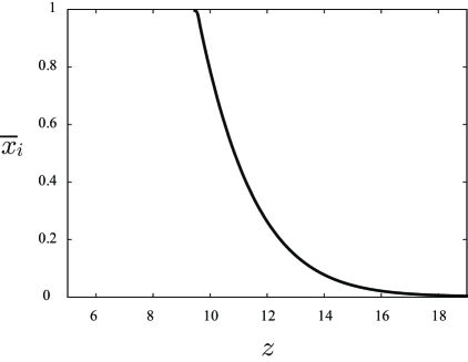
Figure 1: The redshift evolution of the ionized fraction. we adopt $\zeta=40$ and $m_{\rm min}$ corresponding to the virial temperature $T_{\rm vir}=10^{4}~{}$K.

4 Effects of the primordial non-Gaussianity

Primordial non-Gaussianities modify the abundance, merger history and clustering of dark halos (Dalal et al., 2008; Slosar et al., 2008). These effects will evidently induce the early beginning of the reionization process, even though the effect on the reionization optical depth is not very strong. For example, the local type non-Gaussianity with $f_{\rm NL}=100$ will only enhance the optical depth by $1\%$ (Crociani et al., 2009). Therefore we assume that the redshift evolution of the background ionized fraction obtained in the previous section is not modified by the existence of the non-Gaussianity. However, as reionization sources are collapsed objects in the fluctuation of the density field, the fluctuations of the ionized fraction can be affected strongly by primordial non-Gaussianity.

Dalal et al. (2008) have studied the effect of $f_{\rm NL}$ on peak heights of the density fluctuations and the bias of density tracers. According to Eq. (9) in Dalal et al. (2008), we can write the bias of density fluctuations of ionized fraction with primordial non-Gaussianity is given by

$$b_{\rm NG}=b_{x}+2(b_{x}-1)f_{\rm NL}\delta_{B}{3\Omega_{m}H_{0}^{2}\over 2aD(a)k^{2}T(k)},$$ (17)

where T(k) is the transfer function ($T(k)\sim 1$ on large scales), $\delta_{B}$ is the critical density for the bias tracer. In this paper, the bias tracer is the ionized cell. Therefore we adopt the critical density for the ionized cell, while the critical density is for collapse, $\delta_{c}$, in Dalal et al. (2008).

Since the ionized fraction is almost unity in an ionized cell, $\zeta f_{\rm coll}\gg 1$ in such a cell. Therefore we assume that the condition for the ionized cell is $\zeta f_{\rm coll}>1$. This condition gives the critical density for the ionized cell,

$$\delta_{B}\equiv\delta_{c}-\sqrt{2}K(\zeta)[\sigma_{\rm min}^{2}-\sigma_{2}(m)]^{1/2},$$ (18)

where $K(\zeta)={\rm erf}^{-1}(1-\zeta^{-1})$. Eq. (18) corresponds to Eq. (4) in Furlanetto et al. (2004) and Eq. (5) in Joudaki et al. (2011). The primordial non-Gaussianity $f_{\rm NL}$ affect $f_{\rm coll}(\delta)$. However this effect is enough small that we can neglect the modification of $f_{\rm NL}$ on $f_{\rm coll}(\delta)$ ( Joudaki et al. 2011 reported that the mean critical density $\overline{\delta}_{B}$ is only perturbed by 4% even for $f_{\rm NL}=100$). Now we can write the cross-power spectrum between $\delta$ and $\delta_{x}$ with $f_{\rm NL}$ is given by

$$P_{\delta x}(k)=b_{\rm NG}P_{\delta}(k).$$ (19)

Using Eqs. (9) and (19), we calculate the cross-power spectra between CMB and the 21 cm line from $z=11$ for different $f_{\rm NL}$s. We plot the angular power spectrum of the cross-correlation in the top panel of Figure 2. We also show the ratio of the angular spectra between non-Gaussian and Gaussian cases, $R_{\rm NG}=C^{\rm NG}_{\ell}/C^{\rm Gaussian}_{\ell}$, in the bottom panel. Due to the scale dependent bias introduced by $f_{\rm NL}$, the higher $f_{\rm NL}$ induces higher cross-correlation on large scales, while the effect of $f_{\rm NL}$ on the cross-correlation is small on smaller scales ($\ell>100$) and it does not modify the position and the height of the cross-correlation peak. As pointed by Alvarez et al. (2006); Adshead & Furlanetto (2008), the peak height of the cross-correlation depends on the evolution of the ionized fraction. Therefore, these facts suggest that the spectrum of the cross-correlation on large scale have the potential to give the constraint on $f_{\rm NL}$, while one can derive information on the evolution of the cosmic reionization from the peak height and position.

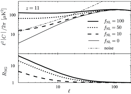
Figure 2: The cross-power spectrum for different $f_{\rm NL}$ (top panel) and the ratio of the cross-power spectrum between non-Gaussian and Gaussian cases (bottom panel). On both panels, the solid, dotted and dashed lines are for $f_{\rm NL}=100$, $f_{\rm NL}=50$ and $f_{\rm NL}=10$, respectively. For comparison, we plot the angular power spectrum for the Gaussian case as the thin solid line on the top panel. The dashed-dotted line represents the noise power spectrum in the combination of Planck and Omniscope.

For the purpose of cross-checks and comparisons, we also calculate the angular power spectrum of 21 cm fluctuations $C_{\ell}^{21}$. According to Eq. (4), $C_{\ell}^{21}$ can be written as

$$C_{\ell}^{21}(z)=T_{21}(z)^{2}\frac{2}{\pi}\int_{0}^{\infty}dk~{}k^{2}\left[(1-\overline{x}_{i}(z))^{2}P_{\delta}(k)J_{\ell}^{2}(kr)-2\overline{x}_{i}(z)(1-\overline{x}_{i}(z))P_{x\delta}J_{\ell}(kr)j_{\ell}(kr)+\overline{x}_{i}(z)P_{xx}j_{\ell}^{2}(kr)\right],$$ (20)

where $P_{xx}$ is the power spectrum of the ionized fraction and is assumed to be $P_{xx}(k)=b_{\rm NG}^{2}P(k)$. Note that we have neglected the redshift distortion here due to the peculiar velocity of baryons. The top panels of Figure 3 shows $C_{\ell}^{21}$ at $z=11$ for different $f_{\rm NL}$ and the bottom panel represents the ratio of the angular spectra between non-Gaussian and Gaussian cases, $R_{\rm NG}$. The angular spectrum on large scales is also amplified by non-zero $f_{\rm NL}$, showing similar behavior in the 21 cm power spectrum as discussed in Joudaki et al. (2011). Compared with the cross-correlation, auto-correlation has a larger amplitude, but the degree of the amplification due to $f_{\rm NL}$ is small on scales $\ell<10$. This is because the term $P_{xx}$ proportional to $b_{\rm NG}^{2}$ is partially canceled by $P_{x\delta}$ on these scales.

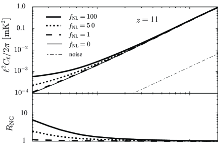
Figure 3: The angular spectrum of 21 cm fluctuations for different $f_{\rm NL}$ (top panel) and the ratio of the angular spectrum spectrum between non-Gaussian and Gaussian cases (bottom panel). We adopt the fiducial reionization model ($\zeta=40$, $T_{\rm vir}=10^{4}~{}$ K). Types of lines are same as in Figure 2. The dashed-dotted line represents the noise power spectrum of Omniscope.

On the other hand, as we can see from Eq. (9), the cross-correlation amplitude includes $\partial\dot{\tau}/\partial\eta$, the amplitude of the cross-correlation depends on the efficiency of the reionization process. We evaluate the cross-correlation in the following rapid reionization model with $\zeta=400$ and $T_{\rm vir}=10^{5}~{}$K. These parameters are motivated by the scenario in which the sources of ionization photons are massive objects like QSOs. We plot the angular power spectrum of the cross-correlation for the rapid reionization model in the top panel and the ratio of the angular spectra between non-Gaussian and Gaussian cases in of Figure 4.

As discussed in Alvarez et al. (2006); Adshead & Furlanetto (2008), the height of the peak is amplified by the rapidness of the reionization process. The amplification due to $f_{\rm NL}$ depends on $\delta_{B}$. According to Eq. (18), $\delta_{B}$ is related to the reionization parameters, $\zeta$ and $T_{\rm vir}$. Large values of $\zeta$ increase $\delta_{B}$, while large values of $T_{\rm vir}$ make $\delta_{B}$ small through decreasing $\sigma_{\rm min}$. As a result, $\delta_{B}$ in the rapid reionization model is almost same as in the fiducial model. Therefore, the dependence of $R_{\rm NG}$ on $f_{\rm NL}$ in the bottom panel of figure 4 is same as in the fiducial model shown in figure 2.

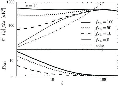
Figure 4: The cross-power spectrum in the rapid reionization model for different $f_{\rm NL}$ (top panel) and the ratio of the angular spectrum spectrum between non-Gaussian and Gaussian cases (bottom panel). Types of lines are same as in Figure 2.The dashed-dotted line represents the noise power spectrum in the combination of Planck and Omniscope.

4.1 The Detectability of the Cross-Correlation

In this section, we calculate the signal-to-noise (S/N) ratio of the cross-correlations in order to study the detectability of the cross-spectrum signal with $f_{\rm NL}$.

If we assume that foreground correlation between CMB and 21 cm can be removed (McQuinn et al., 2006; Morales et al., 2006), the S/N ratio for the cross-correlation can then be expressed as

$$\left({S\over N}\right)^{2}=f_{\rm sky}\sum_{\ell=\ell_{\rm min}}^{\ell_{\rm max}}(2\ell+1){|C_{\ell}^{21-\alpha}|^{2}\over|C_{\ell}^{21-\alpha}|^{2}+(C_{\ell}^{21}+N_{\ell}^{21})(C_{\ell}^{\bm{C}MB}+N_{\ell}^{\bm{C}MB})}.$$ (21)

where $f_{\rm sky}$ is the sky fraction common to both CMB and 21 cm observations, the superscript $21$ stands for 21-cm fluctuations, the superscript $CMB$ stands for the CMB anisotropy, and $C_{\ell}$ and $N_{\ell}$ are the signal and the noise power spectrum, respectively. According to Eq. (21), even if there is no instrumental noise ($N_{\ell}=0$), the S/N ratio is limited by the cosmic variance, especially for small values of $\ell_{\rm max}$. In this paper, since we are interested in large scales, we consider Planck as CMB observation whose sky fraction is almost unity. Therefore $f_{\rm sky}$ corresponds to the one of the considered 21 cm observation. In the Planck configuration, compared with the CMB signal, the experimental noise is very small on our scales of interest, $C_{\ell}^{\rm CMB}\gg N_{\ell}^{\rm CMB}$. Therefore, we neglect $N_{\ell}^{\rm CMB}$ in the calculation.

The noise power spectrum of 21-cm observations is given by

$${N_{\ell}^{21}}={2\pi\over t_{\rm obs}\Delta\nu}\left({\ell_{\rm max}\over 2\pi}{\lambda^{2}T_{\rm sys}\over A_{\rm eff}}\right)^{2}.$$ (22)

where $\Delta\nu$ is the bandwidth, $t_{\rm obs}$ is the total observation time, and $\ell_{\rm max}=2\pi{D/\lambda}$ is the maximum multipole associated with the length of the baseline $D$. The system temperature $T_{\rm sys}$ is dominated by sky temperature which is expressed as $T_{\rm sys}=2.7(1+z)^{2.3}~{}\rm K$ (Bowman et al., 2006). $A_{\rm total}$ is the total effective area which is assumed to be $A_{\rm total}=NA_{\rm eff}$ with N being the number of the antenna and $A_{\rm eff}$ being the effective area of one antenna. For 21 cm observation, we consider an optimistic experiment Omniscope (or FFTT) (Tegmark & Zaldarriaga, 2009). We evaluate the observational noise with $N=10^{6}$, $A_{\rm eff}=1~{}{\rm m}^{2}$, $D=1~{}$km, $t_{\rm obs}=4000~{}$hours and $f_{\rm sky}=2\pi$ (Mao et al., 2008). We plot the estimated noise power spectrum as the dashed-dotted lines in Fig. 2 and 4.

We also show the noise power spectrum of Omniscope in the auto-correlation of 21 cm fluctuations in Fig. 3. Compared with the auto-correlation, the noise of the cross-correlation is large in particular, on small scales, because CMB Doppler signal from the EoR is proportional to $k^{-1}$ and the primordial CMB signal gives large noise on small scales.

We then calculate the S/N ratio for the cross-correlation for the fiducial reionization case ($\zeta=40$ and $T_{\rm vir}=10^{4}$). The left panel of Fig. 5 shows the dependence of the S/N ratio on the values of $f_{\rm NL}$. As discussed above, the amplification due to $f_{\rm NL}$ arises on large scales. However, the cosmic variance is significant on such scales Accordingly, the S/N ratio is suppressed on small $\ell_{\rm max}$. As $\ell_{\rm max}$ increases, the S/N ratio also goes up until $\ell\sim 100$ where the noise power spectrum of the 21 cm observation dominate the cross-correlation signal completely. The existence of $f_{\rm NL}$ brings relatively high S/N ratio, compared with the case for $f_{\rm NL}=0$. However, since the amplification due to $f_{\rm NL}$ becomes small on small scales, the S/N ratio has weak dependence on $f_{\rm NL}$.

Fig. 5 shows that, while the amplitude of the cross-correlation enhances with $f_{\rm NL}$ increasing, the S/N ratio decreases with $f_{\rm NL}$ increasing. For example, the S/N ratio is $2.4$ for $f_{\rm NL}=100$ and is $2.8$ for $f_{\rm NL}=10$ with $l_{\rm max}=200$. This is because large $f_{\rm NL}$ also increases $C_{\ell}^{21}$ appearing in the denominator in Eq. (21). However the amplification due to $f_{\rm NL}$, $R_{\rm NG}$, for the auto-correlation in Fig. 3 is suppressed for small $f_{\rm NL}$, compared with $R_{\rm NG}$ for the cross-correlation in Fig. 2. As a result, small values of $f_{\rm NL}$ gives the large S/N ratio. In the case for $f_{\rm NL}<10$, the amplification of the cross-correlation due to $f_{\rm NL}$ becomes small. Therefore the S/N ratio also starts to decrease with $f_{\rm NL}$ getting lower for $f_{\rm NL}<10$.

On the other hand, the auto power spectrum completely dominate the noise power spectrum of Omniscope as in Fig. 3. Therefore the S/N ratio is large and $S/N\sim\ell_{\rm max}$ even for $\ell_{\rm max}\sim 10$. the Omniscope auto power-spectrum S/N ratio is large and For comparison, we evaluate the $S/N$ ratio in SKA, where we adopt $N=1400$, $A_{\rm eff}=45~{}{\rm m}^{2}$, $D=0.01~{}$Km and $f_{sky}=0.0056$ (Joudaki et al., 2011). The S/N ratio is 3.8 for $\ell_{max}=50$ for each $f_{\rm NL}$, although the S/N ratio is 1.6 for $\ell_{max}=20$. This suggests that in the absence of significant foregrounds and systematics, the auto-correlations of 21 cm is a better probe than the cross-correlations (as expected since it depends on $b^{2}$), while the cross-correlations has only 1 factor of $b$. Nevertheless, it is interesting to look at the cross-correlations, since it is more likely we can rid of systematics and foregrounds that are common to both CMB and 21 cm experiments.

The rapid reionization case with $\zeta=400$ and $T_{\rm vir}=10^{5}~{}$K brings high S/N ratio. Our estimated S/N ratio for the rapid reionization case is $2.7$ for $f_{\rm NL}=10$ and $3.2$ for $f_{\rm NL}=10$ as shown in the right panel of Fig. 5. Therefore, this fact suggests that any detection of excess power in the cross-correlation with relatively high S/N ratio implies the efficient reionization process and the existence of high $f_{\rm,NL}$.

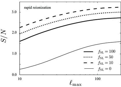
Figure 5: The dependence of the S/N ratio on $\ell_{\rm max}$ for the combination of Planck and Omniscope. The left and right panels show for the fiducial (slow) and rapid reionization model, respectively. Types of lines are same as in Figure 2.

5 Conclusion and Discussion

In this paper we have studied the potential of the cross-correlation between CMB temperature anisotropies and 21 cm fluctuations from EoR to constrain the primordial non-Gaussianities. Assuming the analytic reionization model, we have utilized the effect of primordial non-Gaussianity on the bias of the ionized fraction fluctuations. We have calculated the cross-correlation to the linear order and shown the angular cross-power spectrum, while contrasting against 21 cm auto power-spectrum.

Due to the scale dependent nature of the effect of primordial non-Gaussianity, the effect is larger at large scales. The higher $f_{\rm NL}$ become, the more the angular power spectrum is enhanced, and the enhancement is more significant in lower multipoles. Since the amplitude of the cross-correlation depends on the efficiency of the reionization, we also investigated the effect of different reionization models on the cross power-spectrum. The overall amplitude of cross-power in the rapid reionization model is higher than the overall amplitude of cross-power in the slow reionization model. The amplification due to the non-Gaussianity, $R_{\rm NG}$, depends on the critical density, $\delta_{B}$, of the ionized bubbles. However, in our reionization model, we found that the dependence of $\delta_{B}$ on the ionization parameter is weak. As a result, $R_{\rm NG}$ are almost same in both the fiducial and rapid reionization models. This suggests that the determination of $f_{\rm NL}$ from $R_{\rm NG}$ does not degenerate with other reionization parameters strongly.

The degree of the amplification due to $f_{\rm NL}$ in the cross-correlation is larger on $\ell\gtrsim 10$ than the corresponding scale in auto-correlation of the 21 cm fluctuations. However, the CMB Doppler signal becomes small on small scales and is dominated by the primordial CMB signal. This makes the noise large and the detection of the cross-correlation difficult, when compared against the auto-correlation of the 21 cm fluctuations.

To access the detectability, we have calculated the signal-to-noise (S/N) ratio of both auto- and cross-power of Omniscope. In the case of the fiducial (slow) reionization model, the S/N ratio is 2.4 for $f_{\rm NL}=100$ and become 2.8 for $f_{\rm NL}=10$. Since high $f_{\rm NL}$ enhances the auto-power spectrum which increases the noise for the cross-correlation signal, high $f_{\rm NL}$ brings small S/N ratio and we obtain the maximum S/N ratio at $f_{\rm NL}=10$. In the rapid reionization, the S/N ratio is enhanced for all $f_{\rm NL}>0$. Since the amplification due to $f_{\rm NL}$, $R_{\rm NG}$, does not depends on the reionization parameters, the enhancement of the S/N ratio in the rapid suggest that $f_{\rm NL}$ is well determined in the rapid reionization model.

In comparison, the S/N ratio for the auto-correlation is quite large. Even for SKA, the S/N ratio becomes 3.8 for $l_{\rm max}=50$. This suggests that in the absence of significant foregrounds and systematics, the auto-correlations of 21 cm is a better probe than the cross-correlations (as expected since it depends on $b^{2}$), while the cross-correlations contains only 1 factor of $b$. Nevertheless, it is interesting to look at the cross-correlations, since it is more likely we can rid of systematics and foregrounds that are common to both CMB and 21 cm experiments than completely clean 21 cm of all of the possible foregrounds and systematics in large scales. In the calculation of the S/N ratio, we ignore the foreground contamination of the cross-correlation between CMB and 21cm fluctuations. In reality, some of the foregrounds for 21-cm observations also have the correlation with CMB observations (Adshead & Furlanetto, 2008). This may affect significantly the detection of the signal. Therefore a better model of the foreground is essential for any 21 cm constraint on the non-Gaussianity. The tidal approach suggested by Pen et al. (2012) can be a potential technique to reduce such foreground contamination from 21 cm mapping.

In the paper, we consider only one redshift slice for the 21 cm observation in this paper. We can observe many redshift slices by choosing the observation frequency. According to Eq. (21), taking many redshift slices would increase S/N ratio for each $f_{\rm NL}$. As a result, multi-frequency observation of 21 cm fluctuations can bring the better constraint on $f_{\rm NL}$ than the one redshift slice such as considered in this paper. In particular, the S/N ratio for the auto-correlation receives benefit richly from multi-frequency observation. It can be expected that even the S/N ratio for SKA become enough to measure the non-Gaussianity as studied in Joudaki et al. (2011). On the other hand, the signal of the cross-correlation in the redshift evolution reaches a peak during the epoch when the ionized fraction becomes a half (Alvarez et al., 2006). In particular, in contrast to the case of the rapid reionization, there is possibility to utilize many redshift slices for 21 cm fluctuations in the case of the slow reionization, as the cross-correlation signals arises during a long period due to the slow evolution of the ionized fractions.

Finally, we focus the signals from the EoR on large scales. However it is well-known that the distribution of the bubbles affect CMB anisotropies and 21 cm fluctuations (Iliev et al., 2006; Furlanetto et al., 2004). Therefore, the effect of non-Gaussianity can be expected to arise on small scales. We will leave this to future work.

References

- Adshead & Furlanetto (2008) Adshead, P. J., Furlanetto, S. R. 2008, MNRAS, 384, 291
- Alvarez et al. (2006) Alvarez M. A., Komatsu E., Doré O., Shapiro P. R., 2006, Astrophys. J., 647, 840
- Bardeen et al. (1983) Bardeen J. M., Steinhardt P. J., Turner M. S., 1983, Phys.Rev.D, 28, 679
- Barkana & Loeb (2001) Barkana, R., Loeb, A. 2001, Phys.Rep., 349, 125
- Bartolo et al. (2004) Bartolo N., Komatsu E., Matarrese S., Riotto A., 2004, Phys.Rep, 402, 103
- Bharadwaj & Ali (2004) Bharadwaj S., Ali S. S., 2004, MNRAS, 352, 142
- Bowman et al. (2006) Bowman J. D., Morales M. F., Hewitt J. N., 2006, Astrophys. J., 638, 20
- Carilli &Rawlings (2004) Carilli, C. L., Rawlings, S. 2004, New Astron.Rev., 48, 979
- Ciardi & Madau (2003) Ciardi B., Madau P., 2003, Astrophys. J., 596, 1
- Crociani et al. (2009) Crociani, D., Moscardini, L., Viel, M., Matarrese, S. 2009, MNRAS, 394, 133
- Curto et al. (2009) Curto A., Martínez-González E., Barreiro R. B., 2009, Astrophys. J., 706, 399
- Dalal et al. (2008) Dalal N., Doré O., Huterer D., Shirokov A., 2008, Phys.Rev.D, 77, 123514
- Desjacques & Seljak (2010) Desjacques V., Seljak U., 2010, Classical and Quantum Gravity, 27, 124011
- Falk et al. (1993) Falk T., Rangarajan R., Srednicki M., 1993, Astrophys. J. L., 403, L1
- Furlanetto (2006) Furlanetto S. R., 2006, MNRAS, 371, 861
- Furlanetto et al. (2004) Furlanetto S. R., Zaldarriaga M., Hernquist L., 2004, Astrophys. J., 613, 1
- Furlanetto et al. (2004) Furlanetto, S. R., Zaldarriaga, M., Hernquist, L., 2004, Astrophys. J., 613, 16
- Gangui et al. (1994) Gangui A., Lucchin F., Matarrese S., Mollerach S., 1994, Astrophys. J., 430, 447
- Guth & Pi (1982) Guth A. H., Pi S., 1982, Phys. Rev. Lett., 49, 1110
- Harker et al. (2010) Harker, G., Zaroubi, S., Bernardi, G., et al. 2010, MNRAS, 405, 2492
- Iliev et al. (2006) Iliev, I. T., Pen, U.-L., Richard Bond, J., Mellema, G., Shapiro, P. R. 2006, New Astronomy Reviews, 50, 909
- Joudaki et al. (2011) Joudaki S., Dore O., Ferramacho L., Kaplinghat M., Santos M. G., 2011, Phys. Rev. Lett. 107 131304
- Kaiser (1987) Kaiser N., 1987, MNRAS, 227, 1
- Komatsu & Spergel (2001) Komatsu E., Spergel D. N., 2001, Phys.Rev.D, 63, 063002
- Komatsu (2011) Komatsu E. et. al., 2011, ApJS, 192, 18
- Lonsdale et al. (2009) Lonsdale, C. J., Cappallo, R. J., Morales, M. F., et al. 2009, IEEE Proceedings, 97, 1497
- Madau et al. (1997) Madau P., Meiksin A., Rees M. J., 1997, Astrophys. J., 475, 429
- Mao et al. (2008) Mao Y., Tegmark M., McQuinn M., Zaldarriaga M., Zahn O., 2008, Phys.Rev.D, 78, 023529
- McQuinn et al. (2006) McQuinn, M., Zahn, O., Zaldarriaga, M., Hernquist, L., & Furlanetto, S. R. 2006, Astrophys. J., 653, 815
- Morales et al. (2006) Morales, M. F., Bowman, J. D., & Hewitt, J. N. 2006, Astrophys. J., 648, 767
- Slosar et al. (2008) Slosar A., Hirata C., Seljak U., Ho S., Padmanabhan N., 2008, JCAP, 8, 31
- Smidt et al. (2009) Smidt J., Amblard A., Serra P., Cooray A., 2009, Phys.Rev.D, 80, 123005
- Starobinsky (1982) Starobinsky A. A., 1982, Physics Letters B, 117, 175
- Tashiro et al. (2010) Tashiro H., Aghanim N., Langer M., Douspis M., Zaroubi S., Jelić V., 2010, MNRAS, 402, 2617
- Tashiro & Sugiyama (2012) Tashiro H., Sugiyama N., 2012, MNRAS, 420, 441
- Tegmark & Zaldarriaga (2009) Tegmark M., Zaldarriaga M., 2009, Phys.Rev.D, 79, 083530
- Tegmark & Zaldarriaga (2010) Tegmark M., Zaldarriaga M., 2010, Phys.Rev.D, 82, 103501
- The Planck Collaboration (2006) Planck Collaboration Blue-book, ”Planck, The Scientific Program”, ESA-SCI (2005)
- Pen et al. (2012) Pen, U.-L., Sheth, R., Harnois-Deraps, J., Chen, X., & Li, Z. 2012, arXiv:1202.5804