Solving the mode identification problem in asteroseismology of F stars observed with Kepler

Abstract

Asteroseismology of F-type stars has been hindered by an ambiguity in identification of their oscillation modes. The regular mode pattern that makes this task trivial in cooler stars is masked by increased linewidths. The absolute mode frequencies, encapsulated in the asteroseismic variable $\epsilon$, can help solve this impasse because the values of $\epsilon$ implied by the two possible mode identifications are distinct. We find that the correct $\epsilon$ can be deduced from the effective temperature and the linewidths and we apply these methods to a sample of solar-like oscillators observed with Kepler.

1. Introduction

Asteroseismology of solar-like stars is developing rapidly, driven by the successes of the space telescopes CoRoT (Michel et al., 2008) and Kepler (Koch et al., 2010; Gilliland et al., 2010; Chaplin et al., 2011). By studying the oscillation modes of these stars, inferences can be made about their interior structures (e.g. Verner et al., 2011). Except for the most basic analyses, it is crucial to identify the oscillation modes, that is, the radial order $n$ and the spherical degree $l$.

In the Sun and similar stars, mode identification is straightforward thanks to the distinctive pattern of alternating odd and even modes in the power spectrum. This pattern consists of a regular sequence of $l=1$ modes, interspersed with close pairs of $l=0$ and 2 modes that fall approximately halfway in between. However, stars significantly hotter than the Sun have large linewidths that blur the $l=0,2$ pairs and make mode identification very difficult. In this Letter we demonstrate a solution to this problem that applies the method proposed by Bedding & Kjeldsen (2010) and White et al. (2011a), which uses the absolute frequencies of the oscillation modes.

2. Methods

For main-sequence stars, the frequencies are well-approximated by the asymptotic relation (Vandakurov, 1967; Tassoul, 1980; Gough, 1986),

$$\nu_{n,l}\approx\Delta\nu\left(n+{l\over 2}+\epsilon\right)-\delta\nu_{0l}.$$ (1)

Here, $\Delta\nu$ is the large separation between modes of the same degree $l$ and consecutive order $n$, $\delta\nu_{0l}$ is the small separation between modes of different degree and $\epsilon$ is a dimensionless offset, which we discuss in greater detail below. Typically, only modes of $l\leq 2$ are observed in intensity due to cancellation over the unresolved stellar disk, although $l=3$ modes can be observed in the highest signal-to-noise targets, such as 11 Kepler subgiants for which frequencies have been determined by Appourchaux et al. (2012b) and the solar analogs 16 Cyg A and B Metcalfe et al. (2012).

Figure 1.— Power spectra of (a) a G star, KIC 6933899, and (b) an F star, KIC 2837475, with their corresponding échelle diagrams (c) and (d), respectively. The red curves show the power spectra after smoothing. Mode identification of the G star is trivial, with modes of $l=0$ (orange), 1 (blue) and 2 (green) labeled. For the F star it is not clear whether the peaks labeled ‘A’ (blue) or ‘B’ (orange) correspond to the $l=1$ or $l=0,2$ modes.

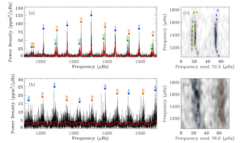
The asymptotic relation makes it easy to determine the mode degrees for the Sun and similar stars. Each $l=0$ mode is separated by $\delta\nu_{02}$ from an $l=2$, and separated by $\Delta\nu/2-\delta\nu_{01}$ from the $l=1$ mode of the same order. An example is shown in Figure 1a for the Kepler star KIC 6933899, which has an effective temperature of 5840 K.

Mode linewidth increases with effective temperature (Chaplin et al., 2009; Baudin et al., 2011; Appourchaux et al., 2012a; Corsaro et al., 2012), reflecting shorter mode lifetimes in hotter stars. In some F-type stars, the linewidths become so large that the pairs of $l=0$ and $l=2$ modes are unresolved and it becomes difficult to distinguish between the blended $l=0,2$ modes and the $l=1$ modes. This problem was first observed by CoRoT, in the F5 star HD 49933 (Appourchaux et al., 2008) and has since been seen in other CoRoT stars (Barban et al., 2009; García et al., 2009) and in the bright F5 star Procyon (Bedding et al., 2010b). We also see it in many Kepler stars and Figure 1b shows one example, KIC 2837475 ($T_{\mathrm{eff}}=6690$ K).

One way to resolve this identification problem is to fit both possible mode identifications and compare the relative likelihoods of the two scenarios (Appourchaux et al., 2008; Benomar et al., 2009; Gruberbauer et al., 2009; Kallinger et al., 2010; Bedding et al., 2010b; Handberg & Campante, 2011). This relies on the profile of the even-$l$ modes being significantly broader and also asymmetric, relative to the $l=1$ modes (owing to the presence of the smaller amplitude $l=2$ modes at a slightly lower frequency than the $l=0$ modes). The correct scenario should provide a better fit to the power spectrum. Difficulties arise at low signal-to-noise and with short observations, for which the Lorentzian mode profiles are not well resolved. This method was first applied by Appourchaux et al. (2008), who fitted both scenarios for HD 49933. However, with additional data their preferred mode identification was overturned by Benomar et al. (2009).

Other methods have been suggested that utilize the sign of the small separation $\delta\nu_{01}$ (Roxburgh, 2009; Mosser & Appourchaux, 2009). In main sequence stars like the Sun, $\delta\nu_{01}$ is known to be positive. However, in many red giants $\delta\nu_{01}$ is found to be negative (Bedding et al., 2010a; Huber et al., 2010; Mosser et al., 2011), so at some point in the evolution the sign must flip (Stello, 2011). To further complicate matters, the value of $\delta\nu_{01}$ is quite small. At low signal-to-noise, it may be difficult to obtain frequencies precise enough to determine the sign of $\delta\nu_{01}$ reliably.

Bedding & Kjeldsen (2010) have suggested that scaling the frequencies of a star with a known mode identification could reveal the correct mode identification in a second star. This method seeks to use information contained within the value of $\epsilon$. For this to be effective, $\epsilon$ must vary slowly as a function of stellar parameters. This is indeed the case, with a tight relationship between $\epsilon$ and effective temperature, $T_{\mathrm{eff}}$, found both in models (White et al., 2011b) and in observations of Sun-like stars (White et al., 2011a). Thus, $\epsilon$ promises to be an effective way to determine mode identifications, since the difference in the value of $\epsilon$ for the two possible scenarios is large (0.5).

The existence of a relation between $\epsilon$ and $T_{\mathrm{eff}}$ is not surprising. The value of $\epsilon$ is determined by the upper and lower turning points of the acoustic waves (e.g. Gough, 1986). As such, $\epsilon$ is heavily dependent upon the stellar atmosphere, of which $T_{\mathrm{eff}}$ is a significant parameter. Due to inadequate modeling of the near-surface layers, there is a well-known offset between observed and computed oscillation frequencies in the Sun (Christensen-Dalsgaard et al., 1988; Dziembowski et al., 1988; Christensen-Dalsgaard et al., 1996; Christensen-Dalsgaard & Thompson, 1997) and also in other stars (Kjeldsen et al., 2008; White et al., 2011a; Mathur et al., 2012). This offset results in the computed $\epsilon$ being smaller than observed, typically by $\sim 0.2$ as inferred from the displacement of model tracks from observations in the $\epsilon$ diagram.

The purpose of this Letter is to extend the relationship between $\epsilon$ and $T_{\mathrm{eff}}$ to higher temperatures, and thereby make reliable mode identifications in F-type stars.

3. Observations and Data Analysis

We used observations of solar-like oscillations in 163 stars taken with the Kepler space telescope between May 2009 and March 2011 (Quarters 1–8). Each star was observed in Kepler’s short-cadence mode (58.9 s sampling) for part of this period. The time series were prepared from the raw observations as described by Jenkins et al. (2010) and further corrected to remove outliers and jumps as described by García et al. (2011).

Figure 2.— Modified H-R diagram: average large frequency separation, $\Delta\nu$, against effective temperature for stars in our sample. Stars with secure mode identifications are indicated by black circles. Those without are red squares. Grey lines are ASTEC (Christensen-Dalsgaard, 2008) evolutionary tracks for a metallicity of $Z_{0}=0.011$ ($[\mathrm{Fe/H}]=-0.2\,\mathrm{dex}$), matching the $T_{\mathrm{eff}}$ calibration of Pinsonneault et al. (2011). The dashed line indicates approximately the cool edge of the classical instability strip (Saio & Gautschy, 1998).

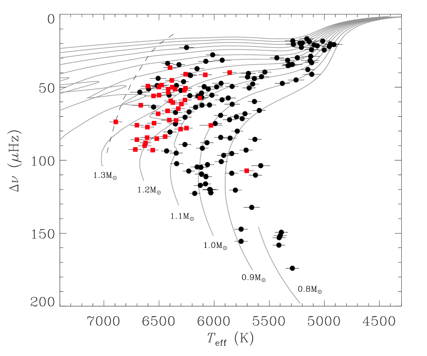
Effective temperatures were determined from SDSS $griz$ color-temperature relations by Pinsonneault et al. (2011). Spectroscopic temperatures have also been determined for 77 stars in our sample by Bruntt et al. (2012). In almost all cases the photometric and spectroscopic temperatures agree, except for several stars where the disagreement may be due to differing metallicities or unresolved binaries (the temperatures for KIC 3424541, 3456181, 4638884, 6679371, 7976303, 8938364, 9908400, 10018963, 10124866 and 10963065 were found to disagree by more than 3$\sigma$). Figure 2 shows a modified HR diagram of this sample, where we have used large separation instead of luminosity.

To measure the value of $\epsilon$ for each star, we first determined the frequencies of the $l=0$ modes. Where it was possible to resolve the $l=0$ and $l=2$ modes, we measured the frequencies of the $l=0$ modes from the peak in the power spectrum after smoothing. This was possible for 115 stars. An example is shown in Figure 1a.

Where it was not possible to resolve the $l=0$ and $l=2$ modes, and therefore not possible to easily determine the correct mode identification, we determined $\epsilon$ for both scenarios (43 stars). In this case we used the frequencies of the ridge centroids, determined from the peaks of the heavily smoothed power spectrum, as shown in an example F star in Figure 1b. There were also two cooler stars for which the mode identification was not clear (KIC 11401708 and 12555505); these have low signal-to-noise and the $l=2$ modes are not apparent.

For five stars with blended $l=0$ and $l=2$ modes it was still possible to make an unambiguous mode identification (KIC 6064910, 6766513, 7668623, 7800289 and 8026226). In these stars, avoided crossings ‘bump’ the $l=1$ modes from their asymptotically expected position (Osaki, 1975; Aizenman et al., 1977), revealing the correct identification. In these five cases, the frequencies were obtained from the centroids of the $l=0,2$ ridge.

The values of $\Delta\nu$ and $\epsilon$ were obtained from a weighted least-squares fit to the $l=0$ frequencies, as described by White et al. (2011b). The weights were given by a Gaussian function centered at the frequency of maximum power, $\nu_{\mathrm{max}}$, with a FWHM of $0.25\,\nu_{\mathrm{max}}$. By the asymptotic relation, equation 1, the gradient of this fit is $\Delta\nu$ and the y-intercept is $\epsilon\Delta\nu$.

To confirm the validity of our method of frequency determination, we compared the values of $\epsilon$ derived from our frequencies to those derived from frequencies that have been determined by more traditional ‘peak-bagging’ methods in the 61 stars for which this has been done (Appourchaux et al., 2012b). We found good agreement, with $\epsilon$ values typically agreeing to within 0.1, which is approximately the size of the typical uncertainty. This agreement is of particular importance for hotter stars because using ridge centroids instead of $l=0$ frequencies potentially biases $\epsilon$ towards slightly lower values. We found this bias to be negligible within the uncertainties.

4. Results

Figure 3.— The $\epsilon$ diagram: large separation, $\Delta\nu$, against $\epsilon$. (a) Only stars with secure mode identifications are shown (filled black circles). Lines are ASTEC evolutionary tracks, as shown in Figure 2, although for clarity, segments of the tracks which are hotter than the approximate cool edge of the instability strip are not shown. Note the offset between models and observations. (b) Symbol colors reflect the measured effective temperature of the star. Stars with obvious identifications are circles, and those for which we can reliably make the identification from the $\epsilon$–$T_{\mathrm{eff}}$ relation are indicated by diamonds. The possible identifications of one star for which the identification is still ambiguous in the $\epsilon$–$T_{\mathrm{eff}}$ plane is indicated by the encircled squares. Comparing the possible identifications with the temperatures of stars of similar $\Delta\nu$, the scenario on the left can be preferred.

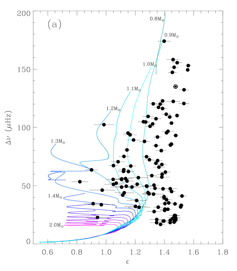
In Figure 3a we show the so-called $\epsilon$ diagram for the 120 Kepler stars whose mode identifications were unambiguous. The observed values of $\epsilon$ are clearly offset to the right of the models which, as mentioned above, arises from the improper modeling of the near-surface layers. From this figure it appears that the offset in $\epsilon$ may be roughly the same for all stars, which corresponds to a fixed fraction of the large separation, as was also inferred by Mathur et al. (2012).

Figure 4.— (a) $\epsilon$ as a function of effective temperature. Stars with unambiguous mode identifications are indicated by blue circles. Stars with ambiguous identifications have two possible values of $\epsilon$ (gray circles) corresponding to the two possible identifications. Several stars for which the width of the relation between $\epsilon$ and $T_{\mathrm{eff}}$ makes the identification difficult are red circles. The scenarios of an example star for which we use $\Delta\nu$ to aid in the identification is circled, as it is in Figure 3b. (b) Same as (a), but showing $\epsilon$ as a function of mode linewidth, $\Gamma$. (c) The selected identification for all stars shown in the $\epsilon$–$T_{\mathrm{eff}}$ plane. The outlier is KIC 1725815, for which $\Gamma$ and $T_{\mathrm{eff}}^{\mathrm{phot}}$ disagree (see text). In all panels the Sun is indicated by its usual symbol. Identifications of Procyon are indicated by magenta diamonds; those of the CoRoT F stars HD 49933 and HD 181420 are orange triangles.

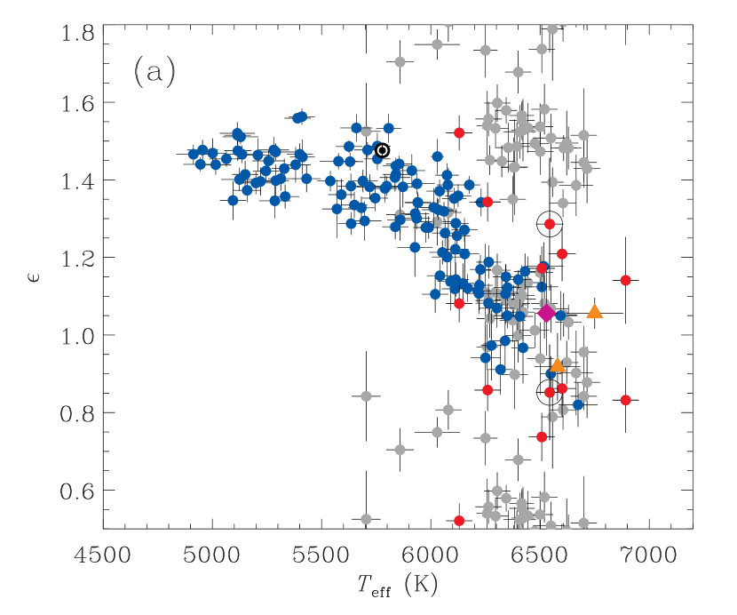
In Figure 4a we show $\epsilon$ versus $T_{\rm eff}$ for our sample. The Sun is marked in black by its usual symbol, and the stars with unambiguous mode identifications are colored blue. The trend of decreasing $\epsilon$ with increasing $T_{\mathrm{eff}}$ is clearly seen in these stars.

For the 43 Kepler stars whose mode identifications are uncertain, the relationship between $\epsilon$ and $T_{\mathrm{eff}}$ can help. In Figure 4a these stars are shown in gray for both scenarios. Owing to the potential ambiguity in $n$, each scenario is also plotted shifted by $\pm 1$. We also include both scenarios of the F stars Procyon (Bedding et al., 2010b), HD 49933 (Appourchaux et al., 2008) and HD 181420 (Barban et al., 2009).

For most of the stars with ambiguous mode identifications, only one of the scenarios lies along the $\epsilon$–$T_{\mathrm{eff}}$ trend defined by the stars with secure identifications and we adopt this as the correct one. For the previously studied F stars, we prefer Scenario B of Procyon (Bedding et al., 2010b), Scenario B of HD 49933 (Benomar et al., 2009) and Scenario 1 of HD 181420 (Barban et al., 2009). Due to the width of the $\epsilon$–$T_{\mathrm{eff}}$ relation, there are a few stars for which the situation is still somewhat ambiguous (red circles in Figure 4a). The two scenarios in these stars have values of $\epsilon$ that fall towards the top and bottom of the relation. For these stars we must use additional information to resolve the ambiguity.

To overcome the spread in the $\epsilon$–$T_{\mathrm{eff}}$ relation, the value of $\Delta\nu$ is useful. For a given effective temperature, stars with higher masses have smaller values of $\Delta\nu$, as can be seen from the models in Figure 2. Models also indicate that higher-mass stars have a smaller $\epsilon$ (see Figure 3a and White et al., 2011b). It follows that in the $\epsilon$–$T_{\mathrm{eff}}$ plane, stars that fall towards the bottom of the trend will be more massive and should therefore have smaller values of $\Delta\nu$ than lower-mass stars of similar temperature.

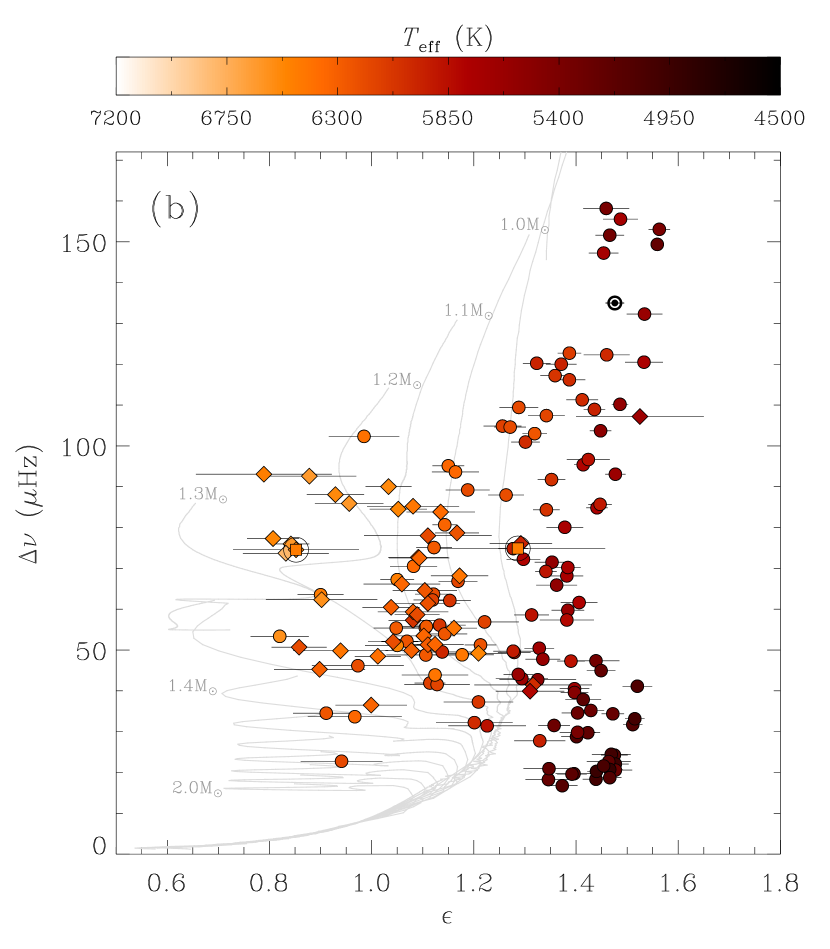
We illustrate this in the $\Delta\nu$–$\epsilon$ plane in Figure 3b, where we show stars in which the identification was already obvious, as well as those for which the identification could be readily made from the $\epsilon$–$T_{\mathrm{eff}}$ relation. Symbols are colored according to $T_{\mathrm{eff}}$, with the trend of decreasing $T_{\mathrm{eff}}$ with increasing $\epsilon$ quite clear. The gradual decrease in $\epsilon$ with decreasing $\Delta\nu$ along lines of constant temperature is also visible. By comparing a star whose identification is still ambiguous with stars of a similar large separation, we can better make a decision on the identification. We show the example of KIC 11290197, whose two scenarios are circled in Figures 3b and 4a. By comparing its $T_{\mathrm{eff}}$ with stars of a similar $\Delta\nu$, we establish the preferred scenario, which in this case has the lower value of $\epsilon$.

Other seismic parameters may also be useful. The method of Mosser et al. (2010), which uses the value of the small separation $\delta\nu_{01}$, agrees for all stars, except one (KIC 5431016), which has a low signal-to-noise.

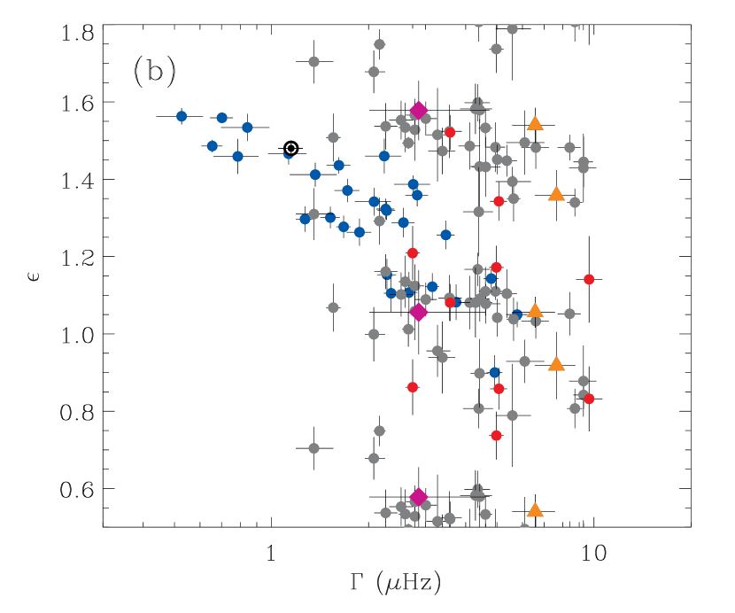
Another very useful parameter is mode linewidth ($\Gamma$). As mentioned above, linewidth is strongly correlated with effective temperature, and so there should also be a correlation between linewidth and $\epsilon$. Linewidths for 41 of our stars (including 12 with ambiguous identifications) were previously measured by Appourchaux et al. (2012a). Using the SYD method described in that paper, we have measured linewidths in a further 26 stars with ambiguous identifications (excluding the five ambiguous stars with the lowest signal-to-noise). Figure 4b shows the relation between $\Gamma$ and $\epsilon$ for these 67 stars.

We can quantify the likelihood of one scenario over the other by comparing how far each lies from the various relations. To do so, we first performed a Bayesian linear fit to the $\epsilon$–$T_{\mathrm{eff}}$ and $\epsilon$–$\ln(\Gamma)$ relations for all stars with $T_{\mathrm{eff}}>5800$ K with unambiguous identifications (i.e. the blue points in Figures 4a and b). For all stars with an uncertain identification, we then calculated the likelihood of obtaining the observed $T_{\mathrm{eff}}$ for each of the two possible values of $\epsilon$ ($\epsilon_{\mathrm{A}}$ and $\epsilon_{\mathrm{B}}$), the observed $\Gamma$, the parameters of the linear fits, and all respective uncertainties. Full details of this method will be provided in a future paper (M. Gruberbauer et al. 2012, in prep.). The required integration over the parameter space was carried out using MultiNest (Feroz et al., 2009). These two likelihood values, $P(T_{\mathrm{eff}}|\epsilon_{\mathrm{A}},\Gamma)$ and $P(T_{\mathrm{eff}}|\epsilon_{\mathrm{B}},\Gamma)$, were then used to calculate the Bayes factor (ratio of the likelihoods), and hence the odds ratio and probability of each scenario, $P(\epsilon_{\mathrm{A}}|T_{\mathrm{eff}},\Gamma)$ and $P(\epsilon_{\mathrm{B}}|T_{\mathrm{eff}},\Gamma)$, assuming equal prior probability for both identifications. We performed this calculation using both photometric and spectroscopic effective temperatures, where available. Our preferred identification is the one with the greatest probability. We denote the value of $\epsilon$ for the preferred identification as $\epsilon_{\mathrm{pref}}$, and use $\epsilon_{\mathrm{alt}}$ for the alternate value.

In Table 1 we list for each star its measured $\Delta\nu$, the value of $\epsilon_{\mathrm{pref}}$ and $\epsilon_{\mathrm{alt}}$, $\Gamma$, both effective temperatures, $T_{\mathrm{eff}}^{\mathrm{phot}}$ and $T_{\mathrm{eff}}^{\mathrm{spec}}$, and the probabilities, $P(\epsilon_{\mathrm{pref}}|T_{\mathrm{eff}}^{\mathrm{phot}},\Gamma)$ and $P(\epsilon_{\mathrm{pref}}|T_{\mathrm{eff}}^{\mathrm{spec}},\Gamma)$, of our preferred scenario. For most of the stars we find strong support for our preferred scenario. One star (KIC 1725815), without a measured $T_{\mathrm{eff}}^{\mathrm{spec}}$, is an outlier in the $\epsilon$–$T_{\mathrm{eff}}$ plane. While the linewidth supports one scenario, $T_{\mathrm{eff}}^{\mathrm{phot}}$ supports the alternate scenario. It is not entirely clear which is correct,although the method of Mosser et al. (2010) agrees with the alternate scenario favored by $T_{\mathrm{eff}}^{\mathrm{phot}}$. Spectroscopic measurement of the temperature may help resolve this case.

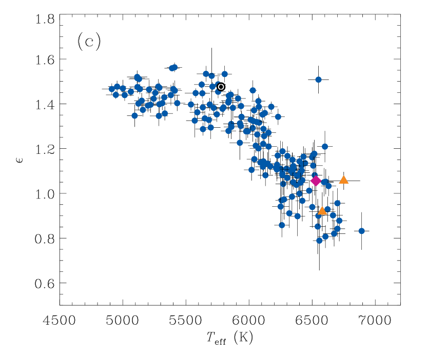
The $\epsilon$–$T_{\mathrm{eff}}$ relation for the final selected identification of all stars in our sample is shown in Figure 4c.

Table 1Measurements of $\Delta\nu$, $\epsilon_{\mathrm{pref}}$, $\epsilon_{\mathrm{alt}}$, $\Gamma$, $T_{\mathrm{eff}}$ and P($\epsilon$) in stars with ambiguous mode identifications.

KIC/Name	$\Delta\nu$	$\epsilon_{\mathrm{pref}}$	$\epsilon_{\mathrm{alt}}$	$\Gamma$	$T_{\mathrm{eff}}^{\mathrm{phot}}$	$T_{\mathrm{eff}}^{\mathrm{spec}}$	$P(\epsilon_{\mathrm{pref}}|\Gamma,T_{\mathrm{eff}}^{\mathrm{phot}})$	$P(\epsilon_{\mathrm{pref}}|\Gamma,T_{\mathrm{eff}}^{\mathrm{spec}})$
	($\mu$Hz)			($\mu$Hz)	(K)	(K)	(%)	(%)
1430163	85.22 $\pm$ 0.39	1.08 $\pm$ 0.09	1.58 $\pm$ 0.06	$4.29^{+0.54}_{-0.44}$	6796 $\pm$ 78	6520 $\pm$ 60	99.7	99.3
1725815	55.89 $\pm$ 0.20	1.51 $\pm$ 0.06	1.07 $\pm$ 0.06	$1.55^{+0.08}_{-0.08}$	6550 $\pm$ 82	—	73.2	—
2837475	75.97 $\pm$ 0.14	0.84 $\pm$ 0.04	1.44 $\pm$ 0.06	$9.28^{+0.69}_{-0.64}$	6688 $\pm$ 57	6700 $\pm$ 60	99.9	99.9
2852862	53.46 $\pm$ 0.18	1.10 $\pm$ 0.06	1.55 $\pm$ 0.05	$2.52^{+0.22}_{-0.20}$	6417 $\pm$ 58	—	89.7	—
3424541	41.58 $\pm$ 0.13	1.32 $\pm$ 0.12	0.81 $\pm$ 0.05	$4.39^{+0.52}_{-0.47}$	6475 $\pm$ 66	6080 $\pm$ 60	73.2	86.7
3456181	52.02 $\pm$ 0.15	1.04 $\pm$ 0.05	1.45 $\pm$ 0.04	$5.01^{+0.16}_{-0.15}$	6732 $\pm$ 91	6270 $\pm$ 60	98.9	97.7
3643774	76.15 $\pm$ 0.15	1.29 $\pm$ 0.06	0.75 $\pm$ 0.04	$2.16^{+0.09}_{-0.09}$	6029 $\pm$ 104	—	100.0	—
3733735	92.59 $\pm$ 0.41	0.88 $\pm$ 0.09	1.43 $\pm$ 0.09	$9.27^{+1.00}_{-0.90}$	6711 $\pm$ 66	6715 $\pm$ 60	99.8	99.8
3967430	88.06 $\pm$ 0.25	0.93 $\pm$ 0.06	1.50 $\pm$ 0.08	$6.10^{+0.93}_{-0.76}$	6622 $\pm$ 53	—	99.4	—
4465529	72.70 $\pm$ 0.23	1.09 $\pm$ 0.06	1.58 $\pm$ 0.03	$4.42^{+0.32}_{-0.29}$	6345 $\pm$ 49	—	99.7	—
4586099	61.42 $\pm$ 0.22	1.11 $\pm$ 0.06	1.53 $\pm$ 0.05	$4.61^{+0.22}_{-0.21}$	6383 $\pm$ 58	6296 $\pm$ 60	99.2	99.0
4638884	60.46 $\pm$ 0.18	1.04 $\pm$ 0.06	1.35 $\pm$ 0.06	$5.63^{+0.28}_{-0.27}$	6662 $\pm$ 57	6375 $\pm$ 60	95.9	93.4
4931390	93.07 $\pm$ 0.59	0.79 $\pm$ 0.13	1.39 $\pm$ 0.04	$5.58^{+0.79}_{-0.63}$	6557 $\pm$ 51	—	92.8	—
5431016	48.92 $\pm$ 0.21	1.21 $\pm$ 0.07	0.86 $\pm$ 0.07	$2.74^{+0.14}_{-0.14}$	6601 $\pm$ 62	—	93.7	—
5516982	83.80 $\pm$ 0.28	1.14 $\pm$ 0.07	1.53 $\pm$ 0.06	$2.60^{+0.13}_{-0.12}$	6444 $\pm$ 50	—	89.3	—
5773345	57.28 $\pm$ 0.15	1.08 $\pm$ 0.05	1.52 $\pm$ 0.04	$3.58^{+0.13}_{-0.13}$	6214 $\pm$ 61	6130 $\pm$ 60	95.7	93.5
6508366	51.29 $\pm$ 0.07	1.11 $\pm$ 0.02	1.48 $\pm$ 0.06	$4.95^{+0.38}_{-0.35}$	6499 $\pm$ 46	6354 $\pm$ 60	98.2	97.7
6679371	50.69 $\pm$ 0.16	0.86 $\pm$ 0.05	1.34 $\pm$ 0.05	$5.07^{+0.32}_{-0.30}$	6598 $\pm$ 59	6260 $\pm$ 60	83.7	65.1
7103006	59.34 $\pm$ 0.23	1.08 $\pm$ 0.07	1.49 $\pm$ 0.06	$4.12^{+0.34}_{-0.32}$	6421 $\pm$ 51	6394 $\pm$ 60	95.7	96.3
7206837	78.69 $\pm$ 0.17	1.17 $\pm$ 0.04	1.60 $\pm$ 0.05	$4.36^{+0.43}_{-0.39}$	6392 $\pm$ 59	6304 $\pm$ 60	99.6	99.5
7282890	45.27 $\pm$ 0.25	0.90 $\pm$ 0.09	1.43 $\pm$ 0.12	$4.42^{+0.29}_{-0.27}$	6341 $\pm$ 47	6384 $\pm$ 60	74.7	75.4
7529180	85.89 $\pm$ 0.28	0.96 $\pm$ 0.07	1.52 $\pm$ 0.12	$3.27^{+0.32}_{-0.25}$	6682 $\pm$ 58	6700 $\pm$ 60	82.2	81.2
7771282	72.55 $\pm$ 0.23	1.09 $\pm$ 0.06	1.52 $\pm$ 0.07	$3.56^{+0.33}_{-0.27}$	6407 $\pm$ 74	—	95.7	—
7940546	58.67 $\pm$ 0.14	1.09 $\pm$ 0.04	1.56 $\pm$ 0.04	$3.01^{+0.25}_{-0.22}$	6350 $\pm$ 111	6264 $\pm$ 60	94.9	94.1
8360349	41.04 $\pm$ 0.15	0.97 $\pm$ 0.06	1.54 $\pm$ 0.09	—	6258 $\pm$ 49	6340 $\pm$ 60	57.7	67.0
8367710	55.36 $\pm$ 0.14	1.16 $\pm$ 0.04	1.54 $\pm$ 0.06	$2.26^{+0.20}_{-0.18}$	6352 $\pm$ 66	6500 $\pm$ 60	83.0	86.7
8579578	49.90 $\pm$ 0.15	1.08 $\pm$ 0.05	1.43 $\pm$ 0.08	$4.62^{+0.51}_{-0.43}$	6308 $\pm$ 45	6380 $\pm$ 60	91.3	93.0
9206432	84.51 $\pm$ 0.23	1.05 $\pm$ 0.06	1.48 $\pm$ 0.03	$8.41^{+0.75}_{-0.69}$	6494 $\pm$ 46	6608 $\pm$ 60	99.9	100.0
9226926	73.70 $\pm$ 0.32	0.83 $\pm$ 0.08	1.14 $\pm$ 0.11	$9.66^{+0.97}_{-0.85}$	7149 $\pm$ 132	6892 $\pm$ 60	86.8	83.0
9353712	51.37 $\pm$ 0.17	1.12 $\pm$ 0.06	1.57 $\pm$ 0.03	$2.78^{+0.19}_{-0.17}$	6416 $\pm$ 56	—	96.1	—
9812850	64.59 $\pm$ 0.22	1.10 $\pm$ 0.06	1.45 $\pm$ 0.04	$5.37^{+0.44}_{-0.40}$	6407 $\pm$ 47	6325 $\pm$ 60	98.1	98.0
9908400	36.50 $\pm$ 0.17	1.00 $\pm$ 0.07	1.68 $\pm$ 0.06	$2.08^{+0.17}_{-0.13}$	6000 $\pm$ 55	6400 $\pm$ 60	62.1	85.0
10208303	62.32 $\pm$ 0.37	0.90 $\pm$ 0.11	1.39 $\pm$ 0.08	—	6665 $\pm$ 78	—	73.8	—
10709834	67.98 $\pm$ 0.22	1.17 $\pm$ 0.06	0.74 $\pm$ 0.06	$4.98^{+0.27}_{-0.25}$	6754 $\pm$ 56	6508 $\pm$ 60	87.7	92.0
10730618	66.16 $\pm$ 0.27	1.06 $\pm$ 0.08	1.53 $\pm$ 0.08	$2.78^{+0.11}_{-0.10}$	6422 $\pm$ 54	—	85.5	—
10909629	49.81 $\pm$ 0.27	0.94 $\pm$ 0.09	1.47 $\pm$ 0.06	$3.39^{+0.36}_{-0.33}$	6501 $\pm$ 61	—	82.0	—
11081729	90.03 $\pm$ 0.20	1.03 $\pm$ 0.04	1.48 $\pm$ 0.06	$6.60^{+0.72}_{-0.65}$	6605 $\pm$ 51	6630 $\pm$ 60	99.7	99.8
11128126	77.36 $\pm$ 0.28	1.11 $\pm$ 0.12	0.73 $\pm$ 0.07	—	6250 $\pm$ 55	—	73.2	—
11253226	77.30 $\pm$ 0.20	0.81 $\pm$ 0.05	1.34 $\pm$ 0.04	$8.72^{+0.50}_{-0.48}$	6682 $\pm$ 51	6605 $\pm$ 60	99.5	99.4
11290197	74.56 $\pm$ 0.47	0.85 $\pm$ 0.12	1.29 $\pm$ 0.17	—	6544 $\pm$ 63	—	58.0	—
11401708	40.00 $\pm$ 0.14	1.31 $\pm$ 0.07	0.70 $\pm$ 0.06	$1.35^{+0.20}_{-0.16}$	5859 $\pm$ 63	—	100.0	—
12069127	48.47 $\pm$ 0.13	1.01 $\pm$ 0.04	1.49 $\pm$ 0.02	$2.66^{+0.12}_{-0.11}$	6476 $\pm$ 66	—	77.3	—
12555505	108.08 $\pm$ 0.61	1.52 $\pm$ 0.12	0.84 $\pm$ 0.12	—	5704 $\pm$ 66	—	91.8	—
Procyon	56.20 $\pm$ 0.35	1.06 $\pm$ 0.11	1.58 $\pm$ 0.08	$2.86^{+1.75}_{-0.85}$	—	6530 $\pm$ 50	—	93.4
HD 49933	85.53 $\pm$ 0.18	1.06 $\pm$ 0.04	1.54 $\pm$ 0.05	$6.57^{+1.09}_{-0.98}$	—	6750 $\pm$ 130	—	99.9
HD 181420	75.20 $\pm$ 0.32	0.92 $\pm$ 0.09	1.36 $\pm$ 0.07	$7.65^{+1.30}_{-1.11}$	—	6580 $\pm$ 105	—	97.5

5. Conclusions

We have presented a method to effectively determine the correct mode identification in stars for which this has previously been a problem. These are the F stars with large linewidths that make it difficult to distinguish the $l=0$ and $l=2$ modes. This method uses the relationship between effective temperature, mode linewidth and $\epsilon$ to determine what values of $\epsilon$ are reasonable for the star, and therefore which of the two possible scenarios is most likely correct. This method provides robust results in the vast majority of cases because the value of $\epsilon$ implied by each scenario is very distinct, even in low signal-to-noise stars, representing a major improvement over previous methods. For the few cases that are still ambiguous, additional information, such as the large separation, $\Delta\nu$, can be included to help resolve the matter.

References

- Aizenman et al. (1977) Aizenman, M., Smeyers, P., & Weigert, A. 1977, A&A, 58, 41
- Appourchaux et al. (2012a) Appourchaux, T., et al. 2012a, A&A, 537, A134
- Appourchaux et al. (2008) Appourchaux, T., et al. 2008, A&A, 488, 705
- Appourchaux et al. (2012b) Appourchaux, T., et al. 2012b, A&A, in press, arXiv:1204.3147
- Barban et al. (2009) Barban, C., et al. 2009, A&A, 506, 51
- Baudin et al. (2011) Baudin, F., et al. 2011, A&A, 529, A84
- Bedding et al. (2010a) Bedding, T. R., et al. 2010a, ApJ, 713, L176
- Bedding & Kjeldsen (2010) Bedding, T. R., & Kjeldsen, H. 2010, Communications in Asteroseismology, 161, 3
- Bedding et al. (2010b) Bedding, T. R., et al. 2010b, ApJ, 713, 935
- Benomar et al. (2009) Benomar, O., et al. 2009, A&A, 507, L13
- Bruntt et al. (2012) Bruntt, H., et al. 2012, MNRAS, in press, arXiv:1203.0611
- Chaplin et al. (2009) Chaplin, W. J., Houdek, G., Karoff, C., Elsworth, Y., & New, R. 2009, A&A, 500, L21
- Chaplin et al. (2011) Chaplin, W. J., et al. 2011, Science, 332, 213
- Christensen-Dalsgaard (2008) Christensen-Dalsgaard, J. 2008, Ap&SS, 316, 13
- Christensen-Dalsgaard et al. (1996) Christensen-Dalsgaard, J., et al. 1996, Science, 272, 1286
- Christensen-Dalsgaard et al. (1988) Christensen-Dalsgaard, J., Dappen, W., & Lebreton, Y. 1988, Nature, 336, 634
- Christensen-Dalsgaard & Thompson (1997) Christensen-Dalsgaard, J., & Thompson, M. J. 1997, MNRAS, 284, 527
- Corsaro et al. (2012) Corsaro, E., et al. 2012, ApJ, submitted
- Dziembowski et al. (1988) Dziembowski, W. A., Paterno, L., & Ventura, R. 1988, A&A, 200, 213
- Feroz et al. (2009) Feroz, F., Hobson, M. P., & Bridges, M. 2009, MNRAS, 398, 1601
- García et al. (2011) García, R. A., et al. 2011, MNRAS, 414, L6
- García et al. (2009) García, R. A., et al. 2009, A&A, 506, 41
- Gilliland et al. (2010) Gilliland, R. L., et al. 2010, PASP, 122, 131
- Gough (1986) Gough, D. O. 1986, in Hydrodynamic and Magnetodynamic Problems in the Sun and Stars, ed. Y. Osaki, 117
- Gruberbauer et al. (2009) Gruberbauer, M., Kallinger, T., Weiss, W. W., & Guenther, D. B. 2009, A&A, 506, 1043
- Handberg & Campante (2011) Handberg, R., & Campante, T. L. 2011, A&A, 527, A56
- Huber et al. (2010) Huber, D., et al. 2010, ApJ, 723, 1607
- Jenkins et al. (2010) Jenkins, J. M., et al. 2010, ApJ, 713, L87
- Kallinger et al. (2010) Kallinger, T., Gruberbauer, M., Guenther, D. B., Fossati, L., & Weiss, W. W. 2010, A&A, 510, A106
- Kjeldsen et al. (2008) Kjeldsen, H., Bedding, T. R., & Christensen-Dalsgaard, J. 2008, ApJ, 683, L175
- Koch et al. (2010) Koch, D. G., et al. 2010, ApJ, 713, L79
- Mathur et al. (2012) Mathur, S., et al. 2012, ApJ, 749, 152
- Metcalfe et al. (2012) Metcalfe, T. S., et al. 2012, ApJ, 748, L10
- Michel et al. (2008) Michel, E., et al. 2008, Science, 322, 558
- Mosser & Appourchaux (2009) Mosser, B., & Appourchaux, T. 2009, A&A, 508, 877
- Mosser et al. (2010) Mosser, B., et al. 2010, A&A, 517, A22
- Mosser et al. (2011) Mosser, B., et al. 2011, A&A, 525, L9
- Osaki (1975) Osaki, J. 1975, PASJ, 27, 237
- Pinsonneault et al. (2011) Pinsonneault, M. H., An, D., Molenda-Żakowicz, J., Chaplin, W. J., Metcalfe, T. S., & Bruntt, H. 2011, ApJS, 199, 30
- Roxburgh (2009) Roxburgh, I. W. 2009, A&A, 506, 435
- Saio & Gautschy (1998) Saio, H., & Gautschy, A. 1998, ApJ, 498, 360
- Stello (2011) Stello, D. 2011, arXiv:1107.1311
- Tassoul (1980) Tassoul, M. 1980, ApJS, 43, 469
- Vandakurov (1967) Vandakurov, Y. V. 1967, AZh, 44, 786 (English translation: Soviet Astronomy AJ, 11, 630)
- Verner et al. (2011) Verner, G. A., et al. 2011, MNRAS, 415, 3539
- White et al. (2011a) White, T. R., et al. 2011a, ApJ, 742, L3
- White et al. (2011b) White, T. R., Bedding, T. R., Stello, D., Christensen-Dalsgaard, J., Huber, D., & Kjeldsen, H. 2011b, ApJ, 743, 161