Combinatorial Floer Homology

1 Introduction

The Floer homology of a transverse pair of Lagrangian submanifolds in a symplectic manifold is, under favorable hypotheses, the homology of a chain complex generated by the intersection points. The boundary operator counts index one holomorphic strips with boundary on the Lagrangian submanifolds. This theory was introduced by Floer in [10, 11]; see also the three papers [21] of Oh. In this memoir we consider the following special case:

(H) $\Sigma$ is a connected oriented 2-manifold without boundary and $\alpha,\beta\subset\Sigma$ are connected smooth one dimensional oriented submanifolds without boundary which are closed as subsets of $\Sigma$ and intersect transversally. We do not assume that $\Sigma$ is compact, but when it is, $\alpha$ and $\beta$ are embedded circles.

In this special case there is a purely combinatorial approach to Lagrangian Floer homology which was first developed by de Silva [6]. We give a full and detailed definition of this combinatorial Floer homology (see Theorem 9.1) under the hypothesis that $\alpha$ and $\beta$ are noncontractible embedded circles and are not isotopic to each other. Under this hypothesis, combinatorial Floer homology is invariant under isotopy, not just Hamiltonian isotopy, as in Floer’s original work (see Theorem 9.2). Combinatorial Floer homology is isomorphic to analytic Floer homology as defined by Floer (see Theorem 9.3).

Floer homology is the homology of a chain complex ${\mathrm{CF}}(\alpha,\beta)$ with basis consisting of the points of the intersection $\alpha\cap\beta$ (and coefficients in ${\mathbb{Z}}/2{\mathbb{Z}}$). The boundary operator ${\partial}:{\mathrm{CF}}(\alpha,\beta)\to{\mathrm{CF}}(\alpha,\beta)$ has the form

$${\partial}x=\sum_{y}n(x,y)y.$$

In the case of analytic Floer homology as defined by Floer $n(x,y)$ denotes the number (mod two) of equivalence classes of holomorphic strips $v:{\mathbb{S}}\to\Sigma$ satisfying the boundary conditions

$$v({\mathbb{R}})\subset\alpha,\qquad v({\mathbb{R}}+{\mathbf{i}})\subset\beta,\qquad v(-\infty)=x,\qquad v(+\infty)=y$$

and having Maslov index one. The boundary operator in combinatorial Floer homology has the same form but now $n(x,y)$ denotes the number (mod two) of equivalence classes of smooth immersions $u:{\mathbb{D}}\to\Sigma$ satisfying

$$u({\mathbb{D}}\cap{\mathbb{R}})\subset\alpha,\qquad u({\mathbb{D}}\cap S^{1})\subset\beta,\qquad u(-1)=x,\qquad u(+1)=y.$$

We call such an immersion a smooth lune. Here

$${\mathbb{S}}:={\mathbb{R}}+{\mathbf{i}}[0,1],\qquad{\mathbb{D}}:=\{z\in{\mathbb{C}}\,|\,{\rm Im}\,z\geq 0,\,|z|\leq 1\}$$

denote the standard strip and the standard half disc respectively. We develop the combinatorial theory without appeal to the difficult analysis required for the analytic theory. The invariance under isotopy rather than just Hamiltonian isotopy (Theorem 9.3) is a benefit of this approach. A corollary is the formula

$$\dim{\mathrm{HF}}(\alpha,\beta)={\mathrm{geo}\left(\alpha,\beta\right)}$$

for the dimension of the Floer Homology ${\mathrm{HF}}(\alpha,\beta)$ (see Corollary 9.5). Here ${\mathrm{geo}\left(\alpha,\beta\right)}$ denotes the geometric intersection number of the curves $\alpha$ and $\beta$. In Remark 9.11 we indicate how to define combinatorial Floer homology with integer coefficients, but we do not discuss integer coefficients in analytic Floer homology.

Let ${\mathcal{D}}$ denote the space of all smooth maps $u:{\mathbb{D}}\to\Sigma$ satisfying the boundary conditions $u({\mathbb{D}}\cap{\mathbb{R}})\subset\alpha$ and $u({\mathbb{D}}\cap S^{1})\subset\beta$. For $x,y\in\alpha\cap\beta$ let ${\mathcal{D}}(x,y)$ denote the subset of all $u\in{\mathcal{D}}$ satisfying the endpoint conditions $u(-1)=x$ and $u(1)=y$. Each $u\in{\mathcal{D}}$ determines a locally constant function

$${{\rm w}:\Sigma\setminus(\alpha\cup\beta)\to{\mathbb{Z}}}$$

defined as the degree

$${\rm w}(z):=\deg(u,z),\qquad z\in\Sigma\setminus(\alpha\cup\beta).$$

When $z$ is a regular value of $u$ this is the algebraic number of points in the preimage $u^{-1}(z)$. The function ${\rm w}$ depends only on the homotopy class of $u$. In Theorem 2.4 we prove that the homotopy class of $u\in{\mathcal{D}}$ is uniquely determined by its endpoints $x,y$ and its degree function ${\rm w}$. Theorem 3.4 says that the Viterbo–Maslov index of every smooth map $u\in{\mathcal{D}}(x,y)$ is determined by the values of ${\rm w}$ near the endpoints $x$ and $y$ of $u$, namely, it is given by the following trace formula

$$\mu(u)=\frac{m_{x}(\Lambda_{u})+m_{y}(\Lambda_{u})}{2},\qquad\Lambda_{u}:=(x,y,{\rm w}).$$

Here $m_{x}$ denotes the sum of the four values of ${\rm w}$ encountered when walking along a small circle surrounding $x$, and similarly for $y$. Part I of this memoir is devoted to proving this formula.

Part II gives a combinatorial characterization of smooth lunes. Specifically, the equivalent conditions (ii) and (iii) of Theorem 6.7 are necessary for the existence of a smooth lune. This implies the fact (not obvious to us) that a lune cannot contain either of its endpoints in the interior of its image. In the simply connected case we prove in the same theorem that the necessary conditions are also sufficient. We conjecture that they characterize smooth lunes in general. Theorem 6.8 shows that any two smooth lunes with the same counting function ${\rm w}$ are isotopic and thus the equivalence class of a smooth lune is uniquely determined by its combinatorial data. The proofs of these theorems are carried out in Sections 7 and 8. Together they provide a solution to the Picard–Loewner problem in a special case; see for example [12] and the references cited therein, e.g. [38, 4, 28]. Our result is a special case because no critical points are allowed (lunes are immersions), the source is a disc and not a Riemann surface with positive genus, and the prescribed boundary circle decomposes into two embedded arcs.

Part III introduces combinatorial Floer homology. Here we restrict our discussion to the case where $\alpha$ and $\beta$ are noncontractible embedded circles which are not isotopic to each other (with either orientation). The basic definitions are given in Section 9. That the square of the boundary operator is indeed zero in the combinatorial setting will be proved in Section 10 by analyzing broken hearts. Propositions 10.2 and 10.5 say that there are two ways to break a heart and this is why the square of the boundary operator is zero. In Section 11 we prove the isotopy invariance of combinatorial Floer homology by examining generic deformations of loops that change the number of intersection points. This is very much in the spirit of Floer’s original proof of deformation invariance (under Hamiltonian isotopy of the Lagrangian manifolds) of analytic Floer homology. The main theorem in Section 12 asserts, in the general setting, that smooth lunes (up to isotopy) are in one-to-one correspondence with index one holomorphic strips (up to translation). The proof is self-contained and does not use any of the other results in this memoir. It is based on an equation (the index formula (69) in Theorem 12.2) which expresses the Viterbo–Maslov index of a holomorphic strip in terms of its critical points and its angles at infinity. A linear version of this equation (the linear index formula (76) in Lemma 12.3) also shows that every holomorphic strip is regular in the sense that the linearized operator is surjective. It follows from these observations that the combinatorial and analytic definitions of Floer homology agree as asserted in Theorem 9.3. In fact, our results show that the two chain complexes agree.

There are many directions in which the theory developed in the present memoir can be extended. Some of these are discussed in Section 13. For example, it has been understood for some time that the Donaldson triangle product and the Fukaya category have combinatorial analogues in dimension two, and that these analogues are isomorphic to the original analytic theories. The combinatorial approach to the Donaldson triangle product has been outlined in the PhD thesis of the first author [6], and the combinatorial approach to the derived Fukaya category has been used by Abouzaid [1] to compute it. Our formula for the Viterbo–Maslov index in Theorem 3.4 and our combinatorial characterization of smooth lunes in Theorem 6.7 are not needed for their applications. In our memoir these two results are limited to the elements of ${\mathcal{D}}$. (To our knowledge, they have not been extended to triangles or more general polygons in the existing literature.)

When $\Sigma={\mathbb{T}}^{2}$, the Heegaard–Floer theory of Ozsvath–Szabo [26, 27] can be interpreted as a refinement of the combinatorial Floer theory, in that the winding number of a lune at a prescribed point in ${\mathbb{T}}^{2}\setminus(\alpha\cup\beta)$ is taken into account in the definition of their boundary operator. However, for higher genus surfaces Heegaard–Floer theory does not include the combinatorial Floer theory discussed in the present memoir as a special case.

Appendix A contains a proof that, under suitable hypotheses, the space of paths connecting $\alpha$ to $\beta$ is simply connected. Appendix B contains a proof that the group of orientation preserving diffeomorphisms of the half disc fixing the corners is connected. Appendix C contains an account of Floer’s algebraic deformation argument. Appendix D summarizes the relevant results in [32] about the asymptotic behavior of holomorphic strips.

Acknowledgement. We would like to thank the referee for his/her careful work.

I. The Viterbo–Maslov Index

Throughout this memoir we assume (H). We often write “assume (H)” to remind the reader of our standing hypothesis.

2 Chains and Traces

Define a cell complex structure on $\Sigma$ by taking the set of zero-cells to be the set $\alpha\cap\beta$, the set of one-cells to be the set of connected components of $(\alpha\setminus\beta)\cup(\beta\setminus\alpha)$ with compact closure, and the set of two-cells to be the set of connected components of $\Sigma\setminus(\alpha\cup\beta)$ with compact closure. (There is an abuse of language here as the “two-cells” need not be homeomorphs of the open unit disc if the genus of $\Sigma$ is positive and the “one-cells” need not be arcs if $\alpha\cap\beta=\emptyset$.) Define a boundary operator ${\partial}$ as follows. For each two-cell $F$ let

$${\partial}F=\sum\pm E,$$

where the sum is over the one-cells $E$ which abut $F$ and the plus sign is chosen iff the orientation of $E$ (determined from the given orientations of $\alpha$ and $\beta$) agrees with the boundary orientation of $F$ as a connected open subset of the oriented manifold $\Sigma$. For each one-cell $E$ let

$${\partial}E=y-x$$

where $x$ and $y$ are the endpoints of the arc $E$ and the orientation of $E$ goes from $x$ to $y$. (The one-cell $E$ is either a subarc of $\alpha$ or a subarc of $\beta$ and both $\alpha$ and $\beta$ are oriented one-manifolds.) For $k=0,1,2$ a $k$-chain is defined to be a formal linear combination (with integer coefficients) of $k$-cells, i.e. a two-chain is a locally constant map $\Sigma\setminus(\alpha\cup\beta)\to{\mathbb{Z}}$ (whose support has compact closure in $\Sigma$) and a one-chain is a locally constant map $(\alpha\setminus\beta)\cup(\beta\setminus\alpha)\to{\mathbb{Z}}$ (whose support has compact closure in $\alpha\cup\beta$). It follows directly from the definitions that ${\partial}^{2}F=0$ for each two-cell $F$.

Each $u\in{\mathcal{D}}$ determines a two-chain ${\rm w}$ via

$${\rm w}(z):=\deg(u,z),\qquad z\in\Sigma\setminus(\alpha\cup\beta).$$ (1)

and a one-chain $\nu$ via

$$\nu(z):=\left\{\begin{array}[]{rl}\deg(u\big{|}_{{\partial}{\mathbb{D}}\cap{\mathbb{R}}\;\,}:{\partial}{\mathbb{D}}\cap{\mathbb{R}}\;\to\alpha,z),&\mbox{for }z\in\alpha\setminus\beta,\\ -\deg(u\big{|}_{{\partial}{\mathbb{D}}\cap S^{1}}:{\partial}{\mathbb{D}}\cap S^{1}\to\beta,z),&\mbox{for }z\in\beta\setminus\alpha.\end{array}\right.$$ (2)

Here we orient the one-manifolds ${\mathbb{D}}\cap{\mathbb{R}}$ and ${\mathbb{D}}\cap S^{1}$ from $-1$ to $+1$. For any one-chain $\nu:(\alpha\setminus\beta)\cup(\beta\setminus\alpha)\to{\mathbb{Z}}$ denote

$$\nu_{\alpha}:=\nu|_{\alpha\setminus\beta}:\alpha\setminus\beta\to{\mathbb{Z}},\qquad\nu_{\beta}:=\nu|_{\beta\setminus\alpha}:\beta\setminus\alpha\to{\mathbb{Z}}.$$

Conversely, given locally constant functions $\nu_{\alpha}:\alpha\setminus\beta\to{\mathbb{Z}}$ (whose support has compact closure in $\alpha$) and $\nu_{\beta}:\beta\setminus\alpha\to{\mathbb{Z}}$ (whose support has compact closure in $\beta$), denote by $\nu=\nu_{\alpha}-\nu_{\beta}$ the one-chain that agrees with $\nu_{\alpha}$ on $\alpha\setminus\beta$ and agrees with $-\nu_{\beta}$ on $\beta\setminus\alpha$.

Definition 2.1 (Traces).

Fix two (not necessarily distinct) intersection points $x,y\in\alpha\cap\beta$.

(i) Let ${\rm w}:\Sigma\setminus(\alpha\cup\beta)\to{\mathbb{Z}}$ be a two-chain. The triple $\Lambda=(x,y,{\rm w})$ is called an $(\alpha,\beta)$-trace if there exists an element $u\in{\mathcal{D}}(x,y)$ such that ${\rm w}$ is given by (1). In this case $\Lambda=:\Lambda_{u}$ is also called the $(\alpha,\beta)$-trace of $u$ and we sometimes write ${\rm w}_{u}:={\rm w}$.

(ii) Let $\Lambda=(x,y,{\rm w})$ be an $(\alpha,\beta)$-trace. The triple ${\partial}\Lambda:=(x,y,{\partial}{\rm w})$ is called the boundary of $\Lambda$.

(iii) A one-chain $\nu:(\alpha\setminus\beta)\cup(\beta\setminus\alpha)\to{\mathbb{Z}}$ is called an $(x,y)$-trace if there exist smooth curves $\gamma_{\alpha}:[0,1]\to\alpha$ and $\gamma_{\beta}:[0,1]\to\beta$ such that $\gamma_{\alpha}(0)=\gamma_{\beta}(0)=x$, $\gamma_{\alpha}(1)=\gamma_{\beta}(1)=y$, $\gamma_{\alpha}$ and $\gamma_{\beta}$ are homotopic in $\Sigma$ with fixed endpoints, and

$$\nu(z)=\left\{\begin{array}[]{rl}\deg(\gamma_{\alpha},z),&\mbox{for }z\in\alpha\setminus\beta,\\ -\deg(\gamma_{\beta},z),&\mbox{for }z\in\beta\setminus\alpha.\end{array}\right.$$ (3)

Remark 2.2.

Assume $\Sigma$ is simply connected. Then the condition on $\gamma_{\alpha}$ and $\gamma_{\beta}$ to be homotopic with fixed endpoints is redundant. Moreover, if $x=y$ then a one-chain $\nu$ is an $(x,y)$-trace if and only if the restrictions

$$\nu_{\alpha}:=\nu|_{\alpha\setminus\beta},\qquad\nu_{\beta}:=-\nu|_{\beta\setminus\alpha}$$

are constant. If $x\neq y$ and $\alpha,\beta$ are embedded circles and $A,B$ denote the positively oriented arcs from $x$ to $y$ in $\alpha,\beta$, then a one-chain $\nu$ is an $(x,y)$-trace if and only if

$$\nu_{\alpha}|_{\alpha\setminus(A\cup\beta)}=\nu_{\alpha}|_{A\setminus\beta}-1$$

and

$$\nu_{\beta}|_{\beta\setminus(B\cup\alpha)}=\nu_{\beta}|_{B\setminus\alpha}-1.$$

In particular, when walking along $\alpha$ or $\beta$, the function $\nu$ only changes its value at $x$ and $y$.

Lemma 2.3.

Let $x,y\in\alpha\cap\beta$ and $u\in{\mathcal{D}}(x,y)$. Then the boundary of the $(\alpha,\beta)$-trace $\Lambda_{u}$ of $u$ is the triple ${\partial}\Lambda_{u}=(x,y,\nu),$ where $\nu$ is given by (2). In other words, if ${\rm w}$ is given by (1) and $\nu$ is given by (2) then $\nu={\partial}{\rm w}$.

Proof.

Choose an embedding $\gamma:[-1,1]\to\Sigma$ such that $u$ is transverse to $\gamma$, $\gamma(t)\in\Sigma\setminus(\alpha\cup\beta)$ for $t\neq 0$, $\gamma(-1)$, $\gamma(1)$ are regular values of $u$, ${\gamma(0)\in\alpha\setminus\beta}$ is a regular value of $u|_{{\mathbb{D}}\cap{\mathbb{R}}}$, and $\gamma$ intersects $\alpha$ transversally at $t=0$ such that orientations match in

$$T_{\gamma(0)}\Sigma=T_{\gamma(0)}\alpha\oplus{\mathbb{R}}\dot{\gamma}(0).$$

Denote $\Gamma:=\gamma([-1,1])$. Then $u^{-1}(\Gamma)\subset{\mathbb{D}}$ is a $1$-dimensional submanifold with boundary

$${\partial}u^{-1}(\Gamma)=u^{-1}(\gamma(-1))\cup u^{-1}(\gamma(1))\cup\bigl{(}u^{-1}(\gamma(0))\cap{\mathbb{R}})\bigr{)}.$$

If $z\in u^{-1}(\Gamma)$ then

$${\rm im}\,du(z)+T_{u(z)}\Gamma=T_{u(z)}\Sigma,\qquad T_{z}u^{-1}(\Gamma)=du(z)^{-1}T_{u(z)}\Gamma.$$

We orient $u^{-1}(\Gamma)$ such that the orientations match in

$$T_{u(z)}\Sigma=T_{u(z)}\Gamma\oplus du(z){\mathbf{i}}T_{z}u^{-1}(\Gamma).$$

In other words, if $z\in u^{-1}(\Gamma)$ and $u(z)=\gamma(t)$, then a nonzero tangent vector $\zeta\in T_{z}u^{-1}(\Gamma)$ is positive if and only if the pair $(\dot{\gamma}(t),du(z){\mathbf{i}}\zeta)$ is a positive basis of $T_{\gamma(t)}\Sigma$. Then the boundary orientation of $u^{-1}(\Gamma)$ at the elements of $u^{-1}(\gamma(1))$ agrees with the algebraic count in the definition of ${\rm w}(\gamma(1))$, at the elements of $u^{-1}(\gamma(-1))$ is opposite to the algebraic count in the definition of ${\rm w}(\gamma(-1))$, and at the elements of $u^{-1}(\gamma(0))\cap{\mathbb{R}}$ is opposite to the algebraic count in the definition of $\nu(\gamma(0))$. Hence

$${\rm w}(\gamma(1))={\rm w}(\gamma(-1))+\nu(\gamma(0)).$$

In other words the value of $\nu$ at a point in $\alpha\setminus\beta$ is equal to the value of ${\rm w}$ slightly to the left of $\alpha$ minus the value of ${\rm w}$ slightly to the right of $\alpha$. Likewise, the value of $\nu$ at a point in $\beta\setminus\alpha$ is equal to the value of ${\rm w}$ slightly to the right of $\beta$ minus the value of ${\rm w}$ slightly to the left of $\beta$. This proves Lemma 2.3. ∎

Theorem 2.4.

(i) Two elements of ${\mathcal{D}}$ belong to the same connected component of ${\mathcal{D}}$ if and only if they have the same $(\alpha,\beta)$-trace.

(ii) Assume $\Sigma$ is diffeomorphic to the two-sphere. Let $x,y\in\alpha\cap\beta$ and let ${\rm w}:\Sigma\setminus(\alpha\cup\beta)\to{\mathbb{Z}}$ be a locally constant function. Then $\Lambda=(x,y,{\rm w})$ is an $(\alpha,\beta)$-trace if and only if ${\partial}{\rm w}$ is an $(x,y)$-trace.

(iii) Assume $\Sigma$ is not diffeomorphic to the two-sphere and let $x,y\in\alpha\cap\beta$. If $\nu$ is an $(x,y)$-trace, then there is a unique two-chain ${\rm w}$ such that $\Lambda:=(x,y,{\rm w})$ is an $(\alpha,\beta)$-trace and ${\partial}{\rm w}=\nu$.

Proof.

We prove (i). “Only if” follows from the standard arguments in degree theory as in Milnor [19]. To prove “if”, fix two intersection points

$$x,y\in\alpha\cap\beta$$

and, for $X=\Sigma,\alpha,\beta$, denote by ${\mathcal{P}}(x,y;X)$ the space of all smooth curves ${\gamma:[0,1]\to X}$ satisfying $\gamma(0)=x$ and $\gamma(1)=y$. Every $u\in{\mathcal{D}}(x,y)$ determines smooth paths $\gamma_{u,\alpha}\in{\mathcal{P}}(x,y;\alpha)$ and $\gamma_{u,\beta}\in{\mathcal{P}}(x,y;\beta)$ via

$$\gamma_{u,\alpha}(s):=u(-\cos(\pi s),0),\qquad\gamma_{u,\beta}(s)=u(-\cos(\pi s),\sin(\pi s)).$$ (4)

These paths are homotopic in $\Sigma$ with fixed endpoints. An explicit homotopy is the map

$$F_{u}:=u\circ{\varphi}:[0,1]^{2}\to\Sigma$$

where ${\varphi}:[0,1]^{2}\to{\mathbb{D}}$ is the map

$${\varphi}(s,t):=(-\cos(\pi s),t\sin(\pi s)).$$

By Lemma 2.3, the homotopy class of $\gamma_{u,\alpha}$ in ${\mathcal{P}}(x,y;\alpha)$ is uniquely determined by

$$\nu_{\alpha}:={\partial}{\rm w}_{u}|_{\alpha\setminus\beta}:\alpha\setminus\beta\to{\mathbb{Z}}$$

and that of $\gamma_{u,\beta}$ in ${\mathcal{P}}(x,y;\beta)$ is uniquely determined by

$$\nu_{\beta}:=-{\partial}{\rm w}_{u}|_{\beta\setminus\alpha}:\beta\setminus\alpha\to{\mathbb{Z}}.$$

Hence they are both uniquely determined by the $(\alpha,\beta)$-trace of $u$. If $\Sigma$ is not diffeomorphic to the $2$-sphere the assertion follows from the fact that each component of ${\mathcal{P}}(x,y;\Sigma)$ is contractible (because the universal cover of $\Sigma$ is diffeomorphic to the complex plane). Now assume $\Sigma$ is diffeomorphic to the $2$-sphere. Then $\pi_{1}({\mathcal{P}}(x,y;\Sigma))={\mathbb{Z}}$ acts on $\pi_{0}({\mathcal{D}})$ because the correspondence $u\mapsto F_{u}$ identifies $\pi_{0}({\mathcal{D}})$ with a space of homotopy classes of paths in ${\mathcal{P}}(x,y;\Sigma)$ connecting ${\mathcal{P}}(x,y;\alpha)$ to ${\mathcal{P}}(x,y;\beta)$. The induced action on the space of two-chains ${\rm w}:\Sigma\setminus(\alpha\cup\beta)$ is given by adding a global constant. Hence the map $u\mapsto{\rm w}$ induces an injective map

$$\pi_{0}({\mathcal{D}}(x,y))\to\{\mbox{$2$-chains}\}.$$

This proves (i).

We prove (ii) and (iii). Let ${\rm w}$ be a two-chain, suppose that $\nu:={\partial}{\rm w}$ is an $(x,y)$-trace, and denote $\Lambda:=(x,y,{\rm w}).$ Let ${\gamma_{\alpha}:[0,1]\to\alpha}$ and ${\gamma_{\beta}:[0,1]\to\beta}$ be as in Definition 2.1. Then there is a $u^{\prime}\in{\mathcal{D}}(x,y)$ such that the map $s\mapsto u^{\prime}(-\cos(\pi s),0)$ is homotopic to $\gamma_{\alpha}$ and $s\mapsto u^{\prime}(-\cos(\pi s),\sin(\pi s))$ is homotopic to $\gamma_{\beta}$. By definition the $(\alpha,\beta)$-trace of $u^{\prime}$ is $\Lambda^{\prime}=(x,y,{\rm w}^{\prime})$ for some two-chain ${\rm w}^{\prime}$. By Lemma 2.3, we have

$${\partial}{\rm w}^{\prime}=\nu={\partial}{\rm w}$$

and hence ${\rm w}-{\rm w}^{\prime}=:d$ is constant. If $\Sigma$ is not diffeomorphic to the two-sphere and $\Lambda$ is the $(\alpha,\beta)$-trace of some element $u\in{\mathcal{D}}$, then $u$ is homotopic to $u^{\prime}$ (as ${\mathcal{P}}(x,y;\Sigma)$ is simply connected) and hence $d=0$ and $\Lambda=\Lambda^{\prime}$. If $\Sigma$ is diffeomorphic to the $2$-sphere choose a smooth map $v:S^{2}\to\Sigma$ of degree $d$ and replace $u^{\prime}$ by the connected sum $u:=u^{\prime}\#v$. Then $\Lambda$ is the $(\alpha,\beta)$-trace of $u$. This proves Theorem 2.4. ∎

Remark 2.5.

Let $\Lambda=(x,y,{\rm w})$ be an $(\alpha,\beta)$-trace and define

$$\nu_{\alpha}:={\partial}{\rm w}|_{\alpha\setminus\beta},\qquad\nu_{\beta}:=-{\partial}{\rm w}|_{\beta\setminus\alpha}.$$

(i) The two-chain ${\rm w}$ is uniquely determined by the condition ${\partial}{\rm w}=\nu_{\alpha}-\nu_{\beta}$ and its value at one point. To see this, think of the embedded circles $\alpha$ and $\beta$ as traintracks. Crossing $\alpha$ at a point $z\in\alpha\setminus\beta$ increases ${\rm w}$ by $\nu_{\alpha}(z)$ if the train comes from the left, and decreases it by $\nu_{\alpha}(z)$ if the train comes from the right. Crossing $\beta$ at a point $z\in\beta\setminus\alpha$ decreases ${\rm w}$ by $\nu_{\beta}(z)$ if the train comes from the left and increases it by $\nu_{\beta}(z)$ if the train comes from the right. Moreover, $\nu_{\alpha}$ extends continuously to $\alpha\setminus\{x,y\}$ and $\nu_{\beta}$ extends continuously to $\beta\setminus\{x,y\}$. At each intersection point $z\in(\alpha\cap\beta)\setminus\{x,y\}$ with intersection index $+1$ (respectively $-1$) the function ${\rm w}$ takes the values

$$k,\quad k+\nu_{\alpha}(z),\quad k+\nu_{\alpha}(z)-\nu_{\beta}(z),\quad k-\nu_{\beta}(z)$$

as we march counterclockwise (respectively clockwise) along a small circle surrounding the intersection point.

(ii) If $\Sigma$ is not diffeomorphic to the $2$-sphere then, by Theorem 2.4 (iii), the $(\alpha,\beta)$-trace $\Lambda$ is uniquely determined by its boundary ${\partial}\Lambda=(x,y,\nu_{\alpha}-\nu_{\beta})$.

(iii) Assume $\Sigma$ is not diffeomorphic to the $2$-sphere and choose a universal covering $\pi:{\mathbb{C}}\to\Sigma$. Choose a point ${\widetilde{x}}\in\pi^{-1}(x)$ and lifts ${\widetilde{\alpha}}$ and ${\widetilde{\beta}}$ of $\alpha$ and $\beta$ such that ${\widetilde{x}}\in{\widetilde{\alpha}}\cap{\widetilde{\beta}}.$ Then $\Lambda$ lifts to an $({\widetilde{\alpha}},{\widetilde{\beta}})$-trace

$${\widetilde{\Lambda}}=({\widetilde{x}},{\widetilde{y}},\widetilde{\rm w}).$$

More precisely, the one chain $\nu:=\nu_{\alpha}-\nu_{\beta}={\partial}{\rm w}$ is an $(x,y)$-trace, by Lemma 2.3. The paths $\gamma_{\alpha}:[0,1]\to\alpha$ and $\gamma_{\beta}:[0,1]\to\beta$ in Definition 2.1 lift to unique paths $\gamma_{\widetilde{\alpha}}:[0,1]\to{\widetilde{\alpha}}$ and $\gamma_{\widetilde{\beta}}:[0,1]\to{\widetilde{\beta}}$ connecting ${\widetilde{x}}$ to ${\widetilde{y}}$. For ${\widetilde{z}}\in{\mathbb{C}}\setminus({\widetilde{A}}\cup{\widetilde{B}})$ the number $\widetilde{\rm w}({\widetilde{z}})$ is the winding number of the loop $\gamma_{\widetilde{\alpha}}-\gamma_{\widetilde{\beta}}$ about ${\widetilde{z}}$ (by Rouché’s theorem). The two-chain ${\rm w}$ is then given by

$${\rm w}(z)=\sum_{{\widetilde{z}}\in\pi^{-1}(z)}\widetilde{\rm w}({\widetilde{z}}),\qquad z\in\Sigma\setminus(\alpha\cup\beta).$$

To see this, lift an element $u\in{\mathcal{D}}(x,y)$ with $(\alpha,\beta)$-trace $\Lambda$ to the universal cover to obtain an element ${\widetilde{u}}\in{\mathcal{D}}({\widetilde{x}},{\widetilde{y}})$ with $\Lambda_{\widetilde{u}}={\widetilde{\Lambda}}$ and consider the degree.

Definition 2.6 (Catenation).

Let $x,y,z\in\alpha\cap\beta$. The catenation of two $(\alpha,\beta)$-traces $\Lambda=(x,y,{\rm w})$ and $\Lambda^{\prime}=(y,z,{\rm w}^{\prime})$ is defined by

$$\Lambda\#\Lambda^{\prime}:=(x,z,{\rm w}+{\rm w}^{\prime}).$$

Let $u\in{\mathcal{D}}(x,y)$ and $u^{\prime}\in{\mathcal{D}}(y,z)$ and suppose that $u$ and $u^{\prime}$ are constant near the ends $\pm 1\in{\mathbb{D}}$. For $0<\lambda<1$ sufficiently close to one the $\lambda$-catenation of $u$ and $u^{\prime}$ is the map $u\#_{\lambda}u^{\prime}\in{\mathcal{D}}(x,z)$ defined by

$$(u\#_{\lambda}u^{\prime})(\zeta):=\left\{\begin{array}[]{ll}u\left(\frac{\zeta+\lambda}{1+\lambda\zeta}\right),&\mbox{for }{\rm Re}\,\zeta\leq 0,\\ u^{\prime}\left(\frac{\zeta-\lambda}{1-\lambda\zeta}\right),&\mbox{for }{\rm Re}\,\zeta\geq 0.\end{array}\right.$$

Lemma 2.7.

If $u\in{\mathcal{D}}(x,y)$ and $u^{\prime}\in{\mathcal{D}}(y,z)$ are as in Definition 2.6 then

$$\Lambda_{u\#_{\lambda}u^{\prime}}=\Lambda_{u}\#\Lambda_{u^{\prime}}.$$

Thus the catenation of two $(\alpha,\beta)$-traces is again an $(\alpha,\beta)$-trace.

Proof.

This follows directly from the definitions. ∎

3 The Maslov Index

Definition 3.1.

Let $x,y\in\alpha\cap\beta$ and $u\in{\mathcal{D}}(x,y)$. Choose an orientation preserving trivialization

$${\mathbb{D}}\times{\mathbb{R}}^{2}\to u^{*}T\Sigma:(z,\zeta)\mapsto\Phi(z)\zeta$$

and consider the Lagrangian paths

$$\lambda_{0},\lambda_{1}:[0,1]\to{\mathbb{R}\mathrm{P}}^{1}$$

given by

$$\begin{split}\lambda_{0}(s)&:=\Phi(-\cos(\pi s),0)^{-1}T_{u(-\cos(\pi s),0)}\alpha,\\ \lambda_{1}(s)&:=\Phi(-\cos(\pi s),\sin(\pi s))^{-1}T_{u(-\cos(\pi s),\sin(\pi s))}\beta.\end{split}$$

The Viterbo–Maslov index of $u$ is defined as the relative Maslov index of the pair of Lagrangian paths $(\lambda_{0},\lambda_{1})$ and will be denoted by

$$\mu(u):=\mu(\Lambda_{u}):=\mu(\lambda_{0},\lambda_{1}).$$

By the naturality and homotopy axioms for the relative Maslov index (see for example [30]), the number $\mu(u)$ is independent of the choice of the trivialization and depends only on the homotopy class of $u$; hence it depends only on the $(\alpha,\beta)$-trace of $u$, by Theorem 2.4. The relative Maslov index $\mu(\lambda_{0},\lambda_{1})$ is the degree of the loop in ${\mathbb{R}\mathrm{P}}^{1}$ obtained by traversing $\lambda_{0}$, followed by a counterclockwise turn from $\lambda_{0}(1)$ to $\lambda_{1}(1)$, followed by traversing $\lambda_{1}$ in reverse time, followed by a clockwise turn from $\lambda_{1}(0)$ to $\lambda_{0}(0)$. This index was first defined by Viterbo [39] (in all dimensions). Another exposition is contained in [30].

Remark 3.2.

The Viterbo–Maslov index is additive under catenation, i.e. if

$$\Lambda=(x,y,{\rm w}),\qquad\Lambda^{\prime}=(y,z,{\rm w}^{\prime})$$

are $(\alpha,\beta)$-traces then

$$\mu(\Lambda\#\Lambda^{\prime})=\mu(\Lambda)+\mu(\Lambda^{\prime}).$$

For a proof of this formula see [39, 30].

Definition 3.3.

Let $\Lambda=(x,y,{\rm w})$ be an $(\alpha,\beta)$-trace and denote $\nu_{\alpha}:={\partial}{\rm w}|_{\alpha\setminus\beta}$ and $\nu_{\beta}:=-{\partial}{\rm w}|_{\beta\setminus\alpha}$. $\Lambda$ is said to satisfy the arc condition if

$$x\neq y,\qquad\min\left|\nu_{\alpha}\right|=\min\left|\nu_{\beta}\right|=0.$$ (5)

When $\Lambda$ satisfies the arc condition there are arcs $A\subset\alpha$ and $B\subset\beta$ from $x$ to $y$ such that

$$\nu_{\alpha}(z)=\left\{\begin{array}[]{rl}\pm 1,&\mbox{if }z\in A,\\ 0,&\mbox{if }z\in\alpha\setminus\overline{A},\end{array}\right.\;\;\nu_{\beta}(z)=\left\{\begin{array}[]{rl}\pm 1,&\mbox{if }z\in B,\\ 0,&\mbox{if }z\in\beta\setminus\overline{B}.\end{array}\right.$$ (6)

Here the plus sign is chosen iff the orientation of $A$ from $x$ to $y$ agrees with that of $\alpha$, respectively the orientation of $B$ from $x$ to $y$ agrees with that of $\beta$. In this situation the quadruple $(x,y,A,B)$ and the triple $(x,y,{\partial}{\rm w})$ determine one another and we also write

$${\partial}\Lambda=(x,y,A,B)$$

for the boundary of $\Lambda$. When $u\in{\mathcal{D}}$ and $\Lambda_{u}=(x,y,{\rm w})$ satisfies the arc condition and ${\partial}\Lambda_{u}=(x,y,A,B)$ then

$$s\mapsto u(-\cos(\pi s),0)$$

is homotopic in $\alpha$ to a path traversing $A$ and the path

$$s\mapsto u(-\cos(\pi s),\sin(\pi s))$$

is homotopic in $\beta$ to a path traversing $B$.

Theorem 3.4.

Let $\Lambda=(x,y,{\rm w})$ be an $(\alpha,\beta)$-trace. For $z\in\alpha\cap\beta$ denote by $m_{z}(\Lambda)$ the sum of the four values of ${\rm w}$ encountered when walking along a small circle surrounding $z$. Then the Viterbo–Maslov index of $\Lambda$ is given by

$$\mu(\Lambda)=\frac{m_{x}(\Lambda)+m_{y}(\Lambda)}{2}.$$ (7)

We call this the trace formula.

We first prove the trace formula for the $2$-plane ${\mathbb{C}}$ and the $2$-sphere $S^{2}$ (Section 4 on page 4). When $\Sigma$ is not simply connected we reduce the result to the case of the $2$-plane (Section 5 page 5). The key is the identity

$$m_{g{\widetilde{x}}}({\widetilde{\Lambda}})+m_{g^{-1}{\widetilde{y}}}({\widetilde{\Lambda}})=0$$ (8)

for every lift ${\widetilde{\Lambda}}$ to the universal cover and every deck transformation $g\neq{\rm id}$. We call this the cancellation formula.

4 The Simply Connected Case

A connected oriented $2$-manifold $\Sigma$ is called planar if it admits an (orientation preserving) embedding into the complex plane.

Proposition 4.1.

The trace formula (7) holds when $\Sigma$ is planar.

Proof.

Assume first that $\Sigma={\mathbb{C}}$ and $\Lambda=(x,y,{\rm w})$ satisfies the arc condition. Thus the boundary of $\Lambda$ has the form

$${\partial}\Lambda=(x,y,A,B),$$

where $A\subset\alpha$ and $B\subset\beta$ are arcs from $x$ to $y$ and ${\rm w}(z)$ is the winding number of the loop $A-B$ about the point $z\in\Sigma\setminus(A\cup B)$ (see Remark 2.5). Hence the trace formula (7) can be written in the form

$$\mu(\Lambda)=2k_{x}+2k_{y}+\frac{{\varepsilon}_{x}-{\varepsilon}_{y}}{2}.$$ (9)

Here ${\varepsilon}_{z}={\varepsilon}_{z}(\Lambda)\in\{+1,-1\}$ denotes the intersection index of $A$ and $B$ at a point $z\in A\cap B$, $k_{x}=k_{x}(\Lambda)$ denotes the value of the winding number ${\rm w}$ at a point in $\alpha\setminus A$ close to $x$, and $k_{y}=k_{y}(\Lambda)$ denotes the value of ${\rm w}$ at a point in $\alpha\setminus A$ close to $y$. We now prove (9) under the hypothesis that $\Lambda$ satisfies the arc condition. The proof is by induction on the number of intersection points of $B$ and $\alpha$ and has seven steps.

Step 1. We may assume without loss of generality that

$$\Sigma={\mathbb{C}},\qquad\alpha={\mathbb{R}},\qquad A=[x,y],\qquad x<y,$$ (10)

and $B\subset{\mathbb{C}}$ is an embedded arc from $x$ to $y$ that is transverse to ${\mathbb{R}}$.

Choose a diffeomorphism from $\Sigma$ to ${\mathbb{C}}$ that maps $A$ to a bounded closed interval and maps $x$ to the left endpoint of $A$. If $\alpha$ is not compact the diffeomorphism can be chosen such that it also maps $\alpha$ to ${\mathbb{R}}$. If $\alpha$ is an embedded circle the diffeomorphism can be chosen such that its restriction to $B$ is transverse to ${\mathbb{R}}$; now replace the image of $\alpha$ by ${\mathbb{R}}$. This proves Step 1.

Step 2. Assume (10) and let $\bar{\Lambda}:=(x,y,z\mapsto-{\rm w}(\bar{z}))$ be the $(\alpha,\bar{\beta})$-trace obtained from $\Lambda$ by complex conjugation. Then $\Lambda$ satisfies (9) if and only if $\bar{\Lambda}$ satisfies (9).

Step 2 follows from the fact that the numbers $\mu,k_{x},k_{y},{\varepsilon}_{x},{\varepsilon}_{y}$ change sign under complex conjugation.

Step 3. Assume (10). If $B\cap{\mathbb{R}}=\{x,y\}$ then $\Lambda$ satisfies (9).

In this case $B$ is contained in the upper or lower closed half plane and the loop $A\cup B$ bounds a disc contained in the same half plane. By Step 1 we may assume that $B$ is contained in the upper half space. Then ${\varepsilon}_{x}=1$, ${\varepsilon}_{y}=-1$, and $\mu(\Lambda)=1$. Moreover, the winding number ${\rm w}$ is one in the disc encircled by $A$ and $B$ and is zero in the complement of its closure. Since the intervals $(-\infty,0)$ and $(0,\infty)$ are contained in this complement, we have $k_{x}=k_{y}=0$. This proves Step 3.

Step 4. Assume (10) and $\#(B\cap{\mathbb{R}})>2$, follow the arc of $B$, starting at $x$, and let $x^{\prime}$ be the next intersection point with ${\mathbb{R}}$. Assume $x^{\prime}<x$, denote by $B^{\prime}$ the arc in $B$ from $x^{\prime}$ to $y$, and let $A^{\prime}:=[x^{\prime},y]$ (see Figure 1). If the $(\alpha,\beta)$-trace $\Lambda^{\prime}$ with boundary ${\partial}\Lambda^{\prime}=(x^{\prime},y,A^{\prime},B^{\prime})$ satisfies (9) so does $\Lambda$.

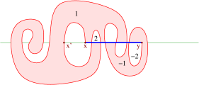
Figure 1: Maslov index and catenation: $x^{\prime}<x<y$.

By Step 2 we may assume ${\varepsilon}_{x}(\Lambda)=1$. Orient $B$ from $x$ to $y$. The Viterbo–Maslov index of $\Lambda$ is minus the Maslov index of the path $B\to{\mathbb{R}\mathrm{P}}^{1}:z\mapsto T_{z}B,$ relative to the Lagrangian subspace ${\mathbb{R}}\subset{\mathbb{C}}$. Since the Maslov index of the arc in $B$ from $x$ to $x^{\prime}$ is $+1$ we have

$$\mu(\Lambda)=\mu(\Lambda^{\prime})-1.$$ (11)

Since the orientations of $A^{\prime}$ and $B^{\prime}$ agree with those of $A$ and $B$ we have

$${\varepsilon}_{x^{\prime}}(\Lambda^{\prime})={\varepsilon}_{x^{\prime}}(\Lambda)=-1,\qquad{\varepsilon}_{y}(\Lambda^{\prime})={\varepsilon}_{y}(\Lambda).$$ (12)

Now let $x_{1}<x_{2}<\cdots<x_{m}<x$ be the intersection points of ${\mathbb{R}}$ and $B$ in the interval $(-\infty,x)$ and let ${\varepsilon}_{i}\in\{-1,+1\}$ be the intersection index of ${\mathbb{R}}$ and $B$ at $x_{i}$. Then there is an integer $\ell\in\{1,\dots,m\}$ such that $x_{\ell}=x^{\prime}$ and ${\varepsilon}_{\ell}=-1$. Moreover, the winding number ${\rm w}$ slightly to the left of $x$ is

$$k_{x}(\Lambda)=\sum_{i=1}^{m}{\varepsilon}_{i}.$$

It agrees with the value of ${\rm w}$ slightly to the right of $x^{\prime}=x_{\ell}$. Hence

$$k_{x}(\Lambda)=\sum_{i=1}^{\ell}{\varepsilon}_{i}=\sum_{i=1}^{\ell-1}{\varepsilon}_{i}-1=k_{x^{\prime}}(\Lambda^{\prime})-1,\qquad k_{y}(\Lambda^{\prime})=k_{y}(\Lambda).$$ (13)

It follows from equation (9) for $\Lambda^{\prime}$ and equations (11), (12), and (13) that

$$\mu(\Lambda) = \mu(\Lambda^{\prime})-1$$

$$= 2k_{x^{\prime}}(\Lambda^{\prime})+2k_{y}(\Lambda^{\prime})+\frac{{\varepsilon}_{x^{\prime}}(\Lambda^{\prime})-{\varepsilon}_{y}(\Lambda^{\prime})}{2}-1$$

$$= 2k_{x^{\prime}}(\Lambda^{\prime})+2k_{y}(\Lambda^{\prime})+\frac{-1-{\varepsilon}_{y}(\Lambda)}{2}-1$$

$$= 2k_{x^{\prime}}(\Lambda^{\prime})+2k_{y}(\Lambda^{\prime})+\frac{1-{\varepsilon}_{y}(\Lambda)}{2}-2$$

$$= 2k_{x}(\Lambda)+2k_{y}(\Lambda)+\frac{{\varepsilon}_{x}(\Lambda)-{\varepsilon}_{y}(\Lambda)}{2}.$$

This proves Step 4.

Step 5. Assume (10) and $\#(B\cap{\mathbb{R}})>2$, follow the arc of $B$, starting at $x$, and let $x^{\prime}$ be the next intersection point with ${\mathbb{R}}$. Assume $x<x^{\prime}<y$, denote by $B^{\prime}$ the arc in $B$ from $x^{\prime}$ to $y$, and let $A^{\prime}:=[x^{\prime},y]$ (see Figure 2). If the $(\alpha,\beta)$-trace $\Lambda^{\prime}$ with boundary ${\partial}\Lambda^{\prime}=(x^{\prime},y,A^{\prime},B^{\prime})$ satisfies (9) so does $\Lambda$.

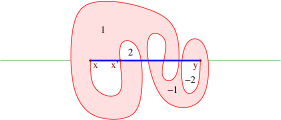
Figure 2: Maslov index and catenation: $x<x^{\prime}<y$.

By Step 2 we may assume ${\varepsilon}_{x}(\Lambda)=1$. Since the Maslov index of the arc in $B$ from $x$ to $x^{\prime}$ is $-1$, we have

$$\mu(\Lambda)=\mu(\Lambda^{\prime})+1.$$ (14)

Since the orientations of $A^{\prime}$ and $B^{\prime}$ agree with those of $A$ and $B$ we have

$${\varepsilon}_{x^{\prime}}(\Lambda^{\prime})={\varepsilon}_{x^{\prime}}(\Lambda)=-1,\qquad{\varepsilon}_{y}(\Lambda^{\prime})={\varepsilon}_{y}(\Lambda).$$ (15)

Now let $x<x_{1}<x_{2}<\cdots<x_{m}<x^{\prime}$ be the intersection points of ${\mathbb{R}}$ and $B$ in the interval $(x,x^{\prime})$ and let ${\varepsilon}_{i}\in\{-1,+1\}$ be the intersection index of ${\mathbb{R}}$ and $B$ at $x_{i}$. Since the interval $[x,x^{\prime}]$ in $A$ and the arc in $B$ from $x$ to $x^{\prime}$ bound an open half disc, every subarc of $B$ in this half disc must enter and exit through the open interval $(x,x^{\prime})$. Hence the intersections indices of ${\mathbb{R}}$ and $B$ at the points $x_{1},\dots,x_{m}$ cancel in pairs and thus

$$\sum_{i=1}^{m}{\varepsilon}_{i}=0.$$

Since $k_{x^{\prime}}(\Lambda^{\prime})$ is the sum of the intersection indices of ${\mathbb{R}}$ and $B^{\prime}$ at all points to the left of $x^{\prime}$ we obtain

$$k_{x^{\prime}}(\Lambda^{\prime})=k_{x}(\Lambda)+\sum_{i=1}^{m}{\varepsilon}_{i}=k_{x}(\Lambda),\qquad k_{y}(\Lambda^{\prime})=k_{y}(\Lambda).$$ (16)

It follows from equation (9) for $\Lambda^{\prime}$ and equations (14), (15), and (16) that

$$\mu(\Lambda) = \mu(\Lambda^{\prime})+1$$

$$= 2k_{x^{\prime}}(\Lambda^{\prime})+2k_{y}(\Lambda^{\prime})+\frac{{\varepsilon}_{x^{\prime}}(\Lambda^{\prime})-{\varepsilon}_{y}(\Lambda^{\prime})}{2}+1$$

$$= 2k_{x}(\Lambda)+2k_{y}(\Lambda)+\frac{-1-{\varepsilon}_{y}(\Lambda)}{2}+1$$

$$= 2k_{x}(\Lambda)+2k_{y}(\Lambda)+\frac{{\varepsilon}_{x}(\Lambda)-{\varepsilon}_{y}(\Lambda)}{2}.$$

This proves Step 5.

Step 6. Assume (10) and $\#(B\cap{\mathbb{R}})>2$, follow the arc of $B$, starting at $x$, and let $y^{\prime}$ be the next intersection point with ${\mathbb{R}}$. Assume $y^{\prime}>y$. Denote by $B^{\prime}$ the arc in $B$ from $y$ to $y^{\prime}$, and let $A^{\prime}:=[y,y^{\prime}]$ (see Figure 3). If the $(\alpha,\beta)$-trace $\Lambda^{\prime}$ with boundary ${\partial}\Lambda^{\prime}=(y,y^{\prime},A^{\prime},B^{\prime})$ satisfies (9) so does $\Lambda$.

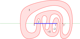
Figure 3: Maslov index and catenation: $x<y<y^{\prime}$.

By Step 2 we may assume ${\varepsilon}_{x}(\Lambda)=1$. Since the orientation of $B^{\prime}$ from $y$ to $y^{\prime}$ is opposite to the orientation of $B$ and the Maslov index of the arc in $B$ from $x$ to $y^{\prime}$ is $-1$, we have

$$\mu(\Lambda)=1-\mu(\Lambda^{\prime}).$$ (17)

Using again the fact that the orientation of $B^{\prime}$ is opposite to the orientation of $B$ we have

$${\varepsilon}_{y}(\Lambda^{\prime})=-{\varepsilon}_{y}(\Lambda),\qquad{\varepsilon}_{y^{\prime}}(\Lambda^{\prime})=-{\varepsilon}_{y^{\prime}}(\Lambda)=1.$$ (18)

Now let $x_{1}<x_{2}<\cdots<x_{m}$ be all intersection points of ${\mathbb{R}}$ and $B$ and let ${\varepsilon}_{i}\in\{-1,+1\}$ be the intersection index of ${\mathbb{R}}$ and $B$ at $x_{i}$. Choose

$$j<k<\ell$$

such that

$$x_{j}=x,\qquad x_{k}=y,\qquad x_{\ell}=y^{\prime}.$$

Then

$${\varepsilon}_{j}={\varepsilon}_{x}(\Lambda)=1,\qquad{\varepsilon}_{k}={\varepsilon}_{y}(\Lambda),\qquad{\varepsilon}_{\ell}={\varepsilon}_{y^{\prime}}(\Lambda)=-1,$$

and

$$k_{x}(\Lambda)=\sum_{i<j}{\varepsilon}_{i},\qquad k_{y}(\Lambda)=-\sum_{i>k}{\varepsilon}_{i}.$$

For $i\neq j$ the intersection index of ${\mathbb{R}}$ and $B^{\prime}$ at $x_{i}$ is $-{\varepsilon}_{i}$. Moreover, $k_{y}(\Lambda^{\prime})$ is the sum of the intersection indices of ${\mathbb{R}}$ and $B^{\prime}$ at all points to the left of $y$ and $k_{y^{\prime}}(\Lambda^{\prime})$ is minus the sum of the intersection indices of ${\mathbb{R}}$ and $B^{\prime}$ at all points to the right of $y^{\prime}$. Hence

$$k_{y}(\Lambda^{\prime})=-\sum_{i<j}{\varepsilon}_{i}-\sum_{j<i<k}{\varepsilon}_{i},\qquad k_{y^{\prime}}(\Lambda^{\prime})=\sum_{i>\ell}{\varepsilon}_{i}.$$

We claim that

$$k_{y^{\prime}}(\Lambda^{\prime})+k_{x}(\Lambda)=0,\qquad k_{y}(\Lambda^{\prime})+k_{y}(\Lambda)=\frac{1+{\varepsilon}_{y}(\Lambda)}{2}.$$ (19)

To see this, note that the value of the winding number ${\rm w}$ slightly to the left of $x$ agrees with the value of ${\rm w}$ slightly to the right of $y^{\prime}$, and hence

$$0=\sum_{i<j}{\varepsilon}_{i}+\sum_{i>\ell}{\varepsilon}_{i}=k_{x}(\Lambda)+k_{y^{\prime}}(\Lambda^{\prime}).$$

This proves the first equation in (19). To prove the second equation in (19) we observe that

$$\sum_{i=1}^{m}{\varepsilon}_{i}=\frac{{\varepsilon}_{x}(\Lambda)+{\varepsilon}_{y}(\Lambda)}{2}$$

and hence

$$k_{y}(\Lambda^{\prime})+k_{y}(\Lambda) = -\sum_{i<j}{\varepsilon}_{i}-\sum_{j<i<k}{\varepsilon}_{i}-\sum_{i>k}{\varepsilon}_{i}$$

$$= {\varepsilon}_{j}+{\varepsilon}_{k}-\sum_{i=1}^{m}{\varepsilon}_{i}$$

$$= {\varepsilon}_{x}(\Lambda)+{\varepsilon}_{y}(\Lambda)-\sum_{i=1}^{m}{\varepsilon}_{i}$$

$$= \frac{{\varepsilon}_{x}(\Lambda)+{\varepsilon}_{y}(\Lambda)}{2}$$

$$= \frac{1+{\varepsilon}_{y}(\Lambda)}{2}.$$

This proves the second equation in (19).

It follows from equation (9) for $\Lambda^{\prime}$ and equations (17), (18), and (19) that

$$\mu(\Lambda) = 1-\mu(\Lambda^{\prime})$$

$$= 1-2k_{y}(\Lambda^{\prime})-2k_{y^{\prime}}(\Lambda^{\prime})-\frac{{\varepsilon}_{y}(\Lambda^{\prime})-{\varepsilon}_{y^{\prime}}(\Lambda^{\prime})}{2}$$

$$= 1-2k_{y}(\Lambda^{\prime})-2k_{y^{\prime}}(\Lambda^{\prime})-\frac{-{\varepsilon}_{y}(\Lambda)-1}{2}$$

$$= 2k_{y}(\Lambda)-{\varepsilon}_{y}(\Lambda)+2k_{x}(\Lambda)+\frac{1+{\varepsilon}_{y}(\Lambda)}{2}$$

$$= 2k_{x}(\Lambda)+2k_{y}(\Lambda)+\frac{1-{\varepsilon}_{y}(\Lambda)}{2}.$$

Here the first equality follows from (17), the second equality follows from (9) for $\Lambda^{\prime}$, the third equality follows from (18), and the fourth equality follows from (19). This proves Step 6.

Step 7. The trace formula (7) holds when $\Sigma={\mathbb{C}}$ and $\Lambda$ satisfies the arc condition.

It follows from Steps 3-6 by induction that equation (9) holds for every $(\alpha,\beta)$-trace $\Lambda=(x,y,{\rm w})$ whose boundary ${\partial}\Lambda=(x,y,A,B)$ satisfies (10). Hence Step 7 follows from Step 1.

Next we drop the hypothesis that $\Lambda$ satisfies the arc condition and extend the result to planar surfaces. This requires a further three steps.

Step 8. The trace formula (7) holds when $\Sigma={\mathbb{C}}$ and $x=y$.

Under these hypotheses $\nu_{\alpha}:={\partial}{\rm w}|_{\alpha\setminus\beta}$ and $\nu_{\beta}:=-{\partial}{\rm w}|_{\beta\setminus\alpha}$ are constant. There are four cases.

Case 1. $\alpha$ is an embedded circle and $\beta$ is not an embedded circle. In this case we have $\nu_{\beta}\equiv 0$ and $B=\{x\}$. Moroeover, $\alpha$ is the boundary of a unique disc $\Delta_{\alpha}$ and we assume that $\alpha$ is oriented as the boundary of $\Delta_{\alpha}$. Then the path $\gamma_{\alpha}:[0,1]\to\Sigma$ in Definition 2.1 satisfies $\gamma_{\alpha}(0)=\gamma_{\alpha}(1)=x$ and is homotopic to $\nu_{\alpha}\alpha$. Hence

$$m_{x}(\Lambda)=m_{y}(\Lambda)=2\nu_{\alpha}=\mu(\Lambda).$$

Here the last equation follows from the fact that $\Lambda$ can be obtained as the catenation of $\nu_{\alpha}$ copies of the disc $\Delta_{\alpha}$.

Case 2. $\alpha$ is not an embedded circle and $\beta$ is an embedded circle. This follows from Case 1 by interchanging $\alpha$ and $\beta$.

Case 3. $\alpha$ and $\beta$ are embedded circles. In this case there is a unique pair of embedded discs $\Delta_{\alpha}$ and $\Delta_{\beta}$ with boundaries $\alpha$ and $\beta$, respectively. Orient $\alpha$ and $\beta$ as the boundaries of these discs. Then, for every $z\in\Sigma\setminus\alpha\cup\beta$, we have

$${\rm w}(z)=\left\{\begin{array}[]{ll}\nu_{\alpha}-\nu_{\beta},&\mbox{for }z\in\Delta_{\alpha}\cap\Delta_{\beta},\\ \nu_{\alpha},&\mbox{for }z\in\Delta_{\alpha}\setminus\overline{\Delta}_{\beta},\\ -\nu_{\beta},&\mbox{for }z\in\Delta_{\beta}\setminus\overline{\Delta}_{\alpha},\\ 0,&\mbox{for }z\in\Sigma\setminus\overline{\Delta}_{\alpha}\cup\overline{\Delta}_{\beta}.\end{array}\right.$$

Hence

$$m_{x}(\Lambda)=m_{y}(\Lambda)=2\nu_{\alpha}-2\nu_{\beta}=\mu(\Lambda).$$

Here the last equation follows from the fact $\Lambda$ can be obtained as the catenation of $\nu_{\alpha}$ copies of the disc $\Delta_{\alpha}$ (with the orientation inherited from $\Sigma$) and $\nu_{\beta}$ copies of $-\Delta_{\beta}$ (with the opposite orientation).

Case 4. Neither $\alpha$ nor $\beta$ is an embedded circle. Under this hypothesis we have $\nu_{\alpha}=\nu_{\beta}=0$. Hence it follows from Theorem 2.4 that ${\rm w}=0$ and $\Lambda=\Lambda_{u}$ for the constant map $u\equiv x\in{\mathcal{D}}(x,x)$. Thus

$$m_{x}(\Lambda)=m_{y}(\Lambda)=\mu(\Lambda)=0.$$

This proves Step 8.

Step 9. The trace formula (7) holds when $\Sigma={\mathbb{C}}$.

By Step 8, it suffices to assume $x\neq y$. It follows from Theorem 2.4 that every $u\in{\mathcal{D}}(x,y)$ is homotopic to a catentation $u=u_{0}\#v$, where $u_{0}\in{\mathcal{D}}(x,y)$ satisfies the arc condition and $v\in{\mathcal{D}}(y,y)$. Hence it follows from Steps 7 and 8 that

$$\mu(\Lambda_{u}) = \mu(\Lambda_{u_{0}})+\mu(\Lambda_{v})$$

$$= \frac{m_{x}(\Lambda_{u_{0}})+m_{y}(\Lambda_{u_{0}})}{2}+m_{y}(\Lambda_{v})$$

$$= \frac{m_{x}(\Lambda_{u})+m_{y}(\Lambda_{u})}{2}.$$

Here the last equation follows from the fact that ${\rm w}_{u}={\rm w}_{u_{0}}+{\rm w}_{v}$ and hence $m_{z}(\Lambda_{u})=m_{z}(\Lambda_{u_{0}})+m_{z}(\Lambda_{v})$ for every $z\in\alpha\cap\beta$. This proves Step 9.

Step 10. The trace formula (7) holds when $\Sigma$ is planar.

Choose an element $u\in{\mathcal{D}}(x,y)$ such that $\Lambda_{u}=\Lambda$. Modifying $\alpha$ and $\beta$ on the complement of $u({\mathbb{D}})$, if necessary, we may assume without loss of generality that $\alpha$ and $\beta$ are embedded circles. Let $\iota:\Sigma\to{\mathbb{C}}$ be an orientation preserving embedding. Then $\iota_{*}\Lambda:=\Lambda_{\iota\circ u}$ is an $(\iota(\alpha),\iota(\beta))$-trace in ${\mathbb{C}}$ and hence satisfies the trace formula (7) by Step 9. Since $m_{\iota(x)}(\iota_{*}\Lambda)=m_{x}(\Lambda)$, $m_{\iota(y)}(\iota_{*}\Lambda)=m_{y}(\Lambda)$, and $\mu(\iota_{*}\Lambda)=\mu(\Lambda)$ it follows that $\Lambda$ also satisfies the trace formula. This proves Step 10 and Proposition 4.1 ∎

Remark 4.2.

Let $\Lambda=(x,y,A,B)$ be an $(\alpha,\beta)$-trace in ${\mathbb{C}}$ as in Step 1 in the proof of Theorem 3.4. Thus $x<y$ are real numbers, $A$ is the interval $[x,y]$, and $B$ is an embedded arc with endpoints $x,y$ which is oriented from $x$ to $y$ and is transverse to ${\mathbb{R}}$. Thus $Z:=B\cap{\mathbb{R}}$ is a finite set. Define a map

$$f:Z\setminus\{y\}\to Z\setminus\{x\}$$

as follows. Given $z\in Z\setminus\{y\}$ walk along $B$ towards $y$ and let $f(z)$ be the next intersection point with ${\mathbb{R}}$. This map is bijective. Now let $I$ be any of the three open intervals $(-\infty,x)$, $(x,y)$, $(y,\infty)$. Any arc in $B$ from $z$ to $f(z)$ with both endpoints in the same interval $I$ can be removed by an isotopy of $B$ which does not pass through $x,y$. Call $\Lambda$ a reduced $(\alpha,\beta)$-trace if $z\in I$ implies $f(z)\notin I$ for each of the three intervals. Then every $(\alpha,\beta)$-trace is isotopic to a reduced $(\alpha,\beta^{\prime})$-trace and the isotopy does not affect the numbers $\mu,k_{x},k_{y},{\varepsilon}_{x},{\varepsilon}_{y}$.

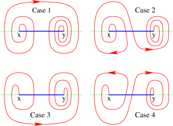
Figure 4: Reduced $(\alpha,\beta)$-traces in ${\mathbb{C}}$.

Let $Z^{+}$ (respectively $Z^{-}$) denote the set of all points $z\in Z=B\cap{\mathbb{R}}$ where the positive tangent vectors in $T_{z}B$ point up (respectively down). One can prove that every reduced $(\alpha,\beta)$-trace satisfies one of the following conditions.

Case 1: If $z\in Z^{+}\setminus\{y\}$ then $f(z)>z$.  Case 2: $Z^{-}\subset[x,y]$.

Case 3: If $z\in Z^{-}\setminus\{y\}$ then $f(z)>z$.  Case 4: $Z^{+}\subset[x,y]$.

(Examples with ${\varepsilon}_{x}=1$ and ${\varepsilon}_{y}=-1$ are depicted in Figure 4.) One can then show directly that the reduced $(\alpha,\beta)$-traces satisfy equation (9). This gives rise to an alternative proof of Proposition 4.1 via case distinction.

Proof of Theorem 3.4 in the Simply Connected Case.

If $\Sigma$ is diffeomorphic to the $2$-plane the result has been established in Proposition 4.1. Hence assume

$$\Sigma=S^{2}.$$

Let $u\in{\mathcal{D}}(x,y)$. If $u$ is not surjective the assertion follows from the case of the complex plane (Proposition 4.1) via stereographic projection. Hence assume $u$ is surjective and choose a regular value $z\in S^{2}\setminus(\alpha\cup\beta)$ of $u$. Denote

$$u^{-1}(z)=\{z_{1},\dots,z_{k}\}.$$

For $i=1,\dots,k$ let ${\varepsilon}_{i}=\pm 1$ according to whether or not the differential $du(z_{i}):{\mathbb{C}}\to T_{z}\Sigma$ is orientation preserving. Choose an open disc $\Delta\subset S^{2}$ centered at $z$ such that

$$\bar{\Delta}\cap(\alpha\cup\beta)=\emptyset$$

and $u^{-1}(\Delta)$ is a union of open neighborhoods $U_{i}\subset{\mathbb{D}}$ of $z_{i}$ with disjoint closures such that

$$u|_{U_{i}}:U_{i}\to\Delta$$

is a diffeomorphism for each $i$ which extends to a neighborhood of $\bar{U}_{i}$. Now choose a continuous map $u^{\prime}:{\mathbb{D}}\to S^{2}$ which agrees with $u$ on ${\mathbb{D}}\setminus\bigcup_{i}U_{i}$ and restricts to a diffeomorphism from $\bar{U}_{i}$ to $S^{2}\setminus\Delta$ for each $i$. Then $z$ does not belong to the image of $u^{\prime}$ and hence the trace formula (7) holds for $u^{\prime}$ (after smoothing along the boundaries ${\partial}U_{i}$). Moreover, the diffeomorphism

$$u^{\prime}|_{\bar{U}_{i}}:\bar{U}_{i}\to S^{2}\setminus\Delta$$

is orientation preserving if and only if ${\varepsilon}_{i}=-1$. Hence

$$\begin{split}\mu(\Lambda_{u})&=\mu(\Lambda_{u^{\prime}})+4\sum_{i=1}^{k}{\varepsilon}_{i},\\ m_{x}(\Lambda_{u})&=m_{x}(\Lambda_{u^{\prime}})+4\sum_{i=1}^{k}{\varepsilon}_{i},\\ m_{y}(\Lambda_{u})&=m_{y}(\Lambda_{u^{\prime}})+4\sum_{i=1}^{k}{\varepsilon}_{i}.\end{split}$$

By Proposition 4.1 the trace formula (7) holds for $\Lambda_{u^{\prime}}$ and hence it also holds for $\Lambda_{u}$. This proves Theorem 3.4 when $\Sigma$ is simply connected. ∎

5 The Non Simply Connected Case

The key step for extending Proposition 4.1 to non-simply connected two-manifolds is the next result about lifts to the universal cover.

Proposition 5.1.

Suppose $\Sigma$ is not diffeomorphic to the $2$-sphere. Let ${\Lambda=(x,y,{\rm w})}$ be an $(\alpha,\beta)$-trace and ${\pi:{\mathbb{C}}\to\Sigma}$ be a universal covering. Denote by $\Gamma\subset{\rm Diff}({\mathbb{C}})$ the group of deck transformations. Choose an element ${{\widetilde{x}}\in\pi^{-1}(x)}$ and let ${\widetilde{\alpha}}$ and ${\widetilde{\beta}}$ be the lifts of $\alpha$ and $\beta$ through ${\widetilde{x}}$. Let ${\widetilde{\Lambda}}=({\widetilde{x}},{\widetilde{y}},\widetilde{\rm w})$ be the lift of $\Lambda$ with left endpoint ${\widetilde{x}}$. Then ${\widetilde{\Lambda}}$ satisfies the cancellation formula

$$m_{g{\widetilde{x}}}({\widetilde{\Lambda}})+m_{g^{-1}{\widetilde{y}}}({\widetilde{\Lambda}})=0$$ (20)

for every $g\in\Gamma\setminus\{{\rm id}\}$. (Proof on page 5.)

Lemma 5.2 (Annulus Reduction).

Suppose $\Sigma$ is not diffeomorphic to the $2$-sphere. Let $\Lambda$, $\pi$, $\Gamma$, ${\widetilde{\Lambda}}$ be as in Proposition 5.1. If

$$m_{g{\widetilde{x}}}({\widetilde{\Lambda}})+m_{g^{-1}{\widetilde{y}}}({\widetilde{\Lambda}})=m_{g^{-1}{\widetilde{x}}}({\widetilde{\Lambda}})+m_{g{\widetilde{y}}}({\widetilde{\Lambda}})$$ (21)

for all $g\in\Gamma\setminus\{{\rm id}\}$ then the cancellation formula (20) holds for all $g\in\Gamma\setminus\{{\rm id}\}$.

Proof.

If (20) does not hold then there is a deck transformation $h\in\Gamma\setminus\{{\rm id}\}$ such that $m_{h{\widetilde{x}}}({\widetilde{\Lambda}})+m_{h^{-1}{\widetilde{y}}}({\widetilde{\Lambda}})\neq 0.$ Since there can only be finitely many such $h\in\Gamma\setminus\{{\rm id}\}$, there is an integer $k\geq 1$ such that $m_{h^{k}{\widetilde{x}}}({\widetilde{\Lambda}})+m_{h^{-k}{\widetilde{y}}}({\widetilde{\Lambda}})\neq 0$ and $m_{h^{\ell}{\widetilde{x}}}({\widetilde{\Lambda}})+m_{h^{-\ell}{\widetilde{y}}}({\widetilde{\Lambda}})=0$ for every integer $\ell>k$. Define $g:=h^{k}$. Then

$$m_{g{\widetilde{x}}}({\widetilde{\Lambda}})+m_{g^{-1}{\widetilde{y}}}({\widetilde{\Lambda}})\neq 0$$ (22)

and $m_{g^{k}{\widetilde{x}}}({\widetilde{\Lambda}})+m_{g^{-k}{\widetilde{y}}}({\widetilde{\Lambda}})=0$ for every integer $k\in{\mathbb{Z}}\setminus\{-1,0,1\}$. Define

$$\Sigma_{0}:={\mathbb{C}}/\Gamma_{0},\qquad\Gamma_{0}:=\left\{g^{k}\,|\,k\in{\mathbb{Z}}\right\}.$$

Then $\Sigma_{0}$ is diffeomorphic to the annulus. Let $\pi_{0}:{\mathbb{C}}\to\Sigma_{0}$ be the obvious projection, define $\alpha_{0}:=\pi_{0}({\widetilde{\alpha}})$, $\beta_{0}:=\pi_{0}({\widetilde{\beta}})$, and let $\Lambda_{0}:=(x_{0},y_{0},{\rm w}_{0})$ be the $(\alpha_{0},\beta_{0})$-trace in $\Sigma_{0}$ with $x_{0}:=\pi_{0}({\widetilde{x}})$, $y_{0}:=\pi_{0}({\widetilde{y}})$, and

$${\rm w}_{0}(z_{0}):=\sum_{{\widetilde{z}}\in\pi_{0}^{-1}(z_{0})}\widetilde{\rm w}({\widetilde{z}}),\qquad z_{0}\in\Sigma_{0}\setminus(\alpha_{0}\cup\beta_{0}).$$

Then

$$\begin{split}m_{x_{0}}(\Lambda_{0})&=m_{\widetilde{x}}({\widetilde{\Lambda}})+\sum_{k\in{\mathbb{Z}}\setminus\{0\}}m_{g^{k}{\widetilde{x}}}({\widetilde{\Lambda}}),\\ m_{y_{0}}(\Lambda_{0})&=m_{\widetilde{y}}({\widetilde{\Lambda}})+\sum_{k\in{\mathbb{Z}}\setminus\{0\}}m_{g^{-k}{\widetilde{y}}}({\widetilde{\Lambda}}).\end{split}$$

By Proposition 4.1 both ${\widetilde{\Lambda}}$ and $\Lambda_{0}$ satisfy the trace formula (7) and they have the same Viterbo–Maslov index. Hence

$$0 = \mu(\Lambda_{0})-\mu({\widetilde{\Lambda}})$$

$$= \frac{m_{x_{0}}(\Lambda_{0})+m_{y_{0}}(\Lambda_{0})}{2}-\frac{m_{\widetilde{x}}({\widetilde{\Lambda}})+m_{\widetilde{y}}({\widetilde{\Lambda}})}{2}$$

$$= \frac{1}{2}\sum_{k\neq 0}\left(m_{g^{k}{\widetilde{x}}}({\widetilde{\Lambda}})+m_{g^{-k}{\widetilde{y}}}({\widetilde{\Lambda}})\right)$$

$$= m_{g{\widetilde{x}}}({\widetilde{\Lambda}})+m_{g^{-1}{\widetilde{y}}}({\widetilde{\Lambda}}).$$

Here the last equation follows from (21). This contradicts (22) and proves Lemma 5.2. ∎

Lemma 5.3.

Suppose $\Sigma$ is not diffeomorphic to the $2$-sphere. Let $\Lambda$, $\pi$, $\Gamma$, ${\widetilde{\Lambda}}$ be as in Proposition 5.1 and denote $\nu_{\widetilde{\alpha}}:={\partial}\widetilde{\rm w}|_{{\widetilde{\alpha}}\setminus{\widetilde{\beta}}}$ and $\nu_{\widetilde{\beta}}:=-{\partial}\widetilde{\rm w}|_{{\widetilde{\beta}}\setminus{\widetilde{\alpha}}}$. Choose smooth paths

$$\gamma_{\widetilde{\alpha}}:[0,1]\to{\widetilde{\alpha}},\qquad\gamma_{\widetilde{\beta}}:[0,1]\to{\widetilde{\beta}}$$

from $\gamma_{\widetilde{\alpha}}(0)=\gamma_{\widetilde{\beta}}(0)={\widetilde{x}}$ to $\gamma_{\widetilde{\alpha}}(1)=\gamma_{\widetilde{\beta}}(1)={\widetilde{y}}$ such that $\gamma_{\widetilde{\alpha}}$ is an immersion when $\nu_{\widetilde{\alpha}}\not\equiv 0$ and constant when $\nu_{\widetilde{\alpha}}\equiv 0$, the same holds for $\gamma_{\widetilde{\beta}}$, and

$$\begin{split}\nu_{\widetilde{\alpha}}({\widetilde{z}})=\deg(\gamma_{\widetilde{\alpha}},{\widetilde{z}})&\quad\mbox{for}\quad{\widetilde{z}}\in{\widetilde{\alpha}}\setminus\{{\widetilde{x}},{\widetilde{y}}\},\\ \nu_{\widetilde{\beta}}({\widetilde{z}})=\deg(\gamma_{\widetilde{\beta}},{\widetilde{z}})&\quad\mbox{for}\quad{\widetilde{z}}\in{\widetilde{\beta}}\setminus\{{\widetilde{x}},{\widetilde{y}}\}.\end{split}$$

Define

$${\widetilde{A}}:=\gamma_{\widetilde{\alpha}}([0,1]),\qquad{\widetilde{B}}:=\gamma_{\widetilde{\beta}}([0,1]).$$

Then, for every $g\in\Gamma$, we have

$$g{\widetilde{x}}\in{\widetilde{A}}\qquad\iff\qquad g^{-1}{\widetilde{y}}\in{\widetilde{A}},$$ (23)

$$g{\widetilde{x}}\notin{\widetilde{A}}\;\;\mbox{ and }\;\;g{\widetilde{y}}\notin{\widetilde{A}}\qquad\iff\qquad{\widetilde{A}}\cap g{\widetilde{A}}=\emptyset,$$ (24)

$$g{\widetilde{x}}\in{\widetilde{A}}\;\;\mbox{ and }\;\;g{\widetilde{y}}\in{\widetilde{A}}\qquad\iff\qquad g={\rm id}.$$ (25)

The same holds with ${\widetilde{A}}$ replaced by ${\widetilde{B}}$.

Proof.

If $\alpha$ is a contractible embedded circle or not an embedded circle at all we have ${\widetilde{A}}\cap g{\widetilde{A}}=\emptyset$ whenever $g\neq{\rm id}$ and this implies (23), (24) and (25). Hence assume $\alpha$ is a noncontractible embedded circle. Then we may also assume, without loss of generality, that $\pi({\mathbb{R}})=\alpha$, the map ${\widetilde{z}}\mapsto{\widetilde{z}}+1$ is a deck transformation, $\pi$ maps the interval $[0,1)$ bijectively onto $\alpha$, and ${\widetilde{x}},{\widetilde{y}}\in{\mathbb{R}}={\widetilde{\alpha}}$ with ${\widetilde{x}}<{\widetilde{y}}$. Thus ${\widetilde{A}}=[{\widetilde{x}},{\widetilde{y}}]$ and, for every $k\in{\mathbb{Z}}$,

$${\widetilde{x}}+k\in[{\widetilde{x}},{\widetilde{y}}]\quad\iff\quad 0\leq k\leq{\widetilde{y}}-{\widetilde{x}}\quad\iff\quad{\widetilde{y}}-k\in[{\widetilde{x}},{\widetilde{y}}].$$

Similarly, we have

$${\widetilde{x}}+k,{\widetilde{y}}+k\notin[{\widetilde{x}},{\widetilde{y}}]\quad\iff\quad[{\widetilde{x}}+k,{\widetilde{y}}+k]\cap[{\widetilde{x}},{\widetilde{y}}]=\emptyset$$

and

$${\widetilde{x}}+k,{\widetilde{y}}+k\in[{\widetilde{x}},{\widetilde{y}}]\quad\iff\quad[{\widetilde{x}}+k,{\widetilde{y}}+k]\subset[{\widetilde{x}},{\widetilde{y}}]\quad\iff\quad k=0.$$

This proves (23), (24), and (25) for the deck transformation ${\widetilde{z}}\mapsto{\widetilde{z}}+k$. If $g$ is any other deck transformation, then we have ${\widetilde{\alpha}}\cap g{\widetilde{\alpha}}=\emptyset$ and so (23), (24), and (25) are trivially satisfied. This proves Lemma 5.3. ∎

Lemma 5.4 (Winding Number Comparison).

Suppose $\Sigma$ is not diffeomorphic to the $2$-sphere. Let $\Lambda$, $\pi$, $\Gamma$, ${\widetilde{\Lambda}}$ be as in Proposition 5.1, and let ${\widetilde{A}},{\widetilde{B}}\subset{\mathbb{C}}$ be as in Lemma 5.3. Then the following holds.

(i) Equation (21) holds for every $g\in\Gamma$ that satisfies $g{\widetilde{x}},g{\widetilde{y}}\notin{\widetilde{A}}\cup{\widetilde{B}}$.

(ii) If $\Lambda$ satisfies the arc condition then it also satisfies the cancellation formula (20) for every $g\in\Gamma\setminus\{{\rm id}\}$.

Proof.

We prove (i). Let $g\in\Gamma$ such that $g{\widetilde{x}},g{\widetilde{y}}\notin{\widetilde{A}}\cup{\widetilde{B}}$ and let $\gamma_{\widetilde{\alpha}},\gamma_{\widetilde{\beta}}$ be as in Lemma 5.3. Then $\widetilde{\rm w}({\widetilde{z}})$ is the winding number of the loop $\gamma_{\widetilde{\alpha}}-\gamma_{\widetilde{\beta}}$ about the point ${\widetilde{z}}\in{\mathbb{C}}\setminus({\widetilde{A}}\cup{\widetilde{B}})$. Moreover, the paths $g\gamma_{\widetilde{\alpha}},g\gamma_{\widetilde{\beta}}:[0,1]\to{\mathbb{C}}$ connect the points $g{\widetilde{x}},g{\widetilde{y}}\in{\mathbb{C}}\setminus({\widetilde{A}}\cup{\widetilde{B}})$. Hence

$$\widetilde{\rm w}(g{\widetilde{y}})-\widetilde{\rm w}(g{\widetilde{x}})=(\gamma_{\widetilde{\alpha}}-\gamma_{\widetilde{\beta}})\cdot g\gamma_{\widetilde{\alpha}}=(\gamma_{\widetilde{\alpha}}-\gamma_{\widetilde{\beta}})\cdot g\gamma_{\widetilde{\beta}}.$$

Similarly with $g$ replaced by $g^{-1}$. Moreover, it follows from Lemma 5.3, that

$${\widetilde{A}}\cap g{\widetilde{A}}=\emptyset,\qquad{\widetilde{B}}\cap g^{-1}{\widetilde{B}}=\emptyset.$$

Hence

$$\widetilde{\rm w}(g{\widetilde{y}})-\widetilde{\rm w}(g{\widetilde{x}}) = \left(\gamma_{\widetilde{\alpha}}-\gamma_{\widetilde{\beta}}\right)\cdot g\gamma_{\widetilde{\alpha}}$$

$$= g\gamma_{\widetilde{\alpha}}\cdot\gamma_{\widetilde{\beta}}$$

$$= \gamma_{\widetilde{\alpha}}\cdot g^{-1}\gamma_{\widetilde{\beta}}$$

$$= \left(\gamma_{\widetilde{\alpha}}-\gamma_{\widetilde{\beta}}\right)\cdot g^{-1}\gamma_{\widetilde{\beta}}$$

$$= \widetilde{\rm w}(g^{-1}{\widetilde{y}})-\widetilde{\rm w}(g^{-1}{\widetilde{x}})$$

Here we have used the fact that every $g\in\Gamma$ is an orientation preserving diffeomorphism of ${\mathbb{C}}$. Thus we have proved that

$$\widetilde{\rm w}(g{\widetilde{x}})+\widetilde{\rm w}(g^{-1}{\widetilde{y}})=\widetilde{\rm w}(g{\widetilde{y}})+\widetilde{\rm w}(g^{-1}{\widetilde{x}}).$$

Since $g{\widetilde{x}},g{\widetilde{y}}\notin{\widetilde{A}}\cup{\widetilde{B}}$, we have

$$m_{g{\widetilde{x}}}({\widetilde{\Lambda}})=4\widetilde{\rm w}(g{\widetilde{x}}),\qquad m_{g^{-1}{\widetilde{y}}}({\widetilde{\Lambda}})=4\widetilde{\rm w}(g^{-1}{\widetilde{y}}),$$

and the same identities hold with $g$ replaced by $g^{-1}$. This proves (i).

We prove (ii). If $\Lambda$ satisfies the arc condition then $g{\widetilde{A}}\cap{\widetilde{A}}=\emptyset$ and $g{\widetilde{B}}\cap{\widetilde{B}}=\emptyset$ for every $g\in\Gamma\setminus\{{\rm id}\}$. In particular, for every $g\in\Gamma\setminus\{{\rm id}\}$, we have $g{\widetilde{x}},g{\widetilde{y}}\notin{\widetilde{A}}\cup{\widetilde{B}}$ and hence (21) holds by (i). Hence it follows from Lemma 5.2 that the cancellation formula (20) holds for every $g\in\Gamma\setminus\{{\rm id}\}$. This proves Lemma 5.4. ∎

The next lemma deals with $(\alpha,\beta)$-traces connecting a point $x\in\alpha\cap\beta$ to itself. An example on the annulus is depicted in Figure 5.

Lemma 5.5 (Isotopy Argument).

Suppose $\Sigma$ is not diffeomorphic to the $2$-sphere. Let $\Lambda$, $\pi$, $\Gamma$, ${\widetilde{\Lambda}}$ be as in Proposition 5.1. Suppose that there is a deck transformation $g_{0}\in\Gamma\setminus\{{\rm id}\}$ such that ${\widetilde{y}}=g_{0}{\widetilde{x}}$. Then $\Lambda$ has Viterbo–Maslov index zero and $m_{g{\widetilde{x}}}({\widetilde{\Lambda}})=0$ for every $g\in\Gamma\setminus\{{\rm id},g_{0}\}$.

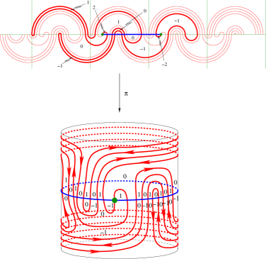
Figure 5: An $(\alpha,\beta)$-trace on the annulus with $x=y$.

Proof.

By hypothesis, we have ${\widetilde{\alpha}}=g_{0}{\widetilde{\alpha}}$ and ${\widetilde{\beta}}=g_{0}{\widetilde{\beta}}$. Hence $\alpha$ and $\beta$ are noncontractible embedded circles and some iterate of $\alpha$ is homotopic to some iterate of $\beta$. Hence, by Lemma A.4, $\alpha$ must be homotopic to $\beta$ (with some orientation). Hence we may assume, without loss of generality, that $\pi({\mathbb{R}})=\alpha$, the map ${\widetilde{z}}\mapsto{\widetilde{z}}+1$ is a deck transformation, $\pi$ maps the interval $[0,1)$ bijectively onto $\alpha$, ${\mathbb{R}}={\widetilde{\alpha}}$, ${\widetilde{x}}=0\in{\widetilde{\alpha}}\cap{\widetilde{\beta}}$, ${\widetilde{\beta}}={\widetilde{\beta}}+1$, and that ${\widetilde{y}}=\ell>0$ is an integer. Then $g_{0}$ is the translation

$$g_{0}({\widetilde{z}})={\widetilde{z}}+\ell.$$

Let ${\widetilde{A}}:=[0,\ell]\subset{\widetilde{\alpha}}$ and let ${\widetilde{B}}\subset{\widetilde{\beta}}$ be the arc connecting $0$ to $\ell$. Then, for ${\widetilde{z}}\in{\mathbb{C}}\setminus({\widetilde{A}}\cup{\widetilde{B}})$, the integer $\widetilde{\rm w}({\widetilde{z}})$ is the winding number of ${\widetilde{A}}-{\widetilde{B}}$ about ${\widetilde{z}}$. Define the projection $\pi_{0}:{\mathbb{C}}\to{\mathbb{C}}$ by

$$\pi_{0}({\widetilde{z}}):=e^{2\pi{\mathbf{i}}{\widetilde{z}}/\ell},$$

denote $\alpha_{0}:=\pi_{0}({\widetilde{\alpha}})=S^{1}$ and $\beta_{0}:=\pi({\widetilde{\beta}})$, and let $\Lambda_{0}=(1,1,{\rm w}_{0})$ be the induced $(\alpha_{0},\beta_{0})$-trace in ${\mathbb{C}}$ with ${\rm w}_{0}(z):=\sum_{{\widetilde{z}}\in\pi^{-1}(z)}\widetilde{\rm w}({\widetilde{z}})$. Then $\Lambda_{0}$ satisfies the conditions of Step 8, Case 3 in the proof of Proposition 4.1 and its boundary is given by $\nu_{\alpha_{0}}={\partial}{\rm w}_{0}|_{\alpha_{0}\setminus\beta_{0}}\equiv 1$ and $\nu_{\beta_{0}}={\partial}{\rm w}_{0}|_{\beta_{0}\setminus\alpha_{0}}\equiv 1$. Hence $\Lambda_{0}$ and ${\widetilde{\Lambda}}$ have Viterbo–Maslov index zero.

It remains to prove that $m_{g{\widetilde{x}}}({\widetilde{\Lambda}})=0$ for every $g\in\Gamma\setminus\{{\rm id},g_{0}\}$. To see this we use the fact that the embedded loops $\alpha$ and $\beta$ are homotopic with fixed endpoint $x$. Hence, by a Theorem of Epstein, they are isotopic with fixed basepoint $x$ (see [8, Theorem 4.1]). Thus there exists a smooth map $f:{\mathbb{R}}/{\mathbb{Z}}\times[0,1]\to\Sigma$ such that

$$f(s,0)\in\alpha,\qquad f(s,1)\in\beta,\qquad f(0,t)=x,$$

for all $s\in{\mathbb{R}}/{\mathbb{Z}}$ and $t\in[0,1]$, and the map ${\mathbb{R}}/{\mathbb{Z}}\to\Sigma:s\mapsto f(s,t)$ is an embedding for every $t\in[0,1]$. Lift this homotopy to the universal cover to obtain a map ${\widetilde{f}}:{\mathbb{R}}\times[0,1]\to{\mathbb{C}}$ such that $\pi\circ{\widetilde{f}}=f$ and

$${\widetilde{f}}(s,0)\in[0,1],\quad{\widetilde{f}}(s,1)\in{\widetilde{B}}_{1},\quad{\widetilde{f}}(0,t)={\widetilde{x}},\quad{\widetilde{f}}(s+k,t)={\widetilde{f}}(s,t)+k$$

for all $s,t\in[0,1]$ and $k\in{\mathbb{Z}}$. Here ${\widetilde{B}}_{1}\subset{\widetilde{B}}$ denotes the arc in ${\widetilde{B}}$ from $0$ to $1$. Since the map ${\mathbb{R}}/{\mathbb{Z}}\to\Sigma:s\mapsto f(s,t)$ is injective for every $t$, we have

$$g{\widetilde{x}}\notin\{{\widetilde{x}},{\widetilde{x}}+1,\dots,{\widetilde{x}}+\ell\}\qquad\implies\qquad g{\widetilde{x}}\notin{\widetilde{f}}([0,\ell]\times[0,1])$$

for every every $g\in\Gamma$. Now choose a smooth map ${\widetilde{u}}:{\mathbb{D}}\to{\mathbb{C}}$ with $\Lambda_{\widetilde{u}}={\widetilde{\Lambda}}$ (see Theorem 2.4). Define the homotopy $F_{\widetilde{u}}:[0,\ell]\times[0,1]\to{\mathbb{C}}$ by $F_{\widetilde{u}}(s,t):={\widetilde{u}}(-\cos(\pi s/\ell),t\sin(\pi s/\ell))$. Then, by Theorem 2.4, $F_{\widetilde{u}}$ is homotopic to ${\widetilde{f}}|_{[0,\ell]\times[0,1]}$ subject to the boundary conditions ${\widetilde{f}}(s,0)\in{\widetilde{\alpha}}={\mathbb{R}}$, ${\widetilde{f}}(s,1)\in{\widetilde{\beta}}$, ${\widetilde{f}}(0,t)={\widetilde{x}}$, ${\widetilde{f}}(\ell,t)={\widetilde{y}}$. Hence, for every ${\widetilde{z}}\in{\mathbb{C}}\setminus({\widetilde{\alpha}}\cup{\widetilde{\beta}})$, we have

$$\widetilde{\rm w}({\widetilde{z}})=\deg({\widetilde{u}},z)=\deg(F_{\widetilde{u}},{\widetilde{z}})=\deg({\widetilde{f}},{\widetilde{z}}).$$

In particular, choosing ${\widetilde{z}}$ near $g{\widetilde{x}}$, we find $m_{g{\widetilde{x}}}({\widetilde{\Lambda}})=4\deg({\widetilde{f}},g{\widetilde{x}})=0$ for every $g\in\Gamma$ that is not one of the translations ${\widetilde{z}}\mapsto{\widetilde{z}}+k$ for $k=0,1,\dots,\ell$. This proves the assertion in the case $\ell=1$.

If $\ell>1$ it remains to prove $m_{k}({\widetilde{\Lambda}})=0$ for $k=1,\dots,\ell-1$. To see this, let ${\widetilde{A}}_{1}:=[0,1]$, ${\widetilde{B}}_{1}\subset{\widetilde{B}}$ be the arc from $0$ to $1$, $\widetilde{\rm w}_{1}({\widetilde{z}})$ be the winding number of ${\widetilde{A}}_{1}-{\widetilde{B}}_{1}$ about ${\widetilde{z}}\in{\mathbb{C}}\setminus({\widetilde{A}}_{1}\cup{\widetilde{B}}_{1})$, and define ${\widetilde{\Lambda}}_{1}:=(0,1,\widetilde{\rm w}_{1}).$ Then, by what we have already proved, the $({\widetilde{\alpha}},{\widetilde{\beta}})$-trace ${\widetilde{\Lambda}}_{1}$ satisfies $m_{g{\widetilde{x}}}({\widetilde{\Lambda}}_{1})=0$ for every $g\in\Gamma$ other than the translations by $0$ or $1$. In particular, we have $m_{j}({\widetilde{\Lambda}}_{1})=0$ for every $j\in{\mathbb{Z}}\setminus\{0,1\}$ and also $m_{0}({\widetilde{\Lambda}}_{1})+m_{1}({\widetilde{\Lambda}}_{1})=2\mu({\widetilde{\Lambda}}_{1})=0$. Since $\widetilde{\rm w}({\widetilde{z}})=\sum_{j=0}^{\ell-1}\widetilde{\rm w}_{1}({\widetilde{z}}-j)$ for ${\widetilde{z}}\in{\mathbb{C}}\setminus({\widetilde{A}}\cup{\widetilde{B}})$, we obtain

$$m_{k}({\widetilde{\Lambda}})=\sum_{j=0}^{\ell-1}m_{k-j}({\widetilde{\Lambda}}_{1})=0$$

for every $k\in{\mathbb{Z}}\setminus\{0,\ell\}$. This proves Lemma 5.5. ∎

The next example shows that Lemma 5.4 cannot be strengthened to assert the identity $m_{g{\widetilde{x}}}({\widetilde{\Lambda}})=0$ for every $g\in\Gamma$ with $g{\widetilde{x}},g{\widetilde{y}}\notin{\widetilde{A}}\cup{\widetilde{B}}$.

Example 5.6.

Figure 6 depicts an $(\alpha,\beta)$-trace $\Lambda=(x,y,{\rm w})$ on the annulus $\Sigma={\mathbb{C}}/{\mathbb{Z}}$ that has Viterbo–Maslov index one and satisfies the arc condition. The lift satisfies $m_{\widetilde{x}}({\widetilde{\Lambda}})=-3$, $m_{{\widetilde{x}}+1}({\widetilde{\Lambda}})=4$, $m_{{\widetilde{y}}}({\widetilde{\Lambda}})=5$, and $m_{{\widetilde{y}}-1}({\widetilde{\Lambda}})=-4$. Thus $m_{x}(\Lambda)=m_{y}(\Lambda)=1$.

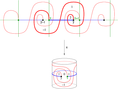
Figure 6: An $(\alpha,\beta)$-trace on the annulus satisfying the arc condition.

Proof of Proposition 5.1.

The proof has five steps.

Step 1. Let ${\widetilde{A}},{\widetilde{B}}\subset{\mathbb{C}}$ be as in Lemma 5.3 and let $g\in\Gamma$ such that

$$g{\widetilde{x}}\in{\widetilde{A}}\setminus{\widetilde{B}},\qquad g{\widetilde{y}}\notin{\widetilde{A}}\cup{\widetilde{B}}.$$

(An example is depicted in Figure 7.) Then (21) holds.

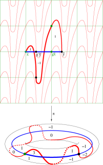
Figure 7: An $(\alpha,\beta)$-trace on the torus not satisfying the arc condition.

The proof is a refinement of the winding number comparison argument in Lemma 5.4. Since $g{\widetilde{x}}\notin{\widetilde{B}}$ we have $g\neq{\rm id}$ and, since ${\widetilde{x}},g{\widetilde{x}}\in{\widetilde{A}}\subset{\widetilde{\alpha}}$, it follows that $\alpha$ is a noncontractible embedded circle. Hence we may choose the universal covering $\pi:{\mathbb{C}}\to\Sigma$ and the lifts ${\widetilde{\alpha}}$, ${\widetilde{\beta}}$, ${\widetilde{\Lambda}}$ such that $\pi({\mathbb{R}})=\alpha$, the map ${\widetilde{z}}\mapsto{\widetilde{z}}+1$ is a deck transformation, the projection $\pi$ maps the interval $[0,1)$ bijectively onto $\alpha$, and

$${\widetilde{\alpha}}={\mathbb{R}},\qquad{\widetilde{x}}=0\in{\widetilde{\alpha}}\cap{\widetilde{\beta}},\qquad{\widetilde{y}}>0.$$

By hypothesis and Lemma 5.3 there is an integer $k$ such that

$$0<k<{\widetilde{y}},\qquad g{\widetilde{x}}=k,\qquad g^{-1}{\widetilde{y}}={\widetilde{y}}-k.$$

Thus $g$ is the deck transformation ${\widetilde{z}}\mapsto{\widetilde{z}}+k$.

Since $g{\widetilde{x}}\notin{\widetilde{B}}$ and $g{\widetilde{y}}\notin{\widetilde{B}}$ it follows from Lemma 5.3 that $g^{-1}{\widetilde{y}}\notin{\widetilde{B}}$ and $g^{-1}{\widetilde{x}}\notin{\widetilde{B}}$ and hence, again by Lemma 5.3, we have

$${\widetilde{B}}\cap g{\widetilde{B}}={\widetilde{B}}\cap g^{-1}{\widetilde{B}}=\emptyset.$$

With $\gamma_{\widetilde{\alpha}}$ and $\gamma_{\widetilde{\beta}}$ chosen as in Lemma 5.3, this implies

$$\gamma_{\widetilde{\beta}}\cdot(\gamma_{\widetilde{\beta}}-k)=(\gamma_{\widetilde{\beta}}+k)\cdot\gamma_{\widetilde{\beta}}=0.$$ (26)

Since $k,-k,{\widetilde{y}}+k,{\widetilde{y}}-k\notin{\widetilde{B}}$, there exists a constant ${\varepsilon}>0$ such that

$$-{\varepsilon}\leq t\leq{\varepsilon}\qquad\implies\qquad k+{\mathbf{i}}t,\;\;-k+{\mathbf{i}}t,\;\;{\widetilde{y}}-k+{\mathbf{i}}t,\;\;{\widetilde{y}}+k+{\mathbf{i}}t\notin{\widetilde{B}}.$$

The paths $g\gamma_{\widetilde{\alpha}}\pm{\mathbf{i}}{\varepsilon}$ and $g\gamma_{\widetilde{\beta}}\pm{\mathbf{i}}{\varepsilon}$ both connect the point $g{\widetilde{x}}\pm{\mathbf{i}}{\varepsilon}$ to $g{\widetilde{y}}\pm{\mathbf{i}}{\varepsilon}$. Likewise, the paths $g^{-1}\gamma_{\widetilde{\alpha}}\pm{\mathbf{i}}{\varepsilon}$ and $g^{-1}\gamma_{\widetilde{\beta}}\pm{\mathbf{i}}{\varepsilon}$ both connect the point $g^{-1}{\widetilde{x}}\pm{\mathbf{i}}{\varepsilon}$ to $g^{-1}{\widetilde{y}}\pm{\mathbf{i}}{\varepsilon}$. Hence

$$\widetilde{\rm w}(g{\widetilde{y}}\pm{\mathbf{i}}{\varepsilon})-\widetilde{\rm w}(g{\widetilde{x}}\pm{\mathbf{i}}{\varepsilon}) = (\gamma_{\widetilde{\alpha}}-\gamma_{\widetilde{\beta}})\cdot(g\gamma_{\widetilde{\alpha}}\pm{\mathbf{i}}{\varepsilon})$$

$$= (\gamma_{\widetilde{\alpha}}-\gamma_{\widetilde{\beta}})\cdot(\gamma_{\widetilde{\alpha}}+k\pm{\mathbf{i}}{\varepsilon})$$

$$= (\gamma_{\widetilde{\alpha}}+k\pm{\mathbf{i}}{\varepsilon})\cdot\gamma_{\widetilde{\beta}}$$

$$= \gamma_{\widetilde{\alpha}}\cdot(\gamma_{\widetilde{\beta}}-k\mp{\mathbf{i}}{\varepsilon})$$

$$= (\gamma_{\widetilde{\alpha}}-\gamma_{\widetilde{\beta}})\cdot(\gamma_{\widetilde{\beta}}-k\mp{\mathbf{i}}{\varepsilon})$$

$$= (\gamma_{\widetilde{\alpha}}-\gamma_{\widetilde{\beta}})\cdot(g^{-1}\gamma_{\widetilde{\beta}}\mp{\mathbf{i}}{\varepsilon})$$

$$= \widetilde{\rm w}(g^{-1}{\widetilde{y}}\mp{\mathbf{i}}{\varepsilon})-\widetilde{\rm w}(g^{-1}{\widetilde{x}}\mp{\mathbf{i}}{\varepsilon}).$$

Here the last but one equation follows from (26). Thus we have proved

$$\begin{split}\widetilde{\rm w}(g{\widetilde{x}}+{\mathbf{i}}{\varepsilon})+\widetilde{\rm w}(g^{-1}{\widetilde{y}}-{\mathbf{i}}{\varepsilon})&=\widetilde{\rm w}(g^{-1}{\widetilde{x}}-{\mathbf{i}}{\varepsilon})+\widetilde{\rm w}(g{\widetilde{y}}+{\mathbf{i}}{\varepsilon}),\\ \widetilde{\rm w}(g{\widetilde{x}}-{\mathbf{i}}{\varepsilon})+\widetilde{\rm w}(g^{-1}{\widetilde{y}}+{\mathbf{i}}{\varepsilon})&=\widetilde{\rm w}(g^{-1}{\widetilde{x}}+{\mathbf{i}}{\varepsilon})+\widetilde{\rm w}(g{\widetilde{y}}-{\mathbf{i}}{\varepsilon}).\end{split}$$ (27)

Since

$$\begin{split}m_{g{\widetilde{x}}}({\widetilde{\Lambda}})&=2\widetilde{\rm w}(g{\widetilde{x}}+{\mathbf{i}}{\varepsilon})+2\widetilde{\rm w}(g{\widetilde{x}}-{\mathbf{i}}{\varepsilon}),\\ m_{g{\widetilde{y}}}({\widetilde{\Lambda}})&=2\widetilde{\rm w}(g{\widetilde{y}}+{\mathbf{i}}{\varepsilon})+2\widetilde{\rm w}(g{\widetilde{y}}-{\mathbf{i}}{\varepsilon}),\\ m_{g^{-1}{\widetilde{x}}}({\widetilde{\Lambda}})&=2\widetilde{\rm w}(g^{-1}{\widetilde{x}}+{\mathbf{i}}{\varepsilon})+2\widetilde{\rm w}(g^{-1}{\widetilde{x}}-{\mathbf{i}}{\varepsilon}),\\ m_{g^{-1}{\widetilde{y}}}({\widetilde{\Lambda}})&=2\widetilde{\rm w}(g^{-1}{\widetilde{y}}+{\mathbf{i}}{\varepsilon})+2\widetilde{\rm w}(g^{-1}{\widetilde{y}}-{\mathbf{i}}{\varepsilon}),\end{split}$$

Step 1 follows by taking the sum of the two equations in (27).

Step 2. Let ${\widetilde{A}},{\widetilde{B}}\subset{\mathbb{C}}$ be as in Lemma 5.3 and let $g\in\Gamma$. Suppose that either $g{\widetilde{x}},g{\widetilde{y}}\notin{\widetilde{A}}$ or $g{\widetilde{x}},g{\widetilde{y}}\notin{\widetilde{B}}$. Then (21) holds.

If $g{\widetilde{x}},g{\widetilde{y}}\notin{\widetilde{A}}\cup{\widetilde{B}}$ the assertion follows from Lemma 5.4. If $g{\widetilde{x}}\in{\widetilde{A}}\setminus{\widetilde{B}}$ and $g{\widetilde{y}}\notin{\widetilde{A}}\cup{\widetilde{B}}$ the assertion follows from Step 1. If $g{\widetilde{x}}\notin{\widetilde{A}}\cup{\widetilde{B}}$ and $g{\widetilde{y}}\in{\widetilde{A}}\setminus{\widetilde{B}}$ the assertion follows from Step 1 by interchanging ${\widetilde{x}}$ and ${\widetilde{y}}$. Namely, (21) holds for ${\widetilde{\Lambda}}$ if and only if it holds for the $({\widetilde{\alpha}},{\widetilde{\beta}})$-trace $-{\widetilde{\Lambda}}:=({\widetilde{y}},{\widetilde{x}},-\widetilde{\rm w}).$ This covers the case $g{\widetilde{x}},g{\widetilde{y}}\notin{\widetilde{B}}$. If $g{\widetilde{x}},g{\widetilde{y}}\notin{\widetilde{A}}$ the assertion follows by interchanging ${\widetilde{A}}$ and ${\widetilde{B}}$. Namely, (21) holds for ${\widetilde{\Lambda}}$ if and only if it holds for the $({\widetilde{\beta}},{\widetilde{\alpha}})$-trace ${\widetilde{\Lambda}}^{*}:=({\widetilde{x}},{\widetilde{y}},-\widetilde{\rm w}).$ This proves Step 2.

Step 3. Let ${\widetilde{A}},{\widetilde{B}}\subset{\mathbb{C}}$ be as in Lemma 5.3 and let $g\in\Gamma$ such that

$$g{\widetilde{x}}\in{\widetilde{A}}\setminus{\widetilde{B}},\qquad g{\widetilde{y}}\in{\widetilde{B}}\setminus{\widetilde{A}}.$$

(An example is depicted in Figure 8.) Then the cancellation formula (20) holds for $g$ and $g^{-1}$.

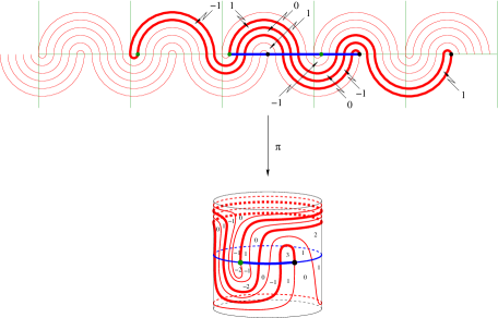
Figure 8: An $(\alpha,\beta)$-trace on the annulus with $g{\widetilde{x}}\in{\widetilde{A}}$ and $g{\widetilde{y}}\in{\widetilde{B}}$.

Since $g{\widetilde{x}}\notin{\widetilde{B}}$ (and $g{\widetilde{y}}\notin{\widetilde{A}}$) we have $g\neq{\rm id}$ and, since ${\widetilde{x}},g{\widetilde{x}}\in{\widetilde{A}}\subset{\widetilde{\alpha}}$ and ${\widetilde{y}},g{\widetilde{y}}\in{\widetilde{B}}\subset{\widetilde{\beta}}$, it follows that $g{\widetilde{\alpha}}={\widetilde{\alpha}}$ and $g{\widetilde{\beta}}={\widetilde{\beta}}$. Hence $\alpha$ and $\beta$ are noncontractible embedded circles and some iterate of $\alpha$ is homotopic to some iterate of $\beta$. So $\alpha$ is homotopic to $\beta$ (with some orientation), by Lemma A.4.

Choose the universal covering $\pi:{\mathbb{C}}\to\Sigma$ and the lifts ${{\widetilde{\alpha}},{\widetilde{\beta}},{\widetilde{\Lambda}}}$ such that $\pi({\mathbb{R}})=\alpha$, the map ${\widetilde{z}}\mapsto{\widetilde{z}}+1$ is a deck transformation, $\pi$ maps the interval $[0,1)$ bijectively onto $\alpha$, and

$${\widetilde{\alpha}}={\mathbb{R}},\qquad{\widetilde{x}}=0\in{\widetilde{\alpha}}\cap{\widetilde{\beta}},\qquad{\widetilde{y}}>0.$$

Thus ${\widetilde{A}}=[0,{\widetilde{y}}]$ is the arc in ${\widetilde{\alpha}}$ from $0$ to ${\widetilde{y}}$ and ${\widetilde{B}}$ is the arc in ${\widetilde{\beta}}$ from $0$ to ${\widetilde{y}}$. Moreover, since $\alpha$ is homotopic to $\beta$, we have

$${\widetilde{\beta}}={\widetilde{\beta}}+1$$

and the arc in ${\widetilde{\beta}}$ from $0$ to $1$ is a fundamental domain for $\beta$. Since $g{\widetilde{\alpha}}={\widetilde{\alpha}}$, the deck transformation $g$ is given by ${\widetilde{z}}\mapsto{\widetilde{z}}+\ell$ for some integer $\ell$. Since $g{\widetilde{x}}\in{\widetilde{A}}\setminus{\widetilde{B}}$ and $g{\widetilde{y}}\in{\widetilde{B}}$, we have $g^{-1}{\widetilde{y}}\notin{\widetilde{B}}$ and $g^{-1}{\widetilde{x}}\in{\widetilde{B}}$ by Lemma 5.3. Hence

$$0<\ell<{\widetilde{y}},\qquad\ell\notin{\widetilde{B}},\qquad{\widetilde{y}}+\ell\in{\widetilde{B}},\qquad{\widetilde{y}}-\ell\notin{\widetilde{B}},\qquad-\ell\in{\widetilde{B}}.$$

This shows that, walking along ${\widetilde{\beta}}$ from $0$ to ${\widetilde{y}}$ (traversing ${\widetilde{B}}$) one encounters some negative integer and therefore no positive integers. Hence

$${\widetilde{A}}\cap{\mathbb{Z}}=\left\{0,1,2,\cdots,k_{\widetilde{A}}\right\},\qquad{\widetilde{B}}\cap{\mathbb{Z}}=\left\{0,-1,-2,\cdots,-k_{\widetilde{B}}\right\},$$

where $k_{\widetilde{A}}$ is the number of fundamental domains of ${\widetilde{\alpha}}$ contained in ${\widetilde{A}}$ and $k_{\widetilde{B}}$ is the number of fundamental domains of ${\widetilde{\beta}}$ contained in ${\widetilde{B}}$ (see Figure 8). For $0\leq k\leq k_{\widetilde{A}}$ let ${\widetilde{A}}_{k}\subset{\widetilde{\alpha}}$ and ${\widetilde{B}}_{k}\subset{\widetilde{\beta}}$ be the arcs from $0$ to ${\widetilde{y}}-k$. Thus ${\widetilde{A}}_{k}$ is obtained from ${\widetilde{A}}$ by removing $k$ fundamental domains at the end, while ${\widetilde{B}}_{k}$ is obtained from ${\widetilde{B}}$ by attaching $k$ fundamental domains at the end. Consider the $({\widetilde{\alpha}},{\widetilde{\beta}})$-trace

$${\widetilde{\Lambda}}_{k}:=(0,{\widetilde{y}}-k,\widetilde{\rm w}_{k}),\qquad{\partial}{\widetilde{\Lambda}}_{k}:=(0,{\widetilde{y}}-k,{\widetilde{A}}_{k},{\widetilde{B}}_{k}),$$

where $\widetilde{\rm w}_{k}:{\mathbb{C}}\setminus({\widetilde{A}}_{k}\cup{\widetilde{B}}_{k})\to{\mathbb{Z}}$ is the winding number of ${\widetilde{A}}_{k}-{\widetilde{B}}_{k}$. Then

$${\widetilde{B}}_{k}\cap{\mathbb{Z}}=\left\{0,-1,-2,\cdots,-k_{\widetilde{B}}-k\right\}$$

and ${\widetilde{\Lambda}}_{0}={\widetilde{\Lambda}}$. We prove that, for each $k$, the $({\widetilde{\alpha}},{\widetilde{\beta}})$-trace ${\widetilde{\Lambda}}_{k}$ satisfies

$$m_{j}({\widetilde{\Lambda}}_{k})+m_{{\widetilde{y}}-k-j}({\widetilde{\Lambda}}_{k})=0\qquad\forall\,j\in{\mathbb{Z}}\setminus\{0\}.$$ (28)

If ${\widetilde{y}}$ is an integer, then (28) follows from Lemma 5.5. Hence we may assume that ${\widetilde{y}}$ is not an integer.

We prove equation (28) by reverse induction on $k$. First let $k=k_{\widetilde{A}}$. Then we have $j,{\widetilde{y}}-k+j\notin{\widetilde{A}}_{k}$ for every $j\in{\mathbb{N}}$. Hence it follows from Step 2 that

$$m_{j}({\widetilde{\Lambda}}_{k})+m_{{\widetilde{y}}-k-j}({\widetilde{\Lambda}}_{k})=m_{-j}({\widetilde{\Lambda}}_{k})+m_{{\widetilde{y}}-k+j}({\widetilde{\Lambda}})\qquad\forall\,j\in{\mathbb{N}}.$$ (29)

Thus we can apply Lemma 5.2 to the projection of ${\widetilde{\Lambda}}_{k}$ to the quotient ${\mathbb{C}}/{\mathbb{Z}}$. Hence ${\widetilde{\Lambda}}_{k}$ satisfies (28).

Now fix an integer $k\in\{0,1,\dots,k_{\widetilde{A}}-1\}$ and suppose, by induction, that ${\widetilde{\Lambda}}_{k+1}$ satisfies (28). Denote by ${\widetilde{A}}^{\prime}\subset{\widetilde{\alpha}}$ and ${\widetilde{B}}^{\prime}\subset{\widetilde{\beta}}$ the arcs from ${\widetilde{y}}-k-1$ to $1$, and by ${\widetilde{A}}^{\prime\prime}\subset{\widetilde{\alpha}}$ and ${\widetilde{B}}^{\prime\prime}\subset{\widetilde{\beta}}$ the arcs from $1$ to ${\widetilde{y}}-k$. Then ${\widetilde{\Lambda}}_{k}$ is the catenation of the $({\widetilde{\alpha}},{\widetilde{\beta}})$-traces

$$\begin{split}{\widetilde{\Lambda}}_{k+1}:=(0,{\widetilde{y}}-k-1,\widetilde{\rm w}_{k+1}),\quad&{\partial}{\widetilde{\Lambda}}_{k+1}=(0,{\widetilde{y}}-k-1,{\widetilde{A}}_{k+1},{\widetilde{B}}_{k+1}),\\ {\widetilde{\Lambda}}^{\prime}:=({\widetilde{y}}-k-1,1,\widetilde{\rm w}^{\prime}),\quad&{\partial}{\widetilde{\Lambda}}^{\prime}=({\widetilde{y}}-k-1,1,{\widetilde{A}}^{\prime},{\widetilde{B}}^{\prime}),\\ {\widetilde{\Lambda}}^{\prime\prime}:=(1,{\widetilde{y}}-k,\widetilde{\rm w}^{\prime\prime}),\quad&{\partial}{\widetilde{\Lambda}}^{\prime\prime}=(1,{\widetilde{y}}-k,{\widetilde{A}}^{\prime\prime},{\widetilde{B}}^{\prime\prime}).\end{split}$$

Here $\widetilde{\rm w}^{\prime}({\widetilde{z}})$ is the winding number of the loop ${\widetilde{A}}^{\prime}-{\widetilde{B}}^{\prime}$ about ${\widetilde{z}}\in{\mathbb{C}}\setminus({\widetilde{A}}^{\prime}\cup{\widetilde{B}}^{\prime})$ and simiarly for $\widetilde{\rm w}^{\prime\prime}$. Note that ${\widetilde{\Lambda}}^{\prime\prime}$ is the shift of ${\widetilde{\Lambda}}_{k+1}$ by $1$. The catenation of ${\widetilde{\Lambda}}_{k+1}$ and ${\widetilde{\Lambda}}^{\prime}$ is the $({\widetilde{\alpha}},{\widetilde{\beta}})$-trace from $0$ to $1$. Hence it has Viterbo–Maslov index zero, by Lemma 5.5, and satisfies

$$m_{j}({\widetilde{\Lambda}}_{k+1})+m_{j}({\widetilde{\Lambda}}^{\prime})=0\qquad\forall j\in{\mathbb{Z}}\setminus\{0,1\}.$$ (30)

Since the catenation of ${\widetilde{\Lambda}}^{\prime}$ and ${\widetilde{\Lambda}}^{\prime\prime}$ is the $({\widetilde{\alpha}},{\widetilde{\beta}})$-trace from ${\widetilde{y}}-k-1$ to ${\widetilde{y}}-k$, it also has Viterbo–Maslov index zero and satisfies

$$m_{{\widetilde{y}}-k-j}({\widetilde{\Lambda}}^{\prime})+m_{{\widetilde{y}}-k-j}({\widetilde{\Lambda}}^{\prime\prime})=0\qquad\forall j\in{\mathbb{Z}}\setminus\{0,1\}.$$ (31)

Moreover, by the induction hypothesis, we have

$$m_{j}({\widetilde{\Lambda}}_{k+1})+m_{{\widetilde{y}}-k-1-j}({\widetilde{\Lambda}}_{k+1})=0\qquad\forall j\in{\mathbb{Z}}\setminus\{0\}.$$ (32)

Combining the equations (30), (31), (32) we find that, for $j\in{\mathbb{Z}}\setminus\{0,1\}$,

$$m_{j}({\widetilde{\Lambda}}_{k})+m_{{\widetilde{y}}-k-j}({\widetilde{\Lambda}}_{k}) = m_{j}({\widetilde{\Lambda}}_{k+1})+m_{j}({\widetilde{\Lambda}}^{\prime})+m_{j}({\widetilde{\Lambda}}^{\prime\prime})$$

$$+\,m_{{\widetilde{y}}-k-j}({\widetilde{\Lambda}}_{k+1})+m_{{\widetilde{y}}-k-j}({\widetilde{\Lambda}}^{\prime})+m_{{\widetilde{y}}-k-j}({\widetilde{\Lambda}}^{\prime\prime})$$

$$= m_{j}({\widetilde{\Lambda}}_{k+1})+m_{j}({\widetilde{\Lambda}}^{\prime})$$

$$+\,m_{{\widetilde{y}}-k-j}({\widetilde{\Lambda}}^{\prime})+m_{{\widetilde{y}}-k-j}({\widetilde{\Lambda}}^{\prime\prime})$$

$$+\,m_{j-1}({\widetilde{\Lambda}}_{k+1})+m_{{\widetilde{y}}-k-j}({\widetilde{\Lambda}}_{k+1})$$

$$= 0.$$

For $j=1$ we obtain

$$m_{1}({\widetilde{\Lambda}}_{k})+m_{{\widetilde{y}}-k-1}({\widetilde{\Lambda}}_{k}) = m_{1}({\widetilde{\Lambda}}_{k+1})+m_{1}({\widetilde{\Lambda}}^{\prime})+m_{1}({\widetilde{\Lambda}}^{\prime\prime})$$

$$+\,m_{{\widetilde{y}}-k-1}({\widetilde{\Lambda}}_{k+1})+m_{{\widetilde{y}}-k-1}({\widetilde{\Lambda}}^{\prime})+m_{{\widetilde{y}}-k-1}({\widetilde{\Lambda}}^{\prime\prime})$$

$$= m_{1}({\widetilde{\Lambda}}_{k+1})+m_{{\widetilde{y}}-k-2}({\widetilde{\Lambda}}_{k+1})$$

$$+\,m_{0}({\widetilde{\Lambda}}_{k+1})+m_{{\widetilde{y}}-k-1}({\widetilde{\Lambda}}_{k+1})$$

$$+\,m_{{\widetilde{y}}-k-1}({\widetilde{\Lambda}}^{\prime})+m_{1}({\widetilde{\Lambda}}^{\prime})$$

$$= 2\mu({\widetilde{\Lambda}}_{k+1})+2\mu({\widetilde{\Lambda}}^{\prime})$$

$$= 0.$$

Here the last but one equation follows from equation (32) and Proposition 4.1, and the last equation follows from Lemma 5.5. Hence ${\widetilde{\Lambda}}_{k}$ satisfies (28). This completes the induction argument for the proof of Step 3.

Step 4. Let ${\widetilde{A}},{\widetilde{B}}\subset{\mathbb{C}}$ be as in Lemma 5.3 and let $g\in\Gamma$ such that

$$g{\widetilde{x}}\in{\widetilde{A}}\cap{\widetilde{B}},\qquad g{\widetilde{y}}\notin{\widetilde{A}}\cup{\widetilde{B}}.$$

Then the cancellation formula (20) holds for $g$ and $g^{-1}$.

The proof is by induction and catenation based on Step 2 and Lemma 5.5. Since $g{\widetilde{y}}\notin{\widetilde{A}}\cup{\widetilde{B}}$ we have $g\neq{\rm id}$. Since $g{\widetilde{x}}\in{\widetilde{A}}\cap{\widetilde{B}}$ we have ${\widetilde{\alpha}}=g{\widetilde{\alpha}}$ and ${\widetilde{\beta}}=g{\widetilde{\beta}}$. Hence $\alpha$ and $\beta$ are noncontractible embedded circles, and they are homotopic (with some orientation) by Lemma A.4. Thus we may choose $\pi:{\mathbb{C}}\to\Sigma$, ${\widetilde{\alpha}}$, ${\widetilde{\beta}}$, ${\widetilde{\Lambda}}$ as in Step 3. By hypothesis there is an integer $k\in{\widetilde{A}}\cap{\widetilde{B}}$. Hence ${\widetilde{A}}$ and ${\widetilde{B}}$ do not contain any negative integers. Choose $k_{\widetilde{A}},k_{\widetilde{B}}\in{\mathbb{N}}$ such that

$${\widetilde{A}}\cap{\mathbb{Z}}=\left\{0,1,\dots,k_{\widetilde{A}}\right\},\qquad{\widetilde{B}}\cap{\mathbb{Z}}=\left\{0,1,\dots,k_{\widetilde{B}}\right\}.$$

Assume without loss of generality that

$$k_{\widetilde{A}}\leq k_{\widetilde{B}}.$$

For $0\leq k\leq k_{\widetilde{A}}$ denote by ${\widetilde{A}}_{k}\subset{\widetilde{A}}$ and ${\widetilde{B}}_{k}\subset{\widetilde{B}}$ the arcs from $0$ to ${\widetilde{y}}-k$ and consider the $({\widetilde{\alpha}},{\widetilde{\beta}})$-trace

$${\widetilde{\Lambda}}_{k}:=(0,{\widetilde{y}}-k,\widetilde{\rm w}_{k}),\qquad{\partial}{\widetilde{\Lambda}}_{k}:=(0,{\widetilde{y}}-k,{\widetilde{A}}_{k},{\widetilde{B}}_{k}).$$

In this case

$${\widetilde{B}}_{k}\cap{\mathbb{Z}}=\{0,1,\dots,k_{\widetilde{B}}-k\}.$$

As in Step 3, it follows by reverse induction on $k$ that ${\widetilde{\Lambda}}_{k}$ satisfies (28) for every $k$. We assume again that ${\widetilde{y}}$ is not an integer. (Otherwise (28) follows from Lemma 5.5). If $k=k_{\widetilde{A}}$ then $j,{\widetilde{y}}-k+j\notin{\widetilde{A}}_{k}$ for every $j\in{\mathbb{N}}$, hence it follows from Step 2 that ${\widetilde{\Lambda}}_{k}$ satisfies (29), and hence it follows from Lemma 5.2 for the projection of ${\widetilde{\Lambda}}_{k}$ to the annulus ${\mathbb{C}}/{\mathbb{Z}}$ that ${\widetilde{\Lambda}}_{k}$ also satisfies (28). The induction step is verbatim the same as in Step 3 and will be omitted. This proves Step 4.

Step 5. We prove Proposition 5.1.

If both points $g{\widetilde{x}},g{\widetilde{y}}$ are contained in ${\widetilde{A}}$ (or in ${\widetilde{B}}$) then $g={\rm id}$ by Lemma 5.3, and in this case equation (21) is a tautology. If both points $g{\widetilde{x}},g{\widetilde{y}}$ are not contained in ${\widetilde{A}}\cup{\widetilde{B}}$, equation (21) has been established in Lemma 5.4. Moreover, we can interchange ${\widetilde{x}}$ and ${\widetilde{y}}$ or ${\widetilde{A}}$ and ${\widetilde{B}}$ as in the proof of Step 2. Thus Steps 1 and 4 cover the case where precisely one of the points $g{\widetilde{x}},g{\widetilde{y}}$ is contained in ${\widetilde{A}}\cup{\widetilde{B}}$ while Step 3 covers the case where $g\neq{\rm id}$ and both points $g{\widetilde{x}},g{\widetilde{y}}$ are contained in ${\widetilde{A}}\cup{\widetilde{B}}$. This shows that equation (21) holds for every $g\in\Gamma\setminus\{{\rm id}\}$. Hence, by Lemma 5.2, the cancellation formula (20) holds for every $g\in\Gamma\setminus\{{\rm id}\}$. This proves Proposition 5.1. ∎

Proof of Theorem 3.4 in the Non Simply Connected Case.

Choose a universal covering $\pi:{\mathbb{C}}\to\Sigma$ and let $\Gamma$, ${\widetilde{\alpha}}$, ${\widetilde{\beta}}$, and ${\widetilde{\Lambda}}=({\widetilde{x}},{\widetilde{y}},\widetilde{\rm w})$ be as in Proposition 5.1. Then

$$m_{x}(\Lambda)+m_{y}(\Lambda)-m_{\widetilde{x}}({\widetilde{\Lambda}})-m_{\widetilde{y}}({\widetilde{\Lambda}})=\sum_{g\neq{\rm id}}\left(m_{g{\widetilde{x}}}({\widetilde{\Lambda}})+m_{g^{-1}{\widetilde{y}}}({\widetilde{\Lambda}})\right)=0.$$

Here the last equation follows from the cancellation formula in Proposition 5.1. Hence, by Proposition 4.1, we have

$$\mu(\Lambda)=\mu({\widetilde{\Lambda}})=\frac{m_{\widetilde{x}}({\widetilde{\Lambda}})+m_{\widetilde{y}}({\widetilde{\Lambda}})}{2}=\frac{m_{x}(\Lambda)+m_{y}(\Lambda)}{2}.$$

This proves the trace formula in the case where $\Sigma$ is not simply connected. ∎

II. Combinatorial Lunes

6 Lunes and Traces

We denote the universal covering of $\Sigma$ by

$$\pi:{\widetilde{\Sigma}}\to\Sigma$$

and, when $\Sigma$ is not diffeomorphic to the $2$-sphere, we assume ${\widetilde{\Sigma}}={\mathbb{C}}$.

Definition 6.1 (Smooth Lunes).

Assume (H). A smooth $(\alpha,\beta)$-lune is an orientation preserving immersion $u:{\mathbb{D}}\to\Sigma$ such that

$$u({\mathbb{D}}\cap{\mathbb{R}})\subset\alpha,\qquad u({\mathbb{D}}\cap S^{1})\subset\beta,$$

Three examples of smooth lunes are depicted in Figure 9. Two lunes are said to be equivalent iff there is an orientation preserving diffeomorphism ${\varphi}:{\mathbb{D}}\to{\mathbb{D}}$ such that

$${\varphi}(-1)=-1,\qquad{\varphi}(1)=1,\qquad u^{\prime}=u\circ{\varphi}.$$

The equivalence class of $u$ is denoted by $[u]$. That $u$ is an immersion means that $u$ is smooth and $du$ is injective in all of ${\mathbb{D}}$, even at the corners $\pm 1$. The set $u({\mathbb{D}}\cap{\mathbb{R}})$ is called the bottom boundary of the lune, and the set $u({\mathbb{D}}\cap S^{1})$ is called the top boundary. The points

$$x=u(-1),\qquad y=u(1)$$

are called respectively the left and right endpoints of the lune. The locally constant function

$$\Sigma\setminus u({\partial}{\mathbb{D}})\to{\mathbb{N}}:z\mapsto\#u^{-1}(z)$$

is called the counting function of the lune. (This function is locally constant because a proper local homeomorphism is a covering projection.) A smooth lune is said to be embedded iff the map $u$ is injective. These notions depend only on the equivalence class $[u]$ of the smooth lune $u$.

Our objective is to characterize smooth lunes in terms of their boundary behavior, i.e. to say when a pair of immersions ${u_{\alpha}:({\mathbb{D}}\cap{\mathbb{R}},-1,1)\to(\alpha,x,y)}$ and ${u_{\beta}:({\mathbb{D}}\cap S^{1},-1,1)\to(\beta,x,y)}$ extends to a smooth $(\alpha,\beta)$-lune $u$. Recall the following definitions and theorems from Part I.

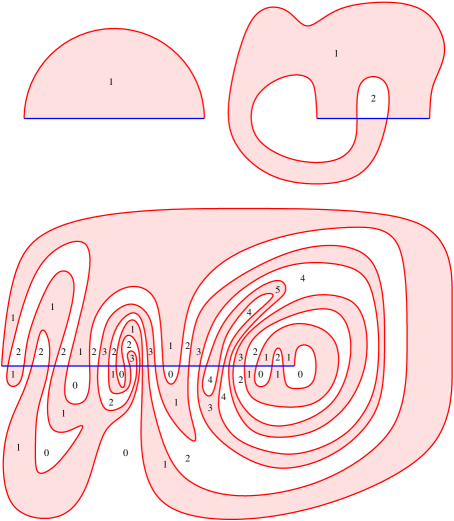
Figure 9: Three lunes.

Definition 6.2 (Traces).

Assume (H). An $(\alpha,\beta)$-trace is a triple

$$\Lambda=(x,y,{\rm w})$$

such that $x,y\in\alpha\cap\beta$ and ${\rm w}:\Sigma\setminus(\alpha\cup\beta)\to{\mathbb{Z}}$ is a locally constant function such that there exists a smooth map $u:{\mathbb{D}}\to\Sigma$ satisfying

$$u({\mathbb{D}}\cap{\mathbb{R}})\subset\alpha,\qquad u({\mathbb{D}}\cap S^{1})\subset\beta,$$ (33)

$$u(-1)=x,\qquad u(1)=y,$$ (34)

$${\rm w}(z)=\deg(u,z),\qquad z\in\Sigma\setminus(\alpha\cup\beta).$$ (35)

The $(\alpha,\beta)$-trace associated to a smooth map $u:{\mathbb{D}}\to\Sigma$ satisfying (33) is denoted by $\Lambda_{u}$.

The boundary of an $(\alpha,\beta)$-trace $\Lambda=(x,y,{\rm w})$ is the triple

$${\partial}\Lambda:=(x,y,{\partial}{\rm w}).$$

Here

$${\partial}{\rm w}:(\alpha\setminus\beta)\cup(\beta\setminus\alpha)\to{\mathbb{Z}}$$

is the locally constant function that assigns to $z\in\alpha\setminus\beta$ the value of ${\rm w}$ slightly to the left of $\alpha$ minus the value of ${\rm w}$ slightly to the right of $\alpha$ near $z$, and to $z\in\beta\setminus\alpha$ the value of ${\rm w}$ slightly to the right of $\beta$ minus the value of ${\rm w}$ slightly to the left of $\beta$ near $z$.

In Lemma 2.3 above it was shown that, if $\Lambda=(x,y,{\rm w})$ is the $(\alpha,\beta)$-trace of a smooth map $u:{\mathbb{D}}\to\Sigma$ that satisfies (33), then ${\partial}\Lambda_{u}=(x,y,\nu)$, where the function $\nu:={\partial}{\rm w}:(\alpha\setminus\beta)\cup(\beta\setminus\alpha)\to{\mathbb{Z}}$ is given by

$$\nu(z)=\left\{\begin{array}[]{rl}\deg(u\big{|}_{{\partial}{\mathbb{D}}\cap{\mathbb{R}}\;\,}:{\partial}{\mathbb{D}}\cap{\mathbb{R}}\;\to\alpha,z),&\mbox{for }z\in\alpha\setminus\beta,\\ -\deg(u\big{|}_{{\partial}{\mathbb{D}}\cap S^{1}}:{\partial}{\mathbb{D}}\cap S^{1}\to\beta,z),&\mbox{for }z\in\beta\setminus\alpha.\end{array}\right.$$ (36)

Here we orient the one-manifolds ${\mathbb{D}}\cap{\mathbb{R}}$ and ${\mathbb{D}}\cap S^{1}$ from $-1$ to $+1$. Moreover, in Theorem 2.4 above it was shown that the homotopy class of a smooth map $u:{\mathbb{D}}\to\Sigma$ satisfying the boundary condition (33) is uniquely determined by its trace $\Lambda_{u}=(x,y,{\rm w})$. If $\Sigma$ is not diffeomorphic to the $2$-sphere then its universal cover is diffeomorphic to the $2$-plane. In this situation it was also shown in Theorem 2.4 that the homotopy class of $u$ and the degree function ${\rm w}$ are uniquely determined by the triple ${\partial}\Lambda_{u}=(x,y,\nu)$.

Remark 6.3 (The Viterbo–Maslov index).

Let $\Lambda=(x,y,{\rm w})$ be an $(\alpha,\beta)$-trace and denote by $\mu(\Lambda)$ its Viterbo–Maslov index as defined in 3.1 above (see also [39]). For $z\in\alpha\cap\beta$ let $m_{z}(\Lambda)$ be the sum of the four values of the function ${\rm w}$ encountered when walking along a small circle surrounding $z$. In Theorem 3.4 it was shown that the Viterbo–Maslov index of $\Lambda$ is given by the trace formula

$$\mu(\Lambda)=\frac{m_{x}(\Lambda)+m_{y}(\Lambda)}{2}.$$ (37)

Let $\Lambda^{\prime}=(y,z,{\rm w}^{\prime})$ be another $(\alpha,\beta)$-trace. The catenation of $\Lambda$ and $\Lambda^{\prime}$ is defined by

$$\Lambda\#\Lambda^{\prime}:=(x,z,{\rm w}+{\rm w}^{\prime}).$$

It is again an $(\alpha,\beta)$-trace and has Viterbo–Maslov index

$$\mu(\Lambda\#\Lambda^{\prime})=\mu(\Lambda)+\mu(\Lambda^{\prime}).$$ (38)

For a proof see [39, 30].

Definition 6.4 (Arc Condition).

Let $\Lambda=(x,y,{\rm w})$ be an $(\alpha,\beta)$-trace and

$$\nu_{\alpha}:={\partial}{\rm w}|_{\alpha\setminus\beta},\qquad\nu_{\beta}:=-{\partial}{\rm w}|_{\beta\setminus\alpha}.$$

$\Lambda$ is said to satisfy the arc condition if

$$x\neq y,\qquad\min\left|\nu_{\alpha}\right|=\min\left|\nu_{\beta}\right|=0.$$ (39)

When $\Lambda$ satisfies the arc condition there are arcs $A\subset\alpha$ and $B\subset\beta$ from $x$ to $y$ such that

$$\nu_{\alpha}(z)=\left\{\begin{array}[]{rl}\pm 1,&\mbox{if }z\in A,\\ 0,&\mbox{if }z\in\alpha\setminus\overline{A},\end{array}\right.\;\;\nu_{\beta}(z)=\left\{\begin{array}[]{rl}\pm 1,&\mbox{if }z\in B,\\ 0,&\mbox{if }z\in\beta\setminus\overline{B}.\end{array}\right.$$ (40)

Here the plus sign is chosen iff the orientation of $A$ from $x$ to $y$ agrees with that of $\alpha$, respectively the orientation of $B$ from $x$ to $y$ agrees with that of $\beta$. In this situation the quadruple $(x,y,A,B)$ and the triple $(x,y,{\partial}{\rm w})$ determine one another and we also write

$${\partial}\Lambda=(x,y,A,B)$$

for the boundary of $\Lambda$. When $u:{\mathbb{D}}\to\Sigma$ is a smooth map satisfying (33) and $\Lambda_{u}=(x,y,{\rm w})$ satisfies the arc condition and ${\partial}\Lambda_{u}=(x,y,A,B)$ then the path $s\mapsto u(-\cos(\pi s),0)$ is homotopic in $\alpha$ to a path traversing $A$ and the path $s\mapsto u(-\cos(\pi s),\sin(\pi s))$ is homotopic in $\beta$ to a path traversing $B$.

Theorem 6.5.

Assume (H). If $u:{\mathbb{D}}\to\Sigma$ is a smooth $(\alpha,\beta)$-lune then its $(\alpha,\beta)$-trace $\Lambda_{u}$ satisfies the arc condition.

Proof.

See Section 7 page 7. ∎

Definition 6.6 (Combinatorial Lunes).

Assume (H). A combinatorial $(\alpha,\beta)$-lune is an $(\alpha,\beta)$-trace $\Lambda=(x,y,{\rm w})$ with boundary ${\partial}\Lambda=:(x,y,A,B)$ that satisfies the arc condition and the following.

(I)

${\rm w}(z)\geq 0$ for every $z\in\Sigma\setminus(\alpha\cup\beta)$.

(II)

The intersection index of $A$ and $B$ at $x$ is $+1$ and at $y$ is $-1$.

(III)

${\rm w}(z)\in\{0,1\}$ for $z$ sufficiently close to $x$ or $y$.

Condition (II) says that the angle from $A$ to $B$ at $x$ is between zero and $\pi$ and the angle from $B$ to $A$ at $y$ is also between zero and $\pi$.

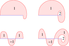
Figure 10: $(\alpha,\beta)$-traces which satisfy the arc condition but are not lunes.

Theorem 6.7 (Existence).

Assume (H) and let $\Lambda=(x,y,{\rm w})$ be an $(\alpha,\beta)$-trace. Consider the following three conditions.

(i) There exists a smooth $(\alpha,\beta)$-lune $u$ such that $\Lambda_{u}=\Lambda$.

(ii) ${\rm w}\geq 0$ and $\mu(\Lambda)=1$.

(iii) $\Lambda$ is a combinatorial $(\alpha,\beta)$-lune.

Then (i)$\implies$(ii)$\iff$(iii). If $\Sigma$ is simply connected then all three conditions are equivalent.

Proof.

See Section 8 page 8. ∎

Theorem 6.8 (Uniqueness).

Assume (H). If two smooth $(\alpha,\beta)$-lunes have the same trace then they are equivalent.

Proof.

See Section 8 page 8. ∎

Corollary 6.9.

Assume (H) and let

$$\Lambda=(x,y,{\rm w})$$

be an $(\alpha,\beta)$-trace. Choose a universal covering $\pi:{\widetilde{\Sigma}}\to\Sigma$, a point

$${\widetilde{x}}\in\pi^{-1}(x),$$

and lifts ${\widetilde{\alpha}}$ and ${\widetilde{\beta}}$ of $\alpha$ and $\beta$ such that

$${\widetilde{x}}\in{\widetilde{\alpha}}\cap{\widetilde{\beta}}.$$

Let

$${\widetilde{\Lambda}}=({\widetilde{x}},{\widetilde{y}},\widetilde{\rm w})$$

be the lift of $\Lambda$ to the universal cover.

(i) If ${\widetilde{\Lambda}}$ is a combinatorial $({\widetilde{\alpha}},{\widetilde{\beta}})$-lune then $\Lambda$ is a combinatorial $(\alpha,\beta)$-lune.

(ii) ${\widetilde{\Lambda}}$ is a combinatorial $({\widetilde{\alpha}},{\widetilde{\beta}})$-lune if and only if there exists a smooth $(\alpha,\beta)$-lune $u$ such that $\Lambda_{u}=\Lambda$.

Proof.

Lifting defines a one-to-one correspondence between smooth $(\alpha,\beta)$-lunes with trace $\Lambda$ and smooth $({\widetilde{\alpha}},{\widetilde{\beta}})$-lunes with trace ${\widetilde{\Lambda}}$. Hence the assertions follow from Theorem 6.7. ∎

Remark 6.10.

Assume (H) and let $\Lambda$ be an $(\alpha,\beta)$-trace. We conjecture that the three conditions in Theorem 6.7 are equivalent, even when $\Sigma$ is not simply connected, i.e.

If $\Lambda$ is a combinatorial $(\alpha,\beta)$-lune

then there exists a smooth $(\alpha,\beta)$-lune $u$ such that $\Lambda=\Lambda_{u}$.

Theorem 6.7 shows that this conjecture is equivalent to the following.

If $\Lambda$ is a combinatorial $(\alpha,\beta)$-lune

then ${\widetilde{\Lambda}}$ is a combinatorial $({\widetilde{\alpha}},{\widetilde{\beta}})$-lune.

The hard part is to prove that ${\widetilde{\Lambda}}$ satisfies (I), i.e. that the winding numbers are nonnegative.

Remark 6.11.

Assume (H). Corollary 6.9 and Theorem 6.8 suggest the following algorithm for finding a smooth $(\alpha,\beta)$-lune.

1. Fix two points $x,y\in\alpha\cap\beta$ with opposite intersection indices, and two oriented embedded arcs $A\subset\alpha$ and $B\subset\beta$ from $x$ to $y$ so that (II) holds.

2. If $A$ is not homotopic to $B$ with fixed endpoints discard this pair. Otherwise $(x,y,A,B)$ is the boundary of an $(\alpha,\beta)$-trace $\Lambda=(x,y,{\rm w})$ satisfying the arc condition and (II) (for a suitable function ${\rm w}$ to be chosen below).

3a. If $\Sigma$ is diffeomorphic to the $2$-sphere let ${\rm w}:\Sigma\setminus(A\cup B)\to{\mathbb{Z}}$ be the winding number of the loop $A-B$ in $\Sigma\setminus\{z_{0}\}$, where $z_{0}\in\alpha\setminus A$ is chosen close to $x$. Check if ${\rm w}$ satisfies (I) and (III). If yes, then $\Lambda=(x,y,{\rm w})$ is a combinatorial $(\alpha,\beta)$-lune and hence, by Theorems 6.7 and 6.8, gives rise to a smooth $(\alpha,\beta)$-lune $u$, unique up to isotopy.

3b. If $\Sigma$ is not diffeomorphic to the $2$-sphere choose lifts ${\widetilde{A}}$ of $A$ and ${\widetilde{B}}$ of $B$ to a universal covering $\pi:{\mathbb{C}}\to\Sigma$ connecting ${\widetilde{x}}$ and ${\widetilde{y}}$ and let

$$\widetilde{\rm w}:{\mathbb{C}}\setminus({\widetilde{A}}\cup{\widetilde{B}})\to{\mathbb{Z}}$$

be the winding number of ${\widetilde{A}}-{\widetilde{B}}$. Check if $\widetilde{\rm w}$ satisfies (I) and (III). If yes, then ${\widetilde{\Lambda}}:=({\widetilde{x}},{\widetilde{y}},\widetilde{\rm w})$ is a combinatorial $({\widetilde{\alpha}},{\widetilde{\beta}})$-lune and hence, by Theorem 6.7, gives rise to a smooth $(\alpha,\beta)$-lune $u$ such that

$$\Lambda_{u}=\Lambda:=(x,y,{\rm w}),\qquad{\rm w}(z):=\sum_{{\widetilde{z}}\in\pi^{-1}(z)}\widetilde{\rm w}({\widetilde{z}}).$$

By Theorem 6.8, the $(\alpha,\beta)$-lune $u$ is uniquely determined by $\Lambda$ up to isotopy.

Proposition 6.12.

Assume (H) and let $\Lambda=(x,y,{\rm w})$ be an $(\alpha,\beta)$-trace that satisfies the arc condition and let ${\partial}\Lambda=:(x,y,A,B)$. Let $S$ be a connected component of $\Sigma\setminus(A\cup B)$ such that ${\rm w}|_{S}\not\equiv 0$. Then $S$ is diffeomorphic to the open unit disc in ${\mathbb{C}}$.

Proof.

By Definition 6.2, there is a smooth map $u:{\mathbb{D}}\to\Sigma$ satisfying (33) such that $\Lambda_{u}=\Lambda$. By a homotopy argument we may assume, without loss of generality, that $u({\mathbb{D}}\cap{\mathbb{R}})=A$ and $u({\mathbb{D}}\cap S^{1})=B$. Let $S$ be a connected component of $\Sigma\setminus(A\cup B)$ such that ${\rm w}$ does not vanish on $S$. We prove in two steps that $S$ is diffeomorphic to the open unit disc in ${\mathbb{C}}$.

Step 1. If $S$ is not diffeomorphic to the open unit disc in ${\mathbb{C}}$ then there is an embedded loop $\gamma:{\mathbb{R}}/{\mathbb{Z}}\to S$ and a loop $\gamma^{\prime}:{\mathbb{R}}/{\mathbb{Z}}\to\Sigma$ with intersection number $\gamma\cdot\gamma^{\prime}=1$.

If $S$ has positive genus there are in fact two embedded loops in $S$ with intersection number one. If $S$ has genus zero but is not diffeomorphic to the disc it is diffeomorphic to a multiply connected subset of ${\mathbb{C}}$, i.e. a disc with at least one hole cut out. Let $\gamma:{\mathbb{R}}/{\mathbb{Z}}\to S$ be an embedded loop encircling one of the holes and choose an arc in $\overline{S}$ which connects two boundary points and has intersection number one with $\gamma$. (For an elegant construction of such a loop in the case of an open subset of ${\mathbb{C}}$ see Ahlfors [3].) Since $\Sigma\setminus S$ is connected the arc can be completed to a loop in $\Sigma$ which still has intersection number one with $\gamma$. This proves Step 1.

Step 2. $S$ is diffeomorphic to the open unit disc in ${\mathbb{C}}$.

Assume, by contradiction, that this is false and choose $\gamma$ and $\gamma^{\prime}$ as in Step 1. By transversality theory we may assume that $u$ is transverse to $\gamma$. Since $C:=\gamma({\mathbb{R}}/{\mathbb{Z}})$ is disjoint from $u({\partial}{\mathbb{D}})=A\cup B$ it follows that $\Gamma:=u^{-1}(C)$ is a disjoint union of embedded circles in $\Delta:=u^{-1}(S)\subset{\mathbb{D}}$. Orient $\Gamma$ such that the degree of $u|_{\Gamma}:\Gamma\to C$ agrees with the degree of $u|_{\Delta}:\Delta\to S$. More precisely, let $z\in\Gamma$ and $t\in{\mathbb{R}}/{\mathbb{Z}}$ such that $u(z)=\gamma(t)$. Call a nonzero tangent vector $\hat{z}\in T_{z}\Gamma$ positive if the vectors $\dot{\gamma}(t),du(z){\mathbf{i}}\hat{z}$ form a positively oriented basis of $T_{u(z)}\Sigma$. Then, if $z\in\Gamma$ is a regular point of both $u|_{\Delta}:\Delta\to S$ and $u|_{\Gamma}:\Gamma\to C$, the linear map $du(z):{\mathbb{C}}\to T_{u(z)}\Sigma$ has the same sign as its restriction $du(z):T_{z}\Gamma\to T_{u(z)}C$. Thus $u|_{\Gamma}:\Gamma\to C$ has nonzero degree. Choose a connected component $\Gamma_{0}$ of $\Gamma$ such that $u|_{\Gamma_{0}}:\Gamma_{0}\to C$ has degree $d\neq 0$. Since $\Gamma_{0}$ is a loop in ${\mathbb{D}}$ it follows that the $d$-fold iterate of $\gamma$ is contractible. Hence $\gamma$ is contractible by A.3 in Appendix A. This proves Step 2 and Proposition 6.12. ∎

7 Arcs

In this section we prove Theorem 6.5. The first step is to prove the arc condition under the hypothesis that $\alpha$ and $\beta$ are not contractible (Proposition 7.1). The second step is to characterize embedded lunes in terms of their traces (Proposition 7.4). The third step is to prove the arc condition for lunes in the two-sphere (Proposition 7.7).

Proposition 7.1.

Assume (H), suppose $\Sigma$ is not simply connected, and choose a universal covering $\pi:{\mathbb{C}}\to\Sigma$. Let $\Lambda=(x,y,{\rm w})$ be an $(\alpha,\beta)$-trace and denote

$$\nu_{\alpha}:={\partial}{\rm w}|_{\alpha\setminus\beta},\qquad\nu_{\beta}:=-{\partial}{\rm w}|_{\beta\setminus\alpha}.$$

Choose lifts ${\widetilde{\alpha}}$, ${\widetilde{\beta}}$, and ${\widetilde{\Lambda}}=({\widetilde{x}},{\widetilde{y}},\widetilde{\rm w})$ of $\alpha$, $\beta$, and $\Lambda$ such that ${\widetilde{\Lambda}}$ is an $({\widetilde{\alpha}},{\widetilde{\beta}})$-trace. Thus ${\widetilde{x}},{\widetilde{y}}\in{\widetilde{\alpha}}\cap{\widetilde{\beta}}$ and the path from ${\widetilde{x}}$ to ${\widetilde{y}}$ in ${\widetilde{\alpha}}$ (respecively ${\widetilde{\beta}}$) determined by ${\partial}\widetilde{\rm w}$ is the lift of the path from $x$ to $y$ in $\alpha$ (respectively $\beta$) determined by ${\partial}{\rm w}$. Assume

$$\widetilde{\rm w}\geq 0,\qquad\widetilde{\rm w}\not\equiv 0.$$

Then the following holds

(i) If $\alpha$ is a noncontractible embedded circle then there exists an oriented arc $A\subset\alpha$ from $x$ to $y$ (equal to $\{x\}$ in the case $x=y$) such that

$$\nu_{\alpha}(z)=\left\{\begin{array}[]{rl}\pm 1,&\mbox{for }z\in A\setminus\beta,\\ 0,&\mbox{for }z\in\alpha\setminus(A\cup\beta).\end{array}\right.$$ (41)

Here the plus sign is chosen if and only if the orientations of $A$ and $\alpha$ agree. If $\beta$ is a noncontractible embedded circle the same holds for $\nu_{\beta}$.

(ii) If $\alpha$ and $\beta$ are both noncontractible embedded circles then $\Lambda$ satisfies the arc condition.

Proof.

We prove (i). The universal covering $\pi:{\mathbb{C}}\to\Sigma$ and the lifts ${\widetilde{\alpha}}$, ${\widetilde{\beta}}$, and ${\widetilde{\Lambda}}=({\widetilde{x}},{\widetilde{y}},\widetilde{\rm w})$ can be chosen such that

$${\widetilde{\alpha}}={\mathbb{R}},\qquad{\widetilde{x}}=0,\qquad{\widetilde{y}}=a\geq 0,\qquad\pi({\widetilde{z}}+1)=\pi({\widetilde{z}}),$$

and $\pi$ maps the interval $[0,1)$ bijectively onto $\alpha$. Denote by

$${\widetilde{B}}\subset{\widetilde{\beta}}$$

the closure of the support of

$$\nu_{\widetilde{\beta}}:=-{\partial}\widetilde{\rm w}|_{{\widetilde{\beta}}\setminus{\widetilde{\alpha}}}.$$

If $\beta$ is noncontractible then ${\widetilde{B}}$ is the unique arc in ${\widetilde{\beta}}$ from $0$ to $a$. If $\beta$ is contractible then ${\widetilde{\beta}}\subset{\mathbb{C}}$ is an embedded circle and ${\widetilde{B}}$ is either an arc in ${\widetilde{\beta}}$ from $0$ to $a$ or is equal to ${\widetilde{\beta}}$. We must prove that $A:=\pi([0,a])$ is an arc or, equivalently, that $a<1$.

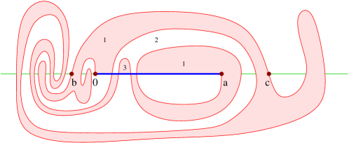
Figure 11: The lift of an $(\alpha,\beta)$-trace with $\widetilde{\rm w}\geq 0$.

Let $\Gamma$ be the set of connected components $\gamma$ of ${\widetilde{B}}\cap({\mathbb{R}}\times[0,\infty))$ such that the function $\widetilde{\rm w}$ is zero on one side of $\gamma$ and positive on the other. If $\gamma\in\Gamma$, neither end point of $\gamma$ can lie in the open interval $(0,a)$ since the function $\widetilde{\rm w}$ is at least one above this interval. We claim that there exists a connected component $\gamma\in\Gamma$ whose endpoints $b$ and $c$ satisfy

$$b\leq 0\leq a\leq c,\qquad{\partial}\gamma=\{b,c\}.$$ (42)

(See Figure 11.) To see this walk slightly above the real axis towards zero, starting at $-\infty$. Just before the first crossing $b_{1}$ with ${\widetilde{B}}$ turn left and follow the arc in ${\widetilde{B}}$ until it intersects the real axis again at $c_{1}$. The two intersections $b_{1}$ and $c_{1}$ are the endpoints of an element $\gamma_{1}$ of $\Gamma$. Obviously $b_{1}\leq 0$ and, as noted above, $c_{1}$ cannot lie in the interval $(0,a)$. For the same reason $c_{1}$ cannot be equal to zero. Hence either $c_{1}<0$ or $c_{1}\geq a$. In the latter case $\gamma_{1}$ is the required arc $\gamma$. In the former case we continue walking towards zero along the real axis until the next intersection with ${\widetilde{B}}$ and repeat the above procedure. Because the set of intersection points of ${\widetilde{B}}$ with ${\widetilde{\alpha}}={\mathbb{R}}$ is finite the process must terminate after finitely many steps. Thus we have proved the existence of an arc $\gamma\in\Gamma$ satisfying (42).

Assume that

$$c\geq b+1.$$

If $c=b+1$ then $c\in{\widetilde{\beta}}\cap({\widetilde{\beta}}+1)$ and hence ${\widetilde{\beta}}={\widetilde{\beta}}+1$. It follows that the intersection numbers of ${\mathbb{R}}$ and ${\widetilde{\beta}}$ at $b$ and $c$ agree. But this contradicts the fact that $b$ and $c$ are the endpoints of an arc in ${\widetilde{\beta}}$ contained in the closed upper halfplane. Thus we have $c>b+1.$ When this holds the arc $\gamma$ and its translate $\gamma+1$ must intersect and their intersection does not contain the endpoints $b$ and $c$. We denote by $\zeta\in\gamma\setminus\{b,c\}$ the first point in $\gamma+1$ we encounter when walking along $\gamma$ from $b$ to $c$. Let

$$U_{0}\subset{\widetilde{\beta}},\qquad U_{1}\subset{\widetilde{\beta}}+1$$

be sufficiently small connected open neighborhoods of $\zeta$, so that $\pi:U_{0}\to\beta$ and $\pi:U_{1}\to\beta$ are embeddings and their images agree. Thus

$$\pi(U_{0})=\pi(U_{1})\subset\beta$$

is an open neighborhood of $z:=\pi(\zeta)$ in $\beta$. Hence it follows from a lifting argument that $U_{0}=U_{1}\subset\gamma+1$ and this contradicts our choice of $\zeta$. This contradiction shows that our hypothesis $c\geq b+1$ must have been wrong. Thus we have proved that

$$b\leq 0\leq a\leq c<b+1\leq 1.$$

Hence $0\leq a<1$ and so $A=\pi([0,a])$ is an arc, as claimed. In the case $a=0$ we obtain the trivial arc from $x=y$ to itself. This proves (i).

We prove (ii). Assume that $\alpha$ and $\beta$ are noncontractible embedded circles. Then it follows from (i) that there exist oriented arcs $A\subset\alpha$ and $B\subset\beta$ from $x$ to $y$ such that $\nu_{\alpha}$ and $\nu_{\beta}$ are given by (40). If $x=y$ it follows also from (i) that $A=B=\{x\}$, hence

$$\nu_{\widetilde{\alpha}}\equiv 0,\qquad\nu_{\widetilde{\beta}}\equiv 0,$$

and hence $\widetilde{\rm w}\equiv 0$, in contradiction to our hypothesis. Thus $x\neq y$ and so $\Lambda$ satisfies the arc condition. This proves (ii) and Proposition 7.1. ∎

Example 7.2.

Let $\alpha\subset\Sigma$ be a noncontractible embedded circle and $\beta\subset\Sigma$ be a contractible embedded circle intersecting $\alpha$ transversally. Suppose $\beta$ is oriented as the boundary of an embedded disc $\Delta\subset\Sigma$. Let

$$x=y\in\alpha\cap\beta,\qquad\nu_{\alpha}\equiv 0,\qquad\nu_{\beta}\equiv 1,$$

and define

$${\rm w}(z):=\left\{\begin{array}[]{ll}1,&\mbox{for }z\in\Delta\setminus(\alpha\cup\beta),\\ 0,&\mbox{for }z\in\Sigma\setminus(\Delta\cup\alpha\cup\beta).\end{array}\right.$$

Then $\Lambda=(x,y,\nu_{\alpha},\nu_{\beta},{\rm w})$ is an $(\alpha,\beta)$-trace that satisfies the hypotheses of Proposition 7.1 (i) with $x=y$ and $A=\{x\}$.

Definition 7.3.

An $(\alpha,\beta)$-trace $\Lambda=(x,y,{\rm w})$ is called primitive if it satisfies the arc condition with boundary ${\partial}\Lambda=:(x,y,A,B)$ and

$$A\cap\beta=\alpha\cap B=\{x,y\}.$$

A smooth $(\alpha,\beta)$-lune $u$ is called primitive if its $(\alpha,\beta)$-trace $\Lambda_{u}$ is primitive. It is called embedded if $u:{\mathbb{D}}\to\Sigma$ is injective.

The next proposition is the special case of Theorems 6.7 and 6.8 for embedded lunes. It shows that isotopy classes of primitive smooth $(\alpha,\beta)$-lunes are in one-to-one correspondence with the simply connected components of $\Sigma\setminus(\alpha\cup\beta)$ with two corners. We will also call such a component a primitive $(\alpha,\beta)$-lune.

Proposition 7.4 (Embedded lunes).

Assume (H) and let $\Lambda=(x,y,{\rm w})$ be an $(\alpha,\beta)$-trace. The following are equivalent.

(i) $\Lambda$ is a combinatorial lune and its boundary ${\partial}\Lambda=(x,y,A,B)$ satisfies

$$A\cap B=\{x,y\}.$$

(ii) There exists an embedded $(\alpha,\beta)$-lune $u$ such that $\Lambda_{u}=\Lambda$.

If $\Lambda$ satisfies (i) then any two smooth $(\alpha,\beta)$-lunes $u$ and $v$ with $\Lambda_{u}=\Lambda_{v}=\Lambda$ are equivalent.

Proof.

We prove that (ii) implies (i). Let $u:{\mathbb{D}}\to\Sigma$ be an embedded $(\alpha,\beta)$-lune with $\Lambda_{u}=\Lambda$. Then $u|_{{\mathbb{D}}\cap{\mathbb{R}}}:{\mathbb{D}}\cap{\mathbb{R}}\to\alpha$ and $u|_{{\mathbb{D}}\cap S^{1}}:{\mathbb{D}}\cap S^{1}\to\beta$ are embeddings. Hence $\Lambda$ satisfies the arc condition and ${\partial}\Lambda=(x,y,A,B)$ with $A=u({\mathbb{D}}\cap{\mathbb{R}})$ and $B=u({\mathbb{D}}\cap S^{1})$. Since ${\rm w}$ is the counting function of $u$ it takes only the values zero and one. If $z\in A\cap B$ then $u^{-1}(z)$ contains a single point which must lie in ${\mathbb{D}}\cap{\mathbb{R}}$ and ${\mathbb{D}}\cap S^{1}$, hence is either $-1$ or $+1$, and so $z=x$ or $z=y$. The assertion about the intersection indices follows from the fact that $u$ is an immersion. Thus we have proved that (ii) implies (i).

We prove that (i) implies (ii). This relies on the following.

Claim. Let $\Lambda=(x,y,{\rm w})$ be an $(\alpha,\beta)$-trace that satisfies the arc condition and ${\partial}\Lambda=:(x,y,A,B)$ with ${A\cap B=\{x,y\}}$. Then $\Sigma\setminus(A\cup B)$ has two components and one of these is homeomorphic to the disc.

To prove the claim, let $\Gamma\subset\Sigma$ be an embedded circle obtained from $A\cup B$ by smoothing the corners. Then $\Gamma$ is contractible and hence, by a theorem of Epstein [8], bounds a disc. This proves the claim.

Now suppose that $\Lambda=(x,y,{\rm w})$ is an $(\alpha,\beta)$-trace that satisfies (i) and let ${\partial}\Lambda=:(x,y,A,B)$. By the claim, the complement $\Sigma\setminus(A\cup B)$ has two components, one of which is homeomorphic to the disc. Denote the components by $\Sigma_{0}$ and $\Sigma_{1}$. Since $\Lambda$ is a combinatorial lune, it follows that ${\rm w}$ only takes the values zero and one. Hence we may choose the indexing such that

$${\rm w}(z)=\left\{\begin{array}[]{ll}0,&\mbox{for }z\in\Sigma_{0}\setminus(\alpha\cup\beta),\\ 1,&\mbox{for }z\in\Sigma_{1}\setminus(\alpha\cup\beta).\end{array}\right.$$

We prove that $\Sigma_{1}$ is homeomorphic to the disc. Suppose, by contradiction, that $\Sigma_{1}$ is not homeomorphic to the disc. Then $\Sigma$ is not diffeomorphic to the $2$-sphere and, by the claim, $\Sigma_{0}$ is homeomorphic to the disc. By Definition 6.4, there is a smooth map $u:{\mathbb{D}}\to\Sigma$ that satisfies the boundary condition (33) such that $\Lambda_{u}=\Lambda$. Since $\Sigma$ is not diffeomorphic to the $2$-sphere, the homotopy class of $u$ is uniquely determined by the quadruple $(x,y,A,B)$ (see Theorem 2.4 above). Since $\Sigma_{0}$ is homeomorphic to the disc we may choose $u$ such that $u({\mathbb{D}})=\overline{\Sigma}_{0}$ and hence ${\rm w}(z)=\deg(u,z)=0$ for $z\in\Sigma_{1}\setminus(\alpha\cup\beta)$, in contradiction to our choice of indexing. This shows that $\Sigma_{1}$ must be homeomorphic to the disc. Let $N$ denote the closure of $\Sigma_{1}$:

$$N:=\overline{\Sigma}_{1}=\Sigma_{1}\cup A\cup B.$$

Then the orientation of ${\partial}N=A\cup B$ agrees with the orientation of $A$ and is opposite to the orientation of $B$, i.e. $N$ lies to the left of $A$ and to the right of $B$. Since the intersection index of $A$ and $B$ at $x$ is $+1$ and at $y$ is $-1$, it follows that the angles of $N$ at $x$ and $y$ are between zero and $\pi$ and hence $N$ is a $2$-manifold with two corners. Since $N$ is simply connected there exists a diffeomorphism $u:{\mathbb{D}}\to N$ such that

$$u(-1)=x,\qquad u(1)=y,\qquad u({\mathbb{D}}\cap{\mathbb{R}})=A,\qquad u({\mathbb{D}}\cap S^{1})=B.$$

This diffeomorphism is the required embedded $(\alpha,\beta)$-lune.

We prove that the embedded $(\alpha,\beta)$-lune in (ii) is unique up to equivalence. Let $v:{\mathbb{D}}\to\Sigma$ be another smooth $(\alpha,\beta)$-lune such that $\Lambda_{v}=\Lambda$. Then $v$ maps the boundary of ${\mathbb{D}}$ bijectively onto $A\cup B$, because $A\cap B=\{x,y\}$. Moreover, ${\rm w}$ is the counting function of $v$ and $\#v^{-1}(z)$ is constant on each component of $\Sigma\setminus(A\cup B)$. Hence $\#v^{-1}(z)=0$ for $z\in\Sigma_{0}$ and $\#v^{-1}(z)=1$ for $z\in\Sigma_{1}$. This shows that $v$ is injective and $v({\mathbb{D}})=N=u({\mathbb{D}}).$ Since $u$ and $v$ are embeddings the composition ${\varphi}:=u^{-1}\circ v:{\mathbb{D}}\to{\mathbb{D}}$ is an orientation preserving diffeomorphism such that ${\varphi}(\pm 1)=\pm 1$. Hence $v=u\circ{\varphi}$ is equivalent to $u$. This proves Proposition 7.4. ∎

Lemma 7.5.

Assume (H) and let $u:{\mathbb{D}}\to\Sigma$ be a smooth $(\alpha,\beta)$-lune.

(i) Let $S$ be a connected component of $\Sigma\setminus(\alpha\cup\beta)$. If $S\cap u({\mathbb{D}})\neq\emptyset$ then $S\subset u({\mathbb{D}})$ and $S$ is diffeomorphic to the open unit disc in ${\mathbb{C}}$.

(ii) Let $\Delta$ be a connected component of ${\mathbb{D}}\setminus u^{-1}(\alpha\cup\beta)$. Then $\Delta$ is diffeomorphic to the open unit disc and the restriction of $u$ to $\Delta$ is a diffeomorphism onto the open set $S:=u(\Delta)\subset\Sigma$.

Proof.

That $S\cap u({\mathbb{D}})\neq\emptyset$ implies $S\subset u({\mathbb{D}})$ follows from the fact that $u$ is an immersion. That this implies that $S$ is diffeomorphic to the open unit disc in ${\mathbb{C}}$ follows as in Proposition 6.12. This proves (i). By (i) the open set $S:=u(\Delta)$ in (ii) is diffeomorphic to the disc and hence is simply connected. Since $u:\Delta\to S$ is a proper covering it follows that $u:\Delta\to S$ is a diffeomorphism. This proves Lemma 7.5. ∎

Let $u:{\mathbb{D}}\to\Sigma$ be a smooth $(\alpha,\beta)$-lune. The image under $u$ of the connected component of ${\mathbb{D}}\setminus u^{-1}(\alpha\cup\beta)$ whose closure contains $-1$ is called the left end of $u$. The image under $u$ of the connected component of ${\mathbb{D}}\setminus u^{-1}(\alpha\cup\beta)$ whose closure contains $+1$ is called the right end of $u$.

Lemma 7.6.

Assume (H) and let $u$ be a smooth $(\alpha,\beta)$-lune. If there is a primitive $(\alpha,\beta)$-lune with the same left or right end as $u$ it is equivalent to $u$.

Proof.

If $u$ is not a primitive lune its ends have at least three corners. To see this, walk along ${\mathbb{D}}\cap{\mathbb{R}}$ (respectively ${\mathbb{D}}\cap S^{1}$) from $-1$ to $1$ and let $z_{0}$ (respectively $z_{1}$) be the first intersection point with $u^{-1}(\beta)$ (respectively $u^{-1}(\alpha)$). Then $u(-1)$, $u(z_{0})$, $u(z_{1})$ are corners of the left end of $u$. Hence the hypotheses of Lemma 7.6 imply that $u$ is a primitive lune. Two primitive lunes with the same ends are equivalent by Proposition 7.4. This proves Lemma 7.6. ∎

Proposition 7.7.

Assume (H) and suppose that $\Sigma$ is diffeomorphic to the $2$-sphere. If $u$ is a smooth $(\alpha,\beta)$-lune then $\Lambda_{u}$ satisfies the arc condition.

Proof.

The proof is by induction on the number of intersection points of $\alpha$ and $\beta$. It has three steps.

Step 1. Let $u$ be a smooth $(\alpha,\beta)$-lune whose $(\alpha,\beta)$-trace

$$\Lambda=\Lambda_{u}=(x,y,{\rm w})$$

does not satisfy the arc condition. Suppose there is a primitive $(\alpha,\beta)$-lune with endpoints in $\Sigma\setminus\{x,y\}$. Then there is an embedded loop $\beta^{\prime}$, isotopic to $\beta$ and transverse to $\alpha$, and a smooth $(\alpha,\beta^{\prime})$-lune $u^{\prime}$ with endpoints $x,y$ such that $\Lambda_{u^{\prime}}$ does not satisfy the arc condition and $\#(\alpha\cap\beta^{\prime})<\#(\alpha\cap\beta)$.

By Proposition 7.4, there exists a primitive smooth $(\alpha,\beta)$-lune $u_{0}:{\mathbb{D}}\to\Sigma$ whose endpoints $x_{0}:=u_{0}(-1)$ and $y_{0}:=u_{0}(+1)$ are contained in $\Sigma\setminus\{x,y\}$. Use this lune to remove the intersection points $x_{0}$ and $y_{0}$ by an isotopy of $\beta$, supported in a small neighborhood of the image of $u_{0}$. More precisely, extend $u_{0}$ to an embedding (still denoted by $u_{0}$) of the open set

$${\mathbb{D}}_{\varepsilon}:=\{z\in{\mathbb{C}}\,|\,{\rm Im}\,z>-{\varepsilon},|z|<1+{\varepsilon}\}$$

for ${\varepsilon}>0$ sufficiently small such that

$$u_{0}({\mathbb{D}}_{\varepsilon})\cap\beta=u_{0}({\mathbb{D}}_{\varepsilon}\cap S^{1}),\qquad u_{0}({\mathbb{D}}_{\varepsilon})\cap\alpha=u_{0}({\mathbb{D}}_{\varepsilon}\cap{\mathbb{R}}).$$

Choose a smooth cutoff function $\rho:{\mathbb{D}}_{\varepsilon}\to[0,1]$ which vanishes near the boundary and is equal to one on ${\mathbb{D}}$. Consider the vector field $\xi$ on $\Sigma$ that vanishes outside $u_{0}({\mathbb{D}}_{\varepsilon})$ and satisfies

$$u_{0}^{*}\xi(z)=-\rho(z){\mathbf{i}}.$$

Let $\psi_{t}:\Sigma\to\Sigma$ be the isotopy generated by $\xi$ and, for $T>0$ sufficiently large, define

$$\beta^{\prime}:=\psi_{T}(\beta),\qquad\Lambda^{\prime}:=(x,y,\nu_{\alpha},\nu_{\beta^{\prime}},{\rm w}^{\prime}).$$

Here $\nu_{\beta^{\prime}}:\beta^{\prime}\setminus\alpha\to{\mathbb{Z}}$ is the unique one-chain equal to $\nu_{\beta}$ on $\beta\setminus u_{0}({\mathbb{D}}_{\varepsilon})$ and ${\rm w}^{\prime}:\Sigma\setminus(\alpha\cup\beta^{\prime})\to{\mathbb{Z}}$ is the unique two-chain equal to ${\rm w}$ on $\Sigma\setminus u_{0}({\mathbb{D}}_{\varepsilon})$. Since $\Lambda$ does not satisfy the arc condition, neither does $\Lambda^{\prime}$. Let $U\subset{\mathbb{D}}$ be the union of the components of $u^{-1}(u_{0}({\mathbb{D}}_{\varepsilon}))$ that contain an arc in ${\mathbb{D}}\cap S^{1}$ and define the map $u^{\prime}:{\mathbb{D}}\to\Sigma$ by

$$u^{\prime}(z):=\left\{\begin{array}[]{rl}\psi_{T}(u(z)),&\mbox{if }z\in U,\\ u(z),&\mbox{if }z\in{\mathbb{D}}\setminus U.\end{array}\right.$$

We prove that $U\cap{\mathbb{R}}=\emptyset$. To see this, note that the restriction of $u$ to each connected component of $U$ is a diffeomorphism onto its image which is either equal to $u_{0}(\{z\in{\mathbb{D}}_{\varepsilon}\,|\,\left|z\right|\geq 1\})$ or equal to $u_{0}(\{z\in{\mathbb{D}}_{\varepsilon}\,|\,\left|z\right|\leq 1\})$ (see Figure 16 below). Thus

$$u(U)\cap(\alpha\setminus\{x_{0},y_{0}\})\subset\mathrm{int}(u(U))$$

and hence $U\cap{\mathbb{R}}=\emptyset$ as claimed. This implies that $u^{\prime}$ is a smooth $(\alpha,\beta^{\prime})$-lune such that ${\Lambda_{u^{\prime}}=\Lambda^{\prime}}$. Hence $\Lambda_{u^{\prime}}$ does not satisfy the arc condition. This proves Step 1.

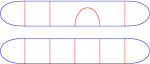
Figure 12: $\alpha$ encircles at least two primitive lunes.

Step 2. Let $u$ be a smooth $(\alpha,\beta)$-lune with endpoints $x,y$ and suppose that every primitive $(\alpha,\beta)$-lune has $x$ or $y$ as one of its endpoints. Then $\Lambda_{u}$ satisfies the arc condition.

Both connected components of $\Sigma\setminus\alpha$ are discs, and each of these discs contains at least two primitive $(\alpha,\beta)$-lunes. If it contains more than two there is one with endpoints in $\Sigma\setminus\{x,y\}$. Hence, under the assumptions of Step 2, each connected component of $\Sigma\setminus\alpha$ contains precisely two primitive $(\alpha,\beta)$-lunes. (See Figure 12.) Thus each connected component of $\Sigma\setminus(\alpha\cup\beta)$ is either a quadrangle or a primitive $(\alpha,\beta)$-lune and there are precisely four primitive $(\alpha,\beta)$-lunes, two in each connected component of $\Sigma\setminus\alpha$. At least two primitive $(\alpha,\beta)$-lunes contain $x$ and at least two contain $y$. (See Figure 13.)

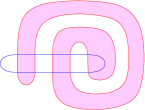
Figure 13: Four primitive lunes in the 2-sphere.

As $\Sigma$ is diffeomorphic to $S^{2}$, the number of intersection points of $\alpha$ and $\beta$ is even. Write $\alpha\cap\beta=\{x_{0},\dots,x_{2n-1}\},$ where the ordering is chosen along $\alpha$, starting at $x_{0}=x$. Then $x_{0}$ is contained in two primitive $(\alpha,\beta)$-lunes, one with endpoints $x_{0},x_{2n-1}$ and one with endpoints $x_{0},x_{1}$. Each connected component of $\Sigma\setminus\alpha$ determines an equivalence relation on $\alpha\cap\beta$: distinct points are equivalent iff they are connected by a $\beta$-arc in this component. Let $A$ be the connected component containing the $\beta$-arc from $x_{0}$ to $x_{2n-1}$ and $B$ be the connected component containing the $\beta$-arc from $x_{0}$ to $x_{1}$. Then $x_{j-1}\sim_{A}x_{2n-j}$ and $x_{j+1}\sim_{B}x_{2n-j}$ for $j=1,\dots,n$. Thus the only other intersection point contained in two primitive $(\alpha,\beta)$-lunes is $y=x_{n}$. Moreover, $\alpha$ and $\beta$ have opposite intersection indices at $x_{i}$ and $x_{i+1}$ for each $i$, because the arcs in $\alpha$ from $x_{i-1}$ to $x_{i}$ and from $x_{i}$ to $x_{i+1}$ are contained in different connected components of $\Sigma\setminus\beta$. Since $\alpha$ and $\beta$ have opposite intersection indices at $x$ and $y$ it follows that $n$ is odd. Now the image of a neighborhood of ${\mathbb{R}}\cap{\mathbb{D}}$ under $u$ is contained in either $\overline{A}$ or $\overline{B}$. Hence, when $n=2k+1\geq 3$, Figure 14 shows that one of the ends of $u$ is a quadrangle and the other end is a primitive $(\alpha,\beta)$-lune, in contradiction to Lemma 7.6. Hence the number of intersection points is $2n=2$, each component of $\Sigma\setminus(\alpha\cup\beta)$ is a primitive $(\alpha,\beta)$-lune, and all four primitive $(\alpha,\beta)$-lunes contain $x$ and $y$. By Lemma 7.6, one of them is equivalent to $u$. This proves Step 2.

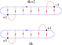
Figure 14: $\alpha$ intersects $\beta$ in $4k$ or $4k+2$ points.

Step 3. We prove the proposition.

Assume, by contradiction, that there is a smooth $(\alpha,\beta)$-lune $u$ such that $\Lambda_{u}$ does not satisfy the arc condition. By Step 1 we can reduce the number of intersection points of $\alpha$ and $\beta$ until there are no primitive $(\alpha,\beta)$-lunes with endpoints in $\Sigma\setminus\{x,y\}$. Once this algorithm terminates the resulting lune still does not satisfy the arc condition, in contradiction to Step 2. This proves Step 3 and Proposition 7.7. ∎

Proof of Theorem 6.5.

Let $u:{\mathbb{D}}\to\Sigma$ be a smooth $(\alpha,\beta)$-lune with $(\alpha,\beta)$-trace $\Lambda_{u}=:(x,y,{\rm w})$ and denote $A:=u({\mathbb{D}}\cap{\mathbb{R}})$ and $B:=u({\mathbb{D}}\cap S^{1})$. Since $u$ is an immersion, $\alpha$ and $\beta$ have opposite intersection indices at $x$ and $y$, and hence $x\neq y$. We must prove that $A$ and $B$ are arcs. It is obvious that $A$ is an arc whenever $\alpha$ is not compact, and $B$ is an arc whenever $\beta$ is not compact. It remains to show that $A$ and $B$ are arcs in the remaining cases. We prove this in four steps.

Step 1. If $\alpha$ is not a contractible embedded circle then $A$ is an arc.

This follows immediately from Proposition 7.1.

Step 2. If $\alpha$ and $\beta$ are contractible embedded circles then $A$ and $B$ are arcs.

If $\Sigma$ is diffeomorphic to $S^{2}$ this follows from Proposition 7.7. Hence assume that $\Sigma$ is not diffeomorphic to $S^{2}$. Then the universal cover of $\Sigma$ is diffeomorphic to the complex plane. Choose a universal covering $\pi:{\mathbb{C}}\to\Sigma$ and a point ${\widetilde{x}}\in\pi^{-1}(x).$ Choose lifts ${\widetilde{\alpha}},{\widetilde{\beta}}\subset{\mathbb{C}}$ of $\alpha,\beta$ such that ${\widetilde{x}}\in{\widetilde{\alpha}}\cap{\widetilde{\beta}}.$ Then ${\widetilde{\alpha}}$ and ${\widetilde{\beta}}$ are embedded loops in ${\mathbb{C}}$ and $u$ lifts to a smooth $({\widetilde{\alpha}},{\widetilde{\beta}})$-lune ${\widetilde{u}}:{\mathbb{D}}\to{\mathbb{C}}$ such that ${\widetilde{u}}(-1)={\widetilde{x}}.$ Compactify ${\mathbb{C}}$ to get the 2-sphere. Then, by Proposition 7.7, the subsets ${\widetilde{A}}:={\widetilde{u}}({\mathbb{D}}\cap{\mathbb{R}})\subset{\widetilde{\alpha}}$ and ${\widetilde{B}}:={\widetilde{u}}({\mathbb{D}}\cap S^{1})\subset{\widetilde{\beta}}$ are arcs. Since the restriction of $\pi$ to ${\widetilde{\alpha}}$ is a diffeomorphism from ${\widetilde{\alpha}}$ to $\alpha$ it follows that $A\subset\alpha$ is an arc. Similarly for $B$. This proves Step 2.

Step 3. If $\alpha$ is not a contractible embedded circle and $\beta$ is a contractible embedded circle then $A$ and $B$ are arcs.

That $A$ is an arc follows from Step 1. To prove that $B$ is an arc choose a universal covering $\pi:{\mathbb{C}}\to\Sigma$ with $\pi(0)=x$ and lifts ${\widetilde{\alpha}}$, ${\widetilde{\beta}}$, ${\widetilde{u}}$ with $0\in{\widetilde{\alpha}}\cap{\widetilde{\beta}}$ and ${\widetilde{u}}(-1)=0$ as in the proof of Step 2. Then ${\widetilde{\beta}}\subset{\mathbb{C}}$ is an embedded loop and we may assume without loss of generality that ${\widetilde{\alpha}}={\mathbb{R}}$ and ${\widetilde{A}}=[0,a]$ with $0<a<1$. (If $\alpha$ is a noncontractible embedded circle we choose the lift such that ${\widetilde{z}}\mapsto{\widetilde{z}}+1$ is a covering transformation and $\pi$ maps the interval $[0,1)$ bijectively onto $\alpha$; if $\alpha$ is not compact we choose the universal covering such that $\pi$ maps the interval $[0,a]$ bijectively onto $A$ and ${\widetilde{\beta}}$ is transverse to ${\mathbb{R}}$, and then replace ${\widetilde{\alpha}}$ by ${\mathbb{R}}$.) In the Riemann sphere $S^{2}\cong\overline{{\mathbb{C}}}={\mathbb{C}}\cup\{\infty\}$ the real axis ${\widetilde{\alpha}}={\mathbb{R}}$ compactifies to a great circle. Hence it follows from Proposition 7.7 that ${\widetilde{B}}$ is an arc. Since $\pi:{\widetilde{\beta}}\to\beta$ is a diffeomorphism it follows that $B$ is an arc. This proves Step 3.

Step 4. If $\beta$ is not a contractible embedded circle then $A$ and $B$ are arcs.

That $B$ is an arc follows from Step 1 by interchanging $\alpha$ and $\beta$ and replacing $u$ with the smooth $(\beta,\alpha)$-lune

$$v(z):=u\left(\frac{{\mathbf{i}}-z}{1-{\mathbf{i}}z}\right).$$

If $\alpha$ is not a contractible embedded circle then $A$ is an arc by Step 1. If $\alpha$ is a contractible embedded circle then $A$ is an arc by Step 3 with $\alpha$ and $\beta$ interchanged. This proves Step 4. The assertion of Theorem 6.5 follows from Steps 2, 3, and 4. ∎

8 Combinatorial Lunes

In this section we prove Theorems 6.7 and 6.8. Proposition 7.4 establishes the equivalence of (i) and (iii) in Theorem 6.7 under the additional hypothesis that $\Lambda=(x,y,A,B,{\rm w})$ satisfies the arc condition and $A\cap B=\{x,y\}$. In this case the hypothesis that $\Sigma$ is simply connected can be dropped. The induction argument for the proof of Theorems 6.7 and 6.8 is the content of the next three lemmas.

Lemma 8.1.

Assume (H) and suppose that $\Sigma$ is simply connected. Let $\Lambda=(x,y,{\rm w})$ be a combinatorial $(\alpha,\beta)$-lune with boundary ${\partial}\Lambda=(x,y,A,B)$ such that

$$A\cap B\neq\{x,y\}.$$

Then there exists a combinatorial $(\alpha,\beta)$-lune $\Lambda_{0}=(x_{0},y_{0},{\rm w}_{0})$ with boundary ${\partial}\Lambda_{0}=(x_{0},y_{0},A_{0},B_{0})$ such that ${\rm w}\geq{\rm w}_{0}$ and

$$A_{0}\subset A\setminus\{x,y\},\quad B_{0}\subset B\setminus\{x,y\},\quad A_{0}\cap B=A\cap B_{0}=\{x_{0},y_{0}\}.$$ (43)

Proof.

Let $\prec$ denote the order relation on $A$ determined by the orientation from $x$ to $y$. Denote the intersection points of $A$ and $B$ by

$$x=x_{0}\prec x_{1}\prec\cdots\prec x_{n-1}\prec x_{n}=y.$$

Define a function $\sigma:\{0,\dots,n-1\}\to\{1,\dots,n\}$ as follows. Walk along $B$ towards $y$, starting at $x_{i}$ and denote the next intersection point encountered by $x_{\sigma(i)}$. This function $\sigma$ is bijective. Let ${\varepsilon}_{i}\in\{\pm 1\}$ be the intersection index of $A$ and $B$ at $x_{i}$. Thus

$${\varepsilon}_{0}=1,\qquad{\varepsilon}_{n}=-1,\qquad\sum_{i=0}^{n}{\varepsilon}_{i}=0.$$

Consider the set

$$I:=\{i\in{\mathbb{N}}\,|\,0\leq i\leq n-1,\,{\varepsilon}_{i}=1,\,{\varepsilon}_{\sigma(i)}=-1\}.$$

We prove that this set has the following properties.

(a)

$I\neq\emptyset$.

(b)

If $i\in I$, $i<j<\sigma(i)$, and ${\varepsilon}_{j}=1$, then $j\in I$ and $i<\sigma(j)<\sigma(i)$.

(c)

If $i\in I$, $\sigma(i)<j<i$, and ${\varepsilon}_{j}=1$, then $j\in I$ and $\sigma(i)<\sigma(j)<i$.

(d)

$0\in I$ if and only if $n\in\sigma(I)$ if and only if $n=1=\sigma(0)$.

To see this, denote by $m_{i}$ the value of ${\rm w}$ in the right upper quadrant near $x_{i}$. Thus

$$m_{j}=m_{0}+\sum_{i=1}^{j}{\varepsilon}_{i}$$

for $j=1,\dots,n$ and

$$m_{\sigma(i)}=m_{i}+{\varepsilon}_{\sigma(i)}$$ (44)

for $i=0,\dots,n-1$. (See Figure 15.)

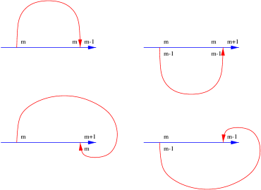
Figure 15: Simple arcs.

We prove that $I$ satisfies (a). Consider the sequence

$$i_{0}:=0,\qquad i_{1}:=\sigma(i_{0}),\qquad i_{2}:=\sigma(i_{1}),\dots.$$

Thus the points $x_{i}$ are encountered in the order

$$x=x_{0}=x_{i_{0}},x_{i_{1}},\dots,x_{i_{n-1}},x_{i_{n}}=x_{n}=y$$

when walking along $B$ from $x$ to $y$. By (44), we have

$${\varepsilon}_{i_{0}}=1,\qquad{\varepsilon}_{i_{n}}=-1,\qquad m_{i_{k}}=m_{i_{k-1}}+{\varepsilon}_{i_{k}}.$$

Let $k\in\{0,\dots,n-1\}$ be the largest integer such that ${\varepsilon}_{i_{k}}=1$. Then we have ${\varepsilon}_{\sigma(i_{k})}={\varepsilon}_{i_{k+1}}=-1$ and hence $i_{k}\in I$. Thus $I$ is nonempty.

We prove that $I$ satisfies (b) and (c). Let $i\in I$ such that $\sigma(i)>i$. Then ${\varepsilon}_{i}=1$ and ${\varepsilon}_{\sigma(i)}=-1$. Hence

$$m_{\sigma(i)}=m_{i}+{\varepsilon}_{\sigma(i)}=m_{i}-1,$$

and hence, in the interval $i<j<\sigma(i)$, the numbers of intersection points with positive and with negative intersection indices agree. Consider the arcs $A_{i}\subset A$ and $B_{i}\subset B$ that connect $x_{i}$ to $x_{\sigma(i)}$. Then $A\cap B_{i}=\{x_{i},x_{\sigma(i)}\}$. Since $\Sigma$ is simply connected the piecewise smooth embedded loop $A_{i}-B_{i}$ is contractible. This implies that the complement $\Sigma\setminus(A_{i}\cup B_{i})$ has two connected components. Let $\Sigma_{i}$ be the connected component of $\Sigma\setminus(A_{i}\cup B_{i})$ that contains the points slightly to the left of $A_{i}$. Then any arc on $B$ that starts at $x_{j}\in A_{i}$ with ${\varepsilon}_{j}=1$ is trapped in $\Sigma_{i}$ and hence must exit it through $A_{i}$. Hence

$$x_{j}\in A_{i},\quad{\varepsilon}_{j}=1\qquad\implies\qquad x_{\sigma(j)}\in A_{i},\quad{\varepsilon}_{\sigma(j)}=-1.$$

Thus we have proved that $I$ satisfies (b). That it satisfies (c) follows by a similar argument.

We prove that $I$ satisfies (d). Here we use the fact that $\Lambda$ satisfies (III) or, equivalently, $m_{0}=1$ and $m_{n}=0$. If $0\in I$ then $m_{\sigma(0)}=m_{0}+{\varepsilon}_{\sigma(0)}=0.$ Since $m_{i}>0$ for $i<n$ this implies $\sigma(0)=n=1$. Conversely, suppose that $n\in\sigma(I)$ and let $i:=\sigma^{-1}(n)\in I$. Then $m_{i}=m_{n}-{\varepsilon}_{\sigma(i)}=1.$ Since $m_{i}>1$ for $i\in I\setminus\{0\}$ this implies $i=0$. Thus $I$ satisfies (d).

It follows from (a), (b), and (c) by induction that there exists a point $i\in I$ such that $\sigma(i)\in\{i-1,i+1\}$. Assume first that $\sigma(i)=i+1$, denote by $A_{i}$ the arc in $A$ from $x_{i}$ to $x_{i+1}$, and denote by $B_{i}$ the arc in $B$ from $x_{i}$ to $x_{i+1}$. If $i=0$ it follows from (d) that $x_{i}=x_{0}=x$ and $x_{i+1}=x_{n}=y$, in contradiction to $A\cap B\neq\{x,y\}$. Hence $i\neq 0$ and it follows from (d) that $0<i<i+1<n.$ The arcs $A_{i}$ and $B_{i}$ satisfy

$$A_{i}\cap B=A\cap B_{i}=\{x_{i},x_{i+1}\}.$$

Let $D_{i}$ be the connected component of $\Sigma\setminus(A\cup B)$ that contains the points slightly to the left of $A_{i}$. This component is bounded by $A_{i}$ and $B_{i}$. Moreover, the function ${\rm w}$ is positive on $D_{i}$. Hence it follows from Propostion 6.12 that $D_{i}$ is diffeomorphic to the open unit disc in ${\mathbb{C}}$. Let ${\rm w}_{i}(z):=1$ for $z\in D_{i}$ and ${\rm w}_{i}(z):=0$ for $z\in\Sigma\setminus\overline{D}_{i}$. Then the combinatorial lune

$$\Lambda_{i}:=(x_{i},x_{i+1},A_{i},B_{i},{\rm w}_{i})$$

satisfies (43) and ${\rm w}_{i}\leq{\rm w}$.

Now assume $\sigma(i)=i-1$, denote by $A_{i}$ the arc in $A$ from $x_{i-1}$ to $x_{i}$, and denote by $B_{i}$ the arc in $B$ from $x_{i-1}$ to $x_{i}$. Thus the orientation of $A_{i}$ (from $x_{i-1}$ to $x_{i}$) agrees with the orientation of $A$ while the orientation of $B_{i}$ is opposite to the orientation of $B$. Moreover, we have $0<i-1<i<n.$ The arcs $A_{i}$ and $B_{i}$ satisfy

$$A_{i}\cap B=A\cap B_{i}=\{x_{i-1},x_{i}\}.$$

Let $D_{i}$ be the connected component of $\Sigma\setminus(A\cup B)$ that contains the points slightly to the left of $A_{i}$. This component is again bounded by $A_{i}$ and $B_{i}$, the function ${\rm w}$ is positive on $D_{i}$, and so $D_{i}$ is diffeomorphic to the open unit disc in ${\mathbb{C}}$ by Propostion 6.12. Let ${\rm w}_{i}(z):=1$ for $z\in D_{i}$ and ${\rm w}_{i}(z):=0$ for $z\in\Sigma\setminus\overline{D}_{i}$. Then the combinatorial lune

$$\Lambda_{i}:=(x_{i-1},x_{i},A_{i},B_{i},{\rm w}_{i})$$

satisfies (43) and ${\rm w}_{i}\leq{\rm w}$. This proves Lemma 8.1. ∎

Lemma 8.2.

Assume (H). Let $u$ be a smooth $(\alpha,\beta)$-lune whose $(\alpha,\beta)$-trace $\Lambda_{u}=(x,y,{\rm w})$ is a combinatorial $(\alpha,\beta)$-lune. Let $\gamma:[0,1]\to{\mathbb{D}}$ be a smooth path such that

$$\gamma(0)\in({\mathbb{D}}\cap{\mathbb{R}})\setminus\{\pm 1\},\quad\gamma(1)\in({\mathbb{D}}\cap S^{1})\setminus\{\pm 1\},\quad u(\gamma(t))\notin A$$

for $0<t<1$. Then ${\rm w}(u(\gamma(t)))=1$ for $t$ near $1$.

Proof.

Denote $A:=u({\mathbb{D}}\cap{\mathbb{R}})$. Since $\Lambda$ is a combinatorial $(\alpha,\beta)$-lune we have $x,y\notin u(\mathrm{int}({\mathbb{D}}))$. Hence $u^{-1}(A)$ is a union of embedded arcs, each connecting two points in ${\mathbb{D}}\cap S^{1}$. If ${\rm w}(u(\gamma(t))\geq 2$ for $t$ close to $1$, then $\gamma(1)\in{\mathbb{D}}\cap S^{1}$ is separated from ${\mathbb{D}}\cap{\mathbb{R}}$ by one these arcs in ${\mathbb{D}}\setminus{\mathbb{R}}$. This proves Lemma 8.2. ∎

For each combinatorial $(\alpha,\beta)$-lune $\Lambda$ the integer $\nu(\Lambda)$ denotes the number of equivalence classes of smooth $(\alpha,\beta)$-lunes $u$ with $\Lambda_{u}=\Lambda$.

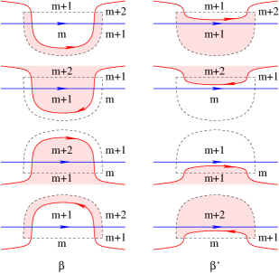
Figure 16: Deformation of a lune.

Lemma 8.3.

Assume (H) and suppose that $\Sigma$ is simply connected. Let $\Lambda=(x,y,{\rm w})$ be a combinatorial $(\alpha,\beta)$-lune with boundary ${\partial}\Lambda=(x,y,A,B)$ such that $A\cap B\neq\{x,y\}$. Then there exists an embedded loop $\beta^{\prime}$, isotopic to $\beta$ and transverse to $\alpha$, and a combinatorial $(\alpha,\beta^{\prime})$-lune $\Lambda^{\prime}=(x,y,{\rm w}^{\prime})$ with boundary ${\partial}\Lambda^{\prime}=(x,y,A,B^{\prime})$ such that

$$\#(A^{\prime}\cap B^{\prime})<\#(A\cap B),\qquad\nu(\Lambda)=\nu(\Lambda^{\prime}).$$

Proof.

By Lemma 8.1 there exists a combinatorial $(\alpha,\beta)$-lune

$$\Lambda_{0}=(x_{0},y_{0},{\rm w}_{0}),\qquad{\partial}\Lambda_{0}=(x_{0},y_{0},A_{0},B_{0}),$$

that satisfies ${\rm w}\geq{\rm w}_{0}$ and (43). In particular, we have

$$A_{0}\cap B_{0}=\{x_{0},y_{0}\}$$

and so, by Proposition 7.4, there is an embedded smooth lune $u_{0}:{\mathbb{D}}\to\Sigma$ with bottom boundary $A_{0}$ and top boundary $B_{0}$. As in the proof of Step 1 in Proposition 7.7 we use this lune to remove the intersection points $x_{0}$ and $y_{0}$ by an isotopy of $B$, supported in a small neighborhood of the image of $u_{0}$. This isotopy leaves the number $\nu(\Lambda)$ unchanged. More precisely, extend $u_{0}$ to an embedding (still denoted by $u_{0}$) of the open set

$${\mathbb{D}}_{\varepsilon}:=\{z\in{\mathbb{C}}\,|\,{\rm Im}\,z>-{\varepsilon},|z|<1+{\varepsilon}\}$$

for ${\varepsilon}>0$ sufficiently small such that

$$u_{0}({\mathbb{D}}_{\varepsilon})\cap B=u_{0}({\mathbb{D}}_{\varepsilon}\cap S^{1}),\qquad u_{0}({\mathbb{D}}_{\varepsilon})\cap A=u_{0}({\mathbb{D}}_{\varepsilon}\cap{\mathbb{R}}),$$

$$u(\{z\in{\mathbb{D}}_{\varepsilon}\,|\,|z|>1\})\cap\beta=\emptyset,\quad u(\{z\in{\mathbb{D}}_{\varepsilon}\,|\,{\rm Re}\,z<0\})\cap\alpha=\emptyset.$$

Choose a smooth cutoff function $\rho:{\mathbb{D}}_{\varepsilon}\to[0,1]$ that vanishes near the boundary of ${\mathbb{D}}_{\varepsilon}$ and is equal to one on ${\mathbb{D}}$. Consider the vector field $\xi$ on $\Sigma$ that vanishes outside $u_{0}({\mathbb{D}}_{\varepsilon})$ and satisfies

$$u_{0}^{*}\xi(z)=-\rho(z){\mathbf{i}}.$$

Let $\psi_{t}:\Sigma\to\Sigma$ be the isotopy generated by $\xi$ and, for $T>0$ sufficiently large, define

$$\beta^{\prime}:=\psi_{T}(\beta),\qquad B^{\prime}:=\psi_{T}(B),\qquad\Lambda^{\prime}:=(x,y,A,B^{\prime},{\rm w}^{\prime}),$$

where ${\rm w}^{\prime}:\Sigma\setminus(\alpha\cup\beta^{\prime})\to{\mathbb{Z}}$ is the unique two-chain that agrees with ${\rm w}$ on $\Sigma\setminus u_{0}({\mathbb{D}}_{\varepsilon})$. Thus ${\rm w}^{\prime}$ corresponds to the homotopy from $A$ to $B$ determined by ${\rm w}$ followed by the homotopy $\psi_{t}$ from $B$ to $B^{\prime}$. Then $\Lambda^{\prime}$ is a combinatorial $(\alpha,\beta^{\prime})$-lune. If $u:{\mathbb{D}}\to\Sigma$ is a smooth $(\alpha,\beta)$-lune let $U\subset{\mathbb{D}}$ be the unique component of $u^{-1}(u_{0}({\mathbb{D}}_{\varepsilon}))$ that contains an arc in ${\mathbb{D}}\cap S^{1}$. Then $U$ does not intersect ${\mathbb{D}}\cap{\mathbb{R}}$. (See Figure 16.) Hence the map $u^{\prime}:{\mathbb{D}}\to\Sigma$, defined by

$$u^{\prime}(z):=\left\{\begin{array}[]{rl}\psi_{T}(u(z)),&\mbox{if }z\in U,\\ u(z),&\mbox{if }z\in{\mathbb{D}}\setminus U,\end{array}\right.$$

is a smooth $(\alpha,\beta^{\prime})$-lune such that $\Lambda_{u^{\prime}}=\Lambda^{\prime}$.

We claim that the map $u\mapsto u^{\prime}$ defines a one-to-one correspondence between smooth $(\alpha,\beta)$-lunes $u$ such that $\Lambda_{u}=\Lambda$ and smooth $(\alpha,\beta^{\prime})$-lunes $u^{\prime}$ such that $\Lambda_{u^{\prime}}=\Lambda^{\prime}$. The map $u\mapsto u^{\prime}$ is obviously injective. To prove that it is surjective we choose a smooth $(\alpha,\beta^{\prime})$-lune $u^{\prime}$ such that $\Lambda_{u^{\prime}}=\Lambda^{\prime}$. Denote by

$$U^{\prime}\subset{\mathbb{D}}$$

the unique connected component of ${u^{\prime}}^{-1}(u_{0}({\mathbb{D}}_{\varepsilon}))$ that contains an arc in ${\mathbb{D}}\cap S^{1}$. There are four cases as depicted in Figure 16. In two of these cases (second and third row) we have $u^{\prime}(U^{\prime})\cap\alpha=\emptyset$ and hence $U^{\prime}\cap{\mathbb{R}}=\emptyset$. In the casees where $u^{\prime}(U^{\prime})\cap\alpha\neq\emptyset$ it follows from an orientation argument (fourth row) and from Lemma 8.2 (first row) that $U^{\prime}$ cannot intersect ${\mathbb{D}}\cap{\mathbb{R}}$. Thus we have shown that $U^{\prime}$ does not intersect ${\mathbb{D}}\cap{\mathbb{R}}$ in all four cases. This implies that $u^{\prime}$ is in the image of the map $u\mapsto u^{\prime}$. Hence the map $u\mapsto u^{\prime}$ is bijective as claimed, and hence

$$\nu(\Lambda)=\nu(\Lambda^{\prime}).$$

This proves Lemma 8.3. ∎

Proof of Theorems 6.7 and 6.8.

Assume first that $\Sigma$ is simply connected. We prove that (iii) implies (i) in Theorem 6.7. Let $\Lambda$ be a combinatorial $(\alpha,\beta)$-lune. By Lemma 8.3, reduce the number of intersection points of $\Lambda$, while leaving the number $\nu(\Lambda)$ unchanged. Continue by induction until reaching an embedded combinatorial lune in $\Sigma$. By Proposition 7.4, such a lune satisfies $\nu=1$. Hence $\nu(\Lambda)=1$. In other words, there is a smooth $(\alpha,\beta)$-lune $u:{\mathbb{D}}\to\Sigma$, unique up to equivalence, such that $\Lambda_{u}=\Lambda$. Thus we have proved that (iii) implies (i). We have also proved, in the simply connected case, that $u$ is uniquely determined by $\Lambda_{u}$ up to equivalence. From now on we drop the hypothesis that $\Sigma$ is simply connected.

We prove Theorem 6.8. Let $u:{\mathbb{D}}\to\Sigma$ and $u^{\prime}:{\mathbb{D}}\to\Sigma$ be smooth $(\alpha,\beta)$-lunes such that

$$\Lambda_{u}=\Lambda_{u^{\prime}}.$$

Let ${\widetilde{u}}:{\mathbb{D}}\to{\widetilde{\Sigma}}$ and ${\widetilde{u}}^{\prime}:{\mathbb{D}}\to{\widetilde{\Sigma}}$ be lifts to the universal cover such that

$${\widetilde{u}}(-1)={\widetilde{u}}^{\prime}(-1).$$

Then $\Lambda_{{\widetilde{u}}}=\Lambda_{{\widetilde{u}}^{\prime}}$. Hence, by what we have already proved, ${\widetilde{u}}$ is equivalent to ${\widetilde{u}}^{\prime}$ and hence $u$ is equivalent to $u^{\prime}$. This proves Theorem 6.8.

We prove that (i) implies (ii) in Theorem 6.7. Let $u:{\mathbb{D}}\to\Sigma$ be a smooth $(\alpha,\beta)$-lune and denote by $\Lambda_{u}=:(x,y,A,B,{\rm w})$ be its $(\alpha,\beta)$-trace. Then ${\rm w}(z)=\#u^{-1}(z)$ is the counting function of $u$ and hence is nonnegative. For $0<t\leq 1$ define the curve $\lambda_{t}:[0,1]\to{\mathbb{R}\mathrm{P}}^{1}$ by

$$du(-\cos(\pi s),t\sin(\pi s))\lambda_{t}(s):={\mathbb{R}}\frac{{\partial}}{{\partial}s}u(-\cos(\pi s),t\sin(\pi s)),\quad 0\leq s\leq 1.$$

For $t=0$ use the same definition for $0<s<1$ and extend the curve continuously to the closed interval $0\leq s\leq 1$. Then

$$\begin{split}\lambda_{0}(s)&=du(-\cos(\pi s),0)^{-1}T_{u(-\cos(\pi s),0)}\alpha,\\ \lambda_{1}(s)&=du(-\cos(\pi s),\sin(\pi s))^{-1}T_{u(-\cos(\pi s),\sin(\pi s))}\beta,\end{split}\qquad 0\leq s\leq 1.$$

The Viterbo–Maslov index $\mu(\Lambda_{u})$ is, by definition, the relative Maslov index of the pair of Lagrangian paths $(\lambda_{0},\lambda_{1})$, denoted by $\mu(\lambda_{0},\lambda_{1})$ (see Definition 3.1 above or [39, 30]). Hence it follows from the homotopy axiom for the relative Maslov index that

$$\mu(\Lambda_{u})=\mu(\lambda_{0},\lambda_{1})=\mu(\lambda_{0},\lambda_{t})$$

for every $t>0$. Choosing $t$ sufficiently close to zero we find that $\mu(\Lambda_{u})=1$.

We prove that (iii) implies (ii) in Theorem 6.7. If $\Lambda=(x,y,{\rm w})$ is a combinatorial $(\alpha,\beta)$-lune, then ${\rm w}\geq 0$ by (I) in Definition 6.6. Moreover, by the trace formula (37), we have

$$\mu(\Lambda)=\frac{m_{x}(\Lambda)+m_{y}(\Lambda)}{2}.$$

It follows from (II) and (III) in Definition 6.6 that $m_{x}(\Lambda)=m_{y}(\Lambda)=1$ and hence $\mu(\Lambda)=1$. Thus we have proved that (iii) implies (ii).

We prove that (ii) implies (iii) in Theorem 6.7. Let $\Lambda=(x,y,{\rm w})$ be an $(\alpha,\beta)$-trace such that ${\rm w}\geq 0$ and $\mu(\Lambda)=1$. Denote $\nu_{\alpha}:={\partial}{\rm w}|_{\alpha\setminus\beta}$ and $\nu_{\beta}:=-{\partial}{\rm w}|_{\beta\setminus\alpha}$. Reversing the orientation of $\alpha$ or $\beta$, if necessary, we may assume that $\nu_{\alpha}\geq 0$ and $\nu_{\beta}\geq 0$. Let ${\varepsilon}_{x},{\varepsilon}_{y}\in\{\pm 1\}$ be the intersection indices of $\alpha$ and $\beta$ at $x,y$ with these orientations, and let

$$n_{\alpha}:=\min\nu_{\alpha}\geq 0,\qquad n_{\beta}:=\min\nu_{\beta}\geq 0.$$

As before, denote by $m_{x}$ (respectively $m_{y}$) the sum of the four values of ${\rm w}$ encountered when walking along a small circle surrounding $x$ (respectvely $y$). Since the Viterbo–Maslov index of $\Lambda$ is odd, we have ${\varepsilon}_{x}\neq{\varepsilon}_{y}$ and thus $x\neq y$. This shows that $\Lambda$ satisfies the arc condition if and only if $n_{\alpha}=n_{\beta}=0$.

We prove that $\Lambda$ satisfies (II). Suppose, by contradiction, that $\Lambda$ does not satisfy (II). Then ${\varepsilon}_{x}=-1$ and ${\varepsilon}_{y}=1$. This implies that the values of ${\rm w}$ near $x$ are given by $k$, $k+n_{\alpha}+1$, $k+n_{\alpha}+n_{\beta}+1$, $k+n_{\beta}+1$ for some integer $k$. Since ${\rm w}\geq 0$ these numbers are all nonnegative. Hence $k\geq 0$ and hence $m_{x}\geq 3$. The same argument shows that $m_{y}\geq 3$ and, by the trace formula (37), we have $\mu(\Lambda)=(m_{x}(\Lambda)+m_{y}(\Lambda))/2\geq 3,$ in contradiction to our hypothesis. This shows that $\Lambda$ satisfies (II).

We prove that $\Lambda$ satisfies the arc condition and (III). By (II) we have ${\varepsilon}_{x}=1$. Hence the values of ${\rm w}$ near $x$ in counterclockwise order are given by $k_{x},$ $k_{x}+n_{\alpha}+1,$ $k_{x}+n_{\alpha}-n_{\beta},$ $k_{x}-n_{\beta}$ for some integer $k_{x}\geq n_{\beta}\geq 0$. This implies

$$m_{x}(\Lambda)=4k_{x}-2n_{\beta}+2n_{\alpha}+1$$

and, similarly, $m_{y}(\Lambda)=4k_{y}-2n_{\beta}+2n_{\alpha}+1$ for some integer $k_{y}\geq n_{\beta}\geq 0$. Hence, by the trace formula (37), we have

$$1=\mu(\Lambda)=\frac{m_{x}(\Lambda)+m_{y}(\Lambda)}{2}=k_{x}+(k_{x}-n_{\beta})+k_{y}+(k_{y}-n_{\beta})+2n_{\alpha}+1.$$

Hence $k_{x}=k_{y}=n_{\alpha}=n_{\beta}=0$ and so $\Lambda$ satisfies the arc condition and (III). Thus we have shown that (ii) implies (i). This proves Theorem 6.7. ∎

Example 8.4.

The arguments in the proof of Theorem 6.7 can be used to show that, if $\Lambda$ is an $(\alpha,\beta)$-trace with $\mu(\Lambda)=1,$ then (I)$\implies$(III)$\implies$(II). Figure 17 shows three $(\alpha,\beta)$-traces that satisfy the arc condition and have Viterbo–Maslov index one but do not satisfy (I); one that still satisfies (II) and (III), one that satisfies (II) but not (III), and one that satisfies neither (II) nor (III). Figure 18 shows an $(\alpha,\beta)$-trace of Viterbo–Maslov index two that satisfies (I) and (III) but not (II). Figure 19 shows an $(\alpha,\beta)$-trace of Viterbo–Maslov index three that satisfies (I) and (II) but not (III).

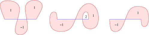
Figure 17: Three $(\alpha,\beta)$-traces with Viterbo–Maslov index one.

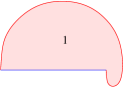
Figure 18: An $(\alpha,\beta)$-trace with Viterbo–Maslov index two.

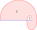
Figure 19: An $(\alpha,\beta)$-trace with Viterbo–Maslov index three.

We close this section with two results about lunes that will be useful below.

Proposition 8.5.

Assume (H) and suppose that $\alpha$ and $\beta$ are noncontractible nonisotopic transverse embedded circles and let $x,y\in\alpha\cap\beta.$ Then there is at most one $(\alpha,\beta)$-trace from $x$ to $y$ that satisfies the arc condition. Hence, by Theorems 6.5 and 6.8, there is at most one equivalence class of smooth $(\alpha,\beta)$-lunes from $x$ to $y$.

Proof.

Let

$$\alpha=\alpha_{1}\cup\alpha_{2},\qquad\beta=\beta_{1}\cup\beta_{2},$$

where $\alpha_{1}$ and $\alpha_{2}$ are the two arcs of $\alpha$ with endpoints $x$ and $y$, and similarly for $\beta$. Assume that the quadruple $(x,y,\alpha_{1},\beta_{1})$ is an $(\alpha,\beta)$-trace. Then $\alpha_{1}$ is homotopic to $\beta_{1}$ with fixed endpoints. Since $\alpha$ is not contractible, $\alpha_{2}$ is not homotopic to $\beta_{1}$ with fixed endpoints. Since $\beta$ is not contractible, $\beta_{2}$ is not homotopic to $\alpha_{1}$ with fixed endpoints. Since $\alpha$ is not isotopic to $\beta$, $\alpha_{2}$ is not homotopic to $\beta_{2}$ with fixed endpoints. Hence the quadruple $(x,y,\alpha_{i},\beta_{j})$ is not an $(\alpha,\beta)$-trace unless $i=j=1$. This proves Proposition 8.5. ∎

The hypotheses that the loops $\alpha$ and $\beta$ are not contractible and not isotopic to each other cannot be removed in Proposition 8.5. A pair of isotopic circles with precisely two intersection points is an example. Another example is a pair consisting of a contractible and a non-contractible loop, again with precisely two intersection points.

Proposition 8.6.

Assume (H). If there is a smooth $(\alpha,\beta)$-lune then there is a primitive $(\alpha,\beta)$-lune.

Proof.

The proof has three steps.

Step 1. If $\alpha$ or $\beta$ is a contractible embedded circle and $\alpha\cap\beta\neq\emptyset$ then there exists a primitive $(\alpha,\beta)$-lune.

Assume $\alpha$ is a contractible embedded circle. Then, by a theorem of Epstein [9], there exists an embedded closed disc $D\subset\Sigma$ with boundary ${\partial}D=\alpha$. Since $\alpha$ and $\beta$ intersect transversally, the set $D\cap\beta$ is a finite union of arcs. Let ${\mathcal{A}}$ be the set of all arcs $A\subset\alpha$ which connect the endpoints of an arc $B\subset D\cap\beta$. Then ${\mathcal{A}}$ is a nonempty finite set, partially ordered by inclusion. Let $A_{0}\subset\alpha$ be a minimal element of ${\mathcal{A}}$ and $B_{0}\subset D\cap\beta$ be the arc with the same endpoints as $A_{0}$. Then $A_{0}$ and $B_{0}$ bound a primitive $(\alpha,\beta)$-lune. This proves Step 1 when $\alpha$ is a contractible embedded circle. When $\beta$ is a contractible embedded circle the proof is analogous.

Step 2. Assume $\alpha$ and $\beta$ are not contractible embedded circles. If there exists a smooth $(\alpha,\beta)$-lune then there exists an embedded $(\alpha,\beta)$-lune $u$ such that $u^{-1}(\alpha)={\mathbb{D}}\cap{\mathbb{R}}$.

Let $v:{\mathbb{D}}\to\Sigma$ be a smooth $(\alpha,\beta)$-lune. Then the set

$$X:=v^{-1}(\alpha)\subset{\mathbb{D}}$$

is a smooth $1$-manifold with boundary ${\partial}X=v^{-1}(\alpha)\cap S^{1}.$ The interval ${\mathbb{D}}\cap{\mathbb{R}}$ is one component of $X$ and no component of $X$ is a circle. (If $X_{0}\subset X$ is a circle, then $v|_{X_{0}}:X_{0}\to\Sigma$ is a contractible loop covering $\alpha$ finitely many times. Hence, by Lemma A.3 in the appendix, it would follow that $\alpha$ is a contractible embedded circle, in contradiction to the hypothesis of Step 2.) Write

$${\partial}X=\{e^{{\mathbf{i}}\theta_{1}},\dots,e^{{\mathbf{i}}\theta_{n}}\},\qquad\pi=\theta_{1}>\theta_{2}>\cdots>\theta_{n-1}>\theta_{n}=0.$$

Then there is a permutation $\sigma\in S_{n}$ such that the arc of $v^{-1}(\alpha)$ that starts at $e^{{\mathbf{i}}\theta_{j}}$ ends at $e^{{\mathbf{i}}\theta_{\sigma(j)}}$. This permutation satisfies $\sigma\circ\sigma={\rm id}$, $\sigma(1)=n$, and

$$j<k<\sigma(j)\qquad\implies\qquad j<\sigma(k)<\sigma(j).$$

Hence, by induction, there exists a $j\in\{1,\dots,n-1\}$ such that $\sigma(j)=j+1$. Let $X_{0}\subset X$ be the submanifold with boundary points $e^{{\mathbf{i}}\theta_{j}}$ and $e^{{\mathbf{i}}\theta_{j+1}}$ and denote

$$Y_{0}:=\left\{e^{{\mathbf{i}}\theta}\,|\,\theta_{j+1}\leq\theta\leq\theta_{j}\right\}.$$

Then the closure of the domain $\Delta\subset{\mathbb{D}}$ bounded by $X_{0}$ and $Y_{0}$ is diffeomorphic to the half disc and $\overline{\Delta}\cap v^{-1}(\alpha)=X_{0}$. Hence there exists an orientation preserving embedding ${\varphi}:{\mathbb{D}}\to{\mathbb{D}}$ that maps ${\mathbb{D}}\cap{\mathbb{R}}$ onto $X_{0}$ and maps ${\mathbb{D}}\cap S^{1}$ onto $Y_{0}$. It follows that

$$u:=v\circ{\varphi}:{\mathbb{D}}\to\Sigma$$

is a smooth $(\alpha,\beta)$-lune such that

$$u^{-1}(\alpha)={\varphi}^{-1}(\overline{\Delta}\cap v^{-1}(\alpha))={\varphi}^{-1}(X_{0})={\mathbb{D}}\cap{\mathbb{R}}.$$

Moreover, $\Lambda_{u}=(x,y,A,B,{\rm w})$ with

$$x:=v(e^{{\mathbf{i}}\theta_{j}}),\qquad y:=v(e^{{\mathbf{i}}\theta_{j+1}}),\qquad A:=v(X_{0}),\qquad B:=v(Y_{0}).$$

Since $A\cap B=\alpha\cap B=\{x,y\}$, it follows from Proposition 7.4 that $u$ is an embedding. This proves Step 2.

Step 3. Assume $\alpha$ and $\beta$ are not contractible embedded circles. If there exists an embedded $(\alpha,\beta)$-lune $u$ such that $u^{-1}(\alpha)={\mathbb{D}}\cap{\mathbb{R}}$ then there exists a primitive $(\alpha,\beta)$-lune.

Repeat the argument in the proof of Step 2 with $v$ replaced by $u$ and the set $v^{-1}(\alpha)$ replaced by the $1$-manifold

$$Y:=u^{-1}(\beta)\subset{\mathbb{D}}$$

with boundary

$${\partial}Y=u^{-1}(\beta)\cap{\mathbb{R}}.$$

The argument produces an arc $Y_{0}\subset Y$ with boundary points $a<b$ such that the closed interval ${X_{0}:=[a,b]}$ intersects $Y$ only in the endpoints. Hence the arcs $A_{0}:=u(X_{0})$ and ${B_{0}:=u(Y_{0})}$ bound a primitive $(\alpha,\beta)$-lune. This proves Step 3 and Proposition 8.6. ∎

III. Floer Homology

9 Combinatorial Floer Homology

We assume throughout this section that $\Sigma$ is an oriented 2-manifold without boundary and that $\alpha,\beta\subset\Sigma$ are noncontractible nonisotopic transverse embedded circles. We orient $\alpha$ and $\beta$. There are three ways we can count the number of points in their intersection:

• The numerical intersection number ${\mathrm{num}\left(\alpha,\beta\right)}$ is the actual number of intersection points.

• The geometric intersection number ${\mathrm{geo}\left(\alpha,\beta\right)}$ is defined as the minimum of the numbers ${\mathrm{num}\left(\alpha,\beta^{\prime}\right)}$ over all embedded loops $\beta^{\prime}$ that are transverse to $\alpha$ and isotopic to $\beta$.

• The algebraic intersection number ${\mathrm{alg}\left(\alpha,\beta\right)}$ is the sum

  $$\alpha\cdot\beta=\sum_{x\in\alpha\cap\beta}\pm 1$$

  where the plus sign is chosen iff the orientations match in the direct sum $T_{x}\Sigma=T_{x}\alpha\oplus T_{x}\beta.$

Note that $\left|{\mathrm{alg}\left(\alpha,\beta\right)}\right|\leq{\mathrm{geo}\left(\alpha,\beta\right)}\leq{\mathrm{num}\left(\alpha,\beta\right)}.$

Theorem 9.1.

Define a chain complex ${\partial}:{\mathrm{CF}}(\alpha,\beta)\to{\mathrm{CF}}(\alpha,\beta)$ by

$${\mathrm{CF}}(\alpha,\beta)=\bigoplus_{x\in\alpha\cap\beta}{\mathbb{Z}}_{2}x,\qquad{\partial}x=\sum_{y}n(x,y)y,$$ (45)

where $n(x,y)$ denotes the number modulo two of equivalence classes of smooth $(\alpha,\beta)$-lunes from $x$ to $y$. Then

$${\partial}\circ{\partial}=0.$$

The homology group of this chain complex is denoted by

$${\mathrm{HF}}(\alpha,\beta):=\ker{\partial}/{\rm im}{\partial}$$

and is called the Combinatorial Floer Homology of the pair $(\alpha,\beta)$.

Proof.

See Section 10 page 10. ∎

Theorem 9.2.

Combinatorial Floer homology is invariant under isotopy: If $\alpha^{\prime},\beta^{\prime}\subset\Sigma$ are noncontractible transverse embedded circles such that $\alpha$ is isotopic to $\alpha^{\prime}$ and $\beta$ is isotopic to $\beta^{\prime}$ then

$${\mathrm{HF}}(\alpha,\beta)\cong{\mathrm{HF}}(\alpha^{\prime},\beta^{\prime}).$$

Proof.

See Section 11 page 11. ∎

Theorem 9.3.

Combinatorial Floer homology is isomorphic to the original analytic Floer homology. In fact, the two chain complexes agree.

Proof.

See Section 12 page 12. ∎

Corollary 9.4.

If ${\mathrm{geo}\left(\alpha,\beta\right)}={\mathrm{num}\left(\alpha,\beta\right)}$ there is no smooth $(\alpha,\beta)$-lune.

Proof.

If there exists a smooth $(\alpha,\beta)$-lune then, by Proposition 8.6, there exists a primitive $(\alpha,\beta)$-lune and hence there exists an embedded curve $\beta^{\prime}$ that is isotopic to $\beta$ and satisfies ${\mathrm{num}\left(\alpha,\beta^{\prime}\right)}<{\mathrm{num}\left(\alpha,\beta\right)}$. This contradicts our hypothesis. ∎

Corollary 9.5.

$\dim{\mathrm{HF}}(\alpha,\beta)={\mathrm{geo}\left(\alpha,\beta\right)}$.

Proof.

By Theorem 9.2 we may assume that ${\mathrm{num}\left(\alpha,\beta\right)}={\mathrm{geo}\left(\alpha,\beta\right)}$. In this case there is no $(\alpha,\beta)$-lune by Corollary 9.4. Hence the Floer boundary operator is zero, and hence the dimension of

$${\mathrm{HF}}(\alpha,\beta)\cong{\mathrm{CF}}(\alpha,\beta)$$

is the geometric intersection number ${\mathrm{geo}\left(\alpha,\beta\right)}$. ∎

Corollary 9.6.

If ${\mathrm{geo}\left(\alpha,\beta\right)}<{\mathrm{num}\left(\alpha,\beta\right)}$ there is a primitive $(\alpha,\beta)$-lune.

Proof.

By Corollary 9.5, the Floer homology group has dimension

$$\dim\,{\mathrm{HF}}(\alpha,\beta)={\mathrm{geo}\left(\alpha,\beta\right)}.$$

Since the Floer chain complex has dimension

$$\dim\,{\mathrm{CF}}(\alpha,\beta)={\mathrm{num}\left(\alpha,\beta\right)}$$

it follows that the Floer boundary operator is nonzero. Hence there exists a smooth $(\alpha,\beta)$-lune and hence, by Proposition 8.6, there exists a primitive $(\alpha,\beta)$-lune. ∎

Remark 9.7 (Action Filtration).

Consider the space

$${\Omega}_{\alpha,\beta}:=\left\{x\in C^{\infty}([0,1],\Sigma)\,|\,x(0)\in\alpha,\,x(1)\in\beta\right\}$$

of paths connecting $\alpha$ to $\beta$. Every intersection point $x\in\alpha\cap\beta$ determines a constant path in ${\Omega}_{\alpha,\beta}$ and hence a component of ${\Omega}_{\alpha,\beta}$. In general, ${\Omega}_{\alpha,\beta}$ is not connected and different intersection points may determine different components (see [29] for the case $\Sigma={\mathbb{T}}^{2}$). By Proposition A.1 in Appendix A, each component of ${\Omega}_{\alpha,\beta}$ is simply connected. Now fix a positive area form ${\omega}$ on $\Sigma$ and define a $1$-form $\Theta$ on ${\Omega}_{\alpha,\beta}$ by

$$\Theta(x;\xi):=\int_{0}^{1}{\omega}(\dot{x}(t),\xi(t))\,dt$$

for $x\in{\Omega}_{\alpha,\beta}$ and $\xi\in T_{x}{\Omega}_{\alpha,\beta}$. This form is closed and hence exact. Let

$${\mathcal{A}}:{\Omega}_{\alpha,\beta}\to{\mathbb{R}}$$

be a function whose differential is $\Theta$. Then the critical points of ${\mathcal{A}}$ are the zeros of $\Theta$. These are the constant paths and hence the intersection points of $\alpha$ and $\beta$. If $x,y\in\alpha\cap\beta$ belong to the same connected component of ${\Omega}_{\alpha,\beta}$ then

$${\mathcal{A}}(x)-{\mathcal{A}}(y)=\int u^{*}{\omega}$$

where $u:[0,1]\times[0,1]\to\Sigma$ is any smooth function that satisfies

$$u(0,t)=x(t),\qquad u(0,1)=y(t),\qquad u(s,0)\in\alpha,\qquad u(s,1)\in\beta$$

for all $s$ and $t$ (i.e. the map $s\mapsto u(s,\cdot)$ is a path in ${\Omega}_{\alpha,\beta}$ connecting $x$ to $y$). In particular, if $x$ and $y$ are the endpoints of a smooth lune then ${\mathcal{A}}(x)-{\mathcal{A}}(y)$ is the area of that lune. Figure 20 shows that there is no upper bound (independent of $\alpha$ and $\beta$ in fixed isotopy classes) on the area of a lune.

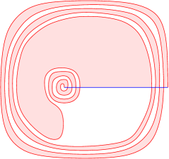
Figure 20: A lune of large area.

Proposition 9.8.

Define a relation $\prec$ on $\alpha\cap\beta$ by $x\prec y$ if and only if there is a sequence $x=x_{0},x_{1},\dots,x_{n}=y$ in $\alpha\cap\beta$ such that, for each $i$, there is a lune from $x_{i}$ to $x_{i-1}$ (see Figure 21). Then $\prec$ is a strict partial order.

Proof.

Since there is an $(\alpha,\beta)$-lune from $x_{i}$ to $x_{i-1}$ we have ${\mathcal{A}}(x_{i-1})<{\mathcal{A}}(x_{i})$ for every $i$ and hence, by induction, ${\mathcal{A}}(x_{0})<{\mathcal{A}}(x_{k})$. ∎

Figure 21: Lunes from $x_{i}$ to $x_{i-1}$.

Remark 9.9 (Mod Two Grading).

The endpoints of a lune have opposite intersection indices. Thus we may choose a ${\mathbb{Z}}/2{\mathbb{Z}}$-grading of ${\mathrm{CF}}(\alpha,\beta)$ by first choosing orientations of $\alpha$ and $\beta$ and then defining ${\mathrm{CF}}_{0}(\alpha,\beta)$ to be generated by the intersection points with intersection index $+1$ and ${\mathrm{CF}}_{1}(\alpha,\beta)$ to be generated by the intersection points with intersection index $-1$. Then the boundary operator interchanges these two subspaces and we have

$${\mathrm{alg}\left(\alpha,\beta\right)}=\dim{\mathrm{HF}}_{0}(\alpha,\beta)-\dim{\mathrm{HF}}_{1}(\alpha,\beta).$$

Remark 9.10 (Integer Grading).

Since each component of the path space ${\Omega}_{\alpha,\beta}$ is simply connected the ${\mathbb{Z}}/2{\mathbb{Z}}$-grading in Remark 9.9 can be refined to an integer grading. The grading is only well defined up to a global shift and the relative grading is given by the Viterbo–Maslov index. Then we obtain

$${\mathrm{alg}\left(\alpha,\beta\right)}=\chi({\mathrm{HF}}(\alpha,\beta))=\sum_{i\in{\mathbb{Z}}}(-1)^{i}\dim{\mathrm{HF}}_{i}(\alpha,\beta).$$

Figure 21 shows that there is no upper or lower bound on the relative index in the combinatorial Floer chain complex. Figure 22 shows that there is no upper bound on the dimension of ${\mathrm{CF}}_{i}(\alpha,\beta)$.

In the case of the $2$-torus $\Sigma={\mathbb{T}}^{2}={\mathbb{R}}^{2}/{\mathbb{Z}}^{2}$ the shift in the integer grading can be fixed using Seidel’s notion of a graded Lagrangian submanifold [33]. Namely, the tangent bundle of ${\mathbb{T}}^{2}$ is trivial so that each tangent space is equipped with a canonical isomorphism to ${\mathbb{R}}^{2}$. Hence every embedded circle $\alpha\subset{\mathbb{T}}^{2}$ determines a map $\alpha\to{\mathbb{R}\mathrm{P}}^{1}:z\mapsto T_{z}\alpha$. A grading of $\alpha$ is a lift of this map to the universal cover of ${\mathbb{R}\mathrm{P}}^{1}$. A choice of gradings for $\alpha$ and $\beta$ can be used to fix an integer grading of the combinatorial Floer homology.

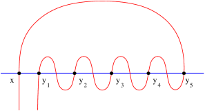
Figure 22: Lunes from $x$ to $y_{i}$.

Remark 9.11 (Integer Coefficients).

One can define combinatorial Floer homology with integer coefficients as follows. Fix an orientation of $\alpha$. Then each $(\alpha,\beta)$-lune $u:{\mathbb{D}}\to\Sigma$ comes with a sign

$$\nu(u):=\left\{\begin{array}[]{ll}+1,&\mbox{if the arc }u|_{{\mathbb{D}}\cap{\mathbb{R}}}:{\mathbb{D}}\cap{\mathbb{R}}\to\alpha\mbox{ is orientation preserving},\\ -1,&\mbox{if the arc }u|_{{\mathbb{D}}\cap{\mathbb{R}}}:{\mathbb{D}}\cap{\mathbb{R}}\to\alpha\mbox{ is orientation reversing}.\end{array}\right.$$

Now define the chain complex by

$${\mathrm{CF}}(\alpha,\beta;{\mathbb{Z}})=\bigoplus_{x\in\alpha\cap\beta}{\mathbb{Z}}x,$$

and

$${\partial}x:=\sum_{y\in\alpha\cap\beta}n(x,y;{\mathbb{Z}})y,\qquad n(x,y;{\mathbb{Z}}):=\sum_{[u]}\nu(u),$$

where the sum runs over all equivalence classes $[u]$ of smooth $(\alpha,\beta)$-lunes from $x$ to $y$. The results of Section 10 show that Theorem 9.1 remains valid with this refinement, and the results of Section 11 show that Theorem 9.2 also remains valid. We will not discuss here any orientation issue for the analytic Floer theory and leave it to others to investigate the validity of Theorem 9.3 with integer coefficients.

10 Hearts

Definition 10.1.

Let $x,z\in\alpha\cap\beta$. A broken $(\alpha,\beta)$-heart from $x$ to $z$ is a triple

$$h=(u,y,v)$$

such that $y\in\alpha\cap\beta$, $u$ is a smooth $(\alpha,\beta)$-lune from $x$ to $y$, and $v$ is a smooth $(\alpha,\beta)$-lune from $y$ to $z$. The point $y$ is called the midpoint of the heart. By Theorem 6.8 the broken $(\alpha,\beta)$-heart $h$ is uniquely determined by the septuple

$$\Lambda_{h}:=(x,y,z,u({\mathbb{D}}\cap{\mathbb{R}}),v({\mathbb{D}}\cap{\mathbb{R}}),u({\mathbb{D}}\cap S^{1}),v({\mathbb{D}}\cap S^{1})).$$

Two broken $(\alpha,\beta)$-hearts $h=(u,y,z)$ and $h^{\prime}=(u^{\prime},y^{\prime},z^{\prime})$ from $x$ to $z$ are called equivalent if $y^{\prime}=y$, $u^{\prime}$ is equivalent to $u$, and $v^{\prime}$ is equivalent to $v$. The equivalence class of $h$ is denoted by $[h]=([u],y,[v])$. The set of equivalence classes of broken $(\alpha,\beta)$-hearts from $x$ to $z$ will be denoted by ${\mathcal{H}}(x,z)$.

Proposition 10.2.

Let $h=(u,y,v)$ be a broken $(\alpha,\beta)$-heart from $x$ to $z$ and write $\Lambda_{h}=:(x,y,z,A_{xy},A_{yz},B_{xy},B_{yz}).$ Then exactly one of the following four alternatives (see Figure 23) holds:

$$\begin{split}{\bf(a)}\;A_{xy}\cap A_{yz}=\{y\},\;B_{yz}\subsetneq B_{xy}.\quad&{\bf(b)}\;A_{xy}\cap A_{yz}=\{y\},\;B_{xy}\subsetneq B_{yz}.\\ {\bf(c)}\;B_{xy}\cap B_{yz}=\{y\},\;A_{yz}\subsetneq A_{xy}.\quad&{\bf(d)}\;B_{xy}\cap B_{yz}=\{y\},\;A_{xy}\subsetneq A_{yz}.\end{split}$$

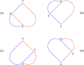
Figure 23: Four broken hearts.

Proof.

The combinatorial $(\alpha,\beta)$-lunes $\Lambda_{xy}:=\Lambda_{u}$ and $\Lambda_{yz}:=\Lambda_{v}$ have boundaries

$${\partial}\Lambda_{xy}=(x,y,A_{xy},B_{xy}),\qquad{\partial}\Lambda_{yz}=(y,z,A_{yz},B_{yz})$$

and their catenation $\Lambda_{xz}:=\Lambda_{xy}\#\Lambda_{yz}=(x,z,{\rm w}_{xy}+{\rm w}_{yz})$ has Viterbo–Maslov index two, by (38). Hence $m_{x}(\Lambda_{xy})+m_{x}(\Lambda_{yz})+m_{z}(\Lambda_{xy})+m_{z}(\Lambda_{yz})=4$, by the trace formula (37). Since $m_{x}(\Lambda_{xy})=m_{z}(\Lambda_{yz})=1$ this implies

$$m_{x}(\Lambda_{yz})+m_{z}(\Lambda_{xy})=2.$$ (46)

By Proposition 9.8 we have $x\neq z$. Hence $x$ cannot be an endpoint of $\Lambda_{yz}$. Thus $m_{x}(\Lambda_{yz})\geq 2$ whenever $x\in A_{yz}\cup B_{yz}$ and $m_{x}(\Lambda_{yz})\geq 4$ whenever $x\in A_{yz}\cap B_{yz}$. The same holds for $m_{z}(\Lambda_{xy})$. Hence it follows from (46) that $\Lambda_{xy}$ and $\Lambda_{yz}$ satisfy precisely one of the following conditions.

$$\begin{split}\mbox{\bf(a)}\;x\notin A_{yz}\cup B_{yz},\;z\in B_{xy}\setminus A_{xy}.\quad&\mbox{\bf(b)}\;x\in B_{yz}\setminus A_{yz},\;z\notin A_{xy}\cup B_{xy}.\\ \mbox{\bf(c)}\;x\notin A_{yz}\cup B_{yz},\;z\in A_{xy}\setminus B_{xy}.\quad&\mbox{\bf(d)}\;x\in A_{yz}\setminus B_{yz},\;z\notin A_{xy}\cup B_{xy}.\end{split}$$

This proves Proposition 10.2. ∎

Let $N\subset{\mathbb{C}}$ be an embedded convex half disc such that

$$[0,1]\cup{\mathbf{i}}[0,{\varepsilon})\cup(1+{\mathbf{i}}[0,{\varepsilon}))\subset{\partial}N,\qquad N\subset[0,1]+{\mathbf{i}}[0,1]$$

for some ${\varepsilon}>0$ and define

$$H:=([0,1]+{\mathbf{i}}[0,1])\cup({\mathbf{i}}+N)\cup(1+{\mathbf{i}}-{\mathbf{i}}N).$$

(See Figure 24.) The boundary of $H$ decomposes as

$${\partial}H={\partial}_{0}H\cup{\partial}_{1}H$$

where ${\partial}_{0}H$ denotes the boundary arc from $0$ to $1+{\mathbf{i}}$ that contains the horizontal interval $[0,1]$ and ${\partial}_{1}H$ denotes the arc from $0$ to $1+{\mathbf{i}}$ that contains the vertical interval ${\mathbf{i}}[0,1]$.

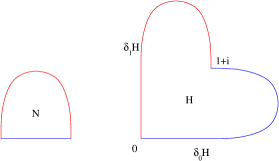
Figure 24: The domains $N$ and $H$.

Definition 10.3.

Let $x,z\in\alpha\cap\beta$. A smooth $(\alpha,\beta)$-heart of type (ac) from $x$ to $z$ is an orientation preserving immersion $w:H\to\Sigma$ that satisfies

$$w(0)=x,\qquad w(1+{\mathbf{i}})=z,\qquad w({\partial}_{0}H)\subsetneq\alpha,\qquad w({\partial}_{1}H)\subsetneq\beta.$$

Two smooth $(\alpha,\beta)$-hearts $w,w^{\prime}:H\to\Sigma$ are called equivalent iff there exists an orientation preserving diffeomorphism $\chi:H\to H$ such that

$$\chi(0)=0,\qquad\chi(1+{\mathbf{i}})=1+{\mathbf{i}},\qquad w^{\prime}=w\circ\chi.$$

A smooth $(\alpha,\beta)$-heart of type (bd) from $x$ to $z$ is a smooth $(\beta,\alpha)$-heart of type (ac) from $z$ to $x$. Let $w$ be a smooth $(\alpha,\beta)$-heart of type (ac) from $x$ to $y$ and $h=(u,y,v)$ be a broken $(\alpha,\beta)$-heart from $x$ to $y$ of type (a) or (c). The broken heart $h$ is called compatible with the smooth heart $w$ if there exist orientation preserving embeddings ${\varphi}:{\mathbb{D}}\to H$ and $\psi:{\mathbb{D}}\to H$ such that

$${\varphi}(-1)=0,\qquad\psi(1)=1+{\mathbf{i}},$$ (47)

$$H={\varphi}({\mathbb{D}})\cup\psi({\mathbb{D}}),\qquad{\varphi}({\mathbb{D}})\cap\psi({\mathbb{D}})={\varphi}({\partial}{\mathbb{D}})\cap\psi({\partial}{\mathbb{D}}),$$ (48)

$$u=w\circ{\varphi},\qquad v=w\circ\psi.$$ (49)

Lemma 10.4.

Let $h=(u,y,v)$ be a broken $(\alpha,\beta)$-heart of type (a), write

$$\Lambda_{h}=:(x,y,z,A_{xy},A_{yz},B_{xy},B_{yz}),$$

and define $A_{xz}$ and $B_{xz}$ by

$$A_{xz}:=A_{xy}\cup A_{yz},\qquad B_{xy}=:B_{xz}\cup B_{yz},\qquad B_{xz}\cap B_{yz}=\{z\}.$$

Let $w$ be a smooth $(\alpha,\beta)$-heart of type (ac) from $x$ to $z$ that is compatible with $h$ and let ${\varphi},\psi:{\mathbb{D}}\to H$ be embeddings that satisfy (47), (48), and (49). Then

$${\varphi}(e^{{\mathbf{i}}\theta_{1}})=1+{\mathbf{i}},$$ (50)

where $\theta_{1}\in[0,\pi]$ is defined by $u(e^{{\mathbf{i}}\theta_{1}})=z$, and

$${\varphi}({\mathbb{D}})\cap\psi({\mathbb{D}})=\psi({\mathbb{D}}\cap S^{1}),$$ (51)

$$w({\partial}_{0}H)=A_{xz},\qquad w({\partial}_{1}H)=B_{xz}.$$ (52)

Proof.

By definition of a smooth heart of type (ac), $w({\partial}_{0}H)$ is arc in $\alpha$ connecting $x$ to $z$ and $w({\partial}_{1}H)$ is an arc in $\beta$ connecting $x$ to $z$. Moreover, by (49),

$${\varphi}({\mathbb{D}}\cap{\mathbb{R}})\cup\psi({\mathbb{D}}\cap{\mathbb{R}})\subset w^{-1}(\alpha),\qquad{\varphi}({\mathbb{D}}\cap S^{1})\cup\psi({\mathbb{D}}\cap S^{1})\subset w^{-1}(\beta).$$

Now $w^{-1}(\alpha)$ is a union of disjoint embedded arcs, and so is $w^{-1}(\beta)$. One of the arcs in $w^{-1}(\alpha)$ contains ${\partial}_{0}H$ and one of the arcs in $w^{-1}(\beta)$ contains ${\partial}_{1}H$. Since ${\varphi}(-1)=0\in{\partial}_{0}H$ and the arc

$$w\circ{\varphi}({\mathbb{D}}\cap{\mathbb{R}})=u({\mathbb{D}}\cap{\mathbb{R}})=A_{xy}$$

does not contain $z$ we have

$${\varphi}({\mathbb{D}}\cap{\mathbb{R}})\subset{\partial}_{0}H,\qquad A_{xy}\subset w({\partial}_{0}H).$$

This implies the first equation in (52). Since $w\circ{\varphi}({\mathbb{D}}\cap S^{1})=u({\mathbb{D}}\cap S^{1})=B_{xy}$ is an arc containing $z$ we have

$${\partial}_{1}H\subset{\varphi}({\mathbb{D}}\cap S^{1}),\qquad w({\partial}_{1}H)\subset B_{xy}.$$

This implies the second equation in (52).

We prove (51). Choose $\theta_{1}\in[0,\pi]$ so that $u(e^{{\mathbf{i}}\theta_{1}})=z$ and denote

$$S_{0}:=\left\{e^{{\mathbf{i}}\theta}\,|\,0\leq\theta\leq\theta_{1}\right\},\qquad S_{1}:=\left\{e^{{\mathbf{i}}\theta}\,|\,\theta_{1}\leq\theta\leq\pi\right\},$$

So that

$${\mathbb{D}}\cap S^{1}=S_{0}\cup S_{1},\qquad u(S_{0})=B_{yz},\qquad u(S_{1})=B_{xz}.$$

Hence $w\circ{\varphi}(S_{1})=u(S_{1})=B_{xz}=w({\partial}_{1}H)$ and $0\in{\varphi}(S_{1})\cap{\partial}_{1}H$. Since $w$ is an immersion it follows that

$${\varphi}(S_{1})={\partial}_{1}H,\qquad{\varphi}(e^{{\mathbf{i}}\theta_{1}})=1+{\mathbf{i}}=\psi(1).$$

This proves (50). Moreover, by (49),

$$w\circ{\varphi}(S_{0})=u(S_{0})=B_{yz}=v({\mathbb{D}}\cap S^{1})=w\circ\psi({\mathbb{D}}\cap S^{1})$$

and $1+{\mathbf{i}}$ is an endpoint of both arcs ${\varphi}(S_{0})$ and $\psi({\mathbb{D}}\cap S^{1})$. Since $w$ is an immersion it follows that

$$\psi({\mathbb{D}}\cap S^{1})={\varphi}(S_{0})\subset{\varphi}({\mathbb{D}})\cap\psi({\mathbb{D}}).$$

To prove the converse inclusion, let $\zeta\in{\varphi}({\mathbb{D}})\cap\psi({\mathbb{D}})$. Then, by definition of a smooth heart, $\zeta\in{\varphi}({\partial}{\mathbb{D}})\cap\psi({\partial}{\mathbb{D}})$. If $\zeta\in{\varphi}({\mathbb{D}}\cap{\mathbb{R}})\cap\psi({\mathbb{D}}\cap{\mathbb{R}})$ then $w(\zeta)\in A_{xy}\cap A_{yz}=\{y\}$ and hence $\zeta=\psi(-1)\in\psi({\mathbb{D}}\cap S^{1})$. Now suppose $\zeta={\varphi}(e^{{\mathbf{i}}\theta})\in\psi({\mathbb{D}}\cap{\mathbb{R}})$ for some $\theta\in[0,\pi]$. Then we claim that $\theta\leq\theta_{1}$. To see this, consider the curve $\psi({\mathbb{D}}\cap{\mathbb{R}})$. By (49), this curve is mapped to $A_{yz}$ under $w$ and it contains the point $\psi(1)=1+{\mathbf{i}}$. Hence $\psi({\mathbb{D}}\cap{\mathbb{R}})\subset{\partial}_{0}H\setminus\{0\}$. But if $\theta>\theta_{1}$ then ${\varphi}(e^{{\mathbf{i}}\theta})\in{\partial}_{1}H\setminus\{1+{\mathbf{i}}\}$ and this set does not intersect ${\partial}_{0}H\setminus\{0\}$. Thus we have proved that $\theta\leq\theta_{1}$ and hence ${\varphi}(e^{{\mathbf{i}}\theta})\in{\varphi}(S_{0})=\psi({\mathbb{D}}\cap S^{1})$, as claimed. This proves Lemma 10.4. ∎

Proposition 10.5.

(i) Let $h=(u,y,v)$ be a broken $(\alpha,\beta)$-heart of type (a) or (c) from $x$ to $z$. Then there exists a smooth $(\alpha,\beta)$-heart $w$ of type (ac) from $x$ to $z$, unique up to equivalence, that is compatible with $h$.

(ii) Let $w$ be a smooth $(\alpha,\beta)$-heart of type (ac) from $x$ to $z$. Then there exists precisely one equivalence class of broken $(\alpha,\beta)$-hearts of type (a) from $x$ to $z$ that are compatible with $w$, and precisely one equivalence class of broken $(\alpha,\beta)$-hearts of type (c) from $x$ to $z$ that are compatible with $w$.

Proof.

We prove (i). Write

$$\Lambda_{h}=:(x,y,z,A_{xy},A_{yz},B_{xy},B_{yz})$$

and assume first that $\Lambda_{h}$ satisfies (a). We prove the existence of $[w]$. Choose a Riemannian metric on $\Sigma$ such that the direct sum decompositions

$$T_{y}\Sigma=T_{y}\alpha\oplus T_{y}\beta,\qquad T_{z}\Sigma=T_{z}\alpha\oplus T_{z}\beta$$

are orthogonal and $\alpha$ intersects small neighborhoods of $y$ and $z$ in geodesic arcs. Choose a diffeomorphism $\gamma:[0,1]\to B_{yz}$ such that $\gamma(0)=y$ and $\gamma(1)=z$ and let $\zeta(t)\in T_{\gamma(t)}\Sigma$ be a unit normal vector field pointing to the right. Then there are orientation preserving embeddings ${\varphi},\psi:{\mathbb{D}}\to H$ such that

$${\varphi}({\mathbb{D}})=([0,1]+{\mathbf{i}}[0,1])\cup({\mathbf{i}}+N),\qquad{\varphi}({\mathbb{D}}\cap{\mathbb{R}})=[0,1],$$

$$\psi({\mathbb{D}})=1+{\mathbf{i}}-{\mathbf{i}}N,\qquad\psi({\mathbb{D}}\cap S^{1})=1+{\mathbf{i}}[0,1],$$

and

$$u\circ{\varphi}^{-1}(1+s+{\mathbf{i}}t)=\exp_{\gamma(t)}(s\zeta(t))$$

for $0\leq t\leq 1$ and small $s\leq 0$, and

$$v\circ\psi^{-1}(1+s+{\mathbf{i}}t)=\exp_{\gamma(t)}(s\zeta(t))$$

for $0\leq t\leq 1$ and small $s\geq 0$. The function $w:H\to\Sigma$, defined by

$$w(z):=\left\{\begin{array}[]{rl}u\circ{\varphi}^{-1}(z),&\mbox{if }z\in{\varphi}({\mathbb{D}}),\\ v\circ\psi^{-1}(z),&\mbox{if }z\in\psi({\mathbb{D}}),\end{array}\right.$$

is a smooth $(\alpha,\beta)$-heart of type (ac) from $x$ to $z$ that is compatible with $h$.

We prove the uniqueness of $[w]$. Suppose that $w^{\prime}:H\to\Sigma$ is another smooth $(\alpha,\beta)$-heart of type (ac) that is compatible with $h$. Let ${\varphi}^{\prime}:{\mathbb{D}}\to H$ and $\psi^{\prime}:{\mathbb{D}}\to H$ be embeddings that satisfy (47) and (48) and suppose that $w^{\prime}$ is given by (49) with ${\varphi}$ and $\psi$ replaced by ${\varphi}^{\prime}$ and $\psi^{\prime}$. Then

$$w^{\prime}\circ{\varphi}^{\prime}\circ{\varphi}^{-1}(1+{\mathbf{i}}t) = u\circ{\varphi}^{-1}(1+{\mathbf{i}}t)$$

$$= v\circ\psi^{-1}(1+{\mathbf{i}}t)$$

$$= w^{\prime}\circ\psi^{\prime}\circ\psi^{-1}(1+{\mathbf{i}}t)$$

for $0\leq t\leq 1$ and, by (47) and (50),

$${\varphi}^{\prime}\circ{\varphi}^{-1}(1+{\mathbf{i}})=1+{\mathbf{i}}=\psi^{\prime}\circ\psi^{-1}(1+{\mathbf{i}}).$$

Since $w^{\prime}$ is an immersion it follows that

$${\varphi}^{\prime}\circ{\varphi}^{-1}(1+{\mathbf{i}}t)=\psi^{\prime}\circ\psi^{-1}(1+{\mathbf{i}}t)$$ (53)

for $0\leq t\leq 1$. Consider the map $\chi:H\to H$ given by

$$\chi(\zeta):=\left\{\begin{array}[]{rl}{\varphi}^{\prime}\circ{\varphi}^{-1}(\zeta),&\mbox{for }\zeta\in{\varphi}({\mathbb{D}}),\\ \psi^{\prime}\circ\psi^{-1}(\zeta),&\mbox{for }\zeta\in\psi({\mathbb{D}}).\end{array}\right.$$

By (53), this map is well defined. Since $H={\varphi}^{\prime}({\mathbb{D}})\cup\psi^{\prime}({\mathbb{D}})$, the map $\chi$ is surjective. We prove that $\chi$ is injective. Let $\zeta,\zeta^{\prime}\in H$ such that $\chi(\zeta)=\chi(\zeta^{\prime})$. If $\zeta,\zeta^{\prime}\in{\varphi}({\mathbb{D}})$ or $\zeta,\zeta^{\prime}\in\psi({\mathbb{D}})$ then it is obvious that $\zeta=\zeta^{\prime}$. Hence assume $\zeta\in{\varphi}({\mathbb{D}})$ and $\zeta^{\prime}\in\psi({\mathbb{D}})$. Then ${\varphi}^{\prime}\circ{\varphi}^{-1}(\zeta)=\psi^{\prime}\circ\psi^{-1}(\zeta^{\prime})$ and hence, by (51),

$$\psi^{\prime}\circ\psi^{-1}(\zeta^{\prime})\in\psi^{\prime}({\mathbb{D}}\cap S^{1}).$$

Hence $\zeta^{\prime}\in\psi({\mathbb{D}}\cap S^{1})\subset{\varphi}({\mathbb{D}})$, so $\zeta$ and $\zeta^{\prime}$ are both contained in ${\varphi}({\mathbb{D}})$, and it follows that $\zeta=\zeta^{\prime}$. Thus we have proved that $\chi:H\to H$ is a homeomorphism. Since $w^{\prime}=w\circ\chi$ it follows that $\chi$ is a diffeomorphism. This proves (i) in the case (a). The case (c) follows by reversing the orientation of $\Sigma$ and replacing $u$, $v$, $w$ by

$$u^{\prime}=u\circ\rho,\qquad v^{\prime}=v\circ\rho,\qquad w^{\prime}(\zeta)=w({\mathbf{i}}\bar{\zeta}),\qquad\rho(\zeta)=\frac{{\mathbf{i}}+\bar{\zeta}}{1+{\mathbf{i}}\bar{\zeta}}.$$

Thus $\rho:{\mathbb{D}}\to{\mathbb{D}}$ is an orientation reversing diffeomorphism with fixed points $\pm 1$ that interchanges ${\mathbb{D}}\cap{\mathbb{R}}$ and ${\mathbb{D}}\cap S^{1}$. The map $H\to H:\zeta\mapsto{\mathbf{i}}\bar{\zeta}$ is an orientation reversing diffeomorphism with fixed points $0$ and $1+{\mathbf{i}}$ that interchanges ${\partial}_{0}H$ and ${\partial}_{1}H$. This proves (i).

We prove (ii). Let $w:H\to\Sigma$ be a smooth $(\alpha,\beta)$-heart of type (ac) and denote

$$A_{xz}:=w({\partial}_{0}H),\qquad B_{xz}:=w({\partial}_{1}H).$$

Let $\gamma\subset w^{-1}(\beta)$ be the arc that starts at $1+{\mathbf{i}}$ and points into the interior of $H$. Let $\eta\in{\partial}H$ denote the second endpoint of $\gamma$. Since $\beta$ has no self-intersections we have $y:=w(\eta)\in A_{xz}.$ The arc $\gamma$ divides $H$ into two components, each of which is diffeomorphic to ${\mathbb{D}}$. (See Figure 25.)

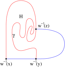
Figure 25: Breaking a heart.

The component which contains $0$ gives rise to a smooth $(\alpha,\beta)$-lune $u$ from $x$ to $y$ and the other component gives rise to a smooth $(\alpha,\beta)$-lune $v$ from $y$ to $z$. Let

$${\partial}\Lambda_{u}=:(x,y,A_{xy},B_{xy}),\qquad{\partial}\Lambda_{v}=:(y,z,A_{yz},B_{yz}).$$

Then

$$B_{xy}=B_{xz}\cup B_{yz},\qquad B_{yz}=w(\gamma).$$

By Theorem 6.5, $B_{xy}$ is an arc. Hence $B_{yz}\subsetneq B_{xy}$, and hence, by Proposition 10.2, the broken $(\alpha,\beta)$-heart $h=(u,y,v)$ from $x$ to $z$ satisfies (a). It is obviously compatible with $w$. A similar argument, using the arc $\gamma^{\prime}\subset w^{-1}(\alpha)$ that starts at $1+{\mathbf{i}}$ and points into the interior of $H$, proves the existence of a broken $(\alpha,\beta)$-heart $h^{\prime}\in{\mathcal{H}}(x,z)$ that satisfies (c) and is compatible with $w$. If ${\widetilde{h}}=({\widetilde{u}},{\widetilde{y}},{\widetilde{v}})$ is any other broken $(\alpha,\beta)$-heart of type (a) that is compatible with $w$, then it follows from uniqueness in part (i) that $w^{-1}({\widetilde{y}})=\eta$ is the endpoint of $\gamma$, hence ${\widetilde{y}}=y$, and hence, by Proposition 8.5, ${\widetilde{h}}$ is equivalent to $h$. This proves (ii) and Proposition 10.5. ∎

Proof of Theorem 9.1.

The square of the boundary operator is given by

$${\partial}{\partial}x=\sum_{z\in\alpha\cap\beta}n_{H}(x,z)z,$$

where

$$n_{H}(x,z):=\sum_{y\in\alpha\cap\beta}n(x,y)n(y,z)=\#{\mathcal{H}}(x,z).$$

By Proposition 10.5, and the analogous result for smooth $(\alpha,\beta)$-hearts of type (bd), there is an involution $\tau:{\mathcal{H}}(x,z)\to{\mathcal{H}}(x,z)$ without fixed points. Hence $n_{H}(x,z)$ is even for all $x$ and $z$ and hence ${\partial}\circ{\partial}=0$. This proves Theorem 9.1. ∎

11 Invariance under Isotopy

Proposition 11.1.

Let $x,y,x^{\prime},y^{\prime}\in\alpha\cap\beta$ be distinct intersection points such that

$$n(x,y)=n(x^{\prime},y)=n(x,y^{\prime})=1.$$

Let $u:{\mathbb{D}}\to\Sigma$ be a smooth $(\alpha,\beta)$-lune from $x$ to $y$ and assume that the boundary ${\partial}\Lambda_{u}=:(x,y,A,B)$ of its $(\alpha,\beta)$-trace satisfies

$$A\cap\beta=\alpha\cap B=\{x,y\}.$$

Then there is no smooth $(\alpha,\beta)$-lune from $x^{\prime}$ to $y^{\prime}$, i.e.

$$n(x^{\prime},y^{\prime})=0.$$

Moreover, extending the arc from $x$ to $y$ (in either $\alpha$ or $\beta$) beyond $y$, we encounter $x^{\prime}$ before $y^{\prime}$ (see Figures 26 and 27) and the two arcs $A^{\prime}\subset\alpha$ and $B^{\prime}\subset\beta$ from $x^{\prime}$ to $y^{\prime}$ that pass through $x$ and $y$ form an $(\alpha,\beta)$-trace that satisfies the arc condition.

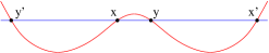
Figure 26: No lune from $x^{\prime}$ to $y^{\prime}$.

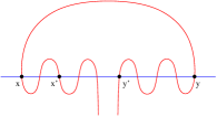
Figure 27: Lunes from $x$ or $x^{\prime}$ to $y$ or $y^{\prime}$.

Proof.

The proof has three steps.

Step 1. There exist $(\alpha,\beta)$-traces $\Lambda_{x^{\prime}y}=(x^{\prime},y,{\rm w}_{x^{\prime}y})$, $\Lambda_{yx}=(y,x,{\rm w}_{yx})$, and $\Lambda_{xy^{\prime}}=(x,y^{\prime},{\rm w}_{xy^{\prime}})$ with Viterbo–Maslov indices

$$\mu(\Lambda_{x^{\prime}y})=1,\qquad\mu(\Lambda_{yx})=-1,\qquad\mu(\Lambda_{xy^{\prime}})=1$$

such that

$${\rm w}_{x^{\prime}y}\geq 0,\qquad{\rm w}_{yx}\leq 0,\qquad{\rm w}_{x,y^{\prime}}\geq 0.$$

By hypothesis, there exist smooth $(\alpha,\beta)$-lunes from $x^{\prime}$ to $y$, from $x$ to $y$, and from $x$ to $y^{\prime}$. By Theorem 6.7 this implies the existence of combinatorial $(\alpha,\beta)$-lunes $\Lambda_{x^{\prime}y}=(x^{\prime},y,{\rm w}_{x^{\prime}y})$, $\Lambda_{xy}=(x,y,{\rm w}_{xy})$, and $\Lambda_{xy^{\prime}}=(x,y^{\prime},{\rm w}_{xy^{\prime}})$. To prove Step 1, reverse the direction of $\Lambda_{xy}$ to obtain the required $(\alpha,\beta)$-trace $\Lambda_{yx}=(y,x,{\rm w}_{yx})$ with ${\rm w}_{yx}:=-{\rm w}_{xy}$.

Step 2. Let $\Lambda_{x^{\prime}y}$, $\Lambda_{yx}$, $\Lambda_{xy^{\prime}}$ be as in Step 1. Then

$$\begin{split}m_{x^{\prime}}(\Lambda_{yx})=m_{y^{\prime}}(\Lambda_{yx})&=0,\\ m_{x}(\Lambda_{x^{\prime}y})=m_{y}(\Lambda_{xy^{\prime}})&=0,\\ m_{y^{\prime}}(\Lambda_{x^{\prime}y})=m_{x^{\prime}}(\Lambda_{xy^{\prime}})&=0.\end{split}$$ (54)

By hypothesis, the combinatorial $(\alpha,\beta)$-lune $\Lambda_{xy}=\Lambda_{u}$ has the boundary ${\partial}\Lambda_{xy}=(x,y,A,B)$ with $A\cap\beta=\alpha\cap B=\{x,y\}$. Hence ${\rm w}_{yx}=-{\rm w}_{xy}$ vanishes near every intersection point of $\alpha$ and $\beta$ other than $x$ and $y$. This proves the first equation in (54). By (38), the $(\alpha,\beta)$-trace $\Lambda_{x^{\prime}x}:=\Lambda_{x^{\prime}y}\#\Lambda_{yx}$ has Viterbo–Maslov index index zero. Hence, by the trace formula (37),

$$0 = m_{x^{\prime}}(\Lambda_{x^{\prime}x})+m_{x}(\Lambda_{x^{\prime}x})$$

$$= m_{x^{\prime}}(\Lambda_{x^{\prime}y})+m_{x^{\prime}}(\Lambda_{yx})+m_{x}(\Lambda_{x^{\prime}y})+m_{x}(\Lambda_{yx})$$

$$= m_{x}(\Lambda_{x^{\prime}y}).$$

Here the last equation follows from the fact that $m_{x^{\prime}}(\Lambda_{yx})=0$, $m_{x^{\prime}}(\Lambda_{x^{\prime}y})=1$, and $m_{x}(\Lambda_{yx})=-1$. The equation $m_{y}(\Lambda_{xy^{\prime}})=0$ is proved by an analogous argument, using the fact that $\Lambda_{yy^{\prime}}:=\Lambda_{yx}\#\Lambda_{xy^{\prime}}$ has Viterbo–Maslov index zero. This proves the second equation in (54). To prove the last equation in (54) we observe that the catenation

$$\Lambda_{x^{\prime}y^{\prime}}:=\Lambda_{x^{\prime}y}\#\Lambda_{yx}\#\Lambda_{xy^{\prime}}=\left(x^{\prime},y^{\prime},{\rm w}_{x^{\prime}y}+{\rm w}_{yx}+{\rm w}_{xy^{\prime}}\right)$$ (55)

has Viterbo–Maslov index one. Hence, by the trace formula (37),

$$2 = m_{x^{\prime}}(\Lambda_{x^{\prime}y^{\prime}})+m_{y^{\prime}}(\Lambda_{x^{\prime}y^{\prime}})$$

$$= m_{x^{\prime}}(\Lambda_{x^{\prime}y})+m_{x^{\prime}}(\Lambda_{yx})+m_{x^{\prime}}(\Lambda_{xy^{\prime}})$$

$$+\,m_{y^{\prime}}(\Lambda_{x^{\prime}y})+m_{y^{\prime}}(\Lambda_{yx})+m_{y^{\prime}}(\Lambda_{xy^{\prime}})$$

$$= 2+m_{x^{\prime}}(\Lambda_{xy^{\prime}})+m_{y^{\prime}}(\Lambda_{x^{\prime}y}).$$

Here the last equation follows from the first equation in (54) and the fact that $m_{x^{\prime}}(\Lambda_{x^{\prime}y})=m_{y^{\prime}}(\Lambda_{xy^{\prime}})=1$. Since the numbers $m_{x^{\prime}}(\Lambda_{xy^{\prime}})$ and $m_{y^{\prime}}(\Lambda_{x^{\prime}y})$ are nonnegative, this proves the last equation in (54). This proves Step 2.

Step 3. We prove the Proposition.

Let $\Lambda_{x^{\prime}y}$, $\Lambda_{yx}$, $\Lambda_{xy^{\prime}}$ be as in Step 1 and denote

$$\begin{split}{\partial}\Lambda_{x^{\prime}y}&=:(x^{\prime},y,A_{x^{\prime}y},B_{x^{\prime}y}),\\ {\partial}\Lambda_{yx}&=:(y,x,A_{yx},B_{yx}),\\ {\partial}\Lambda_{xy^{\prime}}&=:(x,y^{\prime},A_{xy^{\prime}},B_{xy^{\prime}}).\end{split}$$

By Step 2 we have

$$x,y^{\prime}\notin A_{x^{\prime}y}\cup B_{x^{\prime}y},\qquad x^{\prime},y^{\prime}\notin A_{yx}\cup B_{yx},\qquad x^{\prime},y\notin A_{xy^{\prime}}\cup B_{xy^{\prime}}.$$ (56)

In particular, the arc in $\alpha$ or $\beta$ from $y$ to $x^{\prime}$ contains neither $x$ nor $y^{\prime}$. Hence it is the extension of the arc from $x$ to $y$ and we encounter $x^{\prime}$ before $y^{\prime}$ as claimed. It follows also from (56) that the catenation $\Lambda_{x^{\prime}y^{\prime}}$ in (55) satisfies the arc condition and has boundary arcs

$$A_{x^{\prime}y^{\prime}}:=A_{x^{\prime}y}\cup A_{yx}\cup A_{xy^{\prime}},\qquad B_{x^{\prime}y^{\prime}}:=B_{x^{\prime}y}\cup B_{yx}\cup B_{xy^{\prime}}.$$

Thus $x\in A_{x^{\prime}y^{\prime}}$ and it follows from Step 2 that

$$m_{x}(\Lambda_{x^{\prime}y^{\prime}})=m_{x}(\Lambda_{x^{\prime}y})+m_{x}(\Lambda_{yx})+m_{x}(\Lambda_{xy^{\prime}})=0.$$

This shows that the function ${\rm w}_{x^{\prime}y^{\prime}}$ is not everywhere nonnegative, and hence $\Lambda_{x^{\prime}y^{\prime}}$ is not a combinatorial $(\alpha,\beta)$-lune. By Proposition 8.5 there is no other $(\alpha,\beta)$-trace with endpoints $x^{\prime},y^{\prime}$ that satisfies the arc condition. Hence $n(x^{\prime},y^{\prime})=0$. This proves Proposition 11.1 ∎

Proof of Theorem 9.2.

By composing with a suitable ambient isotopy assume without loss of generality that $\alpha=\alpha^{\prime}$. Furthermore assume the isotopy $\{\beta_{t}\}_{0\leq t\leq 1}$ with $\beta_{0}=\beta$ and $\beta_{1}=\beta^{\prime}$ is generic in the following sense. There exists a finite sequence of pairs $(t_{i},z_{i})\in[0,1]\times\Sigma$ such that

$$0<t_{1}<t_{2}<\cdots<t_{m}<1,$$

$\alpha\pitchfork_{z}\beta_{t}$ unless $(t,z)=(t_{i},z_{i})$ for some $i$, and for each $i$ there exists a coordinate chart $U_{i}\to{\mathbb{R}}^{2}:z\mapsto(\xi,\eta)$ at $z_{i}$ such that

$$\alpha\cap U_{i}=\left\{\eta=0\right\},\qquad\beta_{t}\cap U_{i}=\left\{\eta=-\xi^{2}\pm(t-t_{i})\right\}$$ (57)

for $t$ near $t_{i}$. It is enough to consider two cases.

Case 1 is $m=0$. In this case there exists an ambient isotopy ${\varphi}_{t}$ such that ${\varphi}_{t}(\alpha)=\alpha$ and ${\varphi}_{t}(\beta)=\beta_{t}$. It follows that the map ${\mathrm{CF}}(\alpha,\beta)\to{\mathrm{CF}}(\alpha,\beta^{\prime})$ induced by ${\varphi}_{1}:\alpha\cap\beta\to\alpha\cap\beta^{\prime}$ is a chain isomorphism that identifies the boundary maps.

In Case 2 we have $m=1$, the isotopy is supported near $U_{1}$, and (57) holds with the minus sign. Thus there are two intersection points in $U_{1}$ for $t<t_{1}$, no intersection points in $U_{1}$ for $t>t_{1}$, and all other intersection points of $\alpha$ and $\beta_{t}$ are independent of $t$. Denote by $x,y\in\alpha\cap\beta$ the intersection points that cancel at time $t=t_{1}$ and choose the ordering such that

$$n(x,y)=1.$$ (58)

Then $\alpha\cap\beta^{\prime}=(\alpha\cap\beta)\setminus\{x,y\}$. We prove in seven steps that

$$n^{\prime}(x^{\prime},y^{\prime})=n(x^{\prime},y^{\prime})+n(x^{\prime},y)n(x,y^{\prime})$$ (59)

for $x^{\prime},y^{\prime}\in\alpha\cap\beta^{\prime}$, where $n(x^{\prime},y^{\prime})$ denotes the number of $(\alpha,\beta)$-lunes from $x^{\prime}$ to $y^{\prime}$ and $n^{\prime}(x^{\prime},y^{\prime})$ denotes the number of $(\alpha,\beta^{\prime})$-lunes from $x^{\prime}$ to $y^{\prime}$.

Step 1. If there is no $(\alpha,\beta)$-trace from $x^{\prime}$ to $y^{\prime}$ that satisfies the arc condition then (59) holds.

In this case there is no $(\alpha,\beta_{t})$-trace from $x^{\prime}$ to $y^{\prime}$ that satisfies the arc condition for any $t$. Hence it follows from Theorem 6.5 that ${n(x^{\prime},y^{\prime})=n^{\prime}(x^{\prime},y^{\prime})=0}$ and it follows from Proposition 11.1 that $n(x^{\prime},y)n(x,y^{\prime})=0$. Hence (59) holds in this case.

Standing Assumptions, Part 1. From now on we assume that there is an $(\alpha,\beta)$-trace from $x^{\prime}$ to $y^{\prime}$ that satisfies the arc condition. Then there is an $(\alpha,\beta_{t})$-trace from $x^{\prime}$ to $y^{\prime}$ that satisfies the arc condition for every $t$. By Proposition 8.5, this $(\alpha,\beta_{t})$-trace is uniquely determined by $x^{\prime}$ and $y^{\prime}$. We denote it by $\Lambda_{x^{\prime}y^{\prime}}(t)$ and its boundary by

$${\partial}\Lambda_{x^{\prime}y^{\prime}}(t)=:(x^{\prime},y^{\prime},A_{x^{\prime}y^{\prime}},B_{x^{\prime}y^{\prime}}(t)).$$

Choose a universal covering $\pi:{\mathbb{C}}\to\Sigma$ so that ${\widetilde{\alpha}}={\mathbb{R}}$ is a lift of $\alpha$, the map ${\widetilde{z}}\mapsto{\widetilde{z}}+1$ is a covering transformation, and $\pi$ maps the interval $[0,1)$ bijectively onto $\alpha$. Let

$${\widetilde{\Lambda}}_{x^{\prime}y^{\prime}}(t)=({\widetilde{x}}^{\prime},{\widetilde{y}}^{\prime},{\rm w}_{{\widetilde{\Lambda}}_{x^{\prime}y^{\prime}}(t)})$$

be a continuous family of lifts of the $(\alpha,\beta_{t})$-traces to the universal cover $\pi:{\mathbb{C}}\to\Sigma$ with boundaries ${\partial}{\widetilde{\Lambda}}_{x^{\prime}y^{\prime}}(t)=({\widetilde{x}}^{\prime},{\widetilde{y}}^{\prime},{\widetilde{A}}_{x^{\prime}y^{\prime}},{\widetilde{B}}_{x^{\prime}y^{\prime}}(t))$.

Step 2. The lift ${\widetilde{\Lambda}}_{x^{\prime}y^{\prime}}(t)$ satisfies condition (II) (that the intersection index of ${\widetilde{A}}_{x^{\prime}y^{\prime}}$ and ${\widetilde{B}}_{x^{\prime}y^{\prime}}(t)$ at ${\widetilde{x}}^{\prime}$ is $+1$ and at ${\widetilde{y}}^{\prime}$ is $-1$) and condition (III) (that the winding numbers of ${\widetilde{A}}_{x^{\prime}y^{\prime}}-{\widetilde{B}}_{x^{\prime}y^{\prime}}(t)$ are zero or one near ${\widetilde{x}}^{\prime}$ and ${\widetilde{y}}^{\prime}$) either for all values of $t$ or for no value of $t$.

The intersection indices of ${\widetilde{A}}_{x^{\prime}y^{\prime}}$ and ${\widetilde{B}}_{x^{\prime}y^{\prime}}(t)$ at ${\widetilde{x}}^{\prime}$ and ${\widetilde{y}}^{\prime}$, and the winding numbers of ${\widetilde{A}}_{x^{\prime}y^{\prime}}-{\widetilde{B}}_{x^{\prime}y^{\prime}}(t)$ near ${\widetilde{x}}^{\prime}$ and ${\widetilde{y}}^{\prime}$, are obviously independent of $t$.

Step 3. If one of the arcs $A_{x^{\prime}y^{\prime}}(t)$ and $B_{x^{\prime}y^{\prime}}(t)$ does not pass through $U_{1}$ then (59) holds.

In this case the winding numbers do not change sign as $t$ varies and hence, by Step 2, $\nu(\Lambda_{x^{\prime}y^{\prime}}(t))$ is independent of $t$. Hence

$$n(x^{\prime},y^{\prime})=n^{\prime}(x^{\prime},y^{\prime}).$$

To prove equation (59) in this case, we must show that one of the numbers $n(x^{\prime},y)$ or $n(x,y^{\prime})$ vanishes. Suppose otherwise that

$$n(x^{\prime},y)=n(x,y^{\prime})=1.$$

Since $n(x,y)=1$, by equation (58), it follows from Proposition 11.1 that the two arcs from $x^{\prime}$ to $y^{\prime}$ that pass through $U_{1}$ form an $(\alpha,\beta)$-trace that satisfies the arc condition. Hence there are two $(\alpha,\beta)$-traces from $x^{\prime}$ to $y^{\prime}$ that satisfy the arc condition, which is impossible by Proposition 8.5. This contradiction proves Step 3.

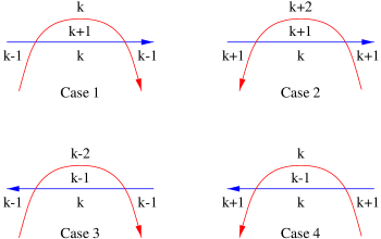
Figure 28: The winding numbers of ${\widetilde{\Lambda}}_{x^{\prime}y^{\prime}}$ in ${\widetilde{U}}_{1}$ for $t=0$.

Standing Assumptions, Part 2. From now on we assume that $A_{x^{\prime}y^{\prime}}$ and $B_{x^{\prime}y^{\prime}}(t)$ both pass through $U_{1}$. Denote by ${\widetilde{x}}$ and ${\widetilde{y}}$ the unique lifts of $x$ and $y$, respectively, in ${\widetilde{A}}_{x^{\prime}y^{\prime}}\cap{\widetilde{B}}_{x^{\prime}y^{\prime}}(0)$.

Under this assumption the winding number of ${\widetilde{\Lambda}}_{x^{\prime}y^{\prime}}(t)$ only changes in the area enclosed by the two arcs in the lift ${\widetilde{U}}_{1}$ of $U_{1}$ which contains ${\widetilde{x}}$ and ${\widetilde{y}}$. There are four cases, depending on the orientations of the two arcs from $x^{\prime}$ to $y^{\prime}$. (See Figure 28.) The next step deals with three of these cases.

Step 4. Assume that the orientation of $\alpha$ from $x^{\prime}$ to $y^{\prime}$ does not agree with one of the orientations from $x^{\prime}$ to $y$ or from $x$ to $y^{\prime}$, or else that this holds for $\beta$ (i.e. that one of the Cases 1,2,3 holds in Figure 28). Then (59) holds.

In Cases 1,2,3 the pattern of winding numbers shows (for any value of $k$) that ${\rm w}_{{\widetilde{\Lambda}}_{x^{\prime}y^{\prime}}(t)}$ is either nonnegative for all values of $t$ or is somewhere negative for all values of $t$. Hence, by Step 2, $\nu(\Lambda_{x^{\prime}y^{\prime}}(t))$ is independent of $t$, and hence $n(x^{\prime},y^{\prime})=n^{\prime}(x^{\prime},y^{\prime})$. Moreover, by Proposition 11.1, we have that in these cases $n(x,y^{\prime})n(x^{\prime},y)=0$. Hence (59) holds in the Cases 1,2,3.

Standing Assumptions, Part 3. From now on we assume that Case 4 holds in Figure 28, i.e. that the orientations of $\alpha$ and $\beta$ from $x^{\prime}$ to $y^{\prime}$ agree with the orientations from $x^{\prime}$ to $y$ and with the orientations from $x$ to $y^{\prime}$.

Step 5. Assume Case 4 and $n(x^{\prime},y)=n(x,y^{\prime})=1$. Then (59) holds.

By Proposition 11.1, we have $n(x^{\prime},y^{\prime})=0$. We must prove that $n^{\prime}(x^{\prime},y^{\prime})=1$. Let $\Lambda_{x^{\prime}y}$ and $\Lambda_{xy^{\prime}}$ be the $(\alpha,\beta)$-traces from $x^{\prime}$ to $y$, respectively from $x$ to $y^{\prime}$, that satisfy the arc condition and denote their lifts by ${\widetilde{\Lambda}}_{x^{\prime}y}$ and ${\widetilde{\Lambda}}_{xy^{\prime}}$. By (55),

$${\rm w}_{{\widetilde{\Lambda}}_{x^{\prime}y^{\prime}}(0)}({\widetilde{z}})={\rm w}_{{\widetilde{\Lambda}}_{x^{\prime}y}}({\widetilde{z}})+{\rm w}_{{\widetilde{\Lambda}}_{xy^{\prime}}}({\widetilde{z}})\qquad\mbox{for}\quad{\widetilde{z}}\in{\mathbb{C}}\setminus{\widetilde{U}}_{1}.$$ (60)

Thus ${\rm w}_{{\widetilde{\Lambda}}_{x^{\prime}y^{\prime}}(0)}\geq 0$ in ${\mathbb{C}}\setminus{\widetilde{U}}_{1}$. Moreover, by Theorem 6.7, the lifts ${\widetilde{\Lambda}}_{x^{\prime}y},{\widetilde{\Lambda}}_{xy^{\prime}}$ have winding numbers zero in the regions labelled by $k$ and $k-1$ in Figure 28, Case 4. Hence, by (60), we have $k=0$ and hence

$${\rm w}_{{\widetilde{\Lambda}}_{x^{\prime}y^{\prime}}(t)}\geq 0\qquad\mbox{for}\qquad t>t_{1}.$$

Thus we have proved that ${\widetilde{\Lambda}}_{x^{\prime}y^{\prime}}(t)$ satisfies (I) for $t>t_{1}$. Moreover, the Viterbo–Maslov index is given by

$$\mu({\widetilde{\Lambda}}_{x^{\prime}y^{\prime}}(t))=\mu({\widetilde{\Lambda}}_{x^{\prime}y})+\mu({\widetilde{\Lambda}}_{xy^{\prime}})-\mu({\widetilde{\Lambda}}_{xy})=1.$$

Hence, by Theorem 6.7, ${\widetilde{\Lambda}}_{x^{\prime}y^{\prime}}(t)$ is a combinatorial lune for $t>t_{1}$ and we have $n^{\prime}(x^{\prime},y^{\prime})=1$.

Step 6. Assume Case 4 and $n^{\prime}(x^{\prime},y^{\prime})=1$. Then (59) holds.

The winding numbers of ${\widetilde{\Lambda}}_{x^{\prime}y^{\prime}}(1)$ are nonnegative and hence we must have $k\geq 0$ in Figure 28, Case 4. If $k>0$ then the winding numbers of ${\widetilde{\Lambda}}_{x^{\prime}y^{\prime}}(0)$ are also nonnegative and hence, by Step 2, $n(x^{\prime},y^{\prime})=1$. Hence, by (58) and Proposition 11.1, one of the numbers $n(x^{\prime},y)$ and $n(x,y^{\prime})$ must vanish, and hence (59) holds when $k>0$.

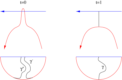
Figure 29: A lune splits.

Now assume $k=0$. Then $n(x^{\prime},y^{\prime})=0$ and we must prove that

$$n(x^{\prime},y)=n(x,y^{\prime})=1.$$

To see this, we choose a smooth $({\widetilde{\alpha}},{\widetilde{\beta}}^{\prime})$-lune

$${\widetilde{u}}^{\prime}:{\mathbb{D}}\to{\mathbb{C}}$$

from ${\widetilde{x}}^{\prime}$ to ${\widetilde{y}}^{\prime}$. Since $k=0$ this lune has precisely one preimage in the region in ${\widetilde{U}}_{1}$ where there winding number is $k+1=1\neq 0$ for $t=1$. Choose an embedded arc

$${\widetilde{\gamma}}:[0,1]\to{\mathbb{C}}$$

in ${\widetilde{U}}_{1}$ for $t=1$ connecting the two branches of ${\widetilde{\alpha}}$ and ${\widetilde{\beta}}^{\prime}$ such that ${\widetilde{\gamma}}$ intersects ${\widetilde{\alpha}}$ and ${\widetilde{\beta}}^{\prime}$ only at the endpoints (see Figure 29). Then

$$\gamma:={{{\widetilde{u}}^{\prime}\,}}^{-1}({\widetilde{\gamma}})$$

divides ${\mathbb{D}}$ into two components. Deform the curve ${\widetilde{\beta}}^{\prime}$ along ${\widetilde{\gamma}}$ to a curve ${\widetilde{\beta}}^{\prime\prime}$ that intersects ${\widetilde{\alpha}}$ in two points ${\widetilde{x}}^{\prime\prime},{\widetilde{y}}^{\prime\prime}\in{\widetilde{U}}_{1}$. The preimage of ${\widetilde{\beta}}^{\prime\prime}$ under ${\widetilde{u}}^{\prime}$ contains two arcs $\gamma^{-}$ and $\gamma^{+}$, parallel to $\gamma$, in the two components of ${\mathbb{D}}$. This results in two half-discs contained in ${\mathbb{D}}$, and the restriction of ${\widetilde{u}}$ to these two half discs gives rise to two $({\widetilde{\alpha}},{\widetilde{\beta}}^{\prime\prime})$-lunes, one from ${\widetilde{x}}^{\prime}$ to ${\widetilde{y}}^{\prime\prime}$ and one from ${\widetilde{x}}^{\prime\prime}$ to ${\widetilde{y}}^{\prime}$ (see Figure 29). Moreover ${\widetilde{\beta}}^{\prime\prime}$ descends to an embedded loop in $\Sigma$ that is isotopic to $\beta$ through loops that are transverse to $\alpha$. Hence $n(x^{\prime},y)=n(x,y^{\prime})=1$, as claimed.

Step 7. Assume Case 4 and $n^{\prime}(x^{\prime},y^{\prime})=n(x^{\prime},y)n(x,y^{\prime})=0$. Then (59) holds.

We must prove that $n(x^{\prime},y^{\prime})=0$. By Step 2, conditions (II) and (III) on ${\widetilde{\Lambda}}_{x^{\prime}y^{\prime}}(t)$ are independent of $t$ and so we have that $n(x^{\prime},y^{\prime})=0$ whenever these conditions are not satisfied. Hence assume that ${\widetilde{\Lambda}}_{x^{\prime}y^{\prime}}(t)$ satisfies (II) and (III) for every $t$. If $k>0$ in Figure 28 then condition (I) also holds for every $t$ and hence $n(x^{\prime},y^{\prime})=n^{\prime}(x^{\prime},y^{\prime})=1$, a contradiction. If $k\leq 0$ in Figure 28 then ${\widetilde{\Lambda}}_{x^{\prime}y^{\prime}}(0)$ does not satisfy (I) and hence $n(x^{\prime},y^{\prime})=0$, as claimed.

Thus we have established (59). Hence, by Lemma C.1, ${\mathrm{HF}}(\alpha,\beta)$ is isomorphic to ${\mathrm{HF}}(\alpha,\beta^{\prime})$. This proves Theorem 9.2. ∎

12 Lunes and Holomorphic Strips

We assume throughout that $\Sigma$ and $\alpha,\beta\subset\Sigma$ satisfy hypothesis (H). We also fix a complex structure $J$ on $\Sigma$. A holomorphic $(\alpha,\beta)$-strip is a holomorphic map $v:{\mathbb{S}}\to\Sigma$ of finite energy such that

$$v({\mathbb{R}})\subset\alpha,\qquad v({\mathbb{R}}+{\mathbf{i}})\subset\beta.$$ (61)

It follows [32, Theorem A] that the limits

$$x=\lim_{s\to-\infty}v(s+{\mathbf{i}}t),\qquad y=\lim_{s\to+\infty}v(s+{\mathbf{i}}t)$$ (62)

exist; the convergence is exponential and uniform in $t$; moreover ${\partial}_{s}v$ and all its derivatives converge exponentially to zero as $s$ tends to $\pm\infty$. Call two holomorphic strips equivalent if they differ by a time shift. Every holomorphic strip $v$ has a Viterbo–Maslov index $\mu(v)$, defined as follows. Trivialize the complex line bundle $v^{*}T\Sigma\to{\mathbb{S}}$ such that the trivialization converges to a frame of $T_{x}\Sigma$ as $s$ tends to $-\infty$ and to a frame of $T_{y}\Sigma$ as $s$ tends to $+\infty$ (with convergence uniform in $t$). Then $s\mapsto T_{v(s,0)}\alpha$ and $s\mapsto T_{v(s,1)}\beta$ are Lagrangian paths and their relative Maslov index is $\mu(v)$ (see [39] and [30]).

At this point it is convenient to introduce the notation

$${\mathcal{M}}^{\mathrm{Floer}}(x,y;J):=\frac{\left\{v:{\mathbb{S}}\to\Sigma\,\bigg{|}\,\begin{array}[]{l}v\mbox{ is a holomorphic $(\alpha,\beta)$-strip}\\ \mbox{from $x$ to $y$ with $\mu(v)=1$}\end{array}\right\}}{\mbox{time shift}}$$

for the moduli space of index one holomorphic strips from $x$ to $y$ up to time shift. This moduli space depends on the choice of a complex structure $J$ on $\Sigma$. We also introduce the notation

$${\mathcal{M}}^{\mathrm{comb}}(x,y):=\frac{\left\{u:{\mathbb{D}}\to\Sigma\,\bigg{|}\,\begin{array}[]{l}u\mbox{ is a smooth $(\alpha,\beta)$-lune}\\ \mbox{from $x$ to $y$}\end{array}\right\}}{\mbox{isotopy}}$$

for the moduli space of (equivalence classes of) smooth $(\alpha,\beta)$-lunes. This space is independent of the choice of $J$. We show that there is a bijection between these moduli spaces for every pair $x,y\in\alpha\cap\beta$.

Given a smooth $(\alpha,\beta)$-lune $u:{\mathbb{D}}\to\Sigma$, the Riemann mapping theorem gives a unique homeomorphism ${\varphi}_{u}:{\mathbb{D}}\to{\mathbb{D}}$ such that the restriction of ${\varphi}_{u}$ to ${\mathbb{D}}\setminus\{\pm 1\}$ is a diffeomorphism and

$${\varphi}_{u}(-1)=-1,\qquad{\varphi}_{u}(0)=0,\qquad{\varphi}_{u}(1)=1,\qquad{\varphi}_{u}^{*}u^{*}J={\mathbf{i}}.$$ (63)

Let $g:{\mathbb{S}}\to{\mathbb{D}}\setminus\{\pm 1\}$ be the holomorphic diffeomorphism given by

$$g(s+{\mathbf{i}}t):=\frac{e^{(s+{\mathbf{i}}t)\pi/2}-1}{e^{(s+{\mathbf{i}}t)\pi/2}+1}.$$ (64)

Then, for every $(\alpha,\beta)$-lune $u$, the composition $v:=u\circ{\varphi}_{u}\circ g$ is a holomorphic $(\alpha,\beta)$-strip.

Theorem 12.1.

Assume (H), let $x,y\in\alpha\cap\beta$, and choose a complex structure $J$ on $\Sigma$. Then the map $u\mapsto u\circ{\varphi}_{u}\circ g$ induces a bijection

$${\mathcal{M}}^{\mathrm{comb}}(x,y)\to{\mathcal{M}}^{\mathrm{Floer}}(x,y;J):[u]\mapsto[u\circ{\varphi}_{u}\circ g]$$ (65)

between the corresponding moduli spaces.

Proof.

See page 12 below. ∎

The proof of Theorem 12.1 relies on the asymptotic analysis of holomorphic strips in [32] (see Appendx D for a summary) and on an explicit formula for the Viterbo–Maslov index. For each intersection point $x\in\alpha\cap\beta$ we denote by $\theta_{x}\in(0,\pi)$ the angle from $T_{x}\alpha$ to $T_{x}\beta$ with respect to our complex structure $J$. Thus

$$T_{x}\beta=\left(\cos(\theta_{x})+\sin(\theta_{x})J\right)T_{x}\alpha,\qquad 0<\theta_{x}<\pi.$$ (66)

Fix a nonconstant holomorphic $(\alpha,\beta)$-strip $v:{\mathbb{S}}\to\Sigma$ from $x$ to $y$. Choose a holomorphic coordinate chart $\psi_{y}:U_{y}\to{\mathbb{C}}$ on an open neighborhood $U_{y}\subset\Sigma$ of $y$ such that $\psi_{y}(y)=0$. By [32, Theorem C] (see also Corollary D.2) there is a complex number $c_{y}$ and a integer $\nu_{y}(v)\geq 1$ such that

$$\psi_{y}(v(s+{\mathbf{i}}t))=c_{y}e^{-(\nu_{y}(v)\pi-\theta_{y})(s+{\mathbf{i}}t)}+O(e^{-(\nu_{y}(v)\pi-\theta_{y}+\delta)s})$$ (67)

for some $\delta>0$ and all $s>0$ sufficiently close to $+\infty$. The complex number $c_{y}$ belongs to the tangent space $T_{0}(\psi_{y}(\alpha\cap U_{y}))$ and the integer $\nu_{y}(v)$ is independent of the choice of the coordinate chart.

Now let us interchange $\alpha$ and $\beta$ as well as $x$ and $y$, and replace $v$ by the $(\beta,\alpha)$-holomorphic strip

$$s+{\mathbf{i}}t\mapsto v(-s+{\mathbf{i}}(1-t))$$

from $y$ to $x$. Choose a holomorphic coordinate chart $\psi_{x}:U_{x}\to{\mathbb{C}}$ on an open neighborhood $U_{x}\subset\Sigma$ of $x$ such that $\psi_{x}(x)=0$. Using [32, Theorem C] again we find that there is a complex number $c_{x}$ and an integer $\nu_{x}(v)\geq 0$ such that

$$\psi_{x}(v(s+{\mathbf{i}}t))=c_{x}e^{(\nu_{x}(v)\pi+\theta_{x})(s+{\mathbf{i}}t)}+O(e^{(\nu_{x}(v)\pi+\theta_{x}+\delta)s})$$ (68)

for some $\delta>0$ and all $s<0$ sufficiently close to $-\infty$. As before, the complex number $c_{x}$ belongs to the tangent space $T_{0}(\psi_{x}(\alpha\cap U_{x}))$ and the integer $\nu_{x}(v)$ is independent of the choice of the coordinate chart.

Denote the set of critical points of $v$ by

$$C_{v}:=\left\{z\in{\mathbb{S}}\,|\,dv(z)=0\right\}.$$

It follows from Corollary D.2 (i) that this is a finite set. For $z\in C_{v}$ denote by $\nu_{z}(v)\in{\mathbb{N}}$ the order to which $dv$ vanishes at $z$. Thus the first nonzero term in the Taylor expansion of $v$ at $z$ (in a local holomorphic coordinate chart on $\Sigma$ centered at $v(z)$) has order $\nu_{z}(v)+1$.

Theorem 12.2.

Assume (H) and choose a complex structure $J$ on $\Sigma$. Let $x,y\in\alpha\cap\beta$ and $v:{\mathbb{S}}\to\Sigma$ be a nonconstant holomorphic $(\alpha,\beta)$-strip from $x$ to $y$. Then the linearized operator $D_{v}$ associated to this strip in Floer theory is surjective. Moreover, the Viterbo–Maslov index of $v$ is equal to the Fredholm index of $D_{v}$ and is given by the index formula

$$\mu(v)=\nu_{x}(v)+\nu_{y}(v)+\sum_{z\in C_{v}\cap{\partial}{\mathbb{S}}}\nu_{z}(v)+2\sum_{z\in C_{v}\cap{\rm int}({\mathbb{S}})}\nu_{z}(v).$$ (69)

The right hand side in equation (69) is positive because all summands are nonnegative and ${\nu_{y}(v)\geq 1}$.

Proof.

See page 12 below. ∎

The surjectivity statement in Theorem 12.2 has been observed by many authors. A proof for holomorphic polygons is contained in Seidel’s book [34].

We will need a more general index formula (equation (76) below) which we explain next. Choose a Riemannian metric on $\Sigma$ that is compatible with the complex structure $J$. This metric induces a Hermitian structure on the pullback tangent bundle $v^{*}T\Sigma\to{\mathbb{S}}$ and the Hilbert spaces $W^{1,2}({\mathbb{S}},v^{*}T\Sigma)$ and $L^{2}({\mathbb{S}},v^{*}T\Sigma)$ are understood with respect to this induced structure. These Hilbert spaces are independent of the choice of the metric on $\Sigma$, only their inner products depend on this choice. The linearized operator

$$D_{v}:W_{\mathrm{BC}}^{1,2}({\mathbb{S}},v^{*}T\Sigma)\to L^{2}({\mathbb{S}},v^{*}T\Sigma)$$

with

$$W_{\mathrm{BC}}^{1,2}({\mathbb{S}},v^{*}T\Sigma):=\left\{\hat{v}\in W^{1,2}({\mathbb{S}},v^{*}T\Sigma)\,\bigg{|}\,\begin{array}[]{l}\hat{v}(s,0)\in T_{v(s,0)}\alpha\;\forall s\in{\mathbb{R}}\\ \hat{v}(s,1)\in T_{v(s,1)}\beta\;\forall s\in{\mathbb{R}}\end{array}\right\}$$

is given by

$$D_{v}\hat{v}=\nabla\kern-2.15277pt{}_{s}\hat{v}+J\nabla\kern-2.15277pt{}_{t}\hat{v}$$

for $\hat{v}\in W^{1,2}_{\mathrm{BC}}({\mathbb{S}},v^{*}T\Sigma)$, where $\nabla$ denotes the Levi-Civita connection. Here we use the fact that $\nabla J=0$ because $J$ is integrable. We remark that, first, this is a Fredholm operator for every smooth map $v:{\mathbb{S}}\to\Sigma$ satisfying (61) and (62) (where the convergence is exponential and uniformly in $t$, and ${\partial}_{s}v$, $\nabla\kern-2.15277pt{}_{s}{\partial}_{s}v$, $\nabla\kern-2.15277pt{}_{s}{\partial}_{t}v$ converge exponentially to zero as $s$ tends to $\pm\infty$). Second, the definition of the Viterbo–Maslov index $\mu(v)$ extends to this setting and it is equal to the Fredholm index of $D_{v}$ (see [31]) Third, the operator $D_{v}$ is independent of the choice of the Riemannian metric whenever $v$ is an $(\alpha,\beta)$-holomorphic strip.

Next we choose a unitary trivialization

$$\Phi(s,t):{\mathbb{C}}\to T_{v(s,t)}\Sigma$$

of the pullback tangent bundle such that

$$\Phi(s,0){\mathbb{R}}=T_{v(s,0)}\alpha,\qquad\Phi(s,1){\mathbb{R}}=T_{v(s,1)}\beta,$$

and $\Phi(s,t)=\Psi_{t}(v(s,t))$ for $\mathopen{|}s\mathclose{|}$ sufficiently large. Here $\Psi_{t}$, $0\leq t\leq 1$, is a smooth family of unitary trivializations of the tangent bundle over a neighborhood $U_{x}\subset\Sigma$ of $x$, respectively $U_{y}\subset\Sigma$ of $y$, such that $\Psi_{0}(z){\mathbb{R}}=T_{z}\alpha$ for $z\in(U_{x}\cup U_{y})\cap\alpha$ and $\Psi_{1}(z){\mathbb{R}}=T_{z}\beta$ for $z\in(U_{x}\cup U_{y})\cap\beta$. Then

$$\begin{split}{\mathcal{W}}&:=\Phi^{-1}W^{1,2}_{\mathrm{BC}}({\mathbb{S}},v^{*}T\Sigma)=\left\{\xi\in W^{1,2}({\mathbb{S}},{\mathbb{C}})\,|\,\xi(s,0),\xi(s,1)\in{\mathbb{R}}\;\forall s\in{\mathbb{R}}\right\},\\ {\mathcal{H}}&:=\Phi^{-1}L^{2}({\mathbb{S}},v^{*}T\Sigma)=L^{2}({\mathbb{S}},{\mathbb{C}}).\end{split}$$

The operator $D_{S}:=\Phi^{-1}\circ D_{v}\circ\Phi:{\mathcal{W}}\to{\mathcal{H}}$ has the form

$$D_{S}\xi={\partial}_{s}\xi+{\mathbf{i}}{\partial}_{t}\xi+S\xi$$ (70)

where the function $S:{\mathbb{S}}\to{\rm End}_{\mathbb{R}}({\mathbb{C}})$ is given by

$$S(s,t):=\Phi(s,t)^{-1}\Bigl{(}\nabla\kern-2.15277pt{}_{s}\Phi(s,t)+J(v(s,t))\nabla\kern-2.15277pt{}_{t}\Phi(s,t)\Bigr{)}.$$

The matrix $\Phi^{-1}\nabla\kern-2.15277pt{}_{s}\Phi$ is skew-symmetric and the matrix $\Phi^{-1}J(v)\nabla\kern-2.15277pt{}_{t}\Phi$ is symmetric. Moreover, it follows from our hypotheses on $v$ and the trivialization that $S$ converges exponentially and $\Phi^{-1}\nabla\kern-2.15277pt{}_{s}\Phi$ as well as ${\partial}_{s}S$ converge exponentially to zero as as $s$ tends to $\pm\infty$. The limits of $S$ are the symmetric matrix functions

$$\begin{split}S_{x}(t)&:=\lim_{s\to-\infty}S(s,t)=\Psi_{t}(x)^{-1}J(x){\partial}_{t}\Psi_{t}(x),\\ S_{y}(t)&:=\lim_{s\to+\infty}S(s,t)=\Psi_{t}(y)^{-1}J(y){\partial}_{t}\Psi_{t}(y).\end{split}$$ (71)

Thus there exist positive constants $c$ and ${\varepsilon}$ such that

$$\begin{split}\left|S(s,t)-S_{x}(t)\right|+\left|{\partial}_{s}S(s,t)\right|&\leq ce^{{\varepsilon}s},\\ \left|S(s,t)-S_{y}(t)\right|+\left|{\partial}_{s}S(s,t)\right|&\leq ce^{-{\varepsilon}s}\end{split}$$ (72)

for every $s\in{\mathbb{R}}$. This shows that the operator (70) satisfies the hypotheses of [32, Lemma 3.6]. This lemma asserts the following. Let $\xi\in{\mathcal{W}}$ be a nonzero function in the kernel of $D_{S}$:

$$\xi\in{\mathcal{W}},\qquad D_{S}\xi={\partial}_{s}\xi+{\mathbf{i}}{\partial}_{t}\xi+S\xi=0,\qquad\xi\neq 0.$$

Then there exist nonzero functions $\xi_{x},\xi_{y}:[0,1]\to{\mathbb{C}}$ and positive real numbers $\lambda_{x},\lambda_{y},C,\delta$ such that

$$\begin{split}{\mathbf{i}}\dot{\xi}_{x}(t)+S_{x}(t)\xi_{x}(t)&=-\lambda_{x}\xi_{x}(t),\qquad\xi_{x}(0),\xi_{x}(1)\in{\mathbb{R}}\\ {\mathbf{i}}\dot{\xi}_{y}(t)+S_{y}(t)\xi_{y}(t)&=\lambda_{y}\xi_{y}(t),\qquad\xi_{y}(0),\xi_{y}(1)\in{\mathbb{R}}\end{split}$$ (73)

and

$$\begin{split}\left|\xi(s,t)-e^{\lambda_{x}s}\xi_{x}(t)\right|&\leq Ce^{(\lambda_{x}+\delta)s},\qquad s\leq 0\\ \left|\xi(s,t)-e^{-\lambda_{y}s}\xi_{y}(t)\right|&\leq Ce^{-(\lambda_{y}+\delta)s},\qquad s\geq 0.\end{split}$$ (74)

We prove that there exist integers $\iota(x,\xi)\geq 0$ and $\iota(y,\xi)\geq 1$ such that

$$\lambda_{x}=\iota(x,\xi)\pi+\theta_{x},\qquad\lambda_{y}=\iota(y,\xi)\pi-\theta_{y}.$$ (75)

Here $\theta_{x}$ is chosen as above such that

$$T_{x}\beta=\exp(\theta_{x}J(x))T_{x}\alpha,\qquad 0<\theta_{x}<\pi,$$

and the same for $\theta_{y}$. To prove (75), we observe that the function

$$v_{x}(t):=\Psi_{t}(x)\xi_{x}(t)$$

satisfies

$$J(x)\dot{v}_{x}(t)=-\lambda_{x}v_{x}(t),\qquad v_{x}(0)\in T_{x}\alpha,\qquad v_{x}(1)\in T_{x}\beta.$$

Hence $v_{x}(t)=\exp(t\lambda_{x}J(x))v_{x}(0)$ and this proves the first equation in (75). Likewise, the function $v_{y}(t):=\Psi_{t}(y)\xi_{y}(t)$ satisfies $J(y)\dot{v}_{y}(t)=\lambda_{y}v_{y}(t)$ and $v_{y}(0)\in T_{y}\alpha$ and $v_{y}(1)\in T_{y}\beta$. Hence $v_{y}(t)=\exp(-t\lambda_{y}J(y))v_{y}(0)$, and this proves the second equation in (75).

Lemma 12.3.

Suppose $S$ satisfies the asymptotic condition (72) and let $\xi\in{\mathcal{W}}$ be a smooth function with isolated zeros that satisfies (73), (74), and (75). Then the Fredholm index of $D_{S}$ is given by the linear index formula

$$\mathrm{index}(D_{S})=\iota(x,\xi)+\iota(y,\xi)+\sum_{z\in{\partial}{\mathbb{S}}\atop\xi(z)=0}\iota(z,\xi)+2\sum_{z\in{\rm int}({\mathbb{S}})\atop\xi(z)=0}\iota(z,\xi).$$ (76)

In the second sum $\iota(z,\xi)$ denotes the index of $z$ as a zero of $\xi$. In the first sum $\iota(z,\xi)$ denotes the degree of the loop $[0,\pi]\to{\mathbb{R}\mathrm{P}}^{1}:\theta\mapsto\xi(z+{\varepsilon}e^{{\mathbf{i}}\theta}){\mathbb{R}}$ when $z\in{\mathbb{R}}$ and of the loop $[0,\pi]\to{\mathbb{R}\mathrm{P}}^{1}:\theta\mapsto\xi(z-{\varepsilon}e^{{\mathbf{i}}\theta}){\mathbb{R}}$ when $z\in{\mathbb{R}}+{\mathbf{i}}$; in both cases ${\varepsilon}>0$ is chosen so small that the closed ${\varepsilon}$-neighborhood of $z$ contains no other zeros of $\xi$.

Proof.

Since $\xi_{x}$ and $\xi_{y}$ have no zeros, by (73), it follows from equation (74) that the zeros of $\xi$ are confined to a compact subset of ${\mathbb{S}}$. Moreover the zeros of $\xi$ are isolated and so the right hand side of (76) is a finite sum. Now let $\xi_{0}:{\mathbb{S}}\to{\mathbb{C}}$ be the unique solution of the equation

$${\mathbf{i}}{\partial}_{t}\xi_{0}(s,t)+S(s,t)\xi_{0}(s,t)=0,\qquad\xi_{0}(s,0)=1.$$ (77)

Then

$$\begin{split}\xi_{0,x}(t)&:=\lim_{s\to-\infty}\xi_{0}(s,t)=\Psi_{t}(x)^{-1}\Psi_{0}(x)1,\\ \xi_{0,y}(t)&:=\lim_{s\to+\infty}\xi_{0}(s,t)=\Psi_{t}(y)^{-1}\Psi_{0}(y)1.\end{split}$$ (78)

Thus the Lagrangian path

$${\mathbb{R}}\to{\mathbb{R}\mathrm{P}}^{1}:s\mapsto\Lambda_{S}(s):={\mathbb{R}}\xi(s,1)$$

is asymptotic to the subspace $\Psi_{1}(x)^{-1}T_{x}\alpha$ as $s$ tends to $-\infty$ and to the subspace $\Psi_{1}(y)^{-1}T_{y}\alpha$ as $s$ tends to $+\infty$. These subspaces are both transverse to ${\mathbb{R}}$. By the spectral-flow-equals-Maslov-index theorem in [31] the Fredholm index of $D_{S}$ is equal to the relative Maslov index of the pair $(\Lambda_{S},{\mathbb{R}})$:

$$\mathrm{index}(D_{S})=\mu(\Lambda_{S},{\mathbb{R}}).$$ (79)

It follows from (73) and (78) that

$$\frac{\xi_{0,x}(t)}{\xi_{x}(t)}=\frac{e^{-{\mathbf{i}}\lambda_{x}t}}{\xi_{x}(0)},\qquad\frac{\xi_{0,y}(t)}{\xi_{y}(t)}=\frac{e^{{\mathbf{i}}\lambda_{y}t}}{\xi_{y}(0)}.$$ (80)

Now let $U=\bigcup_{\xi(z)=0}U_{z}\subset{\mathbb{S}}$ be a union of open discs or half discs $U_{z}$ of radius less than one half, centered at the zeros $z$ of $\xi$, whose closures are disjoint. Consider the smooth map $\Lambda:{\mathbb{S}}\setminus U\to{\mathbb{R}\mathrm{P}}^{1}$ defined by

$$\Lambda(s,t):=\xi_{0}(s,t)\overline{\xi(s,t)}{\mathbb{R}}.$$

By (80) this map converges, uniformly in $t$, as $s$ tends to $\pm\infty$ with limits

$$\Lambda_{x}(t):=\lim_{s\to-\infty}\Lambda(s,t)=e^{-{\mathbf{i}}\lambda_{x}t}{\mathbb{R}},\qquad\Lambda_{y}(t):=\lim_{s\to+\infty}\Lambda(s,t)=e^{{\mathbf{i}}\lambda_{y}t}{\mathbb{R}}.$$ (81)

Moreover, we have

$$\begin{split}\Lambda(s,1)=\xi_{0}(s,1){\mathbb{R}}=\Lambda_{S}(s),\qquad&(s,1)\notin U,\\ \Lambda(s,0)=\xi_{0}(s,0){\mathbb{R}}={\mathbb{R}},\quad\;\;\,\qquad&(s,0)\notin U.\end{split}$$

If $z\in\mathrm{int}({\mathbb{S}})$ with $\xi(z)=0$ then the map $\Lambda_{z}:=\Lambda|_{{\partial}U_{z}}$ is homotopic to the map ${\partial}U_{z}\to{\mathbb{R}\mathrm{P}}^{1}:s+{\mathbf{i}}t\mapsto\overline{\xi(s,t)}{\mathbb{R}}$. Hence it follows from the definition of the index $\iota(z,\xi)$ that its degree is

$$\deg(\Lambda_{z}:{\partial}U_{z}\to{\mathbb{R}\mathrm{P}}^{1})=-2\iota(z,\xi),\qquad z\in\mathrm{int}({\mathbb{S}}),\qquad\xi(z)=0.$$ (82)

If $z\in{\partial}{\mathbb{S}}$ with $\xi(z)=0$, define the map $\Lambda_{z}:{\partial}U_{z}\to{\mathbb{R}}P^{1}$ by

$$\Lambda_{z}(s,t):=\left\{\begin{array}[]{ll}\xi_{0}(s,t)\overline{\xi(s,t)}{\mathbb{R}},&\mbox{if }(s,t)\in{\partial}U_{z}\setminus{\partial}{\mathbb{S}},\\ \xi_{0}(s,t){\mathbb{R}},&\mbox{if }(s,t)\in{\partial}U_{z}\cap{\partial}{\mathbb{S}}.\end{array}\right.$$

This map is homotopic to the map $(s,t)\mapsto\overline{\xi(s,t)}{\mathbb{R}}$ for $(s,t)\in{\partial}U_{z}\setminus{\partial}{\mathbb{S}}$ and $(s,t)\mapsto{\mathbb{R}}$ for $(s,t)\in{\partial}U_{z}\cap{\partial}{\mathbb{S}}$. Hence it follows from the definition of the index $\iota(z,\xi)$ that its degree is

$$\deg(\Lambda_{z}:{\partial}U_{z}\to{\mathbb{R}\mathrm{P}}^{1})=-\iota(z,\xi),\qquad z\in{\partial}{\mathbb{S}},\qquad\xi(z)=0.$$ (83)

Abbreviate ${\mathbb{S}}_{T}:=[-T,T]+{\mathbf{i}}[0,1]$ for $T>0$ sufficiently large. Since the map $\Lambda:{\partial}({\mathbb{S}}_{T}\setminus U)\to{\mathbb{R}\mathrm{P}}^{1}$ extends to ${\mathbb{S}}_{T}\setminus U$ its degree is zero and it is equal to the relative Maslov index of the pair of Lagrangian loops $(\Lambda|_{{\partial}({\mathbb{S}}_{T}\cap U)},{\mathbb{R}})$. Hence

$$0 = \lim_{T\to\infty}\mu(\Lambda|_{{\partial}({\mathbb{S}}_{T}\setminus U)},{\mathbb{R}})$$

$$= \mu(\Lambda_{y},{\mathbb{R}})-\mu(\Lambda_{x},{\mathbb{R}})-\mu(\Lambda_{S},{\mathbb{R}})-\sum_{z\in{\mathbb{S}}\atop\xi(z)=0}\mu(\Lambda_{z},{\mathbb{R}})$$

$$= \iota(y,\xi)+\iota(x,\xi)-\mu(\Lambda_{S},{\mathbb{R}})+\sum_{z\in{\partial}{\mathbb{S}}\atop\xi(z)=0}\iota(z,\xi)+2\sum_{z\in\mathrm{int}({\mathbb{S}})\atop\xi(z)=0}\iota(z,\xi).$$

Here the second equality follows from the additivity of the relative Maslov index for paths [30]. It also uses the fact that, for ${z\in{\mathbb{R}}+{\mathbf{i}}}$ with ${\xi(z)=0}$, the relative Maslov index of the pair $(\Lambda_{z}|_{{\partial}U_{z}\cap({\mathbb{R}}+{\mathbf{i}})},{\mathbb{R}})=(\Lambda_{S}|_{{\partial}U_{z}\cap({\mathbb{R}}+{\mathbf{i}})},{\mathbb{R}})$ appears with a plus sign when using the orientation of ${\mathbb{R}}+{\mathbf{i}}$ and thus compensates for the intervals in the relative Maslov index $-\mu(\Lambda_{S},{\mathbb{R}})$ that are not contained in the boundary of ${\mathbb{S}}\setminus U$. Moreover, for $z\in{\mathbb{R}}$ with $\xi(z)=0$, the relative Maslov index of the pair $(\Lambda_{z}|_{{\partial}U_{z}\cap{\mathbb{R}}},{\mathbb{R}})$ is zero. The last equation follows from the formulas (75) and (81) for the first two terms and from (83) and (82) for the last two terms. With this understood, the linear index formula (76) follows from equation (79). This proves Lemma 12.3. ∎

Lemma 12.4.

The operator $D_{S}$ is injective whenever $\mathrm{index}(D_{S})\leq 0$ and is surjective whenever $\mathrm{index}(D_{S})\geq 0$.

Proof.

If $\xi\in{\mathcal{W}}$ is a nonzero element in the kernel of $D_{S}$ then $\xi$ satisfies the hypotheses of Lemma 12.3. Moreover, every zero of $\xi$ has positive index by the argument in the proof of Theorem C.1.10 in [20, pages 561/562]. Hence the index of $D_{S}$ is positive by the linear index formula in Lemma 12.3. This shows that $D_{S}$ is injective whenever $\mathrm{index}(D_{S})\leq 0$. If $D_{S}$ has nonnegative index then the formal adjoint operator $\eta\mapsto-{\partial}_{s}\eta+{\mathbf{i}}{\partial}_{t}\eta+S^{T}\eta$ has nonpositive index and is therefore injective by what we just proved. Since its kernel is the $L^{2}$-orthogonal complement of the image of $D_{S}$ it follows that $D_{S}$ is surjective. This proves Lemma 12.4. ∎

Proof of Theorem 12.2.

The index formula (69) follows from the linear index formula (76) in Lemma 12.3 with $\xi:=\Phi^{-1}{\partial}_{s}v$. The index formula shows that $D_{v}$ has positive index for every nonconstant $(\alpha,\beta)$-holomorphic strip $v:{\mathbb{S}}\to\Sigma$. Hence $D_{v}$ is onto by Lemma 12.4. This proves Theorem 12.2. ∎

Proof of Theorem 12.1.

The proof has four steps.

Step 1. The map (65) is well defined.

Let $u,u^{\prime}:{\mathbb{D}}\to\Sigma$ be equivalent smooth $(\alpha,\beta)$-lunes from $x$ to $y$. Then there is an orientation preserving diffeomorphism ${\varphi}:{\mathbb{D}}\to{\mathbb{D}}$ such that ${\varphi}(\pm 1)=\pm 1$ and $u^{\prime}:=u\circ{\varphi}$. Consider the holomorphic strips $v:=u\circ{\varphi}_{u}\circ g:{\mathbb{S}}\to\Sigma$ and

$$v^{\prime} := u^{\prime}\circ{\varphi}_{u^{\prime}}\circ g$$

$$= u\circ{\varphi}\circ{\varphi}_{u\circ{\varphi}}\circ g$$

$$= v\circ g^{-1}\circ{\varphi}_{u}^{-1}\circ{\varphi}\circ{\varphi}_{u\circ{\varphi}}\circ g.$$

By the definition of ${\varphi}_{u}$ we have $(u\circ{\varphi}_{u})^{*}J={\mathbf{i}}$ and $(u\circ{\varphi}\circ{\varphi}_{u\circ{\varphi}})^{*}J={\mathbf{i}}$. (See equation (63).) Hence the composition ${\varphi}_{u}^{-1}\circ{\varphi}\circ{\varphi}_{u\circ{\varphi}}:{\mathbb{D}}\setminus\{\pm 1\}\to{\mathbb{D}}\setminus\{\pm 1\}$ is holomorphic and so is the composition $g^{-1}\circ{\varphi}_{u}^{-1}\circ{\varphi}\circ{\varphi}_{u\circ{\varphi}}\circ g:{\mathbb{S}}\to{\mathbb{S}}.$ Hence this composition is given by a time shift and this proves Step 1.

Step 2. The map (65) is injective.

Let $u,u^{\prime}:{\mathbb{D}}\to\Sigma$ be smooth $(\alpha,\beta)$-lunes from $x$ to $y$ and define $v:=u\circ{\varphi}_{u}\circ g$ and $v^{\prime}:=u^{\prime}\circ{\varphi}_{u^{\prime}}\circ g$. (See equations (63) and (64).) Assume that $v^{\prime}=v\circ\tau$ for a translation $\tau:{\mathbb{S}}\to{\mathbb{S}}$. Then $u^{\prime}=u\circ{\varphi}$, where ${\varphi}:{\mathbb{D}}\to{\mathbb{D}}$ is given by ${\varphi}|_{{\mathbb{D}}\setminus\{\pm 1\}}={\varphi}_{u}\circ g\circ\tau\circ g^{-1}\circ{\varphi}_{u^{\prime}}^{-1}$ and ${\varphi}(\pm 1)=\pm 1$. Since $u$ and $u^{\prime}$ are immersions, it follows that ${\varphi}$ is a diffeomorphism of ${\mathbb{D}}$. This proves Step 2.

Step 3. Every holomorphic $(\alpha,\beta)$-strip $v:{\mathbb{S}}\to\Sigma$ from $x$ to $y$ with Viterbo–Maslov index one is an immersion and satisfies $\nu_{x}(v)=0$ and $\nu_{y}(v)=1$.

This follows immediately from the index formula (69) in Theorem 12.2.

Step 4. The map (65) is surjective.

Let $v:{\mathbb{S}}\to\Sigma$ be a holomorphic $(\alpha,\beta)$-strip from $x$ to $y$ with Viterbo–Maslov index one. By Step 3, $v$ is an immersion and satisfies $\nu_{x}(v)=0$ and ${\nu_{y}(v)=1}$. Hence it follows from (67) and (68) that

$$\begin{split}\psi_{y}(v(s+{\mathbf{i}}t))&=c_{y}e^{-(\pi-\theta_{y})(s+{\mathbf{i}}t)}+O(e^{-(\pi-\theta_{y}+\delta)s}),\qquad s>T,\\ \psi_{x}(v(s+{\mathbf{i}}t))&=c_{x}e^{\theta_{x}(s+{\mathbf{i}}t)}+O(e^{(\theta_{x}+\delta)s}),\qquad\qquad\;\;\;s<-T,\end{split}$$ (84)

for $T$ sufficiently large. This implies that the composition

$$u^{\prime}:=v\circ g^{-1}:{\mathbb{D}}\setminus\{\pm 1\}\to\Sigma$$

($g$ as in equation (64)) is an immersion and extends continuously to ${\mathbb{D}}$ by $u^{\prime}(-1):=x$ and $u^{\prime}(1):=y$. Moreover, locally near $z=-1$, the image of $u^{\prime}$ covers only one of the four quadrants into which $\Sigma$ is divided by $\alpha$ and $\beta$ and the same holds near $z=1$.

We must prove that there exists a homeomorphism ${\varphi}:{\mathbb{D}}\to{\mathbb{D}}$ such that

(a) ${\varphi}(\pm 1)=\pm 1$ and ${\varphi}(0)=0$,

(b) ${\varphi}$ restricts to an orientation preserving diffeomorphism of ${\mathbb{D}}\setminus\{\pm 1\}$,

(c) the map $u:=u^{\prime}\circ{\varphi}^{-1}:{\mathbb{D}}\to\Sigma$ is a smooth lune.

Once ${\varphi}$ has been found it follows from (c) that $u\circ{\varphi}=v\circ g^{-1}:{\mathbb{D}}\setminus\{\pm 1\}\to\Sigma$ is holomorphic and hence ${\varphi}^{*}u^{*}J={\mathbf{i}}$. Hence it follows from (a) and (b) that ${\varphi}={\varphi}_{u}$ (see equation (63)) and this implies that the equivalence class $[v]\in{\mathcal{M}}^{\mathrm{Floer}}(x,y;J)$ belongs to the image of our map (65) as claimed.

To construct ${\varphi}$, choose a smooth function $\lambda:{\mathbb{R}}\to(1/2,\infty)$ such that

$$\lambda(s)=\left\{\begin{array}[]{ll}\pi/2\theta_{x},&\mbox{for }s\leq-2,\\ 1,&\mbox{for }s\geq-1,\end{array}\right.,\qquad\lambda(s)+\lambda^{\prime}(s)s>0.$$ (85)

(For example define $\lambda(s):=\pi/\theta_{x}-1+\left(\pi/\theta_{x}-2\right)/s$ for $-2\leq s\leq-1$ to obtain a piecewise smooth function and approximate by a smooth function.) Then the map $s\mapsto\lambda(s)s$ is a diffeomorphism of ${\mathbb{R}}$. Consider the sets

$${\mathbb{K}}_{\lambda}:=\left\{e^{s+{\mathbf{i}}t}\,\bigg{|}\,0\leq t\leq\frac{\pi}{2\lambda(s)}\right\},\qquad{\mathbb{K}}:=\left\{e^{s+{\mathbf{i}}t}\,\bigg{|}\,0\leq t\leq\frac{\pi}{2}\right\}.$$

Denote their closures by $\overline{{\mathbb{K}}}_{\lambda}:={\mathbb{K}}_{\lambda}\cup\{0\}$ and $\overline{{\mathbb{K}}}:={\mathbb{K}}\cup\{0\}$ and define the homeomorphism $\rho_{\lambda}:\overline{{\mathbb{K}}}_{\lambda}\to\overline{{\mathbb{K}}}$ by $\rho_{\lambda}(0):=0$ and

$$\rho_{\lambda}(e^{s+{\mathbf{i}}t}):=e^{(s+{\mathbf{i}}t)\lambda(s)},\qquad e^{s+{\mathbf{i}}t}\in{\mathbb{K}}_{\lambda}.$$

It restricts to a diffeomorphism from ${\mathbb{K}}_{\lambda}$ to ${\mathbb{K}}$ and it satisfies $\rho_{\lambda}(\zeta)=\zeta^{\pi/2\theta_{x}}$ for $\mathopen{|}\zeta\mathclose{|}\leq e^{-2}$ and $\rho_{\lambda}(\zeta)=\zeta$ for $\mathopen{|}\zeta\mathclose{|}\geq e^{-1}$. Consider the map

$$w_{\lambda}:\overline{{\mathbb{K}}}_{\lambda}\to\Sigma,\qquad w_{\lambda}(\zeta):=u^{\prime}\left(\frac{\rho_{\lambda}(\zeta)-1}{\rho_{\lambda}(\zeta)+1}\right).$$ (86)

We claim that $w_{\lambda}:\overline{{\mathbb{K}}}_{\lambda}\to\Sigma$ is a $C^{1}$ immersion. If $\zeta:=e^{s+{\mathbf{i}}t}\in{\mathbb{K}}_{\lambda}$ with $\mathopen{|}\zeta\mathclose{|}=e^{s}\leq e^{-2}$ then by (64)

$$\frac{\rho_{\lambda}(e^{s+{\mathbf{i}}t})-1}{\rho_{\lambda}(e^{s+{\mathbf{i}}t})+1}=\frac{e^{(s+{\mathbf{i}}t)\pi/2\theta_{x}}-1}{e^{(s+{\mathbf{i}}t)\pi/2\theta_{x}}+1}=g\left(\theta_{x}^{-1}(s+{\mathbf{i}}t)\right).$$

Insert this as an argument in $u^{\prime}$ and use the formula $u^{\prime}\circ g=v$ to obtain

$$w_{\lambda}(e^{s+{\mathbf{i}}t})=u^{\prime}\left(\frac{\rho_{\lambda}(e^{s+{\mathbf{i}}t})-1}{\rho_{\lambda}(e^{s+{\mathbf{i}}t})+1}\right)=v\left(\theta_{x}^{-1}(s+{\mathbf{i}}t)\right),\qquad s\leq-2.$$ (87)

Thus

$$\begin{split}\psi_{x}\left(w_{\lambda}(\zeta)\right)&=\psi_{x}\left(v\left(\theta_{x}^{-1}(s+{\mathbf{i}}t)\right)\right)\\ &=c_{x}e^{s+{\mathbf{i}}t}+O\bigl{(}e^{1+\delta/\theta_{x})s}\bigr{)}\\ &=c_{x}\zeta+O\bigl{(}\mathopen{|}\zeta\mathclose{|}^{1+\delta/\theta_{x}}\bigr{)}\end{split}$$

for $\zeta=e^{s+{\mathbf{i}}t}\in{\mathbb{K}}_{\lambda}$ sufficiently small. (Here the second equation follows from (84).) Hence the map $w_{\lambda}:\overline{{\mathbb{K}}}_{\lambda}\to\Sigma$ in (86) is complex differentiable at the origin and $d(\psi_{x}\circ w_{\lambda})(0)=c_{x}$. Next we prove that the derivative of $w_{\lambda}$ is continuous. To see this, recall that $\psi_{x}\circ w_{\lambda}$ and $\psi_{x}\circ v$ are holomorphic wherever defined and denote their complex derivatives by $d(\psi_{x}\circ w_{\lambda})$ and $d(\psi_{x}\circ v)$. Differentiating equation (87) gives

$$e^{s+{\mathbf{i}}t}d(\psi_{x}\circ w_{\lambda})(e^{s+{\mathbf{i}}t})=\theta_{x}^{-1}d(\psi_{x}\circ v)\left(\theta_{x}^{-1}(s+{\mathbf{i}}t)\right).$$

By Corollary D.2 (i), $e^{-\theta_{x}(s+{\mathbf{i}}t)}d(\psi_{x}\circ v)(s+{\mathbf{i}}t)$ converges uniformly to $\theta_{x}c_{x}$ as $s$ tends to $-\infty$. Hence $d(\psi_{x}\circ w_{\lambda})(\zeta)=\theta_{x}^{-1}e^{-(s+{\mathbf{i}}t)}d(\psi_{x}\circ v)(\theta_{x}^{-1}(s+{\mathbf{i}}t))$ converges to ${c_{x}=d(\psi_{x}\circ w_{\lambda})(0)}$ as $\zeta=e^{s+{\mathbf{i}}t}\in{\mathbb{K}}_{\lambda}$ tends to zero. Hence $w_{\lambda}$ is continuously differentiable near the origin and is a $C^{1}$ immersion as claimed.

Now let $\sigma_{\lambda}:\overline{{\mathbb{K}}}_{\lambda}\to{\mathbb{D}}\setminus\{1\}$ be any diffeomorphism that satisfies

$$\sigma_{\lambda}(\zeta)=\frac{\zeta-1}{\zeta+1}\qquad\mbox{for}\quad\mathopen{|}\zeta\mathclose{|}\geq 1.$$

Define ${\varphi}^{\prime\prime}:{\mathbb{D}}\to{\mathbb{D}}$ and $u^{\prime\prime}:{\mathbb{D}}\to\Sigma$ by ${\varphi}^{\prime\prime}(1):=1$, $u^{\prime\prime}(1):=y$, and

$${\varphi}^{\prime\prime}(z):=\frac{\rho_{\lambda}(\sigma_{\lambda}^{-1}(z))-1}{\rho_{\lambda}(\sigma_{\lambda}^{-1}(z))+1},\qquad u^{\prime\prime}(z):=u^{\prime}\circ{\varphi}^{\prime\prime}(z)=w_{\lambda}\circ\sigma_{\lambda}^{-1}(z)$$

for $z\in{\mathbb{D}}\setminus\{1\}$. Then ${\varphi}^{\prime\prime}={\rm id}$ on $\left\{z\in{\mathbb{D}}\,|\,{\rm Re}\,z\geq 0\right\}$, the map ${{\varphi}^{\prime\prime}:{\mathbb{D}}\to{\mathbb{D}}}$ satisfies (a) and (b), and $u^{\prime\prime}|_{{\mathbb{D}}\setminus\{1\}}$ is an orientation preserving $C^{1}$ immersion. A similar construction near $y$ yields an orientation preserving $C^{1}$ immersion $u^{\prime\prime\prime}=u^{\prime}\circ{\varphi}^{\prime\prime\prime}:{\mathbb{D}}\to\Sigma$ where ${\varphi}^{\prime\prime\prime}:{\mathbb{D}}\to{\mathbb{D}}$ satisfies (a) and (b). Now approximate $u^{\prime\prime\prime}$ in the $C^{1}$-topology by a smooth lune $u=u^{\prime}\circ{\varphi}:{\mathbb{D}}\to\Sigma$ to obtain the required map ${\varphi}$. This proves Step 4 and Theorem 12.1. ∎

Proof of Theorem 9.3.

By Theorem 12.2, the linearized operator $D_{v}$ in Floer theory is surjective for every $(\alpha,\beta)$-holomorphic strip $v$. Hence there is a boundary operator on the ${\mathbb{Z}}_{2}$ vector space ${\mathrm{CF}}(\alpha,\beta)$ as defined by Floer [10, 11] in terms of the mod two count of $(\alpha,\beta)$-holomorphic strips. By Theorem 12.1 this boundary operator agrees with the combinatorial one defined in terms of the mod two count of $(\alpha,\beta)$-lunes. Hence the combinatorial Floer homology of the pair $(\alpha,\beta)$ agrees with the analytic Floer homology defined by Floer. This proves Theorem 9.3. ∎

Remark 12.5 (Hearts and Diamonds).

We have seen that the combinatorial boundary operator ${\partial}$ on ${\mathrm{CF}}(\alpha,\beta)$ agrees with Floer’s boundary operator by Theorem 12.1. Thus we have two proofs that ${\partial}^{2}=0$: the combinatorial proof using broken hearts and Floer’s proof using his gluing construction. He showed (in much greater generality) that two $(\alpha,\beta)$-holomorphic strips of index one (one from $x$ to $y$ and one from $y$ to $z$) can be glued together to give rise to a $1$-parameter family of $(\alpha,\beta)$-holomorphic strips (modulo time shift) of index two from $x$ to $z$. This one parameter family can be continued until it ends at another pair of $(\alpha,\beta)$-holomorphic strips of index one (one from $x$ to some intersection point $y^{\prime}$ and one from $y^{\prime}$ to $z$). These one parameter families are in one-to-one correspondence to $(\alpha,\beta)$-hearts from $x$ to $z$. This can be seen geometrically as follows. Each glued $(\alpha,\beta)$-holomorphic strip from $x$ to $z$ has a critical point on the $\beta$-boundary near $y$ for a broken heart of type (a). The $1$-manifold is parametrized by the position of the critical value. There is precisely one $(\alpha,\beta)$-holomorphic strip in this moduli space without critical point and an angle between $\pi$ and $2\pi$ at $z$. The critical value then moves onto the $\alpha$-boundary and tends towards $y^{\prime}$ at the other end of the moduli space giving a broken heart of type (c) (See Figure 23).

Here is an explicit formula for the gluing construction in the two dimensional setting. Let $h=(u,y,v)$ be a broken $(\alpha,\beta)$-heart of type (a) or (b) from $x$ to $z$. (Types (c) and (d) are analogous with $\alpha$ and $\beta$ interchanged.) Denote the left and right upper quadrants by $Q_{L}:=(-\infty,0)+{\mathbf{i}}(0,\infty)$ and $Q_{R}:=(0,\infty)+{\mathbf{i}}(0,\infty)$. Define diffeomorphisms $\psi_{L}:Q_{L}\to{\mathbb{D}}\setminus{\partial}{\mathbb{D}}$ and $\psi_{R}:Q_{R}\to{\mathbb{D}}\setminus{\partial}{\mathbb{D}}$ by

$$\psi_{L}(\zeta):=\frac{1+\zeta}{1-\zeta},\qquad\psi_{R}(\zeta):=\frac{\zeta-1}{\zeta+1}.$$

The extensions of these maps to Möbius transformations of the Riemann sphere are inverses of each other. Define the map $w:Q_{L}\cup Q_{R}\to\Sigma$ by

$$w(\zeta):=\left\{\begin{array}[]{ll}u(\psi_{L}(\zeta)),&\mbox{for }\zeta\in Q_{L},\\ v(\psi_{R}(\zeta)),&\mbox{for }\zeta\in Q_{R}.\end{array}\right.$$

The maps $u\circ\psi_{L}$ and $v\circ\psi_{R}$ send suitable intervals on the imaginary axis starting at the origin to the same arc on $\beta$. Modify $u$ and $v$ so that $w$ extends to a smooth map on the slit upper half plane $\mathbb{H}\setminus{\mathbf{i}}[1,\infty)$, still denoted by $w$. Here $\mathbb{H}\subset{\mathbb{C}}$ is the closed upper half plane. Define ${\varphi}_{\varepsilon}:{\mathbb{D}}\to\mathbb{H}$ by

$${\varphi}_{\varepsilon}(z):=\frac{2{\varepsilon}z}{1-z^{2}},\qquad z\in{\mathbb{D}},\qquad 0<{\varepsilon}<1.$$

This map sends the open set $\mathrm{int}({\mathbb{D}})\cap Q_{L}$ diffeomorphically onto $Q_{L}$ and it sends $\mathrm{int}({\mathbb{D}})\cap Q_{R}$ diffeomorphically onto $Q_{R}$. It also sends the interval ${\mathbf{i}}[0,1]$ diffeomorphically onto ${\mathbf{i}}[0,{\varepsilon}]$. The composition $w\circ{\varphi}_{\varepsilon}:\mathrm{int}({\mathbb{D}})\to\Sigma$ extends to a smooth map on ${\mathbb{D}}$ denoted by $w_{\varepsilon}:{\mathbb{D}}\to\Sigma$. An explicit formula for $w_{\varepsilon}$ is

$$w_{\varepsilon}(z)=\left\{\begin{array}[]{ll}u\left(\frac{1-z^{2}+2{\varepsilon}z}{1-z^{2}-2{\varepsilon}z}\right),&\mbox{if }z\in{\mathbb{D}}\mbox{ and }{\rm Re}\,z\leq 0,\\ v\left(\frac{-1+z^{2}+2{\varepsilon}z}{1+z^{2}+2{\varepsilon}z}\right),&\mbox{if }z\in{\mathbb{D}}\mbox{ and }{\rm Re}\,z\geq 0.\end{array}\right.$$

The derivative of this map at every point $z\neq{\mathbf{i}}$ is an orientation preserving isomorphism. Its only critical value is the point

$$c_{\varepsilon}:=u\left(\frac{1+{\mathbf{i}}{\varepsilon}}{1-{\mathbf{i}}{\varepsilon}}\right)=v\left(\frac{{\mathbf{i}}{\varepsilon}-1}{{\mathbf{i}}{\varepsilon}+1}\right)\in\beta.$$

Note that $c_{\varepsilon}$ tends to $y=u(1)=v(-1)$ as ${\varepsilon}$ tends to zero. The composition of $w_{\varepsilon}$ with a suitable ${\varepsilon}$-dependent diffeomorphism ${\mathbb{S}}\to{\mathbb{D}}\setminus\{\pm 1\}$ gives the required one-parameter family of glued holomorphic strips.

13 Further Developments

There are many directions in which the theory developed in the present memoir can be extended. Some of these directions and related work in the literature are discussed below.

Floer Homology

If one drops the hypothesis that the loops $\alpha$ and $\beta$ are not contractible and not isotopic to each other there are three possibilities. In some cases the Floer homology groups are still well defined and invariant under (Hamiltonian) isotopy, in other cases invariance under isotopy breaks down, and there are examples with ${\partial}\circ{\partial}\neq 0$, so Floer homology is not even defined. All these phenomena have their counterparts in combinatorial Floer homology.

A case in point is that of two transverse embedded circles $\alpha,\beta\subset{\mathbb{C}}$ in the complex plane. In this case the boundary operator

$${\partial}:{\mathrm{CF}}(\alpha,\beta)\to{\mathrm{CF}}(\alpha,\beta)$$

of Section 9 still satisfies ${\partial}\circ{\partial}=0$. However, $\ker{\partial}={\rm im}\,{\partial}$ and so the (combinatorial) Floer homology groups vanish. This must be true because (combinatorial) Floer homology is still invariant under isotopy and the loops can be disjoined by a translation.

A second case is that of two transverse embedded loops in the sphere $\Sigma=S^{2}$. Here the Floer homology groups are nonzero when the loops intersect and vanish otherwise. An interesting special case is that of two equators. (Following Khanevsky we call an embedded circle $\alpha\subset S^{2}$ an equator when the two halves of $S^{2}\setminus\alpha$ have the same area.) In this case the combinatorial Floer homology groups do not vanish, but are only invariant under Hamiltonian isotopy. This is an example of the monotone case for Lagrangian Floer theory (see Oh [21]), and the theory developed by Biran–Cornea applies [5]. For an interesting study of diameters (analogues of equators for discs) see Khanevsky [17].

A similar case is that of two noncontractible transverse embedded loops

$$\alpha,\beta\subset\Sigma$$

that are isotopic to each other. Fix an area form on $\Sigma$. If $\beta$ is Hamiltonian isotopic to $\alpha$ then the combinatorial Floer homology groups do not vanish and are invariant under Hamiltonian isotopy, as in the case of two equators on $S^{2}$. If $\beta$ is non-Hamiltonian isotopic to $\alpha$ (for example a distinct parallel copy), then the Floer homology groups are no longer invariant under Hamiltonian isotopy, as in the case of two embedded circles in $S^{2}$ that are not equators. However, if we take account of the areas of the lunes by introducing combinatorial Floer homology with coefficients in an appropriate Novikov ring, the Floer homology groups will be invariant under Hamiltonian isotopy. When the Floer homology groups vanish it is interesting to give a combinatorial description of the relevant torsion invariants (see Hutchings–Lee [15, 16]). This involves an interaction between lunes and annuli.

A different situation occurs when $\alpha$ is not contractible and $\beta$ is contractible. In this case

$${\partial}\circ{\partial}={\rm id}$$

and one can prove this directly in the combinatorial setting. For example, if $\alpha$ and $\beta$ intersect in precisely two points $x$ and $y$ then there is precisely one lune from $x$ to $y$ and precisely one lune from $y$ to $x$. They are embedded and their union is the disc encircled by $\beta$ rather than a heart as in Section 10. In the analytical setting this disc bubbles off in the moduli space of index two holomorphic strips from $x$ to itself. This is a simple example of the obstruction theory developed in great generality by Fukaya–Oh–Ohta–Ono [13].

Moduli Spaces

Another direction is to give a combinatorial description of all holomorphic strips, not just those of index one. The expected result is that they are uniquely determined, up to translation, by their $(\alpha,\beta)$-trace

$$\Lambda=(x,y,{\rm w})$$

with ${\rm w}\geq 0$, the positions of the critical values, suitable monodromy data, and the angles at infinity. (See Remark 12.5 for a discussion of the Viterbo–Maslov index two case.) This can be viewed as a natural generalization of Riemann–Hurwitz theory. For inspiration see the work of Okounkov and Pandharipande on the Gromov–Witten theory of surfaces [22, 23, 24, 25].

The Donaldson Triangle Product

Another step in the program, already discussed in [6], is the combinatorial description of the product structures

$${\mathrm{HF}}(\alpha,\beta)\otimes{\mathrm{HF}}(\beta,\gamma)\to{\mathrm{HF}}(\alpha,\gamma)$$

for triples of noncontractible, pairwise nonisotopic, and pairwise transverse embedded loops in a closed oriented $2$-manifold $\Sigma$. The combinatorial setup involves the study of immersed triangles in $\Sigma$. When the triangle count is infinite, for example on the $2$-torus, the definition of the product requires Floer homology with coefficients in Novikov rings. The proof that the resulting map

$${\mathrm{CF}}(\alpha,\beta)\otimes{\mathrm{CF}}(\beta,\gamma)\to{\mathrm{CF}}(\alpha,\gamma)$$

on the chain level is a chain homomorphism is based on similar arguments as in Section 10. The proof that the product on homology is invariant under isotopy is based on similar arguments as in Section 11. A new ingredient is the phenomenon that $\gamma$ can pass over an intersection point of $\alpha$ and $\beta$ in an isotopy. In this case the number of intersection points does not change but it is necessary to understand how the product map changes on the chain level. The proof of associativity requires the study of immersed rectangles and uses similar arguments as in Section 10.

In the case of the $2$-torus the study of triangles gives rise to Theta-functions as noted by Kontsevich [18]. This is an interesting, and comparatively easy, special case of homological mirror symmetry.

The Fukaya Category

A natural extension of the previous discussion is to give a combinatorial description of the Fukaya category [13]. A directed version of this category was described by Seidel [34]. In dimension two the directed Fukaya category is associated to a finite ordered collection

$$\alpha_{1},\alpha_{2},\dots,\alpha_{n}\subset\Sigma$$

of noncontractible, pairwise nonisotopic, and pairwise transverse embedded loops in $\Sigma$. Interesting examples of such tuples arise from vanishing cycles of Lefschetz fibrations over the disc with regular fiber $\Sigma$ (see [34]).

The Fukaya category, on the combinatorial level, involves the study of immersed polygons. Some of the results in the present memoir (such as the combinatorial techniques in Sections 10 and 11, the surjectivity of the Fredholm operator, and the formula for the Viterbo–Maslov index in Section 12) extend naturally to this setting. On the other hand the algebraic structures are considerably more intricate for $A^{\infty}$ categories. The combinatorial approach has been used to compute the derived Fukaya category of a surface by Abouzaid [1], and to establish homological mirror symmetry for punctured spheres by Abouzaid–Auroux–Efimov–Katzarkov–Orlov [2] and for a genus two surface by Seidel [35].

Appendices

Appendix A The Space of Paths

We assume throughout that $\Sigma$ is a connected oriented smooth $2$-manifold without boundary and $\alpha,\beta\subset\Sigma$ are two embedded loops. Let

$${\Omega}_{\alpha,\beta}:=\left\{x\in C^{\infty}([0,1],\Sigma)\,|\,x(0)\in\alpha,\,x(1)\in\beta\right\}$$

denote the space of paths connecting $\alpha$ to $\beta$.

Proposition A.1.

Assume that $\alpha$ and $\beta$ are not contractible and that $\alpha$ is not isotopic to $\beta$. Then each component of ${\Omega}_{\alpha,\beta}$ is simply connected and hence $H^{1}({\Omega}_{\alpha,\beta};{\mathbb{R}})=0.$

The proof was explained to us by David Epstein [9]. It is based on the following three lemmas. We identify $S^{1}\cong{\mathbb{R}}/{\mathbb{Z}}$.

Lemma A.2.

Let $\gamma:S^{1}\to\Sigma$ be a noncontractible loop and denote by

$$\pi:{\widetilde{\Sigma}}\to\Sigma$$

the covering generated by $\gamma$. Then ${\widetilde{\Sigma}}$ is diffeomorphic to the cylinder.

Proof.

By hypothesis, $\Sigma$ is oriented and has a nontrivial fundamental group. By the uniformization theorem, choose a metric of constant curvature. Then the universal cover of $\Sigma$ is isometric to either ${\mathbb{R}}^{2}$ with the flat metric or to the upper half space ${\mathbb{H}}^{2}$ with the hyperbolic metric. The $2$-manifold ${\widetilde{\Sigma}}$ is a quotient of the universal cover of $\Sigma$ by the subgroup of the group of covering transformations generated by a single element (a translation in the case of ${\mathbb{R}}^{2}$ and a hyperbolic element of ${\rm PSL}(2,{\mathbb{R}})$ in the case of ${\mathbb{H}}^{2}$). Since $\gamma$ is not contractible, this element is not the identity. Hence ${\widetilde{\Sigma}}$ is diffeomorphic to the cylinder. ∎

Lemma A.3.

Let $\gamma:S^{1}\to\Sigma$ be a noncontractible loop and, for $k\in{\mathbb{Z}}$, define $\gamma^{k}:S^{1}\to\Sigma$ by

$$\gamma^{k}(s):=\gamma(ks).$$

Then $\gamma^{k}$ is contractible if and only if $k=0$.

Proof.

Let $\pi:{\widetilde{\Sigma}}\to\Sigma$ be as in Lemma A.2. Then, for $k\neq 0$, the loop $\gamma^{k}:S^{1}\to\Sigma$ lifts to a noncontractible loop in ${\widetilde{\Sigma}}$. ∎

Lemma A.4.

Let $\gamma_{0},\gamma_{1}:S^{1}\to\Sigma$ be noncontractible embedded loops and suppose that $k_{0},k_{1}$ are nonzero integers such that $\gamma_{0}^{k_{0}}$ is homotopic to $\gamma_{1}^{k_{1}}$. Then either $\gamma_{1}$ is homotopic to $\gamma_{0}$ and $k_{1}=k_{0}$ or $\gamma_{1}$ is homotopic to ${\gamma_{0}}^{-1}$ and $k_{1}=-k_{0}$.

Proof.

Let $\pi:{\widetilde{\Sigma}}\to\Sigma$ be the covering generated by $\gamma_{0}$. Then ${\gamma_{0}}^{k_{0}}$ lifts to a closed curve in ${\widetilde{\Sigma}}$ and is homotopic to ${\gamma_{1}}^{k_{1}}$. Hence ${\gamma_{1}}^{k_{1}}$ lifts to a closed immersed curve in ${\widetilde{\Sigma}}$. Hence there exists a nonzero integer $j_{1}$ such that ${\gamma_{1}}^{j_{1}}$ lifts to an embedding $S^{1}\to{\widetilde{\Sigma}}$. Any embedded curve in the cylinder is either contractible or is homotopic to a generator. If the lift of ${\gamma_{1}}^{j_{1}}$ were contractible it would follow that ${\gamma_{0}}^{k_{0}}$ is contractible, hence, by Lemma A.3, $k_{0}=0$ in contradiction to our hypothesis. Hence the lift of ${\gamma_{1}}^{j_{1}}$ to ${\widetilde{\Sigma}}$ is not contractible. With an appropriate sign of $j_{1}$ it follows that the lift of ${\gamma_{1}}^{j_{1}}$ is homotopic to the lift of $\gamma_{0}$. Interchanging the roles of $\gamma_{0}$ and $\gamma_{1}$, we find that there exist nonzero integers $j_{0},j_{1}$ such that

$$\gamma_{0}\sim{\gamma_{1}}^{j_{1}},\qquad\gamma_{1}\sim{\gamma_{0}}^{j_{0}}$$

in ${\widetilde{\Sigma}}$. Hence $\gamma_{0}$ is homotopic to ${\gamma_{0}}^{j_{0}j_{1}}$ in the free loop space of ${\widetilde{\Sigma}}$. Since the homotopy lifts to the cylinder ${\widetilde{\Sigma}}$ and the fundamental group of ${\widetilde{\Sigma}}$ is abelian, it follows that

$$j_{0}j_{1}=1.$$

If $j_{0}=j_{1}=1$ then $\gamma_{1}$ is homotopic to $\gamma_{0}$, hence $\gamma_{0}^{k_{1}}$ is homotopic to ${\gamma_{0}}^{k_{0}}$, hence ${\gamma_{0}}^{k_{0}-k_{1}}$ is contractible, and hence $k_{0}-k_{1}=0$, by Lemma A.3. If $j_{0}=j_{1}=-1$ then $\gamma_{1}$ is homotopic to ${\gamma_{0}}^{-1}$, hence $\gamma_{0}^{-k_{1}}$ is homotopic to ${\gamma_{0}}^{k_{0}}$, hence ${\gamma_{0}}^{k_{0}+k_{1}}$ is contractible, and hence $k_{0}+k_{1}=0$, by Lemma A.3. This proves Lemma A.4. ∎

Proof of Proposition A.1.

Orient $\alpha$ and $\beta$ and and choose orientation preserving diffeomorphisms

$$\gamma_{0}:S^{1}\to\alpha,\qquad\gamma_{1}:S^{1}\to\beta.$$

A closed loop in ${\Omega}_{\alpha,\beta}$ gives rise to a map $u:S^{1}\times[0,1]\to\Sigma$ such that

$$u(S^{1}\times\{0\})\subset\alpha,\qquad u(S^{1}\times\{1\})\subset\beta.$$

Let $k_{0}$ denote the degree of $u(\cdot,0):S^{1}\to\alpha$ and $k_{1}$ denote the degree of $u(\cdot,1):S^{1}\to\beta$. Since the homotopy class of a map $S^{1}\to\alpha$ or a map $S^{1}\to\beta$ is determined by the degree we may assume, without loss of generality, that

$$u(s,0)=\gamma_{0}(k_{0}s),\qquad u(s,1)=\gamma_{1}(k_{1}s).$$

If one of the integers $k_{0},k_{1}$ vanishes, so does the other, by Lemma A.3. If they are both nonzero then $\gamma_{1}$ is homotopic to either $\gamma_{0}$ or $\gamma_{0}^{-1}$, by Lemma A.4. Hence $\gamma_{1}$ is isotopic to either $\gamma_{0}$ or $\gamma_{0}^{-1}$, by [8, Theorem 4.1]. Hence $\alpha$ is isotopic to $\beta$, in contradiction to our hypothesis. This shows that

$$k_{0}=k_{1}=0.$$

With this established it follows that the map $u:S^{1}\times[0,1]\to\Sigma$ factors through a map $v:S^{2}\to\Sigma$ that maps the south pole to $\alpha$ and the north pole to $\beta$. Since $\pi_{2}(\Sigma)=0$ it follows that $v$ is homotopic, via maps with fixed north and south pole, to one of its meridians. This proves Proposition A.1. ∎

Appendix B Diffeomorphisms of the Half Disc

Proposition B.1.

The group of orientation preserving diffeomorphisms ${\varphi}:{\mathbb{D}}\to{\mathbb{D}}$ that satisfy ${\varphi}(1)=1$ and ${\varphi}(-1)=-1$ is connected.

Proof.

Choose ${\varphi}$ as in the proposition. We prove in five steps that ${\varphi}$ is isotopic to the identity.

Step 1. We may assume that $d{\varphi}(-1)=d{\varphi}(1)={{\mathchoice{\rm 1\mskip-4.0mul}{\rm 1\mskip-4.0mul}{\rm 1\mskip-4.5mul}{\rm 1\mskip-5.0mul}}}$.

The differential of ${\varphi}$ at $-1$ has the form

$$d{\varphi}(-1)=\left(\begin{array}[]{cc}a&0\\ 0&b\end{array}\right).$$

Let $X:{\mathbb{D}}\to{\mathbb{R}}^{2}$ be a vector field on ${\mathbb{D}}$ that is tangent to the boundary, is supported in an ${\varepsilon}$-neighborhood of $-1$, and satisfies

$$dX(-1)=\left(\begin{array}[]{cc}\log a&0\\ 0&\log b\end{array}\right).$$

Denote by $\psi_{t}:{\mathbb{D}}\to{\mathbb{D}}$ the flow of $X$. Then $d\psi_{1}(-1)=d{\varphi}(-1)$. Replace ${\varphi}$ by ${\varphi}\circ{\psi_{1}}^{-1}$.

Step 2. We may assume that ${\varphi}$ is equal to the identity map near $\pm 1$.

Choose local coordinates near $-1$ that identify a neighborhood of $-1$ with a neighborhood of zero in the right upper quadrant $Q$. This gives rise to a local diffeomorphism $\psi:Q\to Q$ such that $\psi(0)=0$. Choose a smooth cutoff function $\rho:[0,\infty)\to[0,1]$ such that

$$\rho(r)=\left\{\begin{array}[]{rl}1,&\mbox{for }r\leq 1/2,\\ 0,&\mbox{for }r\geq 1,\end{array}\right.$$

For $0\leq t\leq 1$ define $\psi_{t}:Q\to Q$ by

$$\psi_{t}(z):=\psi(z)+t\rho(|z|^{2}/{\varepsilon}^{2}))(z-\psi(z)).$$

Since $d\psi(0)={{\mathchoice{\rm 1\mskip-4.0mul}{\rm 1\mskip-4.0mul}{\rm 1\mskip-4.5mul}{\rm 1\mskip-5.0mul}}}$ this map is a diffeomorphism for every $t\in[0,1]$ provided that ${\varepsilon}>0$ is sufficiently small. Moreover, $\psi_{t}(z)=\psi(z)$ for $|z|\geq{\varepsilon}$, $\psi_{0}=\psi$, and $\psi_{1}(z)=z$ for $|z|\leq{\varepsilon}/2$.

Step 3. We may assume that ${\varphi}$ is equal to the identity map near $\pm 1$ and on ${\partial}{\mathbb{D}}$.

Define $\tau:[0,\pi]\to[0,\pi]$ by

$${\varphi}(e^{i\theta})=e^{i\tau(\theta)}.$$

Let $X_{t}:{\mathbb{D}}\to{\mathbb{R}}^{2}$ be a vector field that is equal to zero near $\pm 1$ and satisfies

$$X_{t}(z+t({\varphi}(z)-z))={\varphi}(z)-z$$

for $z\in{\mathbb{D}}\cap{\mathbb{R}}$ and

$$X_{t}(z)=i(\tau(\theta)-\theta)z,\qquad z=e^{i(\theta+t(\tau(\theta)-\theta))}.$$

Let $\psi_{t}:{\mathbb{D}}\to{\mathbb{D}}$ be the isotopy generated by $X_{t}$ via ${\partial}_{t}\psi_{t}=X_{t}\circ\psi_{t}$ and $\psi_{0}={\rm id}.$ Then $\psi_{1}$ agrees with $\psi$ on ${\partial}{\mathbb{D}}$ and is equal to the identity near $\pm 1$. Replace ${\varphi}$ by ${\varphi}\circ{\psi_{1}}^{-1}$.

Step 4. We may assume that ${\varphi}$ is equal to the identity map near ${\partial}{\mathbb{D}}$.

Write

$${\varphi}(x+iy)=u(x,y)+iv(x,y).$$

Then

$$u(x,0)=x,\qquad{\partial}_{y}v(x,0)=a(x).$$

Choose a cutoff function $\rho$ equal to one near zero and equal to zero near one. Define

$${\varphi}_{t}(x,y):=u_{t}(x,y)+v_{t}(x,y)$$

where

$$u_{t}(x,y):=u(x,y)+t\rho(y/{\varepsilon})(x-u(x,y))$$

and

$$v_{t}(x,y):=v(x,y)+t\rho(y/{\varepsilon})(a(x)y-v(x,y)).$$

If ${\varepsilon}>0$ is sufficiently small then ${\varphi}_{t}$ is a diffeomorphism for every $t\in[0,1]$. Moreover, ${\varphi}_{0}={\varphi}$ and ${\varphi}_{1}$ satisfies

$${\varphi}_{1}(x+iy)=x+ia(x)y$$

for $y\geq 0$ sufficiently small. Now choose a smooth family of vector fields $X_{t}:{\mathbb{D}}\to{\mathbb{D}}$ that vanish on the boundary and near $\pm 1$ and satisfy

$$X_{t}(x+i(y+t(a(x)y-y)))=i(a(x)y-y)$$

near the real axis. Then the isotopy $\psi_{t}$ generated by $X_{t}$ satisfies $\psi_{t}(x+iy)=x+iy+it(a(x)y-y)$ for $y$ sufficiently small. Hence $\psi_{1}$ agrees with ${\varphi}_{1}$ near the real axis. Hence ${\varphi}\circ{\psi_{1}}^{-1}$ has the required form near ${\mathbb{D}}\cap{\mathbb{R}}$. A similar isotopy near ${\mathbb{D}}\cap S^{1}$ proves Step 4.

Step 5. We prove the proposition.

Choose a continuous map $f:{\mathbb{D}}\to S^{2}={\mathbb{C}}\cup\{\infty\}$ such that $f({\partial}{\mathbb{D}})=\{0\}$ and $f$ restricts to a diffeomorphism from ${\mathbb{D}}\setminus{\partial}{\mathbb{D}}$ to $S^{2}\setminus\{0\}$. Define $\psi:S^{2}\to S^{2}$ by

$$f\circ\psi={\varphi}\circ f.$$

Then $\psi$ is a diffeomorphism, equal to the identity near the origin. By a well known Theorem of Smale [37] (see also [7] and [14]) $\psi$ is isotopic to the identity. Compose with a path in ${\rm SO}(3)$ which starts and ends at the identity to obtain an isotopy $\psi_{t}:S^{2}\to S^{2}$ such that $\psi_{t}(0)=0$. Let

$$\Psi_{t}:=d\psi_{t}(0),\qquad U_{t}:=\Psi_{t}({\Psi_{t}}^{T}\Psi_{t})^{-1/2}.$$

Then $U_{t}\in{\rm SO}(2)$ and $U_{0}=U_{1}={{\mathchoice{\rm 1\mskip-4.0mul}{\rm 1\mskip-4.0mul}{\rm 1\mskip-4.5mul}{\rm 1\mskip-5.0mul}}}$. Replacing $\psi_{t}$ by ${U_{t}}^{-1}\psi_{t}$ we may assume that $U_{t}={{\mathchoice{\rm 1\mskip-4.0mul}{\rm 1\mskip-4.0mul}{\rm 1\mskip-4.5mul}{\rm 1\mskip-5.0mul}}}$ and hence $\Psi_{t}$ is positive definite for every $t$. Hence there exists a smooth path $[0,1]\to{\mathbb{R}}^{2\times 2}:t\mapsto A_{t}$ such that

$$e^{A_{t}}=\Psi_{t},\qquad A_{0}=A_{1}=0.$$

Choose a smooth family of compactly supported vector fields $X_{t}:{\mathbb{C}}\to{\mathbb{C}}$ such that

$$dX_{t}(0)=A_{t},\qquad X_{0}=X_{1}=0.$$

For every fixed $t$ let $\chi_{t}:S^{2}\to S^{2}$ be the time-$1$ map of the flow of $X_{t}$. Then

$$\chi_{t}(0)=0,\qquad d\chi_{t}(0)=\Psi_{t},\qquad\chi_{0}=\chi_{1}={\rm id}.$$

Hence the diffeomorphisms

$$\psi^{\prime}_{t}:=\psi_{t}\circ{\chi_{t}}^{-1}$$

form an isotopy from $\psi_{0}^{\prime}={\rm id}$ to $\psi_{1}^{\prime}=\psi$ such that $\psi_{t}^{\prime}(0)=0$ and $d\psi_{t}^{\prime}(0)={{\mathchoice{\rm 1\mskip-4.0mul}{\rm 1\mskip-4.0mul}{\rm 1\mskip-4.5mul}{\rm 1\mskip-5.0mul}}}$ for every $t$. Now let $\rho:{\mathbb{R}}\to[0,1]$ be a smooth cutoff function that is equal to one near zero and equal to zero near one. Define

$$\psi^{\prime\prime}_{t}(z):=\psi^{\prime}_{t}(z)+\rho(|z|/{\varepsilon})(z-\psi^{\prime}_{t}(z)).$$

For ${\varepsilon}>0$ sufficiently small this is an isotopy from $\psi^{\prime\prime}_{0}={\rm id}$ to $\psi^{\prime\prime}_{1}=\psi$ such that $\psi_{t}={\rm id}$ near zero for every $t$. The required isotopy ${\varphi}_{t}:{\mathbb{D}}\to{\mathbb{D}}$ is now given by $f\circ\psi_{t}={\varphi}_{t}\circ f.$ This proves Proposition B.1. ∎

Appendix C Homological Algebra

Let $P$ be a finite set and $\nu:P\times P\to{\mathbb{Z}}$ be a function that satisfies

$$\sum_{q\in P}\nu(r,q)\nu(q,p)=0$$ (88)

for all $p,r\in P$. Any such function determines a chain complex ${\partial}:C\to C$, where $C=C(P)$ and ${\partial}={\partial}^{\nu}$ are defined by

$$C:=\bigoplus_{p\in P}{\mathbb{Z}}p,\qquad{\partial}q:=\sum_{p\in P}\nu(q,p)p$$

for $q\in P$. Throughout we fix two elements $\bar{p},\bar{q}\in P$ such that $\nu(\bar{q},\bar{p})=1.$ Consider the set

$$P^{\prime}:=P\setminus\{\bar{p},\bar{q}\}$$ (89)

and the function $\nu^{\prime}:P^{\prime}\times P^{\prime}\to{\mathbb{Z}}$ defined by

$$\nu^{\prime}(q,p):=\nu(q,p)-\nu(q,\bar{p})\nu(\bar{q},p)$$ (90)

for $p,q\in P$ and denote $C^{\prime}:=C(P^{\prime})$ and ${\partial}^{\prime}:={\partial}^{\nu^{\prime}}$. The following lemma is due to Floer [11].

Lemma C.1 (Floer).

The endomorphism ${\partial}^{\prime}:C^{\prime}\to C^{\prime}$ is a chain complex and its homology $H(C^{\prime},{\partial}^{\prime})$ is isomorphic to $H(C,{\partial})$.

Proof.

The proof consists of four steps.

Step 1. ${\partial}^{\prime}\circ{\partial}^{\prime}=0$.

Let $r\in P^{\prime}$. Then ${\partial}^{\prime}\circ{\partial}^{\prime}r=\sum_{p\in P^{\prime}}\mu^{\prime}(r,p)p$ where $\mu^{\prime}(r,p)\in{\mathbb{Z}}$ is given by

$$\mu^{\prime}(r,p) = \sum_{q\in P^{\prime}}\nu^{\prime}(r,q)\nu^{\prime}(q,p)$$

$$= \sum_{q\in P}\left(\nu(r,q)-\nu(r,\bar{p})\nu(\bar{q},q)\right)\left(\nu(q,p)-\nu(q,\bar{p})\nu(\bar{q},p)\right)$$

$$= 0$$

for $p\in P^{\prime}$. Here the first equation follows from the fact that $\nu(\bar{q},\bar{p})=1$ and the last equation follows from the fact that ${\partial}\circ{\partial}=0$.

Step 2. The operator $\Phi:C^{\prime}\to C$ defined by

$$\Phi q:=q-\nu(q,\bar{p})\bar{q}$$ (91)

for $q\in P^{\prime}$ is a chain map, i.e.

$$\Phi\circ{\partial}^{\prime}={\partial}\circ\Phi.$$

For $q\in P^{\prime}$ we have

$$\Phi{\partial}^{\prime}q = \sum_{p\in P^{\prime}}\nu^{\prime}(q,p)\Phi p$$

$$= \sum_{p\in P^{\prime}}\left(\nu(q,p)-\nu(q,\bar{p})\nu(\bar{q},p)\right)\left(p-\nu(p,\bar{p})\bar{q}\right)$$

$$= \sum_{p\in P}\left(\nu(q,p)-\nu(q,\bar{p})\nu(\bar{q},p)\right)\left(p-\nu(p,\bar{p})\bar{q}\right)$$

$$= \sum_{p\in P}\left(\nu(q,p)-\nu(q,\bar{p})\nu(\bar{q},p)\right)p$$

$$= {\partial}q-\nu(q,\bar{p}){\partial}\bar{q}$$

$$= {\partial}\Phi q.$$

Step 3. The operator $\Psi:C\to C^{\prime}$ defined by $\Psi q=q$ for $q\in P^{\prime}$ and

$$\Psi\bar{q}:=0,\qquad\Psi\bar{p}:=-\sum_{p\in P^{\prime}}\nu(\bar{q},p)p$$ (92)

is a chain map, i.e.

$${\partial}^{\prime}\circ\Psi=\Psi\circ{\partial}.$$

For $q\in P^{\prime}$ we have

$$\Psi{\partial}q = \sum_{p\in P}\nu(q,p)\Psi p$$

$$= \sum_{p\in P^{\prime}}\nu(q,p)p+\nu(q,\bar{p})\Psi\bar{p}$$

$$= \sum_{p\in P^{\prime}}\left(\nu(q,p)-\nu(q,\bar{p})\nu(\bar{q},p)\right)p$$

$$= {\partial}^{\prime}q.$$

Moreover,

$$\Psi{\partial}\bar{q}=\sum_{p\in P}\nu(\bar{q},p)\Psi p=\sum_{p\in P^{\prime}}\nu(\bar{q},p)p+\Psi\bar{p}=0={\partial}^{\prime}\Psi\bar{q},$$

and

$${\partial}^{\prime}\Psi\bar{p} = -\sum_{q\in P^{\prime}}\nu(\bar{q},q){\partial}^{\prime}q$$

$$= -\sum_{q\in P^{\prime}}\sum_{p\in P^{\prime}}\nu(\bar{q},q)\left(\nu(q,p)-\nu(q,\bar{p})\nu(\bar{q},p)\right)p$$

$$= \sum_{p\in P^{\prime}}\left(\nu(\bar{p},p)-\nu(\bar{p},\bar{p})\nu(\bar{q},p)\right)p$$

$$= \sum_{p\in P^{\prime}}\nu(\bar{p},p)p+\nu(\bar{p},\bar{p})\Psi\bar{p}$$

$$= \sum_{p\in P}\nu(\bar{p},p)\Psi p$$

$$= \Psi{\partial}\bar{p}.$$

Step 4. The operator $\Psi\circ\Phi:C^{\prime}\to C^{\prime}$ is equal to the identity and

$${\rm id}-\Phi\circ\Psi={\partial}\circ T+T\circ{\partial},$$

where $T:C\to C$ is defined by $T\bar{p}=\bar{q}$ and $Tq=0$ for $q\in P\setminus\{\bar{p}\}$.

For $q\in P^{\prime}$ we have

$$\Phi\Psi q=\Phi q=q-\nu(q,\bar{p})\bar{q}$$

and hence

$$q-\Phi\Psi q=\nu(q,\bar{p})\bar{q}=\nu(q,\bar{p})T\bar{p}=T{\partial}q=T{\partial}q+{\partial}Tq.$$

Moreover,

$$\bar{q}-\Phi\Psi\bar{q}=\bar{q}=\nu(\bar{q},\bar{p})T\bar{p}=T{\partial}\bar{q}=T{\partial}\bar{q}+{\partial}T\bar{q}$$

and

$$\bar{p}-\Phi\Psi\bar{p} = \bar{p}+\sum_{p\in P^{\prime}}\nu(\bar{q},p)\Phi p$$

$$= \bar{p}+\sum_{p\in P^{\prime}}\nu(\bar{q},p)p-\sum_{p\in P^{\prime}}\nu(\bar{q},p)\nu(p,\bar{p})\bar{q}$$

$$= \bar{p}+\sum_{p\in P^{\prime}}\nu(\bar{q},p)p+\nu(\bar{q},\bar{q})\bar{q}+\nu(\bar{p},\bar{p})\bar{q}$$

$$= {\partial}\bar{q}+\nu(\bar{p},\bar{p})\bar{q}$$

$$= {\partial}T\bar{p}+T{\partial}\bar{p}.$$

This proves Lemma C.1. ∎

Now let $(P,\preceq)$ be a finite poset. An ordered pair $(p,q)\in P\times P$ is called adjacent if $p\preceq q$, $p\neq q$, and

$$p\preceq r\preceq q\qquad\implies\qquad r\in\{p,q\}.$$

Fix an adjacent pair $(\bar{p},\bar{q})\in P\times P$ and consider the relation $\preceq^{\prime}$ on

$$P^{\prime}:=P\setminus\{\bar{p},\bar{q}\}$$

defined by

$$p\preceq^{\prime}q\qquad\iff\qquad\left\{\begin{array}[]{ll}\mbox{either}&p\preceq q,\\ \mbox{or}&\bar{p}\preceq q\mbox{ and }p\preceq\bar{q}.\end{array}\right.$$ (93)

Lemma C.2.

$(P^{\prime},\preceq^{\prime})$ is a poset.

Proof.

We prove that the relation $\preceq^{\prime}$ is transitive. Let $p,q,r\in P^{\prime}$ such that

$$p\preceq^{\prime}q,\qquad q\preceq^{\prime}r.$$

There are four cases.

Case 1: $p\preceq q$ and $q\preceq r$. Then $p\preceq r$ and hence $p\preceq^{\prime}r$.

Case 2: $p\not\preceq q$ and $q\preceq r$. Then

$$\bar{p}\preceq q\preceq r,\qquad p\preceq\bar{q},$$

and hence $p\preceq^{\prime}r$.

Case 3: $p\preceq q$ and $q\not\preceq r$. The argument is as in the Case 2.

Case 4: $p\not\preceq q$ and $q\not\preceq r$. Then

$$p\preceq\bar{q},\qquad\bar{p}\preceq r,$$

and hence $p\preceq^{\prime}r$.

Next we prove that the relation $\preceq^{\prime}$ is anti-symmetric. Hence assume that $p,q\in P^{\prime}$ such that $p\preceq^{\prime}q$ and $q\preceq^{\prime}p$. We claim that $p\preceq q$ and $q\preceq p$. Assume otherwise that $p\not\preceq q$. Then $\bar{p}\preceq q$ and $p\preceq\bar{q}$. Since $q\preceq^{\prime}p$, it follows that $\bar{p}\preceq p\preceq\bar{q}$ and $\bar{p}\preceq q\preceq\bar{q}$, and hence $\{p,q\}\subset\{\bar{p},\bar{q}\}$, a contradiction. Thus we have shown that $p\preceq q$. Similarly, $q\preceq p$ and hence $p=q$. This proves Lemma C.2 ∎

A function $\mu:P\to{\mathbb{Z}}$ is called an index function for $(P,\preceq)$ if

$$p\preceq q\qquad\implies\qquad\mu(p)<\mu(q).$$ (94)

Let $\mu$ be an index function for $P$. A function

$$\nu:P\times P\to{\mathbb{Z}}$$

is called a connection matrix for $(P,\preceq,\mu)$ if it satisfies (88) and

$$\nu(q,p)\neq 0\qquad\implies\qquad\mu(q)-\mu(p)=1,\;\;p\preceq q$$ (95)

for $p,q\in P$.

Lemma C.3.

If $\mu:P\to{\mathbb{Z}}$ is an index function for $(P,\preceq)$ then $\mu^{\prime}:=\mu|_{P^{\prime}}$ is an index function for $(P^{\prime},\preceq^{\prime})$. Moreover, if $\nu$ is a connection matrix for $(P,\preceq,\mu)$ and $\nu(\bar{q},\bar{p})=1$ then $\nu^{\prime}$ is a connection matrix for $(P^{\prime},\preceq^{\prime},\mu^{\prime})$.

Proof.

We prove that $\mu^{\prime}$ is an index function for $(P^{\prime},\preceq^{\prime})$. Let $p^{\prime},q^{\prime}\in P^{\prime}$ such that $p\preceq^{\prime}q$. If $p\preceq q$ then $\mu(p)<\mu(q)$, since $\mu$ is an index function for $(P,\preceq)$. If $p\not\preceq q$ then $p\preceq\bar{q}$ and $\bar{p}\preceq q$, and hence

$$\mu(p)<\mu(\bar{q})=\mu(\bar{p})+1\leq\mu(q).$$

Hence $\mu^{\prime}$ satisfies (94), as claimed. Next we prove that $\nu^{\prime}$ is a connection matrix for $(P^{\prime},\preceq^{\prime},\mu^{\prime})$. By Lemma C.1, $\nu^{\prime}$ satisfies (88). We prove that it satisfies (95). Let $p,q\in P^{\prime}$ such that $\nu^{\prime}(q,p)\neq 0$. If $\nu(q,p)\neq 0$ then, since $\nu$ is a connection matrix for $(P,\preceq,\mu)$, we have $\mu(q)-\mu(p)=1$ and $p\preceq^{\prime}q$. If $\nu(q,p)=0$ then in follows from the definition of $\nu^{\prime}$ that $\nu(q,\bar{p})\neq 0$ and $\nu(\bar{q},p)\neq 0$. Hence

$$\mu(q)-\mu(\bar{p})=1,\qquad\mu(\bar{q})-\mu(p)=1,\qquad\mu(\bar{q})-\mu(\bar{p})=1,$$

and hence

$$\bar{p}\preceq q,\qquad p\preceq\bar{q}.$$

It follows again that $\mu(q)-\mu(p)=1$ and $p\preceq^{\prime}q$. Hence $\nu^{\prime}$ satisfies (95), as claimed. This proves Lemma C.3. ∎

Appendix D Asymptotic behavior of holomorphic strips

This appendix deals with the asymptotic behaviour of pseudoholomorphic strips in symplectic manifolds that satisfy Lagrangian boundary conditions. More precisely, let $(M,{\omega})$ be a symplectic manifold and

$$L_{0},L_{1}\subset M$$

be closed (not necessarily compact) Lagrangian submanifolds that intersect transversally. Fix a $t$-dependent family of ${\omega}$-tame almost complex structures $J_{t}$ on $M$. We consider smooth maps $v:{\mathbb{S}}\to M$ that satisfy the boundary value problem

$${\partial}_{s}v+J_{t}(v){\partial}_{t}v=0,\qquad v({\mathbb{R}})\subset L_{0},\qquad v({\mathbb{R}}+{\mathbf{i}})\subset L_{1}.$$ (96)

Theorem D.1.

Let $v:{\mathbb{S}}\to M$ be a solution of (96). Assume $v$ has finite energy

$$E(v):=\int_{\mathbb{S}}v^{*}{\omega}<\infty$$

and that the image of $v$ has compact closure. Then the following hold.

(i) There exist intersection points $x,y\in L_{0}\cap L_{1}$ such that

$$x=\lim_{s\to-\infty}v(s,t),\qquad y=\lim_{s\to+\infty}v(s,t),$$ (97)

where the convergence is uniform in $t$. Moreover, ${\partial}_{s}v$ decays exponentially in the $C^{\infty}$ topology, i.e. there are positive constants $\delta$ and $c_{1},c_{2},c_{3},\dots$ such that $\left\|{\partial}_{s}u\right\|_{C^{k}([s-1,s+1]\times[0,1])}\leq c_{k}e^{-\delta\mathopen{|}s\mathclose{|}}$ for all $s$ and $k$.

(ii) Assume $v$ is nonconstant. Then there exist positive real numbers $\lambda_{x},\lambda_{y}$ and smooth paths $\eta_{x}:[0,1]\to T_{x}M$ and $\eta_{y}:[0,1]\to T_{y}M$ satisfying

$$\begin{split}&J_{t}(x){\partial}_{t}\eta_{x}(t)+\lambda_{x}\eta_{x}(t)=0,\qquad\eta_{x}(0)\in T_{x}L_{0},\qquad\eta_{x}(1)\in T_{x}L_{1},\\ &J_{t}(y){\partial}_{t}\eta_{y}(t)-\lambda_{y}\eta_{y}(t)=0,\qquad\eta_{y}(0)\in T_{y}L_{0},\qquad\eta_{y}(1)\in T_{y}L_{1},\end{split}$$ (98)

and

$$\eta_{x}(t)=\lim_{s\to-\infty}e^{-\lambda_{x}s}{\partial}_{s}v(s,t),\qquad\eta_{y}(t)=\lim_{s\to+\infty}e^{\lambda_{y}s}{\partial}_{s}v(s,t),$$ (99)

where the convergence is uniform in $t$.

(iii) Assume $v$ is nonconstant and let $\lambda_{x},\lambda_{y}>0$ and $\eta_{x}(t)\in T_{x}M$ and $\eta_{y}(t)\in T_{y}M$ be as in (ii). Then there exists a constant $\delta>0$ such that

$$\begin{split}&v(s,t)=\exp_{x}\left(\frac{1}{\lambda_{x}}e^{\lambda_{x}s}\eta_{x}(t)+R_{x}(s,t)\right),\\ &\lim_{s\to-\infty}e^{-(\lambda_{x}+\delta)s}\sup_{t}\mathopen{|}R_{x}(s,t)\mathclose{|}=0,\end{split}$$ (100)

and

$$\begin{split}&v(s,t)=\exp_{y}\left(-\frac{1}{\lambda_{y}}e^{-\lambda_{y}s}\eta_{y}(t)+R_{y}(s,t)\right),\\ &\lim_{s\to+\infty}e^{(\lambda_{y}+\delta)s}\sup_{t}\mathopen{|}R_{y}(s,t)\mathclose{|}=0.\end{split}$$ (101)

As a warmup the reader is encouraged to verify the signs in (ii) and (iii) in the linear setting where $M$ is a symplectic vector space, $L_{0},L_{1}$ are transverse Lagrangian subspaces, $J_{t}=J$ is a constant ${\omega}$-tame complex structure, and $v(s,t)=\lambda_{x}^{-1}e^{\lambda_{x}s}\eta_{x}(t)$, respectively $v(s,t)=-\lambda_{y}^{-1}e^{-\lambda_{y}s}\eta_{y}(t)$.

Proof of Theorem D.1.

Assertion (i) is standard (see e.g. [32, Theorem A]). Assertions (ii) and (iii) are proved in [32, Theorem B] for ${\omega}$-compatible almost complex structures $J_{t}$. The ${\omega}$-tame case is treated in [36]. ∎

The next corollary summarizes the consequences of Theorem D.1 in the special case of dimension two. Assume $\Sigma$ and $\alpha,\beta\subset\Sigma$ satisfy (H) and fix a complex structure $J$ on $\Sigma$. For $x\in\alpha\cap\beta$ denote by $\theta_{x}\in(0,\pi)$ the angle from $T_{x}\alpha$ to $T_{x}\beta$ with respect to our complex structure $J$ so that

$$T_{x}\beta=\left(\cos(\theta_{x})+\sin(\theta_{x})J\right)T_{x}\alpha,\qquad 0<\theta_{x}<\pi.$$

(See equation (66).) Fix two intersection points $x,y\in\alpha\cap\beta$ and two holomorphic coordinate charts $\psi_{x}:U_{x}\to{\mathbb{C}}$ and $\psi_{y}:U_{y}\to{\mathbb{C}}$ defined on neighborhoods $U_{x}\subset\Sigma$ of $x$ and $U_{y}\subset\Sigma$ of $y$ such that $\psi_{x}(x)=0$ and $\psi_{y}(y)=0$.

Corollary D.2.

Let $v:{\mathbb{S}}\to\Sigma$ be a nonconstant holomorphic $(\alpha,\beta)$-strip from $x$ to $y$. Thus $v$ is has finite energy and satisfies the boundary conditions $v({\mathbb{R}})\subset\alpha$ and $v({\mathbb{R}}+{\mathbf{i}})\subset\beta$ and the endpoint conditions

$$\lim_{s\to-\infty}v(s+{\mathbf{i}}t)=x,\qquad\lim_{s\to+\infty}v(s+{\mathbf{i}}t)=y.$$

(See equation (62).) Then there exist nonzero complex numbers

$$c_{x}\in T_{0}\psi_{x}(U_{x}\cap\alpha),\qquad c_{y}\in T_{0}\psi_{y}(U_{y}\cap\alpha)$$

and integers $\nu_{x}\geq 0$ and $\nu_{y}\geq 1$ such that the following holds.

(i) Define

$$\lambda_{x}:=\nu_{x}\pi+\theta_{x},\qquad\lambda_{y}:=\nu_{y}\pi-\theta_{y}.$$ (102)

Then

$$\begin{split}\lambda_{x}c_{x}&=\lim_{s\to-\infty}e^{-\lambda_{x}(s+{\mathbf{i}}t)}d(\psi_{x}\circ v)(s+{\mathbf{i}}t),\\ -\lambda_{y}c_{y}&=\lim_{s\to+\infty}e^{\lambda_{y}(s+{\mathbf{i}}t)}d(\psi_{y}\circ v)(s+{\mathbf{i}}t),\end{split}$$ (103)

where the convergence is uniform in $t$.

(ii) Let $\lambda_{x},\lambda_{y}>0$ be given by (102). There exists a constant $\delta>0$ such that

$$\psi_{x}(v(s+{\mathbf{i}}t))=c_{x}e^{\lambda_{x}(s+{\mathbf{i}}t)}+O(e^{(\lambda_{x}+\delta)s})$$ (104)

for $s<0$ close to $-\infty$ and

$$\psi_{y}(v(s+{\mathbf{i}}t))=c_{y}e^{-\lambda_{y}(s+{\mathbf{i}}t)}+O(e^{-(\lambda_{y}+\delta)s})$$ (105)

for $s>0$ close to $+\infty$.

Proof.

Define $\eta_{x}:[0,1]\to T_{x}\Sigma$ and $\eta_{y}:[0,1]\to T_{y}\Sigma$ by

$$d\psi_{x}(x)\eta_{x}(t):=\lambda_{x}c_{x}e^{{\mathbf{i}}\lambda_{x}t},\qquad d\psi_{y}(y)\eta_{y}(t):=-\lambda_{y}c_{y}e^{-{\mathbf{i}}\lambda_{y}t}.$$

These functions satisfy the conditions in (98) if and only if $c_{x}\in T_{0}\psi_{x}(U_{x}\cap\alpha)$, $c_{y}\in T_{0}\psi_{y}(U_{y}\cap\alpha)$, and $\lambda_{x},\lambda_{y}$ are given by (102) with integers $\nu_{x}\geq 0$ and $\nu_{y}\geq 1$. Moreover, the limit condition (103) is equivalent to (99). Hence assertion (i) in Corollary D.2 follows from (ii) in Theorem D.1. With this understood, assertion (ii) in Corollary D.2 follows immediately from (iii) in Theorem D.1. This proves the corollary. (For assertion (ii) see also [32, Theorem C].) ∎

Index

• action filtration, 71
• adjacent elements of a poset, 114
• algebraic intersection number, 69
• annulus reduction, 26
• arc condition, 15, 42
• bottom boundary, 39
• boundary, 9
• broken heart, 74
• cancellation formula, 15, 25
• catenation, 13, 42
• chain, 8
• combinatorial
  • Floer homology, 69
  • lune, 43
• compatible hearts, 77
• connection matrix, 115
• counting function of a lune, 39
• diamonds, 100
• embedded lune, 39, 50
• end of a lune, 52
• endpoints of a lune, 39
• equator, 102
• equivalent
  • broken hearts, 74
  • holomorphic strips, 89
  • lunes, 39
  • smooth hearts, 76
• existence of a lune, 43
• Floer chain complex, 69, 112
• Floer homology, 69, 100
  • analytic, 100
  • combinatorial, 69
  • dimension, 70
  • triangle product, 104
• geometric intersection number, 69
• grading
  • integer, 73
  • mod two, 73
• heart
  • broken, 74
  • midpoint of, 74
  • smooth, 76
• hearts
  • and diamonds, 100
  • compatible, 77
  • equivalent, 74, 76
  • of type (ac) and (bd), 76
• index formula, 92
• index function on a poset, 115
• integer
  • coefficients, 74
  • grading, 73
• intersection number, 69
  • algebraic, 69
  • geometric, 69
  • numerical, 69
• isotopy argument, 29
• left end of a lune, 52
• linear index formula, 94
• lune
  • combinatorial, 43
  • counting function of, 39
  • embedded, 39
  • endpoints of, 39
  • existence, 43
  • left end of, 52
  • right end of, 52
  • smooth, 39
  • uniqueness, 44
• lunes
  • equivalent, 39
• Maslov index, 14, 42
• midpoint of a heart, 74
• mod two grading, 73
• numerical intersection number, 69
• planar $2$-manifold, 16
• primitive trace, 50
• reduced $(\alpha,\beta)$-trace, 23
• right end of a lune, 52
• smooth
  • heart, 76
  • lune, 39
• top boundary, 39
• trace, 41
  • $(\alpha,\beta)$, 9
  • formula, 5, 15, 42
  • of $u$, denoted $\Lambda_{u}$, 9
  • reduced, 23
  • $(x,y)$, 9
• traintracks, 12
• uniqueness of lunes, 44
• Viterbo–Maslov index, 14, 42
  • cancellation formula, 15, 25
  • index formula, 92
  • linear index formula, 94
  • of a holomorphic strip, 89
  • of a pair of Lagrangian paths, 14
  • of an $(\alpha,\beta)$-trace, 14, 42
  • trace formula, 5, 15, 42
• winding number comparison, 28

References

- [1] Mohammed Abouzaid, On the Fukaya Categories of Higher Genus Surfaces. Advances in Mathematics 217 (2008), 1192–1235. http://arxiv.org/pdf/math/0606598.pdf (Cited on pages 1, 13.)
- [2] Mohammed Abouzaid, Denis Auroux, Alexander I. Efimov, Ludmil Katzarkov, Dmitri Orlov, Homological mirror symmetry for punctured spheres. Preprint, March 2011. http://arxiv.org/pdf/1103.4322.pdf (Cited on page 13.)
- [3] Lars V. Ahlfors, Complex Analysis, 3rd edition, McGraw-Hill, 1979. (Cited on page 6.)
- [4] Samuel J. Blank, Extending immersions of the circle, Dissertation, Brandise University, Waltham, Mass., 1967. (Cited on page 1.)
- [5] Paul Biran, Octav Cornea, A Lagrangian quantum homology. New Perspectives and Challenges in Symplectic Field Theory, edited by Miguel Abreu, Francois Lalonde, Leonid Polterovich. CRM-AMS, Proceedings and Lecture Notes, Vol. 49, 2009, pp. 1–44. (Cited on page 13.)
- [6] Vin De Silva, Products in the symplectic Floer homology of Lagrangian intersections, PhD thesis, Oxford, 1999. (Cited on pages 1, 1, 13.)
- [7] Clifford Earle, James Eells, A fibre bundle approach to Teichmüller theory, J. Differential Geometry, 3 (1969) 19–43. (Cited on page B.)
- [8] David Epstein, Curves on 2-manifolds and isotopies, Acta Math. 115 (1966), 83–107. (Cited on pages 5, 7, A.)
- [9] David Epstein, private communication, 6 April 2000. (Cited on pages 8, A.1.)
- [10] Andreas Floer, The unregularized gradient flow of the symplectic action, Comm. Pure Appl. Math. 41 (1988), 775–813. (Cited on pages 1, 12.)
- [11] Andreas Floer, Morse theory for Lagrangian intersections, J. Diff. Geom. 28 (1988), 513–547. (Cited on page 1, 12, 90.)
- [12] George K. Francis, Spherical curves that bound immersed discs, Proceedings of the A.M.S. 41 (1973), 87–93. (Cited on page 1.)
- [13] Kenji Fukaya, Yong-Geun Oh, Hiroshi Ohta, Kaoru Ono, Lagrangian Intersection Floer Theory: Anomaly and Obstruction. AMS/IP Studies in Advanced Mathematics, vol. 46, American Mathematical Society, Providence, RI, 2009. MR2310372 (2008d:53033) (Cited on page 13, 13.)
- [14] Ralf Gautschi, Joel Robbin, Dietmar Salamon, Heegaard splittings and Morse-Smale flows. International Journal of Mathematics and Mathematical Sciences 2003, 3539–3572. (Cited on page B.)
- [15] Michael Hutchings, Y. Lee, Circle valued Morse theory and Reidemeister torsion. Geometry and Topology 38 (1999), 369–396. (Cited on page 13.)
- [16] Michael Hutchings, Y. Lee, Circle valued Morse theory, Reidemeister torsion, and Seiberg–Witten invariants of -manifolds. Topology 38 (1999), 861–888. (Cited on page 13.)
- [17] Mikhael Khanevsky, Hofer’s metric on the space of diameters, Journal of Topology and Analysis 1 (2009), 407–416. (Cited on page 13.)
- [18] Maxim Kontsevich, Homological algebra of mirror symmetry. ICM Lecture, Zürich 1994. (Cited on page 13.)
- [19] John W. Milnor, Topology from the Differentiable Viewpoint. The University Press of Virginia, 1969. (Cited on page 2.)
- [20] Dusa McDuff, Dietmar Salamon, -holomorphic Curves and Symplectic Topology, AMS Colloquium Publications, Volume 52, 2004. (Cited on page 12.)
- [21] Yong-Geun Oh, Floer cohomology of Lagrangian intersections and pseudoholomorphic discs I, II. Comm Pure Appl. Math., 46 (1993), 949–94, 995–1012. III. Arnold–Givental conjecture. In The Floer Memorial Volume, edited by Hofer, Taubes, Weinstein, and Zehnder, Birkhäuser, Basel, 1995, pp. 555–574. (Cited on pages 1, 13.)
- [22] Andrei Okounkov, Rahul Pandharipande, Gromov–Witten theory, Hurwitz numbers, and matrix models. Proceedings of Algebraic geometry - Seattle 2005, Proc. Sympos. Pure Math. 80, (2005), 324 -414. (Cited on page 13.)
- [23] Andrei Okounkov, Rahul Pandharipande, Gromov–Witten theory, Hurwitz numbers, and completed cycles. Annals of Mathematics 163 (2006), 517–560. (Cited on page 13.)
- [24] Andrei Okounkov, Rahul Pandharipande, The equivariant Gromov–Witten theory of . Annals of Mathematics 163 (2006), 561–605. (Cited on page 13.)
- [25] Andrei Okounkov, Rahul Pandharipande, Virasoro constraints for link curves. Inventiones Mathematicae 163 (2006), 47–108. (Cited on page 13.)
- [26] Peter Ozsvath, Zoltan Szabo, Holomorphic disks and topological invariants for closed three-manifolds. Annals of Mathematics 159 (2004), 1027–1158.
- [27] Peter Ozsvath, Zoltan Szabo, Holomorphic disks and three-manifold invariants: properties and applications. Annals of Mathematics 159 (2004), 1059–1245.
- [28] Valentin Poenaru, Extensions des immersions en codimension 1 (d’apres Samuel Blank), Sem. Bourbaki, 1967/68, Exposé 342. (Cited on page 1.)
- [29] Marcin Pozniak, Floer homology, Novikov rings, and clean intersections, PhD thesis, University of Warwick, 1994. (Cited on page 9.7.)
- [30] Joel Robbin, Dietmar Salamon, The Maslov index for paths, Topology 32 (1993), 827–844. (Cited on pages 3.1, 3.1, 3.2, 38, 8, 62, 12.)
- [31] Joel Robbin, Dietmar Salamon, The spectral flow and the Maslov index Bulletin of the L.M.S. 27 (1995), 1–33. (Cited on pages 12, 12.)
- [32] Joel Robbin, Dietmar Salamon, Asymptotic behaviour of holomorphic strips, Annales de l’Institute Poincaré - Analyse Nonlinéaire 18 (2001), 573–612. (Cited on pages 61, 12, 12, 12, 72, D, D.)
- [33] Paul Seidel, Graded Lagrangian submanifolds, Bull. Soc. math. France 128 (2000), 103–149. (Cited on page 9.10.)
- [34] Paul Seidel, Fukaya categories and Picard-Lefschetz theory. Zurich Lectures in Advanced Mathematics, European Mathematical Society (EMS), Zürich, 2008. MR2441780 (Cited on page 12.2, 13, 13.)
- [35] Paul Seidel, Homological mirror symmetry for a genus two curve. Preprint 2008, last revised August 2011. http://arxiv.org/pdf/0812.1171.pdf (Cited on page 13.)
- [36] Tatjana Simcevic, A Hardy space approach to Floer gluing. PhD thesis, ETH Zürich, in preparation. (Cited on page D.)
- [37] Steve Smale, Diffeomorphisms of the -sphere, Proc. Amer. Math. Society, 10 (1959) 621–626. (Cited on page B.)
- [38] C.J. Titus, The combinatorial topology of analytic functions on the boundary of a disc, Acta Math. 106 (1961), 45–64. (Cited on page 1.)
- [39] Claude Viterbo, Intersections de sous-variétés Lagrangiennes, fonctionelles d’action et indice des systèmes Hamiltoniens, Bull. Soc. Math. France 115 (1987), 361–390. (Cited on pages 3.1, 3.2, 6.3, 38, 8, 62.)
Index
- action filtration, \hyperpage71