Alternating hexagonal and striped patterns in Faraday surface waves

Abstract

A direct numerical simulation of Faraday waves is carried out in a minimal hexagonal domain. Over long times, we observe the alternation of patterns we call quasi-hexagons and beaded stripes. The symmetries and spatial Fourier spectra of these patterns are analyzed.

The Faraday instability Faraday (1831) describes the generation of surface waves between two superposed fluid layers subjected to periodic vertical vibration. Although these waves usually form crystalline patterns, i.e. stripes, squares, or hexagons, they can form more complicated structures such as quasicrystals or superlattices Christiansen et al. (1992); Edwards and Fauve (1993); Kudrolli et al. (1998); Rucklidge et al. (2012). We have recently carried out the first three-dimensional nonlinear simulations of the Faraday instability Périnet et al. (2009) and have reproduced the square and hexagonal patterns seen in Kityk et al. (2005); *KEMW2009 with the same physical parameters; see Fig. 1. However, the hexagonal pattern is not sustained indefinitely, but is succeeded by recurrent alternation between quasi-hexagonal and beaded striped patterns. This long-time behavior is the subject of the present study.

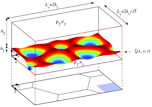
Figure 1: Above: instantaneous realization of hexagaonal Faraday waves in a domain of size $L_{x}\times L_{y}\times(h_{1}+h_{2})$. The density and viscosity are $\rho_{2}$, $\nu_{2}$ above the free surface at $z=\zeta(x,y,t)$; below, they are $\rho_{1}$ and $\nu_{1}$. The displacement amplitude of $\zeta$ is comparable to $h_{1}$; at its lowest points, $\zeta$ almost touches the lower boundary. Below: projection of the horizontal doubly periodic rectangular domain of dimensions $L_{x}\times L_{y}=2\lambda_{c}/\sqrt{3}\times 2\lambda_{c}$ shows that it is compatible with a hexagonal lattice. The minima of $\zeta$ (above) are located at the vertices and centers of the hexagons (below). The right corner represents a portion of the rectangular computational grid; the actual grid is twice as fine in each direction.

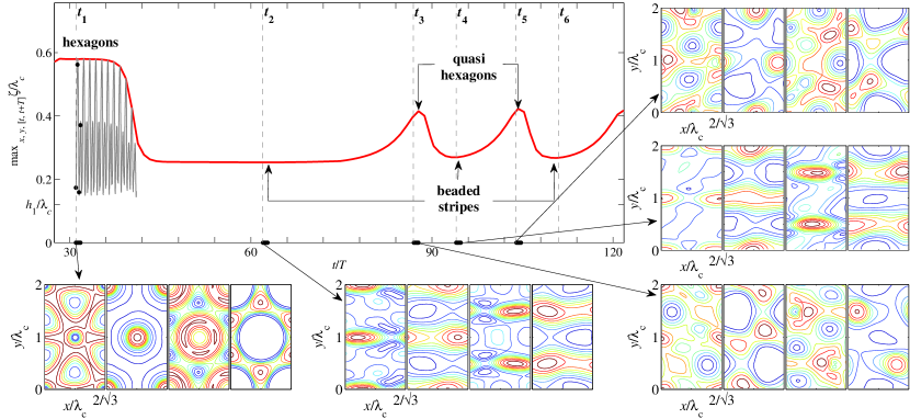
Figure 2: Maximum interface heights $\max_{x,y}\zeta(x,y,t)$ (rapidly oscillating curve) and $\max_{x,y,[t,t+T]}\zeta(x,y,t)$ (smooth envelope). Surrounding visualizations show instantaneous contour plots of $\zeta(x,y,t)$ at times indicated by black dots on rapidly oscillating curve and along abscissa. Red/blue colors regions of maximum/minimum interface height. The color map of each contour plot is scaled independently of the others. Over the large white areas, the interface is very close to the bottom and almost flat. Visualizations shown at $t_{i}+jT/4$ for $j=0,1,2,3$ (i.e. over one subharmonic period) for hexagons at $t_{1}$, symmetric and nonsymmetric beaded stripes at $t_{2}$ and $t_{4}$ and quasi-hexagons at $t_{3}$ and $t_{5}$.

The first detailed spatio-temporal experimental measurements of the interface height $z=\zeta(x,y,t)$ were undertaken by Kityk et al. (2005); *KEMW2009. Their optical technique required the two fluid layers to have the same refractive index, which led them to use fluids of similar viscosities and densities: $\rho_{1}=1346\nobreak\mbox{$\;$kg\,m${}^{-3}$}$, $\nu_{1}=5.35\times 10^{-6}\nobreak\mbox{$\;$m${}^{2}$\,s${}^{-1}$}$, $\rho_{2}=949\nobreak\mbox{$\;$kg\,m${}^{-3}$}$, $\nu_{2}=2.11\times 10^{-5}\nobreak\mbox{$\;$m${}^{2}$\,s${}^{-1}$}$ and surface tension $\sigma=35\nobreak\mbox{$\;$mN\,m${}^{-1}$}$. These parameters, especially the density ratio $\rho_{2}/\rho_{1}=0.7$, differ markedly from most studies of Faraday waves, which use air above either water or silicone oil and so have $\rho_{2}/\rho_{1}\approx 0.001$. At rest, the heavy and light fluids occupy heights of $h_{1}=1.6\nobreak\mbox{$\;$mm}$ and $h_{2}=8.4\nobreak\mbox{$\;$mm}$, respectively. The imposed vibration has frequency $f=12\nobreak\mbox{$\;$Hz}$ and the Faraday instability leads to subharmonic standing waves, so that $\zeta(x,y,t)$ oscillates with period $T=2/f=0.1666\nobreak\mbox{$\;$s}$. Floquet analysis Kumar and Tuckerman (1994) for these parameters yields a critical wavelength of $\lambda_{c}=2\pi/k_{c}=13.2\nobreak\mbox{$\;$mm}$, with which the experiments show close agreement Kityk et al. (2005); *KEMW2009. Thus, another atypical feature of this parameter regime is that $h_{1}\ll\lambda_{c}$; see Fig. 1. Floquet analysis also yields a critical acceleration of $a_{c}=25.8\nobreak\mbox{$\;$m\,s${}^{-2}$}=2.63\>g$. Our simulations are carried out at $a=38.0\nobreak\mbox{$\;$m\,s${}^{-2}$}=3.875\>g=1.473\;a_{c}$, for which hexagons were observed experimentally Kityk et al. (2005); *KEMW2009.

We summarize our formulation and the numerical methods used to compute the fluid motion; see Périnet et al. (2009) for a more detailed description. Our computations use a single-fluid model, representing the velocity $\mathbf{u}$ and pressure $p$ over the whole domain on a staggered MAC mesh Harlow and Welch (1965) which is fixed and uniform. The viscosity and density are variable, taking the values $\nu_{1}$, $\rho_{1}$ for the denser lower fluid, $\nu_{2}$, $\rho_{2}$ for the lighter upper fluid and varying over a few gridpoints at the interface. The moving interface, defined by $z=\zeta(x,y,t)$, is computed by a front-tracking Tryggvason et al. (2001)/immersed-boundary Peskin (1977) method on a semi-Lagrangian triangular mesh which is fixed in the horizontal $x$ and $y$ directions and moves along the vertical direction $z$. The interface is advected and the density and viscosity fields updated. The capillary force is computed locally on the Lagrangian mesh and included in the Navier-Stokes equations, which are solved by a projection method. The computations are carried out in the oscillating reference frame of the container by adding a time-periodic vertical acceleration $a\sin(2\pi f\>t)\mathbf{e}_{z}$ to the equations of motion. No-slip boundary conditions are imposed at the top and bottom boundaries, while periodic boundary conditions are used at the vertical boundaries.

The horizontal dimensions of the domain are chosen to accomodate a hexagonal pattern. We take $L_{x}=2\lambda_{c}/\sqrt{3}$ and $L_{y}=2\lambda_{c}$, as shown in Fig. 1, so that large-scale spatial variations are inaccessible. This domain is also compatible with striped or rectangular patterns, as will be discussed below. The simulations were run with a spatial resolution of $N_{x}\times N_{y}\times N_{z}=58\times 100\times 180$. Each horizontal rectangle is subdivided into 64 triangles to represent the interface. To validate the spatial discretization, we repeated the simulations with a finer resolution of $N_{x}\times N_{y}\times N_{z}=75\times 125\times 225$. Although small quantitative changes were seen, the dynamics remained qualitatively unchanged. The timestep is limited by the advective step, taking values varying between $T/24\,000$ for a hexagonal pattern and $T/4000$ for a beaded striped pattern. This makes the simulation of behavior over many subharmonic periods extremely time-consuming.

Figure 3: Time-filtered spatial Fourier spectra $\zeta_{mn}(t_{i})$: hexagons at $t_{1}$, beaded stripes at $t_{2}$, quasi-hexagons at $t_{3}$ and $t_{5}$, nonsymmetric beaded stripes at $t_{4}$ and $t_{6}$.

Starting from zero velocity and an initial random perturbation of the flat interface, our simulations produced a hexagonal pattern which oscillates subharmonically with the same spatio-temporal spectrum as Kityk et al. (2005); *KEMW2009, as detailed in Périnet et al. (2009). In the experiments, hexagons are transient and difficult to stabilize Wagner , competing with squares and disordered states Kityk et al. (2005); *KEMW2009; Wagner et al. (2000); *WMK2003. In our simulations, after about 10 subharmonic periods, we observed a drastic departure from hexagonal symmetry. Figure 2 shows the instantaneous maximum height $\max_{x,y}\zeta(x,y,t)$ and its envelope $\max_{x,y,[t,t+T]}\zeta(x,y,t)$. Surrounding the time-evolution plot are contours of the interface height at representative times over one subharmonic cycle.

At times $t_{1}+jT/4$, the patterns are hexagonal. Each is invariant under rotations by $\pi/3$ and under reflection, for example about $y=n\lambda_{c}$; these operations generate their isotropy subgroup (group of symmetries), which is isomorphic to $D_{6}$. We call the patterns at $t_{2}+jT/4$ beaded stripes. They satisfy the two symmetry relations:

$$\zeta(x,n\lambda_{c}-y)=\zeta(x,y)=\zeta(m\lambda_{c}/\sqrt{3}+\tilde{x}_{0}-x,y+n\lambda_{c})$$ (1)

where $\tilde{x}_{0}\approx\lambda_{c}/(2\sqrt{3})$ is a spatial phase. The second equality in (1) is variously called shift-and-reflect or glide-reflection symmetry. These invariances describe the crystallographic group called pmg or p2mg Wagner et al. (2000); *WMK2003; wal , which is isomorphic to $Z_{2}\times Z_{2}$. At later times, the patterns have no exact symmetries. Nevertheless, the patterns at times $t_{3}+T/4$ and $t_{5}+3T/4$ contain large flat cells surrounded by six small peaks like those at $t_{1}+3T/4$, which lead us to call them quasi-hexagons. Quasi-hexagons at $t_{3}$ and $t_{5}$ appear in two distinct forms, which are related by the spatio-temporal symmetry

$$\zeta(m\lambda_{c}/\sqrt{3}+x_{0}-x,y+y_{0},t_{3}+T/2)=\zeta(x,y,t_{5})$$ (2)

with phases $x_{0}\approx 0.7\lambda_{c}/\sqrt{3}$ and $y_{0}\approx\lambda_{c}/2$. The patterns at $t_{4}$ and $t_{6}$ resemble those at $t_{2}$ but do not satisfy (1); we call these nonsymmetric beaded stripes. These are also related by the spatio-temporal symmetry (2).

a)

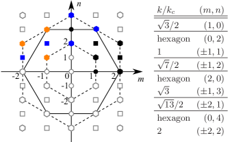
c)

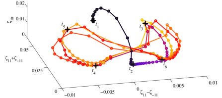
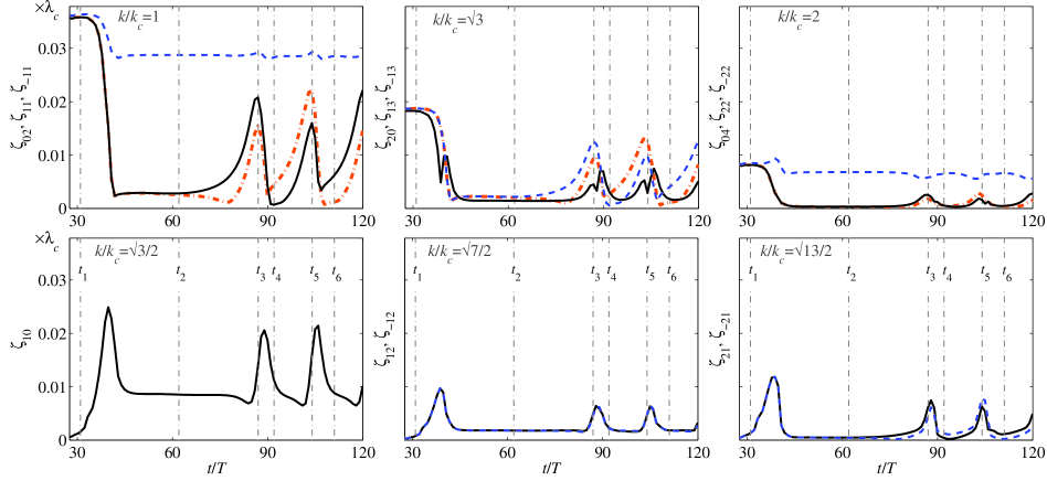
Figure 4: a) Spatial Fourier grid of the domain. Hexagonal symbols: sets of six $\mathbf{k}_{mn}$ which share the same length $k$. This portion of the grid contains three hexagons, with $k/k_{c}=1$, $\sqrt{3}$ and $2$. The hexagonal modes are located at the vertices (and not the sides) of the large hexagons indicated by solid and dashed lines. Square symbols: sets of four $\mathbf{k}_{mn}$ which share the same $k$. Circles: other modes. Colors differentiate between $\mathbf{k}_{mn}$ and its images under rotations of $l\pi/3$ for hexagonal modes or under reflections across the $n$ axis for the others. b) Temporal evolution of $\zeta_{mn}(t)$, grouped by length $k$. The color code is that used in the spatial Fourier grid. Dashed blue curves: hexagonal modes $(0,2)$, $(1,3)$, $(0,4)$ and non-hexagonal modes $(-1,2)$, $(-2,1)$. Solid black curves: hexagonal modes $(1,1)$, $(2,0)$, $(2,2)$ and non-hexagonal modes $(1,0)$, $(1,2)$, $(2,1)$. Dash-dotted orange curves: hexagonal modes $(-1,1)$, $(-1,3)$, $(-2,2)$. c) 3D phase portrait of temporal evolution of modes for an extended simulation. Points are equally spaced in time; their color evolves in time from dark to light. Times $t_{1}\ldots t_{6}$ marked by crosses and by vertical lines in b).

To quantify the behavior in Fig. 2, we have studied the spatial Fourier spectrum. The rectangular box of Fig. 1 constrains the wavevectors to lie on the grid $\mathbf{k}_{mn}\equiv\left(\sqrt{3}m\mathbf{e}_{x}+n\mathbf{e}_{y}\right)k_{c}/2$, $m,n\in\mathbb{Z}$, as shown in Fig. 3 and 4a. We define the time-filtered spatial Fourier transform:

$$\frac{\zeta(\mathbf{x},t)}{\lambda_{c}}=\sum_{m,n}e^{i\mathbf{k}_{mn}\cdot\mathbf{x}}\hat{\zeta}_{mn}(t)\;,\qquad\zeta_{mn}(t)\equiv\max_{[t,t+T]}|\hat{\zeta}_{mn}(t)|$$

In Fig. 3, we plot $\zeta_{mn}(t_{i})$ for $t_{1}\ldots t_{6}$. For the hexagonal pattern at time $t_{1}$ the modes with non-negligeable amplitude are those belonging to hexagons, primarily $(m,n)=(\pm 1,\pm 1)$ and $(0,\pm 2)$, with $k/k_{c}=1$, but also $(\pm 2,0)$ and $(\pm 1,\pm 3)$, with $k/k_{c}=\sqrt{3}$, and $(0,\pm 4)$ and $(\pm 2,\pm 2)$, with $k/k_{c}=2$. The spectrum at $t_{2}$ is dominated by modes $(0,\pm 2)$ and $(\pm 1,0)$, which combine to form the beaded striped patterns – with one bead over $L_{x}$ and two stripes over $L_{y}$ – seen in Fig. 2 at $t_{2}$. The spectra at $t_{3}$ and $t_{5}$ combine wavenumbers seen at $t_{1}$ and $t_{2}$, while those at $t_{4}$ and $t_{6}$ are asymmetric versions of that at $t_{2}$. The spatio-temporal symmetry (2) is manifested by $\zeta_{-m,n}(t_{3,4})=\zeta_{mn}(t_{5,6})$.

Figure 4b shows the time evolution of $\zeta_{mn}(t)$ for the dominant wavevectors, grouping those with the same $k$ value into a single graph. Because $\zeta_{m,-n}=\zeta_{-m,n}$ (resulting from the reality condition $\hat{\zeta}_{m,-n}=\hat{\zeta}^{\ast}_{-m,n}$), we plot only positive $n$. We first describe the evolution of the four most dominant modes in the leftmost column. During the hexagonal phase at $t_{1}$, the only modes with non-negligeable amplitude are those belonging to hexagons. At $t/T\approx 40$, these drop abruptly, with the exception of $\zeta_{02}$. This is accompanied by a burst in amplitude of some of the non-hexagonal modes, notably $\zeta_{10}$, followed by its saturation. Shortly after $t_{2}$, $\zeta_{1,1}$ begins to rise, followed by $\zeta_{-1,1}$; eventually $\zeta_{10}$ rises as well; we conjecture that its growth is fueled by mode interactions arising from $\mathbf{k}_{11}+\mathbf{k}_{-1,-1}+\mathbf{k}_{1,0}=\mathbf{k}_{10}$. By $t_{3}$, these have attained values which approach $\zeta_{02}$, leading to the quasi-hexagonal patterns at $t_{3}$. Mode amplitudes $\zeta_{\pm 1,1}$ then fall quickly, followed by $\zeta_{1,0}$, leading again to a short-lived beaded striped pattern at time $t_{4}$. The cycle then repeats, but this time $\zeta_{-1,1}$ rises before $\zeta_{1,1}$ and attains a higher peak at time $t_{5}$, leading to the difference between the quasi-hexagonal patterns at $t_{5}$ and $t_{3}$. The next cycle shows $\zeta_{11}$ leading again at $t_{6}$. Most of the higher $k$ modes behave like their lower $k$ analogs.

Figure 4c shows a phase portrait, projecting the dynamics onto coordinates, $\zeta_{11}+\zeta_{-1,1}$, $\zeta_{11}-\zeta_{-1,1}$ and $\zeta_{10}$ to represent the dynamics. Here, the simulation has been extended and shows several additional repetitions. The concentration of points indicate that the hexagonal pattern at time $t_{1}$ and the beaded striped pattern at $t_{2}$ are saddles. Afterwards, the trajectory consists of two crossed loops connecting $t_{3}$, $t_{4}$, $t_{5}$ and $t_{6}$. Several dynamical-systems scenarios lead to limit cycles which visit symmetrically related sets, e.g. Hopf bifurcations Clune and Knobloch (1994) or heteroclinic cycles Buono et al. (2000). Since the saddles at $t_{1}$ and $t_{2}$ are not part of the periodic cycle, nor its center, our planned investigation of its origin will be challenging.

A complete analysis of the general bifurcation problem on a hexagonal lattice Buzano and Golubitsky (1983); Golubitsky et al. (1984) shows that the patterns at onset are hexagons and stripes. This analysis of steady states on a hexagonal grid does not apply directly to our study of subharmonic standing waves on the rectangular lattice of Fig. 1. At the other extreme, in large-domain experiments, hexagonal patterns are often observed to undergo other spatio-temporal dynamics, such as competition with squares Kityk et al. (2005); *KEMW2009; Wagner et al. (2000); *WMK2003; Abou et al. (2000), which are inaccessible to current mathematical analysis and to our simulation.

We have observed complex long-time temporal behavior in a fully resolved three-dimensional simulation of Faraday waves in the minimal domain which can accomodate a hexagonal pattern. Although this scenario may prove to be replaced by other dynamics in large domains, we believe that it is of interest in its own right and that it may well be applicable to other pattern-forming systems.

We thank P.-L. Buono and M. Golubitsky for sharing their knowledge of symmetry and C. Wagner for in-depth remarks on experiments. N.P. was partly supported by the Natural Sciences and Engineering Research Council of Canada.

References

- Faraday (1831) M. Faraday, Phil. Trans. R. Soc. Lond. 121, 299 (1831).
- Christiansen et al. (1992) B. Christiansen, P. Alstrøm, and M. T. Levinsen, Phys. Rev. Lett. 68, 2157 (1992).
- Edwards and Fauve (1993) W. S. Edwards and S. Fauve, Phys. Rev. E 47, R788 (1993).
- Kudrolli et al. (1998) A. Kudrolli, B. Pier, and J. P. Gollub, Physica D 123, 99 (1998).
- Rucklidge et al. (2012) A. M. Rucklidge, M. Silber, and A. C. Skeldon, Phys. Rev. Lett. 108, 074504 (2012).
- Périnet et al. (2009) N. Périnet, D. Juric, and L. S. Tuckerman, J. Fluid Mech. 635, 1 (2009).
- Kityk et al. (2005) A. V. Kityk, J. Embs, V. V. Mekhonoshin, and C. Wagner, Phys. Rev. E 72, 036209 (2005).
- Kityk et al. (2009) A. V. Kityk, J. Embs, V. V. Mekhonoshin, and C. Wagner, Phys. Rev. E 79, 029902(E) (2009).
- Kumar and Tuckerman (1994) K. Kumar and L. S. Tuckerman, J. Fluid Mech. 279, 49 (1994).
- Harlow and Welch (1965) F. H. Harlow and J. E. Welch, Phys. Fluids 8, 2182 (1965).
- Tryggvason et al. (2001) G. Tryggvason, B. Bunner, A. Esmaeeli, D. Juric, N. Al-Rawahi, W. Tauber, J. Han, and Y.-J. Jan, J. Comput. Phys. 169, 708 (2001).
- Peskin (1977) C. S. Peskin, J. Comput. Phys. 25, 220 (1977).
- (13) C. Wagner, private communication.
- Wagner et al. (2000) C. Wagner, H. W. Müller, and K. Knorr, Phys. Rev. E 62, R33 (2000).
- Wagner et al. (2003) C. Wagner, H. W. Müller, and K. Knorr, Phys. Rev. E 68, 066204 (2003).
- (16) http://en.wikipedia.org/wiki/Wallpaper_group.
- Clune and Knobloch (1994) T. Clune and E. Knobloch, Physica D 74, 151 (1994).
- Buono et al. (2000) P.-L. Buono, M. Golubitsky, and A. Palacios, Physica D 143, 74 (2000).
- Buzano and Golubitsky (1983) E. Buzano and M. Golubitsky, Phil. Trans. R. Soc. A 308, 617 (1983).
- Golubitsky et al. (1984) M. Golubitsky, J. Swift, and E. Knobloch, Physica D 10, 249 (1984).
- Abou et al. (2000) B. Abou, J.-E. Wesfreid, and S. Roux, J. Fluid Mech. 416, 217 (2000).