The Coronal Abundance Anomalies of M Dwarfs

Abstract

We analyze Chandra X-ray spectra of the M0 V+M0 V binary GJ 338. As quantified by X-ray surface flux, these are the most inactive M dwarfs ever observed with X-ray grating spectroscopy. We focus on measuring coronal abundances, in particular searching for evidence of abundance anomalies related to First Ionization Potential (FIP). In the solar corona and wind, low FIP elements are overabundant, which is the so-called “FIP effect.” For other stars, particularly very active ones, an “inverse FIP effect” is often observed, with low FIP elements being underabundant. For both members of the GJ 338 binary, we find evidence for a modest inverse FIP effect, consistent with expectations from a previously reported correlation between spectral type and FIP bias. This amounts to strong evidence that all M dwarfs should exhibit the inverse FIP effect phenomenon, not just the active ones. We take the first step towards modeling the inverse FIP phenomenon in M dwarfs, building on past work that has demonstrated that MHD waves coursing through coronal loops can lead to a ponderomotive force that fractionates elements in a manner consistent with the FIP effect. We demonstrate that in certain circumstances this model can also lead to an inverse FIP effect, pointing the way to more detailed modeling of M dwarf coronal abundances in the future.

1 INTRODUCTION

The solar corona and solar wind exhibit a curious abundance pattern in which the abundance of an element relative to its abundance in the photosphere is dependent on its first ionization potential (FIP). Elements with low FIP (Fe, Mg, Si, etc.) are found to have coronal abundances that are enhanced relative to elements with high FIP (C, N, O, Ne, etc.), by about a factor of four on average (von Steiger et al., 1995; Feldman & Laming, 2000). This abundance anomaly has been called the “FIP effect,” which at least on the Sun is known to be due to enhancement of low-FIP elements relative to photospheric abundances, as opposed to depletion of high-FIP elements. This phenomenon has been the subject of many theoretical studies. Some of these attribute it to the effects of Alfvén waves passing through the solar atmosphere, which may also be involved in coronal heating (Laming, 2004, 2009, 2012). In addition to its presence on the Sun, evidence for a FIP effect has also been found for some stars of low to moderate activity (Laming et al., 1996; Drake et al., 1997; Laming & Drake, 1999). However, on very active stars the FIP effect tends to be either absent, or sometimes an inverse FIP effect is observed, where low-FIP elements have coronal abundances that are depleted relative to the high-FIP elements (Audard et al., 2001, 2003; Brinkman et al., 2001; Güdel et al., 2001; Huenemoerder et al., 2001, 2003; Sanz-Forcada et al., 2003, 2009; Ball et al., 2005). So far this behavior is not captured in any theoretical model. However, the generalization of the Laming (2009, 2012) models to include other MHD wave modes is expected to yield an inverse FIP effect in the appropriate conditions, within the same framework as that for the FIP effect.

The impression these results provide is of coronal abundances being primarily dependent on stellar activity, with FIP effect changing to inverse FIP as activity increases. However, if only main sequence stars are considered, and if extremely active stars with X-ray luminosities of $\log{L_{X}}>29$ (in ergs s^-1) are excluded, then all activity dependence disappears, and one instead sees a strong dependence on spectral type (Wood & Linsky, 2010, hereafter WL10). In this correlation, early G stars all have a solar-like FIP effect, which decreases towards late G and early K stars, reaching no FIP effect at all at a spectral type of K5 V. Later than K5 V, inverse FIP effects are observed, with the magnitude of the effect increasing with spectral type. We will refer to this as the “FIP-Bias/Spectral-Type” (FBST) relation. This suggests that for the vast majority of cool stars in the Galaxy, coronal abundances are determined entirely by spectral type, and not stellar age or activity. This illustrates the problems inherent in the dominance of very active stars in the archives of X-ray spectra. The stars that are brightest and most easily observed by X-ray observatories are not necessarily representative of the Galactic stellar population as a whole, and therefore may provide a misleading picture of the nature of X-ray emitting stellar coronae.

The FBST relation of WL10 has an important implication for M dwarfs. It implies that all M dwarf coronae should possess an inverse FIP effect. Relatively inactive stars (with $\log{L_{X}}<29$) that follow the FBST relation should have it, and if there is an activity dependence of FIP bias for the most active M dwarfs, experience suggests that this would only act to increase the inverse FIP effect even further.

One problem with verifying this prediction for M dwarfs is that only relatively active M dwarfs can be observed. This is a problem to some degree for all stars, of course, but the problem is magnified for M dwarfs because of their small size. Consider Proxima Centauri (M5.5 Ve), which is by any measure the most inactive M dwarf previously observed spectroscopically in X-rays. With an X-ray luminosity of $\log L_{X}=27.22$ (Schmitt & Liefke, 2004) it is only by virtue of its incomparable close proximity ($d=1.3$ pc) that it can be observed spectroscopically at all. However, although Proxima Cen seems quite inactive as quantified by $L_{X}$, this is not the case if one quantifies activity by surface X-ray flux, $F_{X}$. With a radius of only 0.15 R_⊙ (Ségransan et al., 2003), Proxima Cen’s low X-ray luminosity translates to a relatively high X-ray surface flux of $\log F_{X}=6.08$ (in ergs cm^-2 s^-1). This $F_{X}$ is higher than that of most of the stars that WL10 used to define the FBST correlation, though still lower than all the other M dwarfs. Proxima Cen is the most inactive M dwarf known to possess an inverse FIP effect, but its relatively high $F_{X}$ value leaves open the possibility that at sufficiently low $F_{X}$, the inverse FIP effects of the M dwarfs will drift towards a more solar-like FIP effect.

Our primary goal in this paper is to analyze new Chandra spectra of the GJ 338 binary (M0 V+M0 V), consisting of two M dwarfs with $F_{X}$ much lower than Proxima Cen. We aim to determine whether the GJ 338 coronae possess the expected inverse FIP effect. If it does, this would further demonstrate that the inverse FIP phenomenon is not solely or even primarily an effect of high activity. It would also provide crucial support for the universality of the FBST relation for inactive and modestly active main sequence stars, and provide evidence that all M dwarf coronae exhibit the inverse FIP effect.

2 X-RAY IMAGING OF THE GJ 338 SYSTEM

Our target, GJ 338, was chosen for its close proximity ($d=5.81$ pc) and modest activity level, with an X-ray flux just high enough to be observable spectroscopically. The binarity of the target also makes it attractive, as it allows two relevant stellar spectra to be taken in a single exposure. The only previous X-ray observation to resolve the binary was by the ROSAT HRI imager, which found X-ray luminosities for GJ 338A and GJ 338B of $\log L_{X}=28.16$ and $\log L_{X}=28.21$, respectively. However, weaker X-ray emission was observed during the ROSAT All-Sky Survey (RASS), which found the binary to have a combined $\log L_{X}=27.85$ (Schmitt & Liefke, 2004).

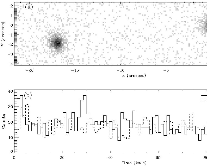
Figure 1: (a) The zeroth-order image of the GJ 338 binary from the Chandra LETGS observation, with GJ 338A being the source on the right. North is up in the figure. An excess of emission seen northwest of GJ 338A is due to an instrumental artifact. (b) X-ray light curves measured for GJ 338A and GJ 338B from the zeroth-order image, using 20 minute time bins.

Chandra observed GJ 338 on 2010 December 29 for 96.5 ksec, using the LETGS setup (LETG grating plus HRC-S detector). An LETGS observation consists of a zeroth-order image plus two identical spectra of the target stretched out to either side of the image along the dispersion direction. The zeroth-order image is shown in Figure 1a, showing the two members of the binary with roughly equal brightness. The measured position angle and stellar separation for the binary is $\theta=96.41^{\circ}$ and $\rho=17.13^{\prime\prime}$, respectively. X-ray luminosities can be estimated directly from the image, which implies that both stars are much fainter than expected from the ROSAT/HRI luminosities quoted above. From the spectra discussed below we measure X-ray luminosities within $5-120$ Å ($0.1-2.4$ keV) of $\log L_{X}=27.64$ and $\log L_{X}=27.60$ for GJ 338A and GJ 338B, respectively, values lower than expected from the HRI observation, but consistent with the RASS luminosity quoted above. In order to quantify $F_{X}$ for these stars, we use Grossman et al. (1974) to estimate radii of 0.59 R_⊙ and 0.58 R_⊙ for GJ 338A and GJ 338B, respectively, leading to surface fluxes of $\log F_{X}=5.31$ and $\log F_{X}=5.29$, values about a factor of 6 lower than $F_{X}$ for Proxima Cen.

The zeroth-order images are also useful for quantifying source variability, and Figure 1b shows light curves for the two stars. The secondary shows no significant X-ray variability, but a couple short flares are apparent on the primary. Such X-ray flaring is quite common for M dwarfs (e.g., Osten et al., 2005; Kowalski et al., 2009).

The GJ 338A image in Figure 1a appears to be asymmetric, especially compared with that of GJ 338B. In particular, there is excess emission NNW of GJ 338A. However, we have determined this to be caused by a recently identified instrumental artifact of the HRC-S detector, which is worth bringing to the attention of other HRC-S users. In short, the region of the HRC-S detector on which GJ 338A ended up located has been found to have unique problems with event positions, confirmed by HRC-S observations of the Chandra calibration target HZ 43 (B. Wargelin, private communication). As part of its system of identifying the centroids of charge clouds induced by X-ray photons, the HRC-S detector uses charge amplifiers called “taps” (Chappell & Murray, 1989; Juda et al., 2000). The dithering pattern used during the course of our LETGS observation carried GJ 338B across taps numbered 98 and 99, while GJ 338A was covered by taps 98–100. It is tap number 100 that is the problem, which therefore affected GJ 338A without affecting GJ 338B. The aimpoint for HRC-S has drifted with time, so it is only recently that this problematic region of the detector has moved to such a disadvantageous location. Note that the spectra themselves do not fall on this part of the detector, so they are unaffected.

3 X-RAY SPECTROSCOPY OF THE GJ 338 SYSTEM

For GJ 338, obtaining spectra from the LETGS data requires a certain amount of specialized data processing, in order to extract separate spectra for each member of the binary. We follow procedures similar to ones used in past analyses of binary stars observed by LETGS (Wood & Linsky, 2006), and we refer the reader to those analyses for details about this data processing. The spectra are processed using version 4.3 of the CIAO software. Although LETGS provides very broad spectral coverage from $5-175$ Å, we find that we are only able to detect the strongest emission lines from these stars, which are below 35 Å. Thus, the decreasing spatial resolution with wavelength exhibited by LETGS spectra is not a concern, so to maximize signal-to-noise for the detected lines we use a relatively narrow extraction window of 16 pixels in the cross-dispersion direction.

Figure 2 shows the resulting spectra, which have been rebinned by a factor of 5 and smoothed slightly to better reveal the emission lines in the noisy data. There are only eight emission features that can be discerned. Table 1 lists counts and line fluxes measured for these lines, some of which are actually blends of multiple lines.

Our principle aim here is to measure the FIP bias present in the coronae of the two GJ 338 stars. Ideally, this requires a full emission measure analysis of line fluxes, as described by WL10. However, with only a limited number of lines to work with, such an analysis is clearly impossible here. We instead estimate a FIP bias from only the strongest lines in the spectrum, those of Fe XVII and O VIII. Since Fe is a low-FIP element while O is a high-FIP element, the Fe XVII/O VIII flux ratio provides a reasonable estimate of FIP bias, particularly since both Fe XVII and O VIII are formed at about the same temperature of $\log T=6.6$.

Between $15-17$ Å, coronal spectra are typically dominated by five lines of Fe XVII, at rest wavelengths of 15.015 Å, 15.262 Å, 16.778 Å, 17.053 Å, and 17.098 Å (Telleschi et al., 2005; Wood & Linsky, 2006, 2010). In the smoothed spectra in Figure 2, these lines coalesce into two blended Fe XVII features. In order to explore how Fe XVII/O VIII varies with FIP bias, we use the sample of stars studied by WL10. A list of these stars is provided in Table 2, with the addition of a few extra ones (particularly $\alpha$ Cen AB), as described below. For the WL10 stars, we sum the fluxes of the Fe XVII lines and divide the sum by the line flux observed for the H-like O VIII Lyman-$\alpha$ line at 18.97 Å, yielding a final Fe XVII/O VIII ratio. These ratios incorporate spectral measurements and analyses by Ness et al. (2003), Telleschi et al. (2005), and Liefke et al. (2008).

The FIP biases defined by WL10 ($F_{bias}$) are listed in Table 2 and plotted versus the Fe XVII/O VIII ratios in Figure 3. As described in detail by WL10, the $F_{bias}$ number represents an attempt to quantify the FIP bias in a stellar corona in a single number that considers abundance measurements of four high-FIP elements (C, N, O, and Ne) and the best reference low-FIP element, Fe. For each of the four high-FIP elements we take the logarithmic abundance ratio with Fe, minus the assumed photospheric ratio, i.e., $\log{\rm[X/Fe]}-\log{\rm[X/Fe]}_{*}$. The average of these four quantities is $F_{bias}$. No photospheric abundance measurements are available for the M dwarfs in the sample, including GJ 338, so we simply have to assume solar photospheric abundances apply. Asplund et al. (2009) is used as the source of solar abundances, but for reasons described in detail in WL10, we replace the Ne abundance with the one suggested by the average coronal Ne/O ratio measured by Drake & Testa (2005). For the GK dwarfs, stellar photospheric abundances from Allende Prieto et al. (2004) are used, but these abundances are measured relative to solar ones, so even for these stars the assumed reference solar abundances must be used to compute $\log{\rm[X/Fe]}_{*}$.

As quantified this way, $F_{bias}=0$ corresponds to coronal abundance ratios being identical (on average) to photospheric ratios, $F_{bias}<0$ corresponds to a solar-like FIP effect, and $F_{bias}>0$ corresponds to an inverse FIP effect. It is important to realize that the coronal abundances quantified by $F_{bias}$ are relative abundances, not absolute ones. Computing absolute abundances, i.e., relative to H, requires an additional analysis of line-to-continuum ratio, which represents a substantial source of systematic error. Sticking with relative abundances allows us to avoid inserting this uncertainty into the $F_{bias}$ quantity, but it does mean that, for example, $F_{bias}<0$ does not tell you whether the low-FIP elements are being enhanced in the corona (as in the case of the Sun) or if the high-FIP elements are being depleted.

Figure 3 shows that for the WL10 sample of stars there is a strong correlation between $F_{bias}$ and Fe XVII/O VIII. This is quantified by a second order polynomial fit, where if $x\equiv\log{({\mbox{\rm Fe~{}XVII/O~{}VIII}})}$, $F_{bias}=0.344-1.926x+0.994x^{2}$. Thus, for GJ 338A and GJ 338B, we can measure Fe XVII/O VIII ratios from Table 1 and then infer $F_{bias}$ from the polynomial fit in Figure 3. Error boxes in Figure 3 show the results independently for GJ 338A and GJ 338B. However, given that Fe XVII/O VIII is so similar for the two stars, and given that they have the same spectral type, we deem it worthwhile to simply sum the line fluxes of the two stars and compute a single Fe XVII/O VIII ratio and $F_{bias}$ value for GJ 338AB. The result, $x=0.020\pm 0.130$ and $F_{bias}=0.31^{+0.26}_{-0.23}$, is shown in the figure as well. For GJ 338AB we find that $F_{bias}>0$, indicating an inverse FIP effect. If stellar activity is quantified by $F_{X}$, the GJ 338 stars are now easily the least active stars known to have an inverse FIP effect present in their coronae.

There is an important caveat about the correlation between $F_{bias}$ and Fe XVII/O VIII in Figure 3: the relation is inferred from a particular sample of moderately active stars with similar emission measure distributions. Stars with coronal temperatures much different than these may not be consistent with this relation. In order for this relation to be applicable to GJ 338AB, we need to have reason to believe that GJ 338AB’s coronal temperatures are comparable to those of the WL10 sample of stars. The best diagnostic of coronal temperature available to us for GJ 338AB is the flux ratio of the O VIII and O VII lines in Table 1. Uncertainties in the individual line measurements are very high, but if the O VIII line fluxes for both stars are summed, and then divided by the sum of all O VII lines from both stars, the result is a flux ratio of O VIII/O VII=0.8. These ratios are near the lower bound observed within the WL10 sample. They are still comparable, though, being particularly close to the ratio seen for 36 Oph B, for example (see Wood & Linsky, 2006), suggesting similar coronal temperatures. Thus, we think the $F_{bias}$ measurement for GJ 338AB provided by Figure 3 should be good to within the broad error bars. In contrast, we note in passing that line measurements from LETGS spectra of $\alpha$ Cen A and B (G2 V+K1 V) by Raassen et al. (2003) imply that these inactive stars have much lower O VIII/O VII ratios, indicative of much cooler coronae, and as a consequence their $F_{bias}$ values are not consistent with the relation in Figure 3 (see Table 2 and discussion below), demonstrating that not all stars will follow this relation.

In order to put the new measurement into context, we have in Table 2 compiled a list of $F_{bias}$ quantities that can be computed from past coronal abundance analyses of X-ray spectra, keeping in mind that we are interested in main sequence stars with $\log L_{X}<29$. This mostly consists of the WL10 sample of stars, but as that paper did not provide a tabulated list of stars and $F_{bias}$ numbers, we take the opportunity to do so here. To the WL10 sample, we add $\alpha$ Cen AB (G2 V+K1 V) from Raassen et al. (2003), and our new GJ 338AB result. Finally, at the bottom of the table, we list a few representative very active stars with $\log L_{X}>29$, which we will use to illustrate how the coronal abundances of such stars behave differently from the less active main sequence stars.

The fourth column of Table 2 lists radii for our sample of stars. For most of the G and K dwarfs, the radii are computed using the Barnes-Evans relation (Barnes et al., 1978), except for $\alpha$ Cen A and B, for which direct measurements of radii are available (Kervella et al., 2003). With the exception of GJ 338AB and Proxima Cen, whose radii have already been discussed earlier, we use Morin et al. (2008) as the source for the stellar radii of the M dwarfs. The X-ray luminosities in column 5 of Table 2 are for the ROSAT PSPC bandpass of $0.1-2.4$ keV, and most are from ROSAT PSPC measurements made during the ROSAT All-Sky Survey (Schmitt & Liefke, 2004). For the Sun, we assume $\log L_{X}=27.35$, the middle of the range computed by Judge et al. (2003). Ayres (2009) estimate that $\alpha$ Cen A and B have average X-ray fluxes about a factor of two below and above that of the Sun, respectively, so that is what is assumed for $\alpha$ Cen AB in Table 2. The sixth column lists X-ray surface fluxes computed from the X-ray luminosities and stellar radii listed in columns four and five.

The last column of Table 2 lists the references for the coronal abundance analyses for these stars. There are two different quantifications of coronal FIP bias listed in the table. The first is a simple coronal Ne/Fe abundance ratio, with no attempt to normalize this to any assumed photospheric abundances. And finally, of course, the more complex $F_{bias}$ quantity that we have described in detail above. Although we use coronal abundances measured by others, in computing $F_{bias}$ we are careful to apply our own self-consistent assumptions about assumed reference photospheric abundances, as described above. Allende Prieto et al. (2004) is the source for all the photospheric abundances assumed for the G and K stars, except for EK Dra and AB Dor, for which we simply rely on the same photospheric abundances assumed in the original coronal abundance analysis.

Figure 4a reproduces the FBST relation from WL10, but with the addition of extra data points. These include our new GJ 338AB data point, which is nicely consistent with the relation. The addition of $\alpha$ Cen A and B appears to significantly increase the scatter, suggesting that $\alpha$ Cen AB may be somewhat discrepant. It is possible that this is because these stars are significantly less active and have significantly cooler coronae than any of the other stars in the sample, except for the Sun. Finally, the three representative very active stars listed in Table 2 are also plotted in Figure 4a, demonstrating that stars with $\log L_{X}>29$ lie above the FBST relation defined by the less active stars.

Figure 4b is analogous to Figure 4a, but uses the simpler FIP bias indicator, the coronal Ne/Fe ratio. One purpose of this figure is to demonstrate that even with a simpler FIP bias quantifier, with no attempt whatsoever to normalize to photospheric abundances, you can still see the same correlation in Figure 4b as in 4a, demonstrating that the FBST correlation is not a product of assumptions about photospheric abundances. Sanz-Forcada et al. (2009) hypothesized that inverse FIP effects reported in the literature might be an artifact of assuming solar photospheric abundances for these stars, as none of these stars have measured photospheric abundances. However, the consistency the M dwarfs show with the overall spectral type dependence in Figure 4 would argue against this interpretation, as do observations of flares in such stars (e.g., EV Lac; Laming & Hwang, 2009), where composition changes during the event, interpreted as the result of chromospheric evaporation, suggest a photospheric composition similar to that of the Sun. Figure 4b also allows us to compare our main sequence Ne/Fe ratios with those measured for T Tauri stars by Güdel et al. (2007). Güdel et al. (2007) reported a spectral type dependence of coronal abundance for T Tauri stars, which parallels the main sequence FBST relation, basically where the very active main sequence stars lie in the figure.

Figures 4c and 4d demonstrate explicitly that in our sample of stars there is no correlation of $F_{bias}$ with activity at all, regardless of whether $\log L_{X}$ or $\log F_{X}$ is used as the activity quantifier. By itself, Figure 4d might suggest that the least active stars tend to have low $F_{bias}$ values, but this is a selection effect. We would argue on the basis of Figure 4a that the upper left corner of Figure 4d is actually full of inactive M dwarfs that are simply too faint to observe spectroscopically in X-rays. The GJ 338AB observation presented here basically represents an attempt to push farther into this corner of Figure 4d. Replacing $\log F_{X}$ with $\log L_{X}/L_{bol}$, which is another commonly used activity diagnostic, yields results qualitatively similar to Figure 4d, but with the M dwarfs shifted further to the right relative to the other stars.

We have been quoting $\log L_{X}=29$ as the boundary between stars that obey the FBST relation and stars that do not, but intuitively one would think that such a border would be better defined in terms of a normalized activity diagnostic like $\log F_{X}$ or $\log L_{X}/L_{bol}$, considering that the sample of stars contains stars of various sizes. However, in Figure 4d it is not easy to clearly draw a vertical line separating the filled symbols (stars that are consistent with the FBST relation) and the open symbols (stars not consistent with the FBST relation). Note that the situation is even worse if $\log L_{X}/L_{bol}$ is plotted instead of $\log F_{X}$, with the M dwarfs even further to the right relative to the other data points. One could perhaps draw the line at $\log F_{X}=7.0$, which would only place EV Lac on the wrong side of the line. Nevertheless, the $\log L_{X}=29.1$ boundary shown in Figure 4c seems to work better, so we will in the future quote $\log L_{X}=29.1$ as the activity threshold where activity dependence of coronal abundances starts to become apparent. (With several stars in our sample right at $\log L_{X}=29.0$, it seems wise to conservatively move the divider to $\log L_{X}=29.1$.)

4 MODELING THE INVERSE FIP EFFECT

One of the striking features of the FBST relation illustrated in Figure 4 is how the coronal abundance anomaly smoothly changes from solar-like FIP bias at spectral types G to early K, to inverse FIP in M dwarfs. This suggests that a model for solar-like FIP fractionation should, with suitably chosen parameters, be capable of predicting an inverse FIP effect. Laming (2004) reviewed the various solar FIP models available at that time, and argued that only the model based on the ponderomotive force arising from MHD waves could also plausibly explain the inverse FIP effect. Here we elaborate on this suggestion and provide a semi-quantitative illustration of how such a model would work. We defer a fuller exposition, designed to match specific stars, to later papers.

The model described by Laming (2004, 2009) and most recently by Laming (2012) for the FIP effect assumes that Alfvén waves of amplitude approximately 50 km s^-1 are generated in a coronal loop at the resonant frequency, and remain trapped in the loop “resonant cavity”. Upon reflection from chromospheric footpoints, the waves develop a ponderomotive force in the steep density gradients there, and this force, acting on chromospheric ions (but not neutrals), preferentially accelerates these ions up into the corona. Laming (2012) studies the fractionations produced by waves on and off resonance, and Rakowski & Laming (2012) extend this to different loop lengths and magnetic fields, concentrating mainly on the fractionation of He with respect to O. These works only consider coronal Alfvén waves, with chromospheric acoustic waves included in an ad hoc manner. When these upcoming chromospheric acoustic waves are allowed to mode convert, at the layer where sound and Alfvén speeds are equal, to what in the magnetically dominated upper chromospheric become fast mode waves, inverse FIP fractionation can result. This arises because the fast mode waves undergo reflection back downwards as the Alfvén speed increases, giving rise to a downwards directed ponderomotive force than can compete with that due to the coronal Alfvén waves.

We treat the fast mode waves as approximately isotropic in the upward moving hemisphere. Then the fraction reflected at chromospheric height $z$ is

$$f_{R}\left(z\right)\simeq\sqrt{1-{c_{s}^{2}\left(z_{\beta=1}\right)\over V_{A}^{2}\left(z\right)+c_{s}^{2}\left(z\right)}}$$ (1)

where $z_{\beta=1}$ is the chromospheric height where mode conversion occurs. The ponderomotive acceleration due to fast mode waves is then

$$a={c^{2}\over 4}{\partial\over\partial z}\left(\delta E^{2}\over B^{2}\right)={\delta v^{2}\over 2}\left(1-f_{R}\right){1\over\delta v}{\partial\delta v\over\partial z}-{\delta v^{2}\over 4}{\partial f_{R}\over\partial z},$$ (2)

where $\delta v$ is the wave amplitude in km s^-1. The two terms represent an upwards contribution arising as the fast mode waves increase in amplitude as they propagate through lower density plasma, and the downwards contribution arising from fast mode wave reflection. Evaluating

$${\partial f_{R}\over\partial z}={c_{s}^{2}\left(z_{\beta=1}\right)V_{A}\over\left(V_{A}^{2}+c_{s}^{2}\right)^{2}f_{R}}{\partial V_{A}\over\partial z}={c_{s}^{2}\left(z_{\beta=1}\right)V_{A}^{2}\over\left(V_{A}^{2}+c_{s}^{2}\right)^{2}f_{R}}\left({1\over H_{B}}-{1\over 2H_{D}}\right)$$ (3)

and assuming from the WKB approximation

$${1\over\delta v}{\partial\delta v\over\partial z}={-1\over 2H_{B}}-{1\over 4H_{D}},$$ (4)

where $H_{D}$ and $H_{B}$ are the signed density and magnetic field scale heights, we find

$$a={\delta v^{2}\over f_{R}}\left\{\left(f_{R}-1\right)\left(-{1\over 8H_{D}}-{1\over 4H_{B}}\right)+{c_{s}^{2}\left(z_{\beta=1}\right)\over\left(V_{A}^{2}+c_{s}^{2}\right)^{2}}\left(-{c_{s}^{2}\over 8H_{D}}-{c_{s}^{2}\over 4H_{B}}-{V_{A}^{2}\over 2H_{B}}\right)\right\}.$$ (5)

Remembering that both $H_{D}$ and $H_{B}$ are negative, and $f_{R}<1$, the first term in curly brackets is negative, giving rise to an inverse FIP effect, and the second term is positive, giving the more usual FIP effect. In conditions where $V_{A}>>c_{s}$, we expand $f_{R}$ as a Taylor series in the small quantity $c_{s}^{2}/V_{A}^{2}$, and to leading order in this quantity find that an overall downwards pointed ponderomotive acceleration requires $\left|H_{D}\right|<\left|H_{B}\right|/6$ in this simple model.

Additional reflection of fast mode waves from, e.g., density fluctuations (not included in this model) would relax the requirement. So too would fast mode waves spreading out laterally from a horizontally localized source. Even so, equation (5) implies that inverse FIP effect is more likely to be found in stars with minimal magnetic field expansion through the chromosphere, consistent with observations of active M dwarfs. While the magnetic fields measured in such stars are similar to those in the Sun, the filling factor is higher (e.g., Donati & Landstreet, 2009), allowing less volume for expansion with increasing altitude. However, it is less certain whether this argument applies to less active M dwarfs like GJ 338AB.

These fast mode wave are assumed to derive from mode conversion of $p$-modes at this layer. The acoustic waves have an energy transmission coefficient of (Cally & Goossens, 2008)

$$T=\exp\left(-\pi\left|{\bf k}\right|\sec\theta\sin^{2}\theta\over\left[d\left(V_{A}^{2}/c_{s}^{2}\right)/dz\right]_{\beta=1}\right)$$ (6)

in vertical magnetic field, where $\theta$ is the polar angle of the wavevector. Similarly to the Alfvén waves, we model the acoustic wave energy density $U_{ac}$ associated with the fast mode wave energy density $U_{fm}$ by $U_{ac}\left(z\right)=6U_{fm}\left(z_{\beta=1}\right)c_{s}\left(z\right)^{2}/V_{A}\left(z\right)^{2}$. The factor of 6 is chosen to match the acoustic and Alfvén or fast mode amplitudes given in Cranmer et al. (2007) and Khomenko & Cally (2011), and is consistent with equation (6) for $\left|k\right|/\left[d\left(V_{A}^{2}/c_{s}^{2}\right)/dz\right]_{\beta=1}=0.145$ when $\theta=32^{\circ}$. The last factor of $c_{s}\left(z\right)^{2}/V_{A}\left(z\right)^{2}$ approximates the continuing reflection of acoustic waves by the increasing cut off frequency above the mode conversion layer (see, e.g., Barnes & Cally, 2001).

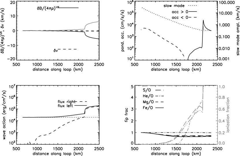
Figure 5: Illustration of a model for the inverse FIP effect, which can be compared with Figure 3 from Laming (2012) illustrating a model for a solar-like FIP effect. The top left panel shows the variables $\delta v$ and $\delta B/\sqrt{4\pi\rho}$ for the coronal Alfvén wave, with black and gray lines corresponding to real and imaginary parts. The bottom left panel shows the upgoing (dashed curve) and downgoing (solid curve) wave energy fluxes. The dotted line shows their difference, and should be horizontal in the absence of wave growth or damping, if energy is conserved. The top right panel shows the ponderomotive acceleration. The positive contribution in the upper chromosphere (solid curve) comes from the coronal Alfvén waves. The negative contribution lower down (dashed curve) comes from the total internal reflection of fast mode waves. The dotted curve gives the amplitude of acoustic waves through the chromosphere. The gray lines in the bottom right panel show ionization fractions for S, He, Mg, and Fe, with the extra triple-dot-dashed line showing O as well. The Mg and Fe ionization fractions are both near 1 throughout the loop. Most importantly, the solid lines show various abundance ratios: He/O remains unchanged, but all others indicate an inverse FIP effect.

Figure 5 illustrates a calculation designed to give an inverse FIP effect. The figure is analogous to Figure 3 of Laming (2012), which illustrates a model of a solar-like FIP effect. A loop of length 100,000 km, with a 100 G magnetic field is considered. The magnetic field is uniform through the chromosphere, and a fast mode wave amplitude of 20 km s^-1 is included at the $\beta=1$ layer, which is allowed to propagate and refract as described above. The model chromosphere derives from the solar model of Avrett & Loeser (2008). Future work should implement a model stellar chromosphere. The top left panel shows the variation of the perturbations $\delta v$ and $\delta B/\sqrt{4\pi\rho}$ associated with the coronal Alfvén wave, and the bottom left panel shows the Alfvén wave energy fluxes, both upward and downwards directed. The dotted line in the bottom right panel shows the difference in wave energy fluxes, and should be horizontal in the absence of wave damping or growth if energy is conserved. The top right panel shows the ponderomotive acceleration. The positive contribution in the upper chromosphere (solid curve) comes from the coronal Alfvén waves. The negative contribution lower down (dashed curve) comes from the total internal reflection of fast mode waves. The dotted curve gives the amplitude of acoustic waves through the chromosphere, modeled as outlined above. The bottom right panel gives the FIP fractionations for the ratios S/O, He/O, Mg/O and Fe/O. The He/O ratio remains unchanged, but all others display an inverse FIP effect.

The transition from FIP effect to inverse FIP effect with increasing fast mode wave amplitude at the $\beta=1$ layer is illustrated in Table 3. In the absence of fast mode waves, a small FIP effect results, with the inverse FIP effect becoming gradually more dominant as amplitude increases.

5 SUMMARY

We have analyzed Chandra observations of the GJ 338AB binary, representing the least active M dwarfs ever observed spectroscopically in X-rays. Our results are summarized as follows:

1. Despite the limited number of lines detected in the spectra, we demonstrate that the coronae of the two GJ 338 stars exhibit an inverse FIP effect, making these the least active stellar coronae known to show this phenomenon.

2. The inverse FIP effect observed for GJ 338AB is consistent with expectations from the FBST relation of WL10, which suggests that all M dwarfs, both active and inactive, should exhibit an inverse FIP effect.

3. A compilation of coronal abundance measurements for main sequence stars (beyond that of WL10) is used to demonstrate that these stars exhibit no significant correlation between coronal abundance and activity, regardless of whether $\log L_{X}$ or $\log F_{X}$ is used as the activity diagnostic.

4. Past work has demonstrated that MHD waves propagating through coronal loops can generate a ponderomotive force capable of fractionating elements in a manner consistent with the solar-like FIP effect (Laming, 2004, 2009, 2012). Building on this theoretical framework, we have shown that such models can also yield an inverse FIP effect in certain circumstances, depending on where MHD waves in the stellar atmosphere are generated, and on where they are transmitted and reflected. In particular, waves propagating upward from the chromosphere and reflecting back down rather than down from the corona and reflecting back up tend to lead to inverse FIP. In the future, we will develop models specifically tailored for M dwarfs such as GJ 338AB, in order to explore in more detail what characteristics of M dwarf atmospheres lead their coronae to have an inverse FIP effect instead of a solar-like FIP effect.

Table 1: Chandra Line Measurements

Ion	$\lambda_{obs}$	Counts		Flux (10-5 ph cm-2 s-1)
	(Å)	GJ 338A	GJ 338B	GJ 338A	GJ 338B
Ne IX	13.6	$75.8\pm 27.1$	$48.8\pm 27.1$	$2.81\pm 1.00$	$1.81\pm 1.00$
Fe XVII	15.1	$34.3\pm 22.9$	$40.2\pm 26.7$	$1.25\pm 0.84$	$1.47\pm 0.98$
Fe XVII	17.0	$58.6\pm 24.1$	$61.6\pm 21.5$	$2.47\pm 1.02$	$2.60\pm 0.91$
O VIII	19.0	$81.3\pm 21.7$	$89.6\pm 20.6$	$3.44\pm 0.92$	$3.77\pm 0.87$
O VII	21.6	$50.4\pm 22.4$	$29.7\pm 21.7$	$3.29\pm 1.46$	$1.92\pm 1.40$
O VII	22.1	$33.1\pm 18.7$	$20.8\pm 18.3$	$2.20\pm 1.24$	$1.38\pm 1.21$
N VII	24.8	$35.2\pm 20.1$	$34.4\pm 21.5$	$2.39\pm 1.36$	$2.33\pm 1.46$
C VI	33.7	$41.8\pm 20.4$	$22.8\pm 14.3$	$3.79\pm 1.85$	$2.06\pm 1.29$

Table 2: List of FIP Bias Assessments for Main Sequence Stars

Star	Alternate	Spectral	Radius	$\log L_{X}$	$\log F_{X}$	Ne/Fe	$F_{bias}$	Ref.
	Name	Type	(R⊙)	(ergs s-1)	(ergs cm-2 s-1)
$\beta$ Com	HD 114710	G0 V	1.08	28.21	5.36	0.73	$-0.668$	1
$\pi^{1}$ UMa	HD 72905	G1 V	0.91	28.97	6.27	1.60	$-0.645$	1
$\chi^{1}$ Ori	HD 39587	G1 V	0.98	28.99	6.22	1.91	$-0.555$	1
Sun	…	G2 V	1.00	27.35	4.57	1.02	$-0.600$	2
$\alpha$ Cen A	HD 128620	G2 V	1.22	27.00	4.04	1.41	$-0.410$	3
$\kappa$ Ceti	HD 20630	G5 V	0.98	28.79	6.02	2.51	$-0.462$	1
$\xi$ Boo A	HD 131156A	G8 V	0.83	28.86	6.24	3.80	$-0.344$	4
70 Oph A	HD 165341A	K0 V	0.85	28.27	5.63	2.40	$-0.403$	5
36 Oph A	HD 155886	K1 V	0.69	28.10	5.64	4.90	$-0.250$	5
36 Oph B	HD 155885	K1 V	0.59	27.96	5.63	3.80	$-0.328$	5
$\alpha$ Cen B	HD 128621	K1 V	0.86	27.60	4.95	1.44	$-0.478$	3
$\epsilon$ Eri	HD 22049	K2 V	0.78	28.32	5.75	4.68	$-0.050$	5
$\xi$ Boo B	HD 131156B	K4 V	0.61	27.97	5.62	7.41	$-0.185$	4
70 Oph B	HD 165341B	K5 V	0.66	28.09	5.67	8.71	$0.138$	5
GJ 338AB	…	M0 V+M0 V	0.59+0.58	27.92	5.30	…	$0.305$	6
EQ Peg A	GJ 896A	M3.5 V	0.35	28.71	6.84	16.12	$0.450$	7
EV Lac	GJ 873	M3.5 V	0.30	28.99	7.25	13.92	$0.474$	7
EQ Peg B	GJ 896B	M4.5 V	0.25	27.89	6.31	14.67	$0.417$	7
AD Leo	GJ 388	M4.5 V	0.38	28.80	6.86	18.25	$0.536$	7
Proxima Cen	GJ 551	M5.5 V	0.15	27.22	6.08	11.98	$0.471$	7
Very Active Star Sample ($\log L_{X}>29$)
EK Dra	HD 129333	G1.5 V	0.89	29.93	7.25	3.71	$-0.277$	1
AB Dor	HD 36705	K0 V	0.79	30.06	7.48	17.11	$0.488$	8
AU Mic	HD 197481	M1 V	0.61	29.62	7.27	24.30	$0.695$	7

References. — (1) Telleschi et al. 2005. (2) Feldman & Laming 2000. (3) Raassen et al. 2003. (4) Wood & Linsky 2010 (WL10). (5) Wood & Linsky 2006. (6) This paper. (7) Liefke et al. 2008. (8) Güdel et al. 2001.

Table 3: Modeled Coronal Abundance Ratios

Ratio	Fast Mode Wave Amplitude
	0 km s-1	5 km s-1	10 km s-1	20 km s-1
He/O	0.98	0.98	0.98	0.98
C/O	1.00	1.00	1.00	1.00
N/O	1.00	1.00	1.00	1.00
Ne/O	1.00	1.00	1.00	1.00
Mg/O	1.04	0.90	0.80	0.70
Si/O	1.04	0.89	0.80	0.71
Ar/O	1.00	1.00	1.00	1.00
Ca/O	1.06	0.89	0.79	0.68
Fe/O	1.07	0.88	0.78	0.67

Figure 2: Chandra LETGS X-ray spectra of GJ 338A and GJ 338B. The wavelength is in Ångstroms.

Figure 3: The coronal FIP bias, $F_{bias}$, is plotted versus the logarithmic flux ratio of Fe XVII 15–17 Å lines to the O VIII 19.0 Å line, for the sample of moderately active main sequence stars studied by WL10. Values of $F_{bias}<0$ correspond to a solar-like FIP effect, while $F_{bias}>0$ corresponds to an inverse FIP effect. A second-order polynomial has been fitted to these data points (dot-dashed line). Combining this relation with the Fe XVII/O VIII ratios measured for GJ 338 yields the displayed error boxes, which are shown for the binary as a whole, and for each member separately.

Figure 4: (a) A plot of $F_{bias}$ versus spectral type for the WL10 sample of main sequence stars with $\log L_{X}<29$ (diamonds), combined with measurements of $\alpha$ Cen A and B (triangles) and our new measurement for GJ 338AB (circle). See Table 2 for a list of the stars. A strong correlation of $F_{bias}$ with spectral type is apparent, i.e., the FBST relation. The open squares are examples of three main sequence stars above the $\log L_{X}=29$ threshold, all of which lie above the FBST relation seen for the less active stars. (b) The coronal Ne/Fe ratio is plotted versus spectral type for both the Table 2 sample of main sequence stars, and for T Tauri stars from Güdel et al. (2007) (asterisks). (c) Plot of $F_{bias}$ versus X-ray luminosity. A vertical line at $\log L_{X}=29.1$ separates the stars that follow the FBST relation in (a) and those that do not. (d) Plot of $F_{bias}$ versus X-ray surface flux.

References

- Allende Prieto et al. (2004) Allende Prieto, C., Barklem, P. S., Lambert, D. L., & Cunha, K. 2004, A&A, 420, 183
- Asplund et al. (2009) Asplund, M., Grevesse, N., Sauval, A. J., & Scott, P. 2009, ARA&A, 47, 481.
- Audard et al. (2001) Audard, M., Behar, E., Güdel, M., Raassen, A. J. J., Porquet, D., Mewe, R., Foley, C. R., & Bromage, G. E. 2001, A&A, 365, L329
- Audard et al. (2003) Audard, M., Güdel, M., Sres, A., Raassen, A. J. J., & Mewe, R. 2003, A&A, 398, 1137
- Avrett & Loeser (2008) Avrett, E., & Loeser, R. 2008, ApJS, 175, 239
- Ayres (2009) Ayres, T. R. 2009, ApJ, 696, 1931
- Ball et al. (2005) Ball, B., Drake, J. J., Lin, L., Kashyap, V., Laming, J. M., & García-Alvarez, D. 2005, ApJ, 634, 1336
- Barnes et al. (1978) Barnes, T. G., Evans, D. S., & Moffett, T. J. 1978, MNRAS, 183, 285
- Barnes & Cally (2001) Barnes, G., & Cally, P. S. 2001, Publ. Astron. Soc. Aust., 18, 243
- Brinkman et al. (2001) Brinkman, A. C., et al. 2001, A&A, 365, L324
- Cally & Goossens (2008) Cally, P. S., & Goossens, M. 2008, Solar Phys., 251, 251
- Chappell & Murray (1989) Chappell, J. H., & Murray, S. S. 1989, Proc. SPIE, 1159, 460
- Cranmer et al. (2007) Cranmer, S. R., van Ballegooijen, A. A., & Edgar, R. J. 2007, ApJS, 171, 520
- Donati & Landstreet (2009) Donati, J.-F., & Landstreet, J. D. 2009, ARAA, 47, 333
- Drake et al. (1997) Drake, J. J., Laming, J. M., & Widing, K. G. 1997, ApJ, 478, 403
- Drake & Testa (2005) Drake, J. J., & Testa, P. 2005, Nature, 436, 525
- Feldman & Laming (2000) Feldman, U., & Laming, J. M. 2000, Phys. Scr., 61, 222
- Goodman (2011) Goodman, M. L. 2011, ApJ, 735, 45
- Grossman et al. (1974) Grossman, A. S., Hays, D., & Graboske, H. C., Jr. 1974, A&A, 30, 95
- Güdel et al. (2001) Güdel, M., et al. 2001, A&A, 365, L336
- Güdel et al. (2007) Güdel, M., Skinner, S. L., Mel’nikov, S. Y., Audard, M., Telleschi, A., & Briggs, K. R. 2007, A&A, 468, 529
- Huenemoerder et al. (2003) Huenemoerder, D. P., Canizares, C. R., Drake, J. J., & Sanz-Forcada, J. 2003, ApJ, 595, 1131
- Huenemoerder et al. (2001) Huenemoerder, D. P., Canizares, C. R., & Schulz, N. S. 2001, ApJ, 559, 1135
- Juda et al. (2000) Juda. M., Austin, G. K., Chappell, J. H., Gomes, J. J., Kenter, A. T., Kraft, R. P., Murray, S. S., & Zombeck, M. V. 2000, Proc. SPIE, 4140, 155
- Judge et al. (2003) Judge, P. G., Solomon, S. C., & Ayres, T. R. 2003, ApJ,
- Kervella et al. (2003) Kervella, P., Thévenin, F., Ségransan, D., Berthomieu, G., Lopez, B., Morel, P., & Provost, J. 2003, A&A, 404, 1087
- Khomenko & Cally (2011) Khomenko, E., & Cally, P. S. 2011, J. Phys.: Conf. Ser., 271, 012042
- Kowalski et al. (2009) Kowalski, A. F., Hawley, S. L., Hilton, E. J., Becker, A. C., West, A. A., Bochanski, J. J., & Sesar, B. 2009, AJ, 138, 633
- Laming (2004) Laming, J. M. 2004, ApJ, 614, 1063
- Laming (2009) Laming, J. M. 2009, ApJ, 695, 954
- Laming (2012) Laming, J. M. 2012, ApJ, 744, 115
- Laming & Drake (1999) Laming, J. M., & Drake, J. J. 1999, ApJ, 516, 324
- Laming et al. (1996) Laming, J. M., Drake, J. J., & Widing, K. G. 1996, ApJ, 462, 948
- Laming & Hwang (2009) Laming, J. M., & Hwang, U. 2009, ApJ, 707, L60
- Liefke et al. (2008) Liefke, C., Ness, J. -U., Schmitt, J. H. M. M., & Maggio, A. 2008, A&A, 491, 859
- Morin et al. (2008) Morin, J., et al. 2008, MNRAS, 390, 567
- Ness et al. (2003) Ness, J. -U., Schmitt, J. H. M. M., Audard, M., Gúdel, M., & Mewe, R. 2003, A&A, 407, 347
- Osten et al. (2005) Osten, R. A., Hawley, S. L., Allred, J. C., Johns-Krull, C. M., & Roark, C. 2005, ApJ, 621, 398
- Raassen et al. (2003) Raassen, A. J. J., Ness, J. -U., Mewe, R., van der Meer, R. L. J., Burwitz, V., & Kaastra, J. S. 2003, A&A, 400, 671
- Rakowski & Laming (2012) Rakowski, C. E., & Laming, J. M. 2012, ApJ, submitted
- Sanz-Forcada et al. (2009) Sanz-Forcada, J., Affer, L., & Micela, G. 2009, A&A, 505, 299
- Sanz-Forcada et al. (2003) Sanz-Forcada, J., Maggio, A., & Micela, G. 2003, A&A, 408, 1087
- Schmitt & Liefke (2004) Schmitt, J. H. M. M., & Liefke, C. 2004, A&A, 417, 651
- Ségransan et al. (2003) Ségransan, D., Kervella, P., Forveille, T., & Queloz, D. 2003, A&A, 397, L5
- Shakt et al. (2010) Shakt, N. A., Gorshanov, D. I., Grosheva, E. A., Kiselev, A. A., & Polyakov, E. V. 2010, Astrofizika, 53, 257
- Telleschi et al. (2005) Telleschi, A., Güdel, M., Briggs, K., Audard, M., Ness, J. -U., & Skinner, S. L. 2005, ApJ, 622, 653
- von Steiger et al. (1995) von Steiger, R., Wimmer-Schweingruber, R. F., Geiss, J., & Gloeckler, G. 1995, Adv. Space Res., 15(7), 3
- Wood & Linsky (2006) Wood, B. E., & Linsky, J. L. 2006, ApJ, 643, 444
- Wood & Linsky (2010) Wood, B. E., & Linsky, J. L. 2010, ApJ, 717, 1279 (WL10)