KU-TP 056

Beta Function and Asymptotic Safety in Three-dimensional Higher Derivative Gravity

Nobuyoshi Ohta

Department of Physics, Kinki University, Higashi-Osaka, Osaka 577-8502, Japan

Abstract

We study the quantum properties of the three-dimensional higher derivative gravity. In particular, we calculate the running of the gravitational and cosmological constants. The flow of these couplings shows that there exist both Gaussian and nontrivial fixed points in the theory, thus confirming that the theory is asymptotically safe. It is shown that the new massive gravity or $f(R)$ gravity in three dimensions do not correspond to the fixed point within the approximation that the coefficients of the higher curvature terms are not subject to the flow. The fixed point value of the cosmological constant is found to be gauge-independent, positive and small. We also find that if we start with Einstein term with negative sign, the fixed point only exists when the coefficient of the Einstein term has positive sign.

1 Introduction

One of the long standing important problems in theoretical physics is to understand quantum properties of gravity. The usual Einstein gravity is known to be non-renormalizable in four and higher dimensions. If we add Ricci and scalar curvature squared terms, the theory becomes renormalizable, but then the unitarity is lost [1]. So this higher derivative gravity does not appear to make sense as a physical theory.

Recently a very interesting proposal has been made that the addition of such higher order terms to three-dimensional gravity makes the theory unitary if the coefficients are chosen appropriately [2] (with “wrong sign” Einstein term). The usual Einstein gravity does not have any propagating mode, but the addition of these terms introduces propagating massive graviton around flat Minkowski and curved maximally symmetric spacetimes [anti-de Sitter (AdS) and de Sitter (dS) spacetimes]. Another theory of massive graviton with Lorentz-Chern-Simons (LCS) term has long been known as topologically massive theory [3], which breaks the parity. The above new theory is an ordinary parity-preserving theory and is called new massive gravity. This is very interesting in that we have really dynamical theory of gravity that is unitary even though higher derivative terms are included. Since then, various aspects of the theory have been investigated. Linearized excitations in the field equations were studied in [4]. Unitarity is proven for Minkowski spacetime in [5, 6, 7], whereas it is discussed in [8] for maximally symmetric spacetimes. A complete classification of the unitary theory for the most general action with arbitrary coefficients of all possible terms is given in [9]. The partial result of unitarity condition on the flat Minkowski spacetime was known for the usual sign of the Einstein theory [10]. Unfortunately the new massive gravity turned out to be non-renormalizable though the general theory with arbitrary coefficients for the quadratic curvature terms is renormalizable [6, 11, 12].

However, even if the theory is not renormalizable, it is possible that a theory has a nice ultraviolet property if it has an ultraviolet fixed point. A non-renormalizable theory may be made effectively renormalizable by a rearrangement of the perturbation series or by addition of higher derivative terms. However terms of finite order in the perturbation series then contain what appear to be unphysical singularities. Such unphysical singularities may be almost certainly avoided if the couplings approach a fixed point in the ultraviolet energy. This property is known as asymptotic safety [13], and it seems that this is the only way to make sense of gravity theory known to date. In particular the asymptotic safety is a wider notion than the renormalizability. Any theory will always have a fixed point at the origin. If this is the only suitable fixed point with ultraviolet critical surface of nonzero dimensionality, then the asymptotic safety requires that the couplings lie on this surface. In order for the trajectory of the coupling constants to hit the origin in the high energy, all couplings with negative dimensionality (in powers of mass) should vanish. These are precisely the non-renormalizable interactions, so this sort of theory must be renormalizable in the usual sense.

It should be very interesting to examine what quantum properties the above theory of higher derivative gravity has since it is dynamical theory of gravity and preserves parity as the ordinary gravity theories. The renormalization group (RG) properties of four-dimensional gravity are studied, for instance, in [14, 15, 16]. Those of the topological gravity in three dimensions have been studied in [17], but as far as we are aware, these have not been examined for general higher derivative theory in three dimensions related to the above new massive gravity. Discussions of four-dimensional higher curvature theories are given in Refs. [18, 19, 20, 21]. A simple RG flow argument is used in the case of Horava gravity in [22], and also 3D $f(T)$ gravity is analyzed in [23]. In this paper we would like to examine if the three-dimensional theory is asymptotically safe, and the theory at the fixed point has any relation with the above new massive gravity.

In the next section, we briefly summarize the Wilsonian RG approach to gravitational theory. Here we have to introduce the cutoff to regularize the theory, and must be careful about what is meant by the cutoff since the definition of the cutoff in general uses a metric which is dynamical. We just follow the standard way to use background method. In sect. 3, we introduce the gauge fixing and the corresponding Faddeev-Popov (FP) terms, and derive the quadratic part of the action in the fluctuations. In sect. 4, we then evaluate the resulting functional traces and derive one-loop beta functions. In sect. 5, we discuss what flows and fixed points we obtain. In our analysis, we restrict ourselves to the flow in the gravitational and cosmological constants since it appears that the coefficients of the higher derivative terms can be set to constant, and then the analysis becomes simple. This analysis is done for the usual and opposite signs of the Einstein term. In both cases, we find that there are Gaussian fixed point at the origin and nontrivial fixed points as the ultraviolet attractive points. Even without the beta functions for the higher curvature terms, our analysis indicates that the new massive gravity or a special case of $f(R)$ gravity in three dimensions do not correspond to the fixed point. We also find that if we start with Einstein term with negative sign, the fixed point only exists when the coefficient of the Einstein term has positive sign. The final section 6 is devoted to discussions and conclusion.

2 Wilsonian method for renormalization group

In the Wilsonian RG, we consider that the effective action describing physical phenomenon at a momentum scale $k$ can be thought of as the result of integrating out all fluctuations of the fields with momenta larger than $k$. We can regard $k$ as the lower limit of the functional integration and call it the infrared cutoff. The dependence of the effective action on $k$ gives the Wilsonian RG flow.

There are several ways of implementing this. We follow Ref. [17] and suppress the contribution of the field modes with momenta lower than $k$ by modifying the low momentum end of the propagator and leaving all the interactions unaffected.

We start with a bare action $S[\phi]$ for some fields $\phi$, and add a suppression term $\Delta S_{k}[\phi]$ which is quadratic in the field. We choose some differential operator ${\cal O}$ whose eigenfunctions $\varphi_{n}$, defined by ${\cal O}\varphi_{n}=\lambda_{n}\varphi_{n}$, are taken as a basis in the functional space we integrate over:

$$\phi(x)=\sum_{n}\tilde{\phi}_{n}\varphi_{n}(x).$$ (2.1)

The additional term is written as

$$\Delta S_{k}[\phi]=\frac{1}{2}\int dx\phi(x)R_{k}({\cal O})\phi(x)=\frac{1}{2}\sum_{n}\tilde{\phi}_{n}^{2}R_{k}(\lambda_{n}).$$ (2.2)

The kernel $R_{k}(z)$ is introduced as a cutoff, and is chosen to be a monotonically decreasing function in both $z$ and $k$, namely $R_{k}(z)\to 0$ for $z\gg k$ and $R_{k}(z)\neq 0$ for $z\ll k$. Define a $k$-dependent generating functional of the connected Green functions by

$$e^{-W_{k}[J]}=\int{\cal D}\phi\exp\Big{[}-S[\phi]-\Delta S_{k}[\phi]-\int dxJ\phi\Big{]},$$ (2.3)

and a modified $k$-dependent Legendre transform

$$\Gamma_{k}[\phi]=W_{k}[J]-\int dxJ\phi-\Delta S_{k}[\phi].$$ (2.4)

In the limit of $k\to\infty$, this functional tends to the usual effective action $\Gamma[\phi]$.

We assume that $\Gamma_{k}$ admits a derivative expansion

$$\Gamma_{k}[\phi,g_{i}]=\sum_{n=0}^{\infty}\sum_{i}g_{i}^{(n)}{\cal O}_{i}^{(n)}(\phi),$$ (2.5)

where $g_{i}^{(n)}$ are coupling constants and ${\cal O}_{i}^{(n)}$ all possible operators constructed with the field $\phi$ and $n$ derivatives compatible with the symmetries of the theory. The index $i$ is used to label different operators with the same number of derivatives. At the one loop, $\Gamma_{k}$ is given by

$$\Gamma_{k}^{(1)}=S+\frac{1}{2}\mbox{Tr}\log(S^{(2)}+R_{k}),$$ (2.6)

where $S^{(2)}$ denotes the second variation of the bare action. We then obtain

$$k\frac{d\Gamma_{k}^{(1)}}{dk}=\frac{1}{2}\mbox{Tr}(S^{(2)}+R_{k})^{-1}k\frac{dR_{k}}{dk}.$$ (2.7)

The factor $k\frac{dR_{k}}{dk}$ goes to zero for $z>k^{2}$. One can obtain the one-loop beta functions from this functional equation.

We apply this method to higher derivative gravity in three dimensions. Here one has to be careful about what one means by cutoff because the definition of a cutoff generally makes use of a metric which in turn is to be treated as a dynamical field. We follow [14, 17] and use the background method, and effectively replace the dynamical metric $g_{\mu\nu}$ by a spin-two field $h_{\mu\nu}$ propagating in a fixed background $\bar{g}_{\mu\nu}$. The background metric can be used to unambiguously distinguish what is meant by long and short distances.

3 Quadratic expansion of the action

We consider the action

$$S=Z\int d^{3}x\Bigg{\{}\sqrt{-g}\Big{[}\sigma R-2\Lambda_{0}+\alpha R^{2}+\beta R_{\mu\nu}^{2}\Big{]},$$ (3.1)

where $Z=1/(16\pi G)$ is the three-dimensional gravitational constant, $\alpha,\beta,\mu$ and $\sigma(=\pm 1)$ are constants, and $\Lambda_{0}$ is a cosmological constant.

We consider the action up to second order around the background spacetime

$$g_{\mu\nu}=\bar{g}_{\mu\nu}+h_{\mu\nu},$$ (3.2)

where we keep the formulae for arbitrary dimension $D$ for the moment with future application to higher dimensions in mind. Now the background $\bar{g}_{\mu\nu}$ is chosen to be a maximally symmetric spacetime with the curvatures

$$\bar{R}_{\mu\nu}=\frac{R}{D}\,\bar{g}_{\mu\nu},\quad\bar{R}_{\mu\nu\rho\lambda}=\frac{R}{D(D-1)}(\bar{g}_{\mu\rho}\bar{g}_{\nu\lambda}-\bar{g}_{\mu\lambda}\bar{g}_{\nu\rho}),$$ (3.3)

where $R=\pm\frac{D(D-1)}{\l^{2}}$ with the $+$ sign for de Sitter and $-$ sign for anti-de Sitter spaces, and $l$ is the radius. We define

$$h\equiv\bar{g}^{\mu\nu}h_{\mu\nu}.$$ (3.4)

Here and in what follows, bar indicates that the quantity stands for the background, the indices are raised and lowered by the background metric $\bar{g}$, the covariant derivative $\nabla$ is constructed with the background metric, and the contraction is also understood by that.

We parametrize the metric in general dimensions as

$$h_{\mu\nu}=h_{\mu\nu}^{T}+\nabla_{\mu}\xi_{\nu}+\nabla_{\nu}\xi_{\mu}+\nabla_{\mu}\nabla_{\nu}\eta-\frac{1}{D}\bar{g}_{\mu\nu}\Box\eta+\frac{1}{D}\bar{g}_{\mu\nu}h,$$ (3.5)

with

$$\nabla^{\lambda}h_{\lambda\mu}^{T}=0,\qquad\bar{g}^{\mu\nu}h_{\mu\nu}^{T}=0,\qquad\nabla^{\lambda}\xi_{\lambda}=0.$$ (3.6)

A straightforward calculation then yields the quadratic terms [9]

$$\frac{{\cal L}_{2}}{Z} = \frac{1}{4}h_{\mu\nu}^{T}\Big{(}\Box-\frac{2}{D(D-1)}R\Big{)}\Big{[}\beta\Big{(}\Box-\frac{2}{D(D-1)}R\Big{)}+\frac{2}{D}R(D\alpha+\beta)+\sigma\Big{]}h^{T,\mu\nu}$$ (3.7)

$$+\frac{(D-1)(D-2)}{4D^{2}}\left[\hat{\eta}\Delta\Box\hat{\eta}-2h\Delta\sqrt{\Box\Big{(}\Box+\frac{1}{D-1}R\Big{)}}\;\hat{\eta}+h\Delta\Big{(}\Box+\frac{1}{D-1}R\Big{)}h\right]$$

$$\hskip 56.9055pt+\frac{\Lambda}{2}\Big{[}(h_{\mu\nu}^{T})^{2}-2\hat{\xi}_{\mu}^{2}+\frac{D-1}{D}\hat{\eta}^{2}-\frac{D-2}{2D}h^{2}\Big{]},$$

where we have defined

$$\hat{\eta}\equiv\sqrt{\Box\Big{(}\Box+\frac{1}{D-1}R\Big{)}}\;\eta,\quad\hat{\xi}_{\mu}\equiv\sqrt{\Box+\frac{1}{D}R}\;\xi_{\mu},$$

$$\Delta\equiv\frac{4(D-1)\alpha+D\beta}{D-2}\Box-\frac{2(D-4)}{D(D-2)}(D\alpha+\beta)R-\sigma,$$

$$\Lambda\equiv\Lambda_{0}-\frac{D-2}{2D}R\sigma-\frac{(D-4)}{2D^{2}}(D\alpha+\beta)R^{2}.$$ (3.8)

These field redefinitions cancel the Jacobian introduced in the path integral by the parametrization (3.5).

Our next task is to introduce the gauge fixing and the corresponding FP ghost terms. The BRST transformation for the fields is found to be

$$\delta_{B}g_{\mu\nu} = -\delta\lambda[g_{\rho\nu}\nabla_{\mu}c^{\rho}+g_{\rho\mu}\nabla_{\nu}c^{\rho}+\nabla_{\rho}g_{\mu\nu}c^{\rho}],$$

$$\delta_{B}c^{\mu} = -\delta\lambda c^{\rho}\nabla_{\rho}c^{\mu},$$

$$\delta_{B}\bar{c}_{\mu} = i\delta\lambda\,B_{\mu},$$

$$\delta_{B}B_{\mu} = 0,$$ (3.9)

which is nilpotent. Here $\delta\lambda$ is an anticommuting parameter. The gauge fixing term and the FP ghost terms are concisely written as

$${\cal L}_{GF+FP}/Z = i\delta_{B}[\bar{c}_{\mu}(\Box+c)(\chi^{\mu}-\frac{a}{2}B^{\mu})]/\delta\lambda$$ (3.10)

$$= -B_{\mu}(\Box+c)\chi^{\mu}-i\bar{c}_{\mu}(\Box+c)\Big{(}\delta_{\mu}^{\nu}\Box+\frac{1-b}{2}\nabla_{\mu}\nabla^{\nu}+R_{\mu}^{\nu}\Big{)}c^{\nu}+\frac{a}{2}B_{\mu}(\Box+c)B^{\mu},~{}~{}~{}~{}~{}~{}~{}~{}$$

where $c$ is a constant, the indices are raised and lowered with the background metric, and

$$\chi_{\nu}=\nabla_{\mu}h^{\mu}{}_{\nu}-\frac{b+1}{4}\nabla_{\nu}h,$$ (3.11)

with $a$ and $b$ being gauge parameters. The unusual factor $(\Box+c)$ is introduced in (3.10) in order to be able to diagonalize the kinetic terms of the gravitational fields [see Eq. (3.17) below]. Eliminating the auxiliary fields $B_{\mu}$, we find the quadratic terms in the gauge fixing are

$${\cal L}_{GF} = -\frac{Z}{2a}\Big{[}\hat{\xi}_{\mu}(\Box+c)\Big{(}\Box+\frac{R}{D}\Big{)}\hat{\xi}^{\mu}-\Big{(}\frac{D-1}{D}\Big{)}^{2}\hat{\eta}\Big{(}\Box+\frac{R}{D-1}\Big{)}\Big{(}\Box+c+\frac{R}{D}\Big{)}\hat{\eta}$$ (3.12)

$$-\frac{(D-1)(4-D-bD)}{2D^{2}}\hat{\eta}\sqrt{\Box\Big{(}\Box+\frac{R}{D-1}\Big{)}}\Big{(}\Box+c+\frac{R}{D}\Big{)}h$$

$$-\frac{(4-D-bD)^{2}}{16D^{2}}h\Box\Big{(}\Box+c+\frac{R}{D}\Big{)}h\Big{]}.$$

Similarly we find the corresponding FP terms are given by

$${\cal L}_{FP}=-i\Big{[}\bar{V}^{\mu}(\Box+c)\Big{(}\Box+\frac{R}{D}\Big{)}V_{\mu}-\hat{\bar{S}}\Big{(}\Box+c+\frac{R}{D}\Big{)}\Big{(}\frac{3-b}{2}\Box+\frac{2}{D}R\Big{)}\hat{S}\Big{]},$$ (3.13)

where a factor $Z$ is dropped for simplicity (we can think that it is absorbed into the fields) and we have defined

$$C_{\mu}\equiv V_{\mu}+\nabla_{\mu}S,\quad\hat{S}=\sqrt{\Box}\;S,\quad\nabla_{\mu}V^{\mu}=0,$$

$$\bar{C}_{\mu}\equiv\bar{V}_{\mu}+\nabla_{\mu}{\bar{S}},\quad\hat{\bar{S}}=\sqrt{\Box}\;\bar{S},\quad\nabla_{\mu}\bar{V}^{\mu}=0.$$ (3.14)

Now we specialize to three dimensions. The quadratic and gauge fixing part of the action is given by

$${\cal L}_{2+GF}/Z\!\!\! = \!\!\!\frac{1}{4}h_{\mu\nu}^{T}\Big{(}\Box-\frac{R}{3}\Big{)}\Big{(}\beta\Box+\frac{6\alpha+\beta}{3}R+\sigma\Big{)}h^{T\mu\nu}$$ (3.15)

$$-\frac{1}{2a}\hat{\xi}_{\mu}(\Box+c)\Big{(}\Box+\frac{R}{3}\Big{)}\hat{\xi}^{\mu}+\frac{1}{18}h\Big{[}\Delta\Big{(}\Box+\frac{R}{2}\Big{)}+\frac{(1-3b)^{2}}{16a}\Box\Big{\{}\Box+c+\frac{R}{3}\Big{\}}\Big{]}h$$

$$-\frac{1}{9}h\sqrt{\Box(\Box+R/2)}\Big{[}\Delta-\frac{1-3b}{2a}\Big{\{}\Box+c+\frac{R}{3}\Big{\}}\Big{]}\hat{\eta}$$

$$+\frac{1}{18}\hat{\eta}\Big{[}\Delta\Box+\frac{4}{a}\Big{(}\Box+\frac{R}{2}\Big{)}\Big{(}\Box+c+\frac{R}{3}\Big{)}\Big{]}\hat{\eta}+\frac{\Lambda}{2}\Big{[}(h_{\mu\nu}^{T})^{2}-2\hat{\xi}_{\mu}^{2}+\frac{2}{3}\hat{\eta}^{2}-\frac{1}{6}h^{2}\Big{]},~{}~{}~{}$$

where

$$\Delta \equiv (8\alpha+3\beta)\Box+\frac{2(3\alpha+\beta)}{3}R-\sigma,$$

$$\Lambda = \Lambda_{0}-\frac{\sigma R}{6}+\frac{3\alpha+\beta}{18}R^{2}.$$ (3.16)

Next we choose the parameters $a$ and $c$ such that the action is diagonalized:

$$1-3b=2(8\alpha+3\beta)a,~{}~{}~{}c+\frac{R}{3}=\frac{2(3\alpha+\beta)R/3-\sigma}{8\alpha+3\beta}.$$ (3.17)

We keep the gauge parameter $b$ arbitrary in order to check the gauge dependence of the result. Then the action simplifies to

$${\cal L}_{2+GF}/Z\!\!\!\! = \!\!\!\!\frac{1}{4}h_{\mu\nu}^{T}\Delta_{T}h^{T\mu\nu}-\frac{1}{(1-3b)}\hat{\xi}_{\mu}\Delta_{\xi}\hat{\xi}^{\mu}+\frac{4}{3(1-3b)}\hat{\eta}\Delta_{\eta}\hat{\eta}+\frac{1}{6}h\Delta_{h}h,$$ (3.18)

where we have defined

$$\Delta_{T} = \Big{(}\Box-\frac{R}{3}\Big{)}\Big{(}\beta\Box+\frac{6\alpha+\beta}{3}R+\sigma\Big{)}+2\Lambda,$$

$$\Delta_{\xi} = \Big{(}\Delta-\frac{8\alpha+3\beta}{3}R\Big{)}\Big{(}\Box+\frac{R}{3}\Big{)}+(1-3b)\Lambda,$$

$$\Delta_{\eta} = \Delta\Big{(}\frac{3-b}{8}\Box+\frac{R}{6}\Big{)}+\frac{1-3b}{4}\Lambda,$$

$$\Delta_{h} = \Delta\Big{(}\frac{3-b}{8}\Box+\frac{R}{6}\Big{)}-\frac{1}{2}\Lambda.$$ (3.19)

It appears that the choice $b=3$ makes the kinetic operators simple. However, in this gauge the uniform structure of the kinetic terms being quadratic in the D’Alembertian is lost, and the method we use does not seem to be suitable to deal with this case. Therefore in the rest of this paper we assume that $b<3$.

The FP terms (3.13) become

$${\cal L}=-i(\bar{V}^{\mu}\Delta_{V}V_{\mu}-\hat{\bar{S}}\Delta_{S}\hat{S})$$ (3.20)

where

$$\Delta_{V}=\Big{(}\Box+\frac{2(3\alpha+\beta)R/3-\sigma}{8\alpha+3\beta}-\frac{R}{3}\Big{)}\Big{(}\Box+\frac{R}{3}\Big{)},\qquad\Delta_{S}=\Delta\Big{(}\frac{3-b}{2}\Box+\frac{2R}{3}\Big{)}.$$ (3.21)

We are now ready to evaluate the beta functions.

4 Evaluation of the functional traces

In this section, we set up the calculation of the RG equations for the space of $S^{3}$ viewed as Euclideanized de Sitter space.

The quartic structure in the derivatives as opposed to quadratic in [17] can be factorized into the product of two quadratic derivatives. Thus we write the kinetic operators in a product forms of quadratic derivatives

$$\frac{1}{\beta}\Delta_{T}=\Delta_{T1}\Delta_{T2}\equiv(\Box-B_{1}^{T})(\Box-B_{2}^{T}),$$ (4.1)

and similarly for $\Delta_{\xi},\Delta_{\eta},\Delta_{h},\Delta_{V}$ and $\Delta_{S}$, where

$$B_{1,2}^{T} = -\frac{\sigma+2R\alpha\pm\sqrt{[\sigma+2R(3\alpha+\beta)/3]^{2}-8\beta\Lambda}}{2\beta},$$

$$B_{1,2}^{\xi} = \frac{\sigma-2R(3\alpha+\beta)/3\pm\sqrt{[\sigma+2R(5\alpha+2\beta)/3]^{2}+4(3b-1)(8\alpha+3\beta)\Lambda}}{2(8\alpha+3\beta)},$$

$$B_{1,2}^{\eta} = \frac{(b-3)\sigma-2[(3b-25)\alpha+(b-9)\beta)]R/3}{2(b-3)(8\alpha+3\beta)}$$

$$\pm\frac{\sqrt{[(b-3)\sigma-2\{(3b+7)\alpha+(b+3)\beta\}R/3]^{2}+8(b-3)(3b-1)(8\alpha+3\beta)\Lambda}}{2(b-3)(8\alpha+3\beta)},$$

$$B_{1,2}^{h} = \frac{(b-3)\sigma-2[(3b-25)\alpha+(b-9)\beta)]R/3}{2(b-3)(8\alpha+3\beta)}$$

$$\pm\frac{\sqrt{[(b-3)\sigma-2\{(3b+7)\alpha+(b+3)\beta\}R/3]^{2}-16(b-3)(8\alpha+3\beta)\Lambda}}{2(b-3)(8\alpha+3\beta)},$$

$$B_{1,2}^{V} = -\frac{R}{3},~{}~{}\frac{\sigma+(2\alpha+\beta)R/3}{8\alpha+3\beta},$$

$$B_{1,2}^{S} = \frac{4R}{3(b-3)},~{}~{}\frac{\sigma-2(3\alpha+\beta)R/3}{8\alpha+3\beta}.$$ (4.2)

For each spin component, we choose the cutoff to be a function of the corresponding operator given in (3.19). The gauge fixed inverse propagator is

$${\cal O}=Z\left(\begin{array}[]{cccc}\frac{1}{4}\Delta_{T}&&&\\ &-\frac{1}{1-3b}\Delta_{\xi}&&\\ &&\frac{4}{3(1-3b)}\Delta_{\eta}&\\ &&&\frac{1}{6}\Delta_{h}\end{array}\right).$$ (4.7)

The cutoff is chosen as

$${\cal R}_{k}=Z\left(\begin{array}[]{cccc}\frac{1}{4}{\cal R}_{k}(\Delta_{T})&&&\\ &-\frac{1}{1-3b}{\cal R}_{k}(\Delta_{\xi})&&\\ &&\frac{4}{3(1-3b)}{\cal R}_{k}(\Delta_{\eta})&\\ &&&\frac{1}{6}{\cal R}_{k}(\Delta_{h})\end{array}\right).$$ (4.12)

We then have

$${\cal O}+{\cal R}_{k}=Z\left(\begin{array}[]{cccc}\frac{1}{4}P_{k}(\Delta_{T})&&&\\ &-\frac{1}{1-3b}P_{k}(\Delta_{\xi})&&\\ &&\frac{4}{3(1-3b)}P_{k}(\Delta_{\eta})&\\ &&&\frac{1}{6}P_{k}(\Delta_{h})\end{array}\right),$$ (4.17)

where we have defined the function $P_{k}(z)=z+{\cal R}_{k}(z)$. These formulae are valid for the case when the kinetic operators consist of single D’Alembertian, but we should understand that they become a sum of those terms when they are products of such operators. We then find

$$\partial_{t}\Gamma_{k} = \frac{1}{2}\Big{[}\mbox{Tr}\{W(\Delta_{T1})+W(\Delta_{T2})\}+\mbox{Tr}\{W(\Delta_{\xi 1})+W(\Delta_{\xi 2})\}+\mbox{Tr}\{W(\Delta_{\eta 1})+W(\Delta_{\eta 2})\}$$ (4.18)

$$+\mbox{Tr}\{W(\Delta_{h1})+W(\Delta_{h2})\}\Big{]}-\Big{[}\mbox{Tr}\{W(\Delta_{V1})+W(\Delta_{V2})\}+\mbox{Tr}\{W(\Delta_{S1})+W(\Delta_{S2})\}\Big{]},~{}~{}~{}~{}~{}~{}$$

where we have defined $W(z)=\frac{\partial_{t}{\cal R}_{k}}{P_{k}}$ and $t=\log k$.

Following [24], we use the optimized cutoff $R_{k}(z)=(k^{2}-|z|)\theta(k^{2}-|z|)$. We have $\partial_{t}R_{k}(z)=2k^{2}\theta(k^{2}-|z|)$, $P_{k}(z)=k^{2}$ for $z<k^{2}$ and $W(z)=2\theta(k^{2}-|z|)$. Dividing the numerator and denominator by $k^{2}$, they are given by

$$\partial_{t}\Gamma_{k} = \sum_{n}m_{T}\theta(1-|\tilde{\lambda}_{n}^{T}|)+\sum_{n}m_{\xi}\theta(1-|\tilde{\lambda}_{n}^{\xi}|)+\sum_{n}m_{\eta}\theta(1-|\tilde{\lambda}_{n}^{\eta}|)$$ (4.19)

$$+\sum_{n}m_{h}\theta(1-|\tilde{\lambda}_{n}^{h}|)-2\sum_{n}m_{V}\theta(1-|\tilde{\lambda}_{n}^{V}|)-2\sum_{n}m_{S}\theta(1-|\tilde{\lambda}_{n}^{S}|),$$

where $\tilde{\lambda}_{n}^{(i)}=\lambda_{n}^{(i)}/k^{2}$ are the distinct dimensionless eigenvalues of the Euclideanized operator $\Delta_{i}$, and $m_{n}^{(i)}$ their multiplicities derived in [17]. The eigenvalues are given by

$$\lambda_{n1,2}^{T} = \frac{R}{6}(n^{2}+2n-2)+B_{1,2}^{T},~{}~{}~{}~{}n\geq 2,$$

$$\lambda_{n1,2}^{\xi} = \frac{R}{6}(n^{2}+2n-1)+B_{1,2}^{\xi},~{}~{}~{}~{}n\geq 2,$$

$$\lambda_{n1,2}^{\eta} = \frac{R}{6}(n^{2}+2n)+B_{1,2}^{\eta},~{}~{}~{}~{}n\geq 2$$

$$\lambda_{n1,2}^{h} = \frac{R}{6}(n^{2}+2n)+B_{1,2}^{h},~{}~{}~{}~{}n\geq 0$$

$$\lambda_{n1,2}^{V} = \frac{R}{6}(n^{2}+2n-1)+B_{1,2}^{V},~{}~{}~{}~{}n\geq 1$$

$$\lambda_{n1,2}^{S} = \frac{R}{6}(n^{2}+2n)+B_{1,2}^{S},~{}~{}~{}~{}n\geq 1$$ (4.20)

where the lower end of the allowed integer $n$ (denoted by $n_{0}$ below) for each eigenvalue is also shown. Here $B$’s are those defined in (4.2), but it should be understood that we have rescaled the coupling constants by

$$G=\tilde{G}k^{-1},~{}~{}~{}\Lambda_{0}=\tilde{\Lambda}k^{2},~{}~{}\alpha=\tilde{\alpha}k^{-2},~{}~{}\beta=\tilde{\beta}k^{-2},$$ (4.21)

so that they are dimensionless. The multiplicities are

$$m_{n}^{T} = 2(n^{2}+2n-3),$$

$$m_{n}^{\xi} = m_{n}^{V}=2(n^{2}+2n),$$

$$m_{n}^{\eta} = m_{n}^{h}=m_{n}^{S}=(n+1)^{2}.$$ (4.22)

Each sum in (4.19) is evaluated by the Euler-Maclaurin formula

$$\sum_{n=n_{0}}^{\infty}=\int_{n_{0}}^{n_{max}}F(n)dn+\frac{1}{2}F(n_{0})-\frac{B_{2}}{2!}F^{\prime}(n_{0})-\frac{B_{4}}{4!}F^{\prime\prime\prime}(n_{0})+{\cal R},$$ (4.23)

where $B_{n}$ are the Bernoulli numbers ($B_{2}=1/6$ and $B_{4}=1/30$) and ${\cal R}$ is a remainder. For the evaluation of the beta functions, only the first three terms are necessary. Here $n_{0}$ are the lower ends of the allowed integer $n$ given in Eq. (4.20) and $n_{max}$ are determined by

$$\tilde{\lambda}_{n}^{(i)}=1.$$ (4.24)

The evaluation of the sums is done using algebraic manipulation software. As in Ref. [17], we restrict ourselves to the parameter region where $\Lambda$ and $R$ are of the same order. The reason is that the physics is contained in the on-shell effective action though we have to be away from on-shell in order to obtain the beta functions. We can be slightly off-shell for this purpose, and then we can assume that $\Lambda$ and $R$ are of the same order. Therefore we expand the coefficients in (4.23) in powers of $\tilde{\Lambda}$ and keep at most terms linear in $\tilde{\Lambda}$ in $A$ while we keep only the $\tilde{\Lambda}$-independent terms in $B$, and other terms of order $\tilde{\Lambda}R$ and $R^{2}$ are neglected. Another reason why we do not look at the $R^{2}$ in this approach is that even if we keep these terms, there is no way to tell which are terms corresponding to $R^{2}$ and $R_{\mu\nu}^{2}$, so that we cannot obtain the beta functions for $\alpha$ and $\beta$ separately. This is unavoidable as long as we evaluate the functional trace for the fixed geometry of sphere. In our approach, the evaluation of the functional trace for general background would be difficult because the diagonalization of the quadratic terms of gauge-invariant action and gauge fixing term is then more involved and cannot be done explicitly.

Restricting the terms this way makes the analysis of RG equations enormously simple. In our approach we cannot see separately the running of the coupling constants $\alpha$ and $\beta$ of the higher derivative terms, which correspond to terms of the order $k^{-1}R^{2}$. Nevertheless we can check the coefficient of these terms. A preliminary study shows that there are fixed points for these parameters; we have checked that there are real solutions for $\tilde{\alpha}$ and $\tilde{\beta}$ to the equations setting the coefficient to zero. Though this is not sufficient for the existence of the fixed point for $\tilde{\alpha}$ and $\tilde{\beta}$, it is a necessary condition. So here we content ourselves with assuming that they are fixed at a fixed point in the following discussions. We leave more detailed study of these terms for future work.

The result can be written as

$$\partial_{t}\Gamma_{k}=\frac{V(S^{3})}{16\pi}[k^{3}A+kBR+O(\tilde{\Lambda}R)],$$ (4.25)

where $V(S^{3})=2\pi^{2}(\frac{6}{R})^{3/2}$ is the volume of $S^{3}$. The coefficients are found to be

$$A = \frac{8}{\pi}\Bigg{[}\frac{2}{3}\Big{\{}\Big{(}1+\frac{\sigma}{\tilde{\beta}}\Big{)}^{\frac{3}{2}}-\Big{(}1-\frac{\sigma}{8\tilde{\alpha}+3\tilde{\beta}}\Big{)}^{\frac{3}{2}}\Big{\}}+\frac{\sigma\tilde{\Lambda}}{b-3}\Big{\{}3b^{2}-5b-6$$

$$\hskip 56.9055pt-2(b-3)\sqrt{1+\frac{\sigma}{\tilde{\beta}}}-(3b-7)b\sqrt{1-\frac{\sigma}{8\tilde{\alpha}+3\tilde{\beta}}}\Bigg{\}}\Bigg{]}\equiv A_{0}+A_{1}\tilde{\Lambda},$$

$$B = \frac{4}{3\pi(b-3)(8\tilde{\alpha}+3\tilde{\beta})\tilde{\beta}}\Big{[}(b-3)(96\tilde{\alpha}^{2}+28\tilde{\alpha}\tilde{\beta}-3\tilde{\beta}^{2})\sqrt{1+\frac{\sigma}{\tilde{\beta}}}+\{12(2b^{2}-5b+1)\tilde{\alpha}$$ (4.26)

$$\hskip 28.45274pt+(9b^{2}-22b+3)\tilde{\beta}\}\tilde{\beta}\sqrt{1-\frac{\sigma}{8\tilde{\alpha}+3\tilde{\beta}}}+(36-5b-3b^{2})(8\tilde{\alpha}+3\tilde{\beta})\tilde{\beta}\Big{]},$$

Note that there is no term independent of $R$. This is to be expected for the following reason. The result should contain only integer powers of $R$ and in a three-dimensional manifold without boundary the volume prefactor is proportional to $R^{-3/2}$. This implies that the expansion of $\partial_{t}\Gamma_{k}$ contains no $R$-independent term. This gives the first nontrivial check of our result. There is a term of order $R^{2}$ with negative power of $k$. This is because, as has been noted in [12], there is no divergence to the $R^{2}$ and $R_{\mu\nu}^{2}$ terms in this renormalizable theory. The coefficient of these terms is very complicated.

Evaluating the Euclidean version of the renormalized action (3.1) on the $S^{3}$ background, we get

$$\Gamma_{k}=V(S^{3})\Big{(}\frac{2\Lambda_{0}}{16\pi G}-\frac{\sigma}{16\pi G}R-\frac{3\alpha+\beta}{48\pi G}R^{2}\Big{)}.$$ (4.27)

Applying the rescaling (4.21) and comparing (4.25) with (4.27), we obtain

$$\frac{1}{8\pi}\Big{(}\frac{\partial_{t}\tilde{\Lambda}}{\tilde{G}}-\frac{\tilde{\Lambda}\partial_{t}\tilde{G}}{\tilde{G}^{2}}+\frac{3\tilde{\Lambda}}{\tilde{G}}\Big{)}=\frac{A}{16\pi},$$

$$\frac{\sigma}{16\pi}\Big{(}\frac{\partial_{t}\tilde{G}}{\tilde{G}^{2}}-\frac{1}{\tilde{G}}\Big{)}=\frac{B}{16\pi}.$$ (4.28)

Hence we find

$$\partial_{t}\tilde{G}=\tilde{G}(1+\sigma B\tilde{G}),~{}~{}\partial_{t}\tilde{\Lambda}=-2\tilde{\Lambda}+\frac{1}{2}(A+2\sigma B\tilde{\Lambda})\tilde{G}.$$ (4.29)

Because we treat the coupling $\alpha$ and $\beta$ as fixed, the RG equations are considerably simplified. These equations are exactly of the same form as in pure gravity with cosmological constant and in the topological gravity [17].

As a check, we examine if the running of the dimensionless combination

$$\partial_{t}(\tilde{\Lambda}\tilde{G}^{2})=\frac{1}{2}(A+6\sigma B\tilde{\Lambda})\tilde{G}^{3},$$ (4.30)

is gauge independent. We find from (4.26) that indeed this is independent of the gauge parameter $b$.

$$\partial_{t}(\tilde{\Lambda}\tilde{G}^{2}) = \frac{8}{3\pi}\left[\Big{(}1+\frac{\sigma}{\tilde{\beta}}\Big{)}^{\frac{3}{2}}-\Big{(}1-\frac{\sigma}{8\tilde{\alpha}+3\tilde{\beta}}\Big{)}^{\frac{3}{2}}\right]$$ (4.31)

$$+\frac{4}{\pi}\sigma\left[-10+3\frac{32\tilde{\alpha}^{2}+4\tilde{\alpha}\tilde{\beta}-3\tilde{\beta}^{2}}{(8\tilde{\alpha}+3\tilde{\beta})\tilde{\beta}}\sqrt{1+\frac{\sigma}{\tilde{\beta}}}-\frac{4\tilde{\alpha}+\tilde{\beta}}{8\tilde{\alpha}+3\tilde{\beta}}\sqrt{1-\frac{\sigma}{8\tilde{\alpha}+3\tilde{\beta}}}\right]\tilde{\Lambda}.~{}~{}~{}~{}$$

This gives the second nontrivial check of our results.

5 Renormalization group flow and fixed points

We now discuss the properties of the RG equations and fixed points for the theory with $\sigma=\pm 1$ separately.

5.1 $\sigma=+1$

Let us first consider the case when the Einstein term has the usual sign. Our RG equations (4.29) are well defined for the range $(\tilde{\beta}<-1~{}\mbox{or}~{}\tilde{\beta}>0),~{}\mbox{and}~{}(8\tilde{\alpha}+3\tilde{\beta}<0~{}\mbox{or}~{}8\tilde{\alpha}+3\tilde{\beta}>1).$ We shall be interested in the regions where unitary theories exist; $(\tilde{\alpha}\approx-\frac{3}{8}\tilde{\beta},\tilde{\beta}>0)$ or $(\tilde{\alpha}>0,\tilde{\beta}\approx 0)$. So the most interesting region is $(\tilde{\alpha}<0,\tilde{\beta}>0)$ and $(\tilde{\alpha}>0,\tilde{\beta}>0)$.

The RE equations have two fixed points. One is the Gaussian fixed point $\tilde{G}=\tilde{\Lambda}=0$, which is seen to be attractive in the $\tilde{\Lambda}$ direction and repulsive in the $\tilde{G}$ direction. The other fixed point is at

$$\tilde{G}_{*}=-\frac{1}{B},~{}~{}\tilde{\Lambda}_{*}=\frac{A_{0}}{A_{1}+6B},$$ (5.1)

where the constants $A_{0},A_{1}$ and $B$ are defined in Eq. (4.26). The constants $G$ and $\Lambda$ are dimensionful parameters, and on general ground we expect the fixed points depend on the gauge. To get some idea what values they typically have, we give their values $\tilde{G}_{*}\sim 0.133$ and $\tilde{\Lambda}_{*}\sim 0.057$ for $\tilde{\alpha}=-1,\tilde{\beta}=3,b=0$. The flow is shown in Fig. 1 for this choice of $\tilde{\alpha},\tilde{\beta}$ and $b$.

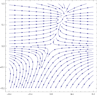
Figure 1: The RG flow (a) for $\tilde{\alpha}=-1,\tilde{\beta}=3$ and $b=0$. (b) Magnified one near origin.

We have checked how much these fixed points are dependent on the gauge parameter $b$. We show how $\tilde{G}_{*}$ changes for $-1<b<3$ in Fig. 2 (a) for $\tilde{\alpha}=-1,\tilde{\beta}=3$ and in (b) for $\tilde{\alpha}=1,\tilde{\beta}=3$. These parameters are chosen because we consider that it is natural to choose these of the order 1. We see that they both give qualitatively similar values and behaviors. In particular the absolute value is very small well below $b\sim 3$, so that this is certainly within the perturbative domain. Therefore, though our result is based on a one-loop calculation, we can expect that it correctly represents the features of the Wilsonian RG flow.

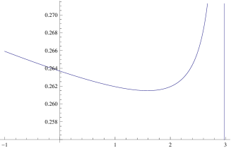
Figure 2: Gauge dependence of the nontrivial fixed point of $\tilde{G}_{*}$ (a) for $\tilde{\alpha}=-1,\tilde{\beta}=3$ and (b) for $\tilde{\alpha}=1,\tilde{\beta}=3$.

It is remarkable that the $b$-dependence disappears from the fixed point of the cosmological constant. As we saw in the preceding section, only $A_{1}$ and $B$ depend on $b$, but the combination $A_{1}+6B$ is precisely that appearing in the beta function of the dimensionless coupling (4.30), and hence that dependence drops out. We find that for the typical choice of $\tilde{\alpha}$ and $\tilde{\beta}$, the cosmological constant is positive and small; $0.057$ for $\tilde{\alpha}=-1$ and $\tilde{\beta}=3$, and 0.045 for $\tilde{\alpha}=1$ and $\tilde{\beta}=3$. The precise values may not be so important, but the fact that they are generally rather small may have some significance. Fig. 3 shows how the values of $\tilde{G}$ and $\tilde{\Lambda}$ change for $0<\tilde{\alpha}<3$ and $0<\tilde{\beta}<3$. This figure shows that the values are indeed small for a wide range of $\tilde{\alpha}$ and $\tilde{\beta}$ except near $8\tilde{\alpha}+3\tilde{\beta}=0$ and $\tilde{\beta}=0$, where these quantities are singular.

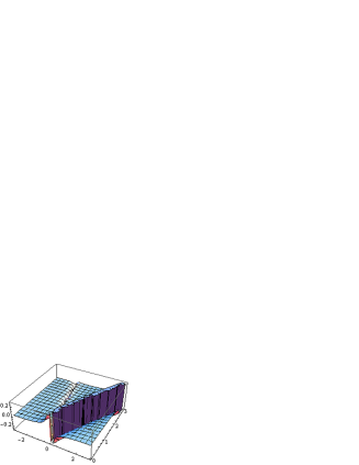
Figure 3: The fixed point values of (a) $\tilde{G}_{*}$ and (b) $\tilde{\Lambda}_{*}$ for $b=0$ as a function of $\tilde{\alpha}$ and $\tilde{\beta}$.

5.2 $\sigma=-1$

Let us now turn to the opposite sign for the Einstein term. Our RG equations (4.29) are well defined for the range $(\tilde{\beta}<0~{}\mbox{or}~{}\tilde{\beta}>1),~{}\mbox{and}~{}(8\tilde{\alpha}+3\tilde{\beta}<-1~{}\mbox{or}~{}8\tilde{\alpha}+3\tilde{\beta}>0).$ We shall be interested in the regions where unitary theories exist; $(\tilde{\alpha}\approx-\frac{3}{8}\tilde{\beta},\tilde{\beta}>0)$ or $(\tilde{\alpha}>0,\tilde{\beta}\approx 0)$. So the most interesting region is $(\tilde{\alpha}<0,\tilde{\beta}>1)$ and $(\tilde{\alpha}>0,\tilde{\beta}>0)$.

Here again there is the Gaussian fixed point which is attractive in the $\tilde{\Lambda}$ direction and repulsive in the $\tilde{G}$ direction. Another nontrivial fixed point in this case is given by

$$\tilde{G}_{*}=\frac{1}{B},~{}~{}\tilde{\Lambda}_{*}=\frac{A_{0}}{-A_{1}+6B}.$$ (5.2)

Let us see again the concrete values and the gauge dependence of the fixed point of the gravitational constant. For $\tilde{\alpha}=-1,\tilde{\beta}=3,b=0$, we find $\tilde{G}_{*}\sim-0.161$ and $\tilde{\Lambda}_{*}\sim 0.106$. The flow is shown in Fig. 4. We show how $\tilde{G}_{*}$ changes for $-1<b<3$ in Fig. 5 (a) for $\tilde{\alpha}=-1,\tilde{\beta}=3$ and in (b) for $\tilde{\alpha}=1,\tilde{\beta}=3$. We see that again they both give qualitatively similar values and behaviors. In particular the absolute value is again very small.

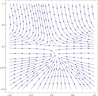
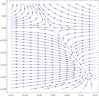
Figure 4: The flow is shown for $\tilde{\alpha}=-1,\tilde{\beta}=3$ and $b=0$. (b) is a magnified diagram.

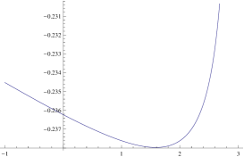
Figure 5: Gauge dependence of the concrete values of the nontrivial fixed point of $\tilde{G}_{*}$ (a) for $\tilde{\alpha}=-1,\tilde{\beta}=3$ and (b) for $\tilde{\alpha}=1,\tilde{\beta}=3$.

We note that the sign of the Newton constant changes from $\sigma=+1$ case and it takes negative value for typical values of $\tilde{\alpha}$ and $\tilde{\beta}$. Recall that in this case we took the negative sign for the Einstein term, but the fixed point of the gravitational constant takes negative values, resulting in positive Einstein term. Namely the Einstein term has positive coefficient at the fixed point even if we start with negative sign.

It is remarkable that the fixed point of the cosmological constant again does not depend on the gauge. We find that its values are $0.106$ for $\tilde{\alpha}=-1,\tilde{\beta}=3$ and $0.038$ for $\tilde{\alpha}=1,\tilde{\beta}=3$, again very small positive numbers. Fig. 6 shows how the values of $\tilde{G}$ and $\tilde{\Lambda}$ changes for $-3<\tilde{\alpha}<3$ and $0<\tilde{\beta}<3$.

Figure 6: The fixed point values of (a) $\tilde{G}_{*}$ and (b) $\tilde{\Lambda}_{*}$ for $b=0$ as a function of $\tilde{\alpha}$ and $\tilde{\beta}$.

6 Discussions and conclusions

In this paper we have studied the quantum effects of three-dimensional higher derivative gravity which has attracted much attention recently. In particular we have obtained the Wilsonian RG equations to study their fixed points. Though we did not attempt to derive those for the coefficients of the higher curvature terms because we cannot derive those for $\tilde{\alpha}$ and $\tilde{\beta}$ separately and also they become awfully complicated, we have some evidence that there is some fixed point for $\tilde{\alpha}$ and $\tilde{\beta}$. There are several conclusions we can draw even within this restriction. Assuming that $\tilde{\alpha}$ and $\tilde{\beta}$ have fixed points, we have found that there are ultraviolet fixed points for the gravitational and cosmological constants, one the usual Gaussian and the other nontrivial one for both signs of the Einstein term. This shows that this theory is asymptotically safe.

We have also found that the fixed point value of the gravitational constant is generically small, so that our one-loop discussion may well be justified. What is interesting is that if we take the negative sign for the Einstein term in the bare action, the gravitational constant has only a fixed point of negative values or zero, in the former case resulting in positive Einstein term. This is an interesting result which has not been explored in other approaches. It would be extremely interesting whether this happens also in four-dimensional gravity.

We have also shown that RG equations are singular for the parameters, $8\tilde{\alpha}+3\tilde{\beta}=0$ or $\tilde{\beta}=0$, corresponding to the new massive gravity or a special case of $f(R)$ gravity. Indeed, we see from Figs. 3 and 6 that $\tilde{G}_{*}$ and $\tilde{\Lambda}_{*}$ diverge there. If we look at the diagonalized action (3.18), we find that only the kinetic term for the transverse traceless mode is quadratic in the D’Alembertian but the rest are all linear, as can be seen from (3.19), and the limit is singular. This means that the new massive gravity and $f(R)$ gravity would not correspond to a fixed point in this class of theories. We would like to note that this result is one of the conclusions that are obtained within the approximation that the coefficients of the higher curvature terms $\tilde{\alpha}$ and $\tilde{\beta}$ are not subject to the flow, so strictly speaking there may be a possibility that the picture might be different in a larger space when these parameters are allowed to run.

Thus, though we did not attempt to evaluate the beta functions for $\tilde{\alpha}$ and $\tilde{\beta}$, it is quite interesting to examine whether the picture may change if we include those parameters in the RG analysis. For this purpose, we have to find a way to compute these for general backgrounds, not just for sphere, because we have to tell which is the contribution to $R^{2}$ and which is to $R_{\mu\nu}^{2}$. Probably the heat kernel method may be useful in such a study. We hope to return to this problem in the future.

References

• [1] K. S. Stelle, “Renormalization of Higher Derivative Quantum Gravity,” Phys. Rev.  D 16 (1977) 953.
• [2] E. A. Bergshoeff, O. Hohm and P. K. Townsend, “Massive Gravity in Three Dimensions,” Phys. Rev. Lett.  102 (2009) 201301 [arXiv:0901.1766 [hep-th]].
• [3] S. Deser, R. Jackiw and S. Templeton, “Topologically Massive Gauge Theories,” Annals Phys.  140 (1982) 372 [Erratum-ibid.  185 (1988) 406]
• [4] Y. Liu and Y. W. Sun, “On the Generalized Massive Gravity in AdS(3),” Phys. Rev.  D 79 (2009) 126001 [arXiv:0904.0403 [hep-th]].
• [5] M. Nakasone and I. Oda, “On Unitarity of Massive Gravity in Three Dimensions,” Prog. Theor. Phys.  121 (2009) 1389 [arXiv:0902.3531 [hep-th]].
• [6] S. Deser, “Ghost-free, finite, fourth order D=3 (alas) gravity,” Phys. Rev. Lett.  103 (2009) 101302 [arXiv:0904.4473 [hep-th]].
• [7] I. Gullu, T. C. Sisman and B. Tekin, “Canonical Structure of Higher Derivative Gravity in 3D,” Phys. Rev.  D 81 (2010) 104017 [arXiv:1002.3778 [hep-th]].
• [8] E. A. Bergshoeff, O. Hohm and P. K. Townsend, “More on Massive 3D Gravity,” Phys. Rev.  D 79 (2009) 124042 [arXiv:0905.1259 [hep-th]].
• [9] N. Ohta, “A Complete Classification of Higher Derivative Gravity in 3D and Criticality in 4D,” Class. Quant. Grav.  29 (2012) 015002 [arXiv:1109.4458 [hep-th]].
• [10] H. Nishino and S. Rajpoot, “(Curvature)**2-terms for supergravity in three dimension,” Phys. Lett.  B 639 (2006) 110 [arXiv:hep-th/0607241].
• [11] E. A. Bergshoeff, O. Hohm and P. K. Townsend, “Gravitons in Flatland,” arXiv:1007.4561 [hep-th].
• [12] K. Muneyuki and N. Ohta, “Unitarity versus Renormalizability of Higher Derivative Gravity in 3D,” Phys. Rev. D 85 (2012) 101501 [arXiv:1201.2058 [hep-th]].
• [13] S. Weinberg, “Ultraviolet Divergences In Quantum Theories Of Gravitation,” in Hawking, S.W., Israel, W.: General Relativity (Cambridge University Press, 1980), 790-831.
• [14] M. Reuter, “Nonperturbative evolution equation for quantum gravity,” Phys. Rev. D 57 (1998) 971 [hep-th/9605030].
• [15] A. Codello, R. Percacci and C. Rahmede, “Investigating the Ultraviolet Properties of Gravity with a Wilsonian Renormalization Group Equation,” Annals Phys.  324 (2009) 414 [arXiv:0805.2909 [hep-th]].
• [16] D. Benedetti, P. F. Machado and F. Saueressig, “Taming perturbative divergences in asymptotically safe gravity,” Nucl. Phys. B 824 (2010) 168 [arXiv:0902.4630 [hep-th]].
• [17] R. Percacci and E. Sezgin, “One Loop Beta Functions in Topologically Massive Gravity,” Class. Quant. Grav.  27 (2010) 155009 [arXiv:1002.2640 [hep-th]].
• [18] A. A. Bytsenko, L. N. Granda and S. D. Odintsov, “Exact renormalization group and running Newtonian coupling in higher derivative gravity,” JETP Lett.  65 (1997) 600 [hep-th/9705008].
• [19] O. Lauscher and M. Reuter, “Flow equation of quantum Einstein gravity in a higher derivative truncation,” Phys. Rev. D 66 (2002) 025026 [hep-th/0205062].
• [20] A. Codello and R. Percacci, “Fixed points of higher derivative gravity,” Phys. Rev. Lett.  97 (2006) 221301 [hep-th/0607128].
• [21] D. Benedetti, P. F. Machado and F. Saueressig, “Asymptotic safety in higher-derivative gravity,” Mod. Phys. Lett. A 24 (2009) 2233 [arXiv:0901.2984 [hep-th]].
• [22] A. E. Gumrukcuoglu and S. Mukohyama, “Horava-Lifshitz gravity with $\lambda\to\infty$,” Phys. Rev. D 83 (2011) 124033 [arXiv:1104.2087 [hep-th]].
• [23] P. A. Gonzalez, E. N. Saridakis and Y. Vasquez, “Circularly symmetric solutions in three-dimensional Teleparallel, f(T) and Maxwell-f(T) gravity,” JHEP 1207 (2012) 053 [arXiv:1110.4024 [gr-qc]].
• [24] D. F. Litim, “Optimized renormalization group flows,” Phys. Rev. D 64 (2001) 105007 [hep-th/0103195].