Metal-superconductor transition in two-dimensional electron systems with fractal-like mesoscopic disorder

Abstract

Motivated by recent experimental data on thin film superconductors and oxide interfaces we propose a random-resistor network apt to describe the occurrence of a metal-superconductor transition in a two-dimensional electron system with disorder on the mesoscopic scale. We explore the interplay between the statistical distribution of local critical temperatures and the occurrence of a lower-dimensional (e.g., fractal-like) structure of a superconducting cluster embedded in the two-dimensional network. The thermal evolution of the resistivity is determined by an exact calculation and, for comparison, a mean-field approach called effective medium theory (EMT). Our calculations reveal the relevance of the distribution of critical temperatures for clusters with low connectivity. In addition, we show that the presence of spatial correlations requires a modification of standard EMT to give qualitative agreement with the exact results.

I Introduction

Although two-dimensional (2D) electron systems have always been a topical subject in condensed matter physics, further renewed interest in this field has been triggered by the recent discovery of superconductivity at the metallic interface between two insulating oxide layers.reyren ; triscone ; espci In addition, experiments on certain thin conventional superconducting filmssacepe1 ; sacepe2 ; sacepe3 ; mondal reveal pseudogap effects, a phenomenon which could unveil new features of the superconducting transition in low-dimensional disordered systems.review_feigelman In the particularly interesting cases of homogeneously disordered superconducting titanium nitride or indium oxyde thin films, scanning tunneling spectroscopy data display inhomogeneities in the local density of states on mesoscopic spatial scales, clearly indicating the existence of an inhomogeneous superconducting state. Since tunneling experiments cannot directly access the 2D metallic layers at the oxide interfaces (although some attempts made on samples with very few top layers have detected interesting inhomogeneous texturessalluzzo ) magnetization and transport measurements are the only way to investigate these systems. Also in this case, evidences for an electronic phase separation have been found in LaAlO₃/SrTiO₃ layers.ariando Moreover, the sheet resistance curves $R_{\square}(T)$ near $T_{c}$, both in LaAlO₃/SrTiO₃ [triscone, ] and LaTiO₃/SrTiO₃ [espci, ] systems, show a peculiar feature of a marked tail on the low-temperature side.

Despite their differences, oxide interfaces and thin films share the common feature of a broad superconducting transition. In a previous work,CGBC we investigated the possible origin of this pronounced width and found that superconducting fluctuations (alone) cannot account for its occurrence, while a model of quenched mesoscopic disorder can well produce the observed broad transitions. In this previous work we also found that “tailish” features can occur in the resistivity curves when disorder has spatial correlations. Specifically, while uncorrelated disorder can generically account for the pronounced width of the metal-superconductor transition, tails only occur when disorder displays a correlated character or when it occurs on nearly one-dimensional subsets of the system. It is therefore important to understand how (correlated) disorder can act as to give rise to the tailish resistivity because this feature can be a signature of specific physical mechanisms at work in these systems. One natural possibility is that disorder correlations and/or nearly one-dimensional (or fractal) structures arise in the system from nanofractures, topological defects like crystal dislocations, steps, twinning domains, and so on. Another possibility is that low-dimensional superconducting subsets can spontaneously arise in the electronic gas even in the presence of a homogeneously distributed disorder. In particular, one should remember that, besides fluctuations of the energy gap $\Delta$, disorder can cause the localization of electrons, transforming an otherwise metallic system into an insulator. If the metal is also a superconductor then, at low temperatures, disorder can induce a superconductor-insulator transition.leema ; feigelman In this case, a theoretical proposal has been put forward, which predicts that superconductivity at high disorder is maintained by a fragile coherence within a small set of preformed Cooper pairs that are characterized by an anomalously large binding energy. Consequently, in the vicinity of the superconductor-insulator transition, both the insulator and the superconductor contain these preformed Cooper pairs that either localize, leading to an insulating state, or condense into a coherent state with a glassy behavior around the transition.leema ; feigelman ; ioffe ; feigelman10 The superconducting state then occurs on a small (possibly fractal) subset of the system, which forms in the electron gas around $T_{c}$.

To shed light on the physics of disordered low-dimensional superconductors, we carry out a systematic investigation of a 2D metallic system with quenched disorder represented by a random-resistor network (RRN). As in our previous work of Ref. [CGBC, ], the resistors represent mesoscopic metallic islands where superconductivity occurs at a local critical temperature $T_{c}$. The superconducting regions are assumed to be large enough to have a fully established local coherence and to make the charging effects negligible. As a consequence, a mutual phase coherence immediately establishes between two neighboring superconducting islands, as soon as both have become superconducting. This clearly distinguishes our framework from the case of granular superconductors, where the grains have usually nanoscopic sizes of the order of the coherence length of the pure system. In this way we disregard phase-fluctuation effects in order to unambiguously identify the effects of disorder (and of its specific character). In particular, to understand the effects of spatial correlations, we investigate here the effects of two fractal-like distributions of the disordered resistors. In this way, while completely disregarding the underlying mechanisms leading to such correlated disordered structures, we focus on their phenomenology.

The paper is structured as follows. In Section II we introduce the generic aspects of our model, while in Section III we report the results of our numerical calculations for various kinds of fractal structures and of disorder distributions. Section IV contains a discussion of the results and our concluding remarks.

II The Random-Resistor Model and Effective Medium Theory

In a previous workCGBC we considered a model of a 2D electron gas with mesoscopic defects as a square lattice whose bonds are assigned a random resistivity $\rho_{i}$. More precisely, each bond is assigned a local superconducting transition temperature $T_{c}^{(i)}$, extracted from a given distribution $\mathcal{W}(T_{c})$, and the resistivity of the bond is written as $\rho_{i}=\rho_{0}\theta(T-T_{c}^{(i)})$, with the same high-temperature value $\rho_{0}$ on all bonds, $\theta(x)$ being the Heaviside step function. By decreasing the temperature $T$, more and more bonds become superconducting, and global superconductivity establishes as soon as a percolating superconducting path is formed in the system.

The simplest description of a RRN is provided by the effective medium theoryeffectivemedium ; kirkpatrick (EMT), which is a mean-field treatment replacing the random resistors $\rho_{i}$ with an effective medium resistivity $\rho_{em}$ such that

$$\sum_{i}\frac{\rho_{i}-\rho_{em}}{\alpha\rho_{i}+\rho_{em}}=0,$$ (1)

where the parameter $\alpha$ is related to the connectivity of the network. For a cubic network in $D$ spatial dimensions, $\alpha=D-1$.

In the previous work of Ref. [CGBC, ] (to which we refer the reader for further detail), we used EMT as a benchmark and compared $\rho_{em}$ with the exact numerical determination of the resistance of the RRN, obtained solving the Kirchhoff equations for the network in the presence of a difference of potential $V$ between two opposite sides of a $N\times N$ square lattice. Once the current $I(T)$ flowing through the network at a temperature $T$ is obtained, the resistance is found as $R(T)=V/I(T)$. We showed that EMT provides a very good description of the temperature dependence of the resistivity, independently of the distribution of $T_{c}$, provided disorder is spatially uncorrelated.

The solution of Eq. (1), specialized to our case, readsCGBC ; kirkpatrick

$$\rho_{em}(T)=(1+\alpha)\rho_{0}\theta(T-T_{\alpha})\int_{T_{\alpha}}^{T}dT_{c}\,\mathcal{W}(T_{c}).$$ (2)

Here, $T_{\alpha}$ is the critical temperature of the effective medium and is determined by the equation

$$w_{s}(T_{\alpha})\equiv\int_{T_{\alpha}}^{+\infty}dT_{c}\,\mathcal{W}(T_{c})=\frac{1}{1+\alpha},$$ (3)

where $w_{s}(T)\equiv\int_{T}^{+\infty}dT_{c}\,\mathcal{W}(T_{c})$ is the statistical weight of the superconducting bonds at a temperature $T$, measuring the frequency of occurrence of bonds with $T_{c}>T$. From Eq. (2) it is readily seen that $\rho_{em}\to\rho_{0}$ for $T\to\infty$ and $\rho_{em}(T_{\alpha})=0$.

In the present paper we consider a model in which the superconducting bonds only form a spatially correlated subset of the whole system. This subset provides a “skeleton” network of bonds which become superconducting below a random local $T_{c}^{(i)}$, while the embedding system is a metal with temperature-independent resistive bonds. We shall explore the joint effects of the connectivity of the network and of the statistical distribution of the local critical temperature $\mathcal{W}(T_{c})$. We shall mainly rely on the exact numerical solution of the Kirchhoff equations, but shall refer to the EMT results to provide an interpretation to the outcomes of our calculations. When dealing with EMT, the presence of spatial correlations requires the introduction of an effective connectivity $\alpha$, different from the standard connectivity.

III Effects of fractal-like disordered structures

III.1 The general framework

To systematically investigate the effects of correlated disorder, we consider the occurrence of a cluster where the zero-resistance state is carried by only a minor set of superconducting regions, reducing the effective dimension of the 2D electron gas. We disregard the physical origin (classical, as due to mechanical stresses, non-uniform growth and so on, or quantum-mechanical, as - for example - associated with the occurrence of coherence on a thin cluster of Cooper pairs near the superconductor-insulator transition) of this low-dimensional superconducting “skeleton” and we translate it into the framework of the RRN. Specifically, we consider a RRN on which fractal-like structures are superimposed, i.e., clusters exhibiting strong spatial correlations and scale invariance (although the scale invariance is limited, once the structure is implemented on a finite - e.g., $100\times 100$ - lattice). Each bond of these spatially correlated clusters is given a critical temperature extracted from a probability distribution $\mathcal{W}(T_{c})$, while the bonds not belonging to the “fractal” cluster have fixed resistances $\rho_{0}$ (throughout the paper we take $\rho_{0}=1$). By varying the geometry of the clusters, as well as the probability distribution, the influence of these two aspects on the temperature dependence of the resistivity is studied. Note that in this approach the spatial distribution of superconducting bonds is considered to be independent from the probability distribution of the critical temperatures. This is a simplifying assumption allowing for a more general and systematic analysis of the separate effects of geometry and of statistical distribution. This assumption should of course be dropped whenever the physical mechanisms selecting the “fractal” superconducting cluster also determine its $T_{c}$ distribution.

It is worth pointing out that in the previously considered models of uniform uncorrelated disorderCGBC , global superconductivity occurred as a true percolative phenomenon: Upon lowering the temperature, more and more bonds became superconducting until a percolative cluster of superconducting bonds was reached. The geometrical support and the general features of this transition were typical of the percolation transition. On the other hand, in the present model the geometric support of bonds which can become superconducting is provided by a predetermined fractal-like subset of the network. When $T$ is lowered, more and more bonds on this fractal support become superconducting and global superconductivity only occurs when a percolating path through the whole system is formed inside the subset. In this case, for instance, the fractal dimension of the superconducting support is not due to pure percolation, but it clearly depends on the dimensionality of the supporting fractal-like subset. This “percolation inside a fractal” is what gives rise to global superconductivity in the present model.

In order to cover a wide range of possible $T_{c}$ distributions we choose the two extreme cases of Gaussian and Cauchy statistics. The choice is motivated by their different asymptotic behavior: While the first has small tails and well defined momenta at all orders, the second is characterized by strong tails causing all momenta except the mean to diverge. We take a Gaussian defined by the mean value $\mu_{1}$ and variance $\sigma$,

$$\mathcal{W}(T_{c})=\frac{1}{\sqrt{2\pi}\sigma}{\mathrm{e}}^{-(T_{c}-\mu_{1})^{2}/2\sigma^{2}}$$ (4)

and a Cauchy (i.e., Lorentzian) distribution defined by the mean value $\mu_{2}$ and the width $\gamma$,

$$\mathcal{W}(T_{c})=\frac{\gamma}{\pi[\gamma^{2}+(T_{c}-\mu_{2})^{2}]}$$ (5)

Throughout the paper the same parameters $\mu_{1}=\mu_{2}=1$, $\sigma=0.1$ and $\gamma=0.08$ will be adopted. The parameters $\sigma$ and $\gamma$ are chosen so that the resistivity curves obtained with the Gaussian and Cauchy distribution have the same slopes close to the transition when space correlations are absent (Fig. 1).

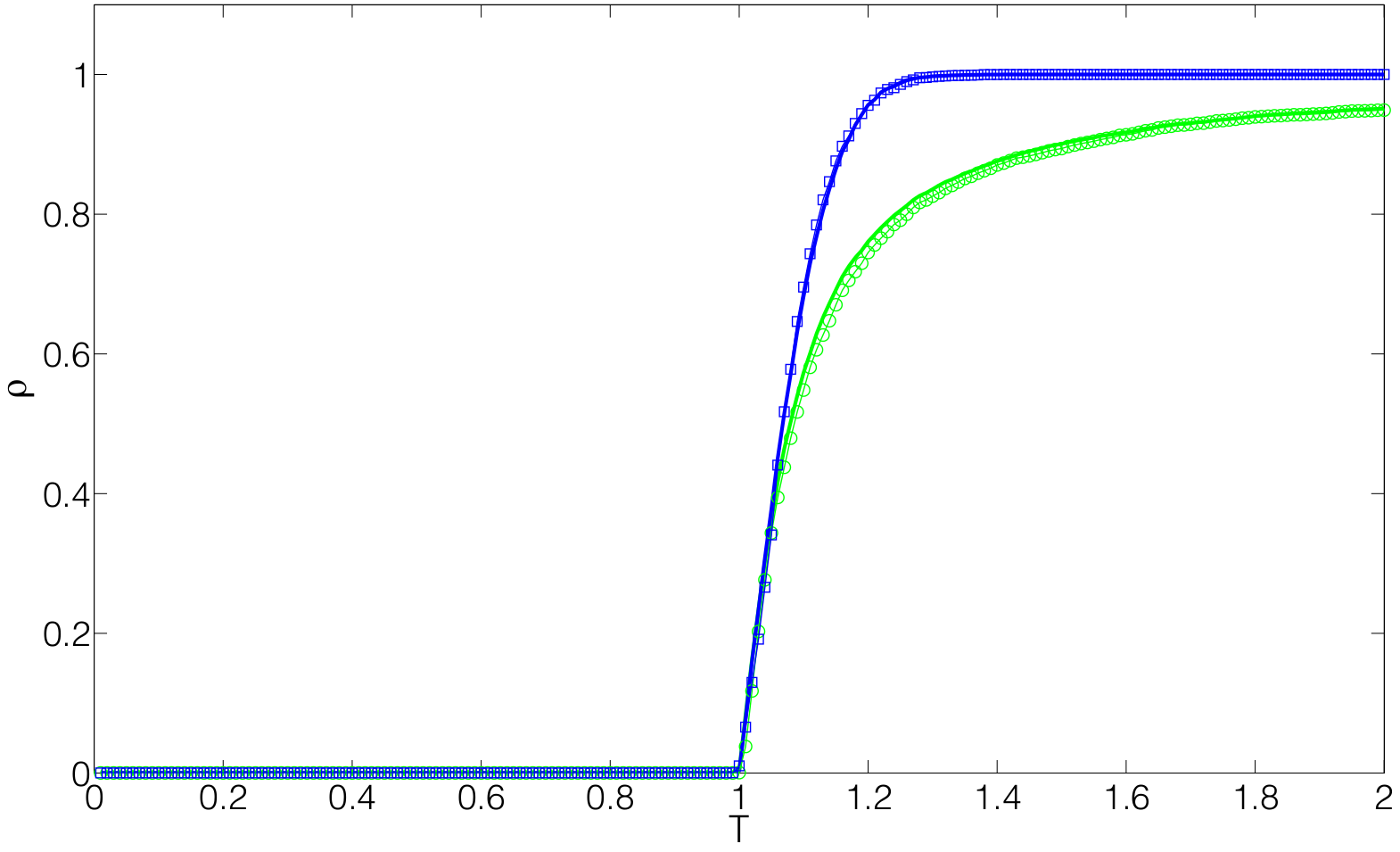
Figure 1: (Color online) Resistance curves of the uniform cluster. The blue curves correspond to a Gaussian distribution with $\mu=1,\sigma=0.1$ and the green to a Cauchy distribution with $\mu=1,\gamma=0.08$. The markers report the thermal evolution of the resistance obtained through the exact numerical calculations and the full lines the EMT solution.

As recalled in Sec. II, one of the findings of Ref. [CGBC, ] was that in the absence of space correlations EMT performs remarkably well in reproducing the exact results of the RRN, irrespective of the specific $T_{c}$ distribution. As an illustration, we report in Fig. 1 the resistivity curves of a uniform system obtained with the distributions here considered: The Gaussian (blue curves) and the Cauchy distribution (green curves). One notices that the resistance curves obtained with EMT match very well the exact numerical solutions. Thus, in the absence of correlations, EMT provides a useful tool to investigate the $\rho(T)$ dependence. In particular, the theory states that the resistivity of a RRN vanishes as soon as the weight of superconducting bonds $w_{s}$ exceeds $1/(1+\alpha)$, where $\alpha$ is the connectivity of the system. In the present case of a uniform two dimensional lattice, $\alpha=1$ and the percolation threshold at the transition yields $w_{s}=1/2$. Referring to the resistance curves in Fig. 1, one notices that the critical temperature of the system is $T_{\alpha}=1$, coinciding with the mean value of the (symmetric) distributions where half of the bonds have become superconducting. Thus, we correctly reproduce the predicted value of $w_{s}=1/2$. At high temperature, the heavier tail of the Cauchy distribution results in a greater number of bonds with switched-off resistance. The resistivity for the Cauchy distribution remains smaller until the temperature $T_{\alpha}=1$ is reached where $w^{\mathrm{C}}_{s}=w^{\mathrm{G}}_{s}=1/2$, the superscripts $C,G$ referring henceforth to the Cauchy and Gaussian distribution, respectively.

To give a quantitative picture of the resistivity close to $T_{\alpha}$ one can take the derivative of Eq. (2) defined in the framework of EMT:

$$\rho^{\prime}_{em}(T)=(1+\alpha)\rho_{0}\mathcal{W}(T_{c}=T),$$ (6)

for $T\geq T_{\alpha}$, which shows that the slope of the resistivity is proportional to the value of the distribution at equal temperatures. Combining this equation with the previous result $w_{s}(T_{\alpha})=1/2$, where the distribution has a maximum, one concludes that it is impossible to obtain “tails” in the present case. In fact, due to the bell-shape of the distributions the slope of the $\rho(T)$ is maximal at the mean value and thus also at the critical temperature of the system. In the same line of reasoning, one realizes that a tailish behavior can be obtained even for a spatially uncorrelated distribution, in the very specific case of a symmetric bimodal distribution of $T_{c}$’s (see Ref. [CGBC, ]). Here, we disregard this possibility and focus instead on the issue of space correlations.

III.2 Diffusion Limited Aggregation

The first fractal-like cluster we implement is obtained through a simple growth process, generated by Brownian motion and known as diffusion limited aggregation (DLA). Its construction is quite simple: A particle is released at the left edge of a 2D lattice and let diffuse to the right. More precisely, the particle moves one bond to the right and then with equal probability one bond up or down. This procedure is iterated until the particle stops, as soon as it reaches the top, bottom or right edge, where it sticks. Then, other particles are launched in sequence and halted either when reaching one of the three edges or a bond already occupied by one of the previously diffused particles. The cluster obtained in a $250\times 250$ square lattice after diffusing $50000$ particles is defined by the bonds where the particles sticked. Due to a saturation at the left edge, the total number of superconducting bonds only amounts to about $25000$. Once this large cluster is obtained, we select a $100\times 100$ sub-lattice as shown in Fig. 2 and perform the calculations for this smaller cluster. In this way, we try to model a more physical case where the fractal covers the whole sample. So henceforth, we consider a $100\times 100$ lattice, where only bonds belonging to the cluster are assigned a critical temperature $T_{c}$. The other bonds form a resistive background and are assigned the resistivity $\rho_{0}$ at all temperatures.

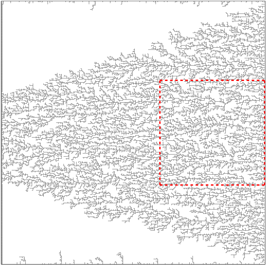
Figure 2: Spatial distribution of superconducting bonds obtained through diffusion limited aggregation. The red square indicates the $100\times 100$ lattice which is used for the calculations.

Fig. 3 reports the resistance curves calculated on the $100\times 100$ DLA cluster. We remark that for $T\gtrsim 1$ the curves for the Gaussian and Cauchy distribution are rather similar. Lowering the temperature, the system starts to exhibit a stronger dependence on the specific statistics. In the Gaussian case, a percolating path is already formed around $T_{\alpha}=0.78$, whereas for the Cauchy distribution one has to go as low as $T_{\alpha}=0.33$ for the system to become fully superconducting. Examining the formation of the superconducting cluster, one finds that at $T_{\alpha}$, the fraction of superconducting bonds are $w_{s}^{G}=0.99$ and $w_{s}^{C}=0.97$ respectively. So practically all the bonds have to be superconducting in order for the phase transition to occur.

The reason for this strong condition lies in the very small set of percolating paths, i.e., the effective connectivity of the cluster is very close to zero. In other words, the cluster has a rather marked one-dimensional character and few missing superconducting bonds are enough to prevent the system from percolating. To give a quantitative estimate of the effective connectivity of the cluster we define the following measure (inspired by Eq. (3) defined in the EMT framework),

$$\alpha^{eff}=\frac{1}{w_{s}(T_{\alpha})}-1.$$ (7)

For instance, comparing $w_{s}^{U}(T_{\alpha})=0.5$ and $w_{s}^{G,DLA}(T_{\alpha})=0.99$, where the superscripts $U$ and $DLA$ refer to the case of a uniform and DLA superconducting cluster, respectively, one realizes that the statistical weight of the superconducting bonds clearly depends on the geometry of the cluster and, in particular close to the critical temperature $T_{\alpha}$, on its effective connectivity. In addition, we shall show below that taking $\alpha^{eff}_{DLA}=1/0.99-1=0.01$ the EMT restricted to the cluster produces $\rho(T)$ curves close to the exact results. Therefore, even though space correlations do not enter explicitly, equation (7) still provides a good estimate for an effective connectivity, once the relevant space correlations are accounted for by restricting EMT to the cluster. A second effect of the small set of percolation paths is a strong dependence on the specific realization of the distribution. Since the number of bonds in the percolating cluster is at most of order $N^{D}$ (where $D$ is the fractal dimension of the cluster), two different realizations of the same distribution might be quite different. This effect is particularly severe for the Cauchy distribution, which has larger deviations from the mean. Since the Gaussian distribution, having small deviations from the mean, produces a superconducting cluster with an effective connectivity $\alpha_{DLA}^{eff}=0.01$, we assume this value as representative of the appropriate connectivity of the underlying DLA cluster. On the other hand, the realization of the Cauchy distribution of critical temperatures on the cluster in Fig. 2 is such that a percolating path forms at finite temperature but, calculations of $\rho(T)$ for different realizations of $\mathcal{W}(T_{c})$ show that on average the phase transition does not occur. This result can be understood by noticing that the Cauchy distribution has rather wide tails so that $w_{s}^{C}(T\leq 0)\approx 0.025$. Thus the fraction of bonds, which never become superconducting is substantial and, owing to the low connectivity of the DLA cluster (requiring $w^{DLA}_{s}=0.99$), it may well happen that non-superconducting bonds prevent full percolation to be established down to zero temperature.

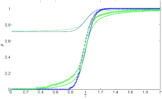
Figure 3: (Color online) Resistance curves of diffusion limited aggregation cluster. The blue curves correspond to a Gaussian distribution with $\mu=1,\sigma=0.1$ and the green to a Cauchy distribution with $\mu=1,\gamma=0.08$. The markers report the thermal evolution of the resistance obtained by exact numerical calculations, the dashed lines by EMT on the system and the full lines by EMT on the cluster.

This effect makes it quite apparent that on correlated clusters, the low values of connectivity (like $\alpha^{eff}_{DLA}=0.01$) renders the system very sensitive to the statistics of the critical temperatures.

Fig. 3 also shows that the EMT, when applied to the whole RRN (which is formed both by the fractal-like cluster and its complementary background), clearly misses the correct temperature dependence of the resistivity. According to its construction, outlined in Sec. II, this mean-field-like theory neglects all spatial correlations and this discrepancy is expected. In addition, we remark that the decrease of $\rho$ with $T$ is a finite-size effect: As soon as we introduce spatial correlations, the cluster dimension $D$ becomes smaller than $2$, and the statistical weight of superconducting bonds is smaller (or equal) than $N^{D}/N^{2}$ which tends to zero for $N\rightarrow\infty$.

One can try to circumvent the shortcomings of EMT by evaluating it on the bonds belonging to the DLA cluster only. With this adjustment, the relevant space correlations are effectively incorporated and EMT with the effective connectivity reproduces quite accurately the main features of the exact solution: The regular behavior for $T>\mu$ and the stronger dependence on the distribution at low temperatures, due to the cluster’s low connectivity. However, there is an overall shift from the restricted EMT solution with respect to the exact calculation. At high temperatures, where only very few bonds have become superconducting, it is not favorable to force the current to flow through many resistive bonds simply to reach a few superconducting bonds. Therefore, the current still flows through the system in parallel (only locally perturbed by the few superconducting bonds present). By decreasing the temperature the superconducting cluster increases and consequently, also the amount of current going through it. Close to the transition the shift then nearly vanishes because the resistive background ceases to play an important role. More precisely, the current is essentially carried by one or a few large quasi-percolating paths, which only need few resistors to switch off in order to fully percolate. For these paths, it is immaterial whether they are embedded in a two-dimensional (markers in Fig. 3) or simply a quasi one-dimensional system (full lines in Fig. 3).

III.3 Symmetrized Random Walk

The topology of the DLA cluster considered in the previous section is characterized by few backbones (forming connected paths between the two vertical edges of the lattice) and many dangling branches. Now, we explore a different situation in which the fractal-like geometry does not contain any dangling branches.

We modify the construction scheme of the DLA in the following way: Instead of keeping only the final position of the diffused particles, their entire trajectory is incorporated into the cluster. In addition, the particles are free to cross the paths of previously diffused particles. Launching $50$ particles from each of the four edges and letting them diffuse perpendicular to the initial edge, a cluster of the form shown in Fig. 4 is obtained.

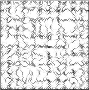
Figure 4: Spatial distribution of superconducting bonds obtained through a symmetrized random walk on a $100\times 100$ lattice.

As it was the case for the DLA, the resistance curves of the symmetrized random walk (SRW) shown in Fig. 5 are very similar for $T\gtrsim 0.9$, the small difference originating simply from the difference in the distributions. Looking at the superconducting cluster formed at $T=0.9$, one finds that the weights of superconducting bonds are $w_{s}^{G}=0.84$ and $w_{s}^{C}=0.79$, respectively. Interestingly, this difference has no effect on the resistivity. In fact, at this temperature, the size of connected superconducting regions is of the order of $10$ bonds for both distributions. In this regime, having a few superconducting bonds more or less does not produce a noticeable difference in the resistivity.

This behavior clearly changes as one approaches the transition temperature. For $T$ slightly larger than $T_{\alpha}$ the current is carried by long-range superconducting regions which lack only few bonds to fully percolate. Inspection of the superconducting cluster growth reveals that the percolation threshold is reached as soon as $w_{s}^{G}(T_{\alpha}^{G})=0.92$ and $w_{s}^{C}(T_{\alpha}^{C})=0.90$. The closeness of these two values is again an indication that the threshold weight $w_{s}(T_{\alpha})$ only depends on the “geometry” (i.e. its effective connectivity) of the underlying cluster and not on the specific $T_{c}$ distribution. While the threshold is reached at $T_{\alpha}^{G}=0.86$ in the first case, the heavy tail of the Cauchy distribution obliges the system to go as low as $T_{\alpha}^{C}=0.76$ in the second case.

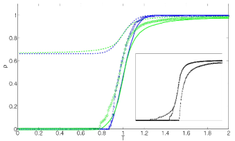
Figure 5: (Color online) Main panel: Resistance curves of symmetrized random walk cluster. The blue curves correspond to a Gaussian distribution with $\mu=1,\sigma=0.1$ and the green to a Cauchy distribution with $\mu=1,\gamma=0.08$. The markers report the thermal evolution of the resistance obtained by exact numerical calculations, the dashed lines by EMT on the system and the full lines by EMT on the cluster. The inset shows a comparison of the exact resistivity curves obtained with a Cauchy distribution ($\mu=1,\gamma=0.08$) for the uniform (circles), the DLA (pluses) and the SRW (squares) cluster, respectively.

These considerations on $w_{s}^{U}$, $w_{s}^{DLA}$ and $w_{s}^{SRW}$ suggest that the high-temperature behavior is mainly determined by the dimensionality of the cluster. In fact, coarse-graining analysis using the box-counting methodHalsey shown in Fig. 6 reveals that the dimension of the clusters is $D^{DLA}\approx D^{SRW}\approx 1.8$. This is reflected in the congruence of $\rho^{DLA}(T)$ and $\rho^{SRW}(T)$ for $T>0.9$, as well as in their leftward shift with respect to $\rho^{U}(T)$ (with $D^{U}=2$), as is shown in the inset of Fig. 5.

In contrast, the calculation of the connectivity at the transition point reveals that $\alpha^{eff}_{SRW}\approx 0.1$, which corresponds to a nearly one-dimensional cluster. So, despite its 2D appearance, the low-temperature region, being more sensitive to the effective connectivity than to the dimensionality, behaves as quasi-one-dimensional. As far as the comparison between the EMT and the numerical exact results is concerned, the conclusions are analogous to the discussion given for the DLA cluster.

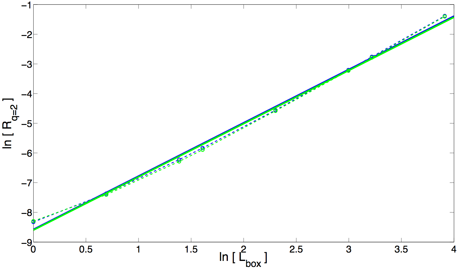
Figure 6: (Color online) Determination of fractal dimension using the box-counting method: The lattice is subdivided into $N_{box}=(N/L_{box})^{2}$ boxes of size $A_{box}=L_{box}\times L_{box}$. For each box $k$, we calculate the ratio $\mu_{k}=N^{k}_{bond}/N_{c}$, between the number of bonds belonging to the portion of the cluster inside this box $N^{k}_{bond}$ and the total number of bonds belonging to the cluster $N_{c}$. The quantity $R_{q}=\sum_{k=1}^{N_{box}}\mu_{k}^{q}$ is then related to the box size according to $R_{q}=L_{box}^{D(q-1)}$, where $D$ is the fractal dimension. The figure shows a log-log plot with $L_{box}$ varying from $1$ to $N/2$ (circles). The full lines are linear regressions of $\text{ln}\,R_{q=2}\propto D\,\text{ln}\,L_{box}$; the DLA cluster (green curve) and the SRW cluster (blue curve) have both slope $D=1.8$.

To develop a quantitative understanding of $\rho(T)$ close to the transition, we turn to an analytic approach based on a coarse-grained picture of the cluster. We consider the random walk cluster as a uniform system made up by large conducting segments containing $M\gg 1$ bonds. In the framework of EMT the percolation threshold is reached when $1/2$ of the segments are superconducting. One can reformulate the condition in terms of the single bonds; in order for a large segment to become superconducting, all its single bonds have to be superconducting, i.e.,

$$p^{M}=1/2$$ (8)

where $p$ is the probability for a single bond to be superconducting. Close to the global critical point, the resistivity can be approximated by

$$\rho(T\gtrsim T_{c})=C\rho_{0}\left(\frac{1}{2}-p^{M}\right),$$ (9)

with $C>0$. The purpose of the model is to analyze the possible occurrence of a tail in the resistivity curve, i.e., the behavior of the slope of $\rho(T)$ at $T\approx T_{c}$:

$$\frac{d\rho}{dT}\Big{|}_{T\approx T_{c}} = -Mp^{M-1}p^{\prime}$$ (10)

where $C\rho_{0}$ was set to $1$ for simplicity and $p^{\prime}=dp/dT$. Since $T\approx T_{c}$ and $M\gg 1$ the following approximations can be made,

$$p^{M} \approx \frac{1}{2}$$ (11)

$$p \approx \exp\left[-\frac{1}{M}\ln(2)\right]\approx 1-\frac{1}{M}\ln(2)$$ (12)

$$\Rightarrow M=\frac{\ln(2)}{1-p}$$ (13)

Inserting the two expressions into Eq. 10, we get an expression for the derivative of the resistivity as a function of the single bond probability close to the critical point,

$$\frac{d\rho}{dT}\Big{|}_{T\approx T_{c}} = -\frac{1}{2}\ln(2)\frac{p^{\prime}}{p(1-p)}$$ (14)

$$\approx -\frac{1}{2}\ln(2)\frac{p^{\prime}}{1-p}$$ (15)

$$= \frac{1}{2}\ln(2)\frac{\mathcal{W}(T_{c})}{1-\int_{T_{c}}^{\infty}\mathcal{W}(\tilde{T}_{c})d\tilde{T}_{c}}.$$ (16)

In terms of the distribution the condition $p\approx 1$ (see Eq. (14)) means that the leading behavior is obtained taking the limit $\mathcal{W}(T_{c}\rightarrow-\infty)$ (or, more precisely, $\mu-T_{c}\gg\sigma,\gamma$; we point out that the critical temperature stays finite). This implies that the slope of the resistivity is proportional to the ratio of two small numbers. For the Gaussian distribution, the ratio is

$$\frac{\mathcal{W}(T_{c})}{1-\int_{T_{c}}^{\infty}\mathcal{W}(\tilde{T}_{c})d\tilde{T}_{c}}\approx\frac{\frac{1}{\sqrt{2\pi}\sigma}{\mathrm{e}}^{-x^{2}}}{1-\left(1-\frac{{\mathrm{e}}^{-x^{2}}}{\sqrt{\pi}|x|}\right)}$$

$$=\frac{|x|}{\sqrt{2}\sigma}\approx\frac{|T_{c}-\mu_{1}|}{2\sigma^{2}},$$ (17)

where the short-hand notation $x=(T_{c}-\mu_{1})/\sqrt{2}\sigma$ was used. For the Cauchy distribution, the ratio is

$$\frac{\mathcal{W}(T_{c})}{1-\int_{T_{c}}^{\infty}\mathcal{W}(\tilde{T}_{c})d\tilde{T}_{c}}\approx\frac{\frac{\gamma}{\pi[\gamma^{2}+(T_{c}-\mu_{2})^{2}]}}{1-\left(1-\frac{\gamma}{\pi T_{c}}\right)}$$

$$\approx\frac{1}{|T_{c}-\mu_{2}|}.$$ (18)

One observes that the slope for the Gaussian distribution depends linearly on the deviation from the critical temperature, while in the case of the Cauchy distribution the dependence is inversely proportional. The evaluation of the expressions (III.3) and (III.3) with the results of the SRW yields $\rho^{\prime}(T_{c}^{G})\approx\rho^{\prime}(T_{c}^{C})\approx 0.15$, which is smaller than the exact results given in Fig. 5. The reason for this mismatch lies in the assumption $M\gg 1$, while in the present case $M\approx 5$ . Nevertheless, the calculations highlight the strong influence of the distribution for low-dimensional structures with $M\gg 1$.

To investigate the SRW and illustrate the analytic approach presented above, we briefly consider a cluster obtained through coarse graining. The cluster contains every fifth column and fifth row of the original network. In this way, one obtains a uniform grid equivalent to the uniform case of a $N/5\times N/5$ lattice where each bond is made up by $5$ bonds of the original network.

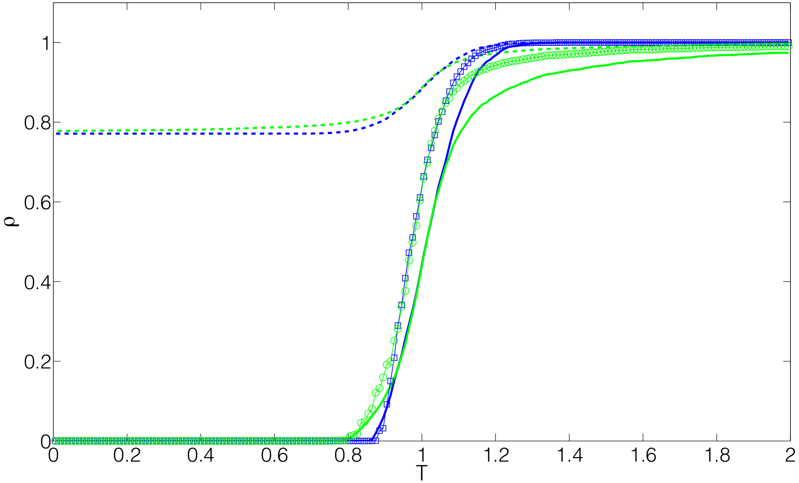
Figure 7: (Color online) Resistance curves of coarse grained cluster. The blue curves correspond to a Gaussian distribution with $\mu=1,\sigma=0.1$ and the green to a Cauchy distribution with $\mu=1,\gamma=0.08$. The markers report the thermal evolution of the resistance obtained by exact numerical calculations, the dashed lines by EMT on the system and the full lines by EMT restricted to the cluster.

Comparison of Fig. 7 and Fig. 5 reveals a marked resemblance between the $\rho(T)$ curves for the random walk and the coarse grained cluster. This shows that the regular coarse-grained cluster indeed captures the main features of the strongly disordered SRW cluster.

IV Conclusions

Our analysis is purely phenomenological in character: We embed a given fractal-like structure in a purely metallic environment, we impose a given $T_{c}$ distribution on it, and then we calculate the resulting resistivity curve. While, as we already mentioned, this approach lacks any (possible, but not mandatory) microscopic connection between the geometrical and the $T_{c}$ distribution, we separately access the distinct effects of these two ingredients.

As a first result, we would like to point out that the geometrically correlated character of the superconducting clusters considered here greatly degrades the performance of the EMT mean-field-like approach. According to our experience in spatially uncorrelated disorderCGBC , this failure has nothing to do with the strength of disorder or the relative density of the superconducting and the non-superconducting bonds, but is a mere result of space correlations. On the other hand, we showed that it is possible to find a good qualitative agreement by restricting EMT to the cluster. In this case, one needs to introduce an effective connectivity (see Eq. (7)).

Calculating the standard (local) connectivity given by $\alpha=\langle z\rangle/2-1$, where $\langle z\rangle$ is the average number of nearest neighbors, we obtain $\alpha_{DLA}=0.38$ and $\alpha_{SRW}=0.15$. The comparison with $\alpha^{eff}_{DLA}=0.01$ and $\alpha^{eff}_{SRW}=0.1$ reveals that the effective connectivity is very different from the locally defined connectivity. This is quite natural since we are considering transport phenomena, which are ruled by paths connecting distant regions of the system. In other words, the presence of regions with large internal connectivity, is rather immaterial for transport if this regions are weakly connected to one another.

We also find that the effective connectivity is an intrinsic property of the cluster and is independent of the $T_{c}$ distribution. This result is quite natural because upon reducing $T$, the $T_{c}$ distribution only determines how “fast” the resistances are switched off. However, this is irrelevant as far as the amount of superconducting bonds needed to percolate is concerned.

The main outcome of our analysis is that the effects of space correlations render the superconducting transition strongly dependent on the disorder distribution, and in particular on its low-temperature asymptotics. This is not surprising: As soon as percolation happens through a quasi one-dimensional path, the system needs to explore (almost) the entire $T_{c}$ distribution, and thus becomes very sensitive to its low-temperature part. This effect can be made particularly clear within the analytic approach of Sec. III.3, where the slope of the resistivity at $T_{c}$ was shown to depend in inverse ways on the distance of $T_{c}$ from the mean of the Cauchy or Gaussian distribution.

After the detailed analysis of the various effects of space correlations and $T_{c}$ statistics we come back to the initial question of whether and which of these aspects is relevant in explaining the tailish behavior of $\rho(T)$ in oxide interfaces. Based on the above results a possible ingredient is indeed a fractal-like structure of superconducting bonds. Due to its high dimensionality (i.e. larger than a purely one-dimensional cluster), the cluster consists of enough superconducting bonds to cause a linear decrease of the resistance with a relatively high slope. Close to the percolation threshold, however, the crucial property determining the shape of the transition is not the dimensionality but the effective connectivity. There, the quasi-one-dimensional behavior of the DLA and SRW clusters results in a more or less pronounced tail of $\rho(T\gtrsim T_{\alpha})$. The shape of the tail is then controlled (to some extent) by the low-temperature asymptotics of the distribution.

Our analysis and approach are therefore a useful tool to explore the physical mechanisms at work in the superconducting oxide interfaces, where a precise fitting of the resistance curves provides indications on both the intra-grain mechanisms leading to a local $T_{c}$ and to the inter-grain connection ruling the establishing of the global superconducting state via the percolative “chaining” of superconducting regions on the fractal support (see Sec. III.1 for the specific meaning of the word “percolative” in the present model). The intragrain superconductivity manifests itself in the high-temperature region of the resistivity, where the restivity starts to bend down when isolated superconducting regions are created. In this case the $T_{c}$ distribution and the relation between its width and the high temperature resistivity might provide informations on the intra-grain pair formation (Cooper pairs in the presence of quenched impurities,finkelstein disordered bosonic preformed pairs,fisher glassy superconducting transition.ioffe ; feigelman10 ) On the other hand, near the global $T_{c}$, the second percolative phenomenon is ruled by the geometric character (in particular by the effective connectivity) of the superconducting cluster, and might be informative about the origin of the inhomogenous metal-superconductor structure with coexisting metallic and superconducting islands.

Acknowledgments. We are indebted with N. Bergeal, J. Biscaras, C. di Castro, B. Leridon, J. Lesueur, and J. Lorenzana, for interesting discussions and useful comments. S.C., C. C., and M.G. acknowledge financial support from “University Research Project” of the “Sapienza” University n. C26A115HTN.

References

- (1) N. Reyren, S. Thiel, A. D. Caviglia, L. Fitting Kourkoutis, G. Hammerl, C. Richter, C. W. Schneider, T. Kopp, A.-S. R etschi, D. Jaccard, M. Gabay, D. A. Muller, J.-M. Triscone, and J. Mannhart, Science 317, 1196 (2007).
- (2) A. D. Caviglia, et al., Nature (London) 456, 624 (2008).
- (3) J. Biscaras, N. Bergeal, A. Kushwaha, T. Wolf, A. Rastogi, R. C. Budhani, and J. Lesueur, Nat. Commun., DOI: 10.1038, and arXiv:1002.3737
- (4) B. Sacépé, C. Chapelier, T. I. Baturina, V. M. Vinokur, M. R. Baklanov, and M. Sanquer, Phys. Rev. Lett. 101, 157006 (2008)
- (5) B. Sacépé, C. Chapelier, T. I. Baturina, V. M. Vinokur, M. R. Baklanov, and M. Sanquer, Nat. Commun. 1, 140 (2010).
- (6) B. Sacépé, T. Dubouchet, C. Chapelier, M. Sanquer, M. Ovadia, D. Shahar, M. Feigel’man, and L. Ioffe, Nat. Phys. 7, 239 (2011).
- (7) M. Mondal, A. Kamlapure, M. Chand, G. Saraswat, S. Kumar, J. Jesudasan, L. Benfatto, V. Tripathi, and P. Raychaudhuri, Phys. Rev. Lett. 106, 047001 (2011).
- (8) M. V. Feigel’man, L. B. Ioffe, V. E. Kravtsov, and E. Cuevas, Ann. Phys. 325, 1390 (2010).
- (9) M. Salluzzo, private communication.
- (10) Ariando, X. Wang, G. Baskaran, Z. Q. Liu, J. Huijben, J. B. Yi, A. Annadi, A. Roy Barman, A. Rusydi, S. Dhar, Y. P. Feng, J. Ding, H. Hilgenkamp, and T. Venkatesan, Nat. Commun., DOI: 10.1038/ncomms1192.
- (11) S. Caprara, M. Grilli, L. Benfatto, and C. Castellani, Phys. Rev. B 84, 014514 (2011).
- (12) M. Ma and P. A. Lee, Phys. Rev. B 32, 5658 (1985).
- (13) M. V. Feigel’man, L. B. Ioffe, V. E. Kravtsov, and E. A. Yuzbashyan, Phys. Rev. Lett. 98, 027001 (2007).
- (14) L. B. Ioffe and M. Mézard, Phys. Rev. Lett. 105, 037001 (2010).
- (15) M. V. Feigel’man, L. B. Ioffe, and M. Mézard, Phys. Rev. B 82, 184534 (2010).
- (16) R. Landauer, in Electrical Transport and Optical Properties of Inhomogeneous Media, edited by J. C. Garland and D. B. Tanner (American Institute of Physics, New York, 1978), p. 2
- (17) S. Kirkpatrick, Rev. Mod. Phys. 45, 574 (1973).
- (18) T. C. Halsey, M. H. Jensen, L. P. Kadanoff, I. Procaccia, and B. I. Shraiman, Phys. Rev. A 33, 1141 (1986).
- (19) A.M.Finkelstein, Sov. Phys. JETP Lett. 45, 46 (1987).
- (20) M. Fisher, Phys. Rev. Lett. 65, 923 (1990).