Electronic transport coefficients from ab initio simulations and application to dense liquid hydrogen

Abstract

Using Kubo’s linear response theory, we derive expressions for the frequency-dependent electrical conductivity (Kubo-Greenwood formula), thermopower, and thermal conductivity in a strongly correlated electron system. These are evaluated within ab initio molecular dynamics simulations in order to study the thermoelectric transport coefficients in dense liquid hydrogen, especially near the nonmetal-to-metal transition region. We also observe significant deviations from the widely used Wiedemann-Franz law which is strictly valid only for degenerate systems and give an estimate for its valid scope of application towards lower densities.

I Introduction

An accurate description of dense hydrogen is of fundamental interest and has wide applications in astrophysics. Prominent examples are models of planetary interiors which consist predominantly of hydrogen and helium as in the case of Jupiter-like planets. Guillot (1999); Nettelmann et al. (2008); Fortney and Nettelmann (2010) Special attention has been paid on the high pressure phase diagram of hydrogen and its isotopes. Major problems in this context are the slope of the melting line Bonev et al. (2004); Gregoryanz et al. (2003); Deemyad and Silvera (2008); Eremets and Trojan (2009) and the transition pressure to solid metallic hydrogen, Loubeyre et al. (2002); Pickard and Needs (2007) which is expected near 4 Mbar Städele and Martin (2000) at $T=0$ K. Such extreme conditions are experimentally still not feasible, yet.

Interestingly, metallic hydrogen has first been verified in the liquid at about 1.4 Mbar and few thousand Kelvin. Weir et al. (1996); Nellis et al. (1999) The problem whether or not this transition is of first order has been discussed over decades. While numerous models within the chemical picture predict almost invariably a pronounced first-order phase transition with a critical point at about 10000-15000 K and 0.5 Mbar, Ebeling and Richert (1985); Saumon and Chabrier (1989); Schlanges et al. (1995); Reinholz et al. (1995); Beule et al. (1999); Holst et al. (2007) only few ab initio simulations indicate such a behavior. Filinov et al. (2001); Scandolo (2003); Jakob et al. (2007); Morales et al. (2010); Lorenzen et al. (2010) A first-order liquid-liquid phase transition with a critical point near 2000 K and 120 GPa has been predicted from both quantum Monte Carlo (QMC) and finite-temperature density functional theory molecular dynamics (FT-DFT-MD) simulations. Morales et al. (2010) These results were confirmed almost simultaneously by extensive FT-DFT-MD simulations Lorenzen et al. (2010) which predict a critical point at about 1400 K and 132 GPa, i.e. at a somewhat lower temperature. A detailed analysis of the changes in the structural and electronic properties with density and temperature clearly shows that the nonmetal-to-metal transition in dense liquid hydrogen drives this first-order phase transition.

The transport coefficients yield valuable information on the state of the strongly correlated liquid. For instance, the conductivity changes drastically along the nonmetal-to-metal transition over many orders of magnitude which could already be verified experimentally. Weir et al. (1996); Nellis et al. (1999) These measures have the potential to accurately characterize subtle changes of the electronic structure with density and temperature and, especially, alongside the liquid-liquid phase transition in hydrogen. We therefore calculate the complete set of thermoelectric transport coefficients (electrical and thermal conductivity, thermopower) via FT-DFT-MD simulations for a wide range of densities ($\rho=(0.05-20)$ g/cm³) and temperatures ($T=(1-50)\times 10^{3}$ K) and pay special attention to the nonmetal-to-metal transition region. The focus of our work is below 20 g/cm³ since higher densities are of primary importance for the physics of inertial confinement fusion and were studied previously. Recoules et al. (2009)

The transport coefficients as well as their changes with density and temperature are again important for applications in astrophysics. For instance, a boundary between a nonconducting outer and a metallic inner envelope is usually assumed in interior models of gas giants such as Jupiter; its location should in principle be determined from the nonmetal-to-metal transition in hydrogen but is usually a free parameter. Saumon et al. (1995) Furthermore, it has been shown that demixing of helium from hydrogen occurs in H-He mixtures at megabar pressures due to the nonmetal-to-metal transition in the hydrogen subsystem. Lorenzen et al. (2009); Morales et al. (2009) The treatment of this effect is essential in order to explain the excess luminosity of Saturn and its age. Fortney and Hubbard (2004) Knowledge on the transport coefficients of dense liquid hydrogen is furthermore required for dynamo simulations of planetary magnetic fields. Wicht and Tilgner (2010) The dynamo is driven by convection of conducting material deep in the interior so that the electrical and thermal conductivity are important input quantities. Another interesting problem is the formation of giant planets out of a protoplanetary disc. The conductivities change by many orders of magnitude during the accretion process as a consequence of the density and temperature increase which could affect the radiation hydrodynamics of the collapsing disc and the luminosity of the young protoplanet strongly.

There are a number of theoretical models that predict the electrical and thermal conductivity with different assumptions about the electronic and ionic structure and their mutual interaction. Spitzer and Härm (1953); Minoo et al. (1976); Boercker et al. (1982); Lee and More (1984); Höhne et al. (1984); Ichimaru and Tanaka (1985); Rinker (1988); Kitamura and Ichimaru (1995); Reinholz et al. (1995); Redmer (1997) Especially in a strongly coupled system it is difficult to calculate the transport properties accurately because the ionization degree and the effective two-particle scattering cross sections are not well defined. Strong ion-ion correlations, the dynamic nature of screening and exchange effects in the electron system as well as quantum effects such as Pauli blocking require a consistent quantum-statistical approach. Therefore, we calculate the transport coefficients within FT-DFT-MD simulations. This method has demonstrated its capacity to provide accurate data for the strongly correlated quantum regime. Desjarlais et al. (2002); Recoules and Crocombette (2005); Holst et al. (2008); Caillabet et al. (2011)

For simple metals the relation between electrical and thermal conductivity is described by the famous Wiedemann-Franz law Wiedemann and Franz (1853) using a fixed value, the Lorenz number $L_{0}$, as proportionality constant. The benefit from this relation is the ability to obtain the thermal conductivity from the electrical conductivity very easily. For this procedure the Lorenz number $L(T,\rho)$ has to be known for a given density $\rho$ and temperature $T$ of the system. By calculating the Lorenz number ab initio the region where the original Wiedemann-Franz law is valid can be identified.

Our paper is organized as follows. We outline the FT-DFT-MD method in Sec. II. A generalization of the Kubo-Greenwood formula to calculate the Onsager coefficients $L_{ik}$ is given in Sec. III. The results for the electrical and thermal conductivity, the thermopower, and the Lorenz number in dense liquid hydrogen are presented in Sec. IV for a wide range of densities and temperatures. In particular, the behavior predicted for the nonmetal-to-metal transition region is discussed. Conclusions are given in Sec. V.

II Theoretical method

We use the FT-DFT-MD framework which combines classical molecular dynamics simulations for the ions with a quantum treatment of the electrons based on FT-DFT Mermin (1965); Wentzcovitch et al. (1992); Weinert and Davenport (1992) which is implemented in the VASP 5.2 program package.Kresse and Hafner (1993, 1994); Kresse and Furthmüller (1996) In the FT-DFT the Coulomb interactions between the electrons with the ions are treated using the projector-augmented wave method Blöchl (1994); Kresse and Joubert (1999) at densities below 9 g/cm³ with a converged energy cutoff of 800 eV. At higher densities it was necessary to perform all calculations with the Coulomb potential which required a substantial higher cutoff of 3000 eV.

The FT-DFT algorithm is used to derive the forces that act on the ions via the Hellmann-Feynman theorem at each MD step. This procedure is repeatedly performed in a cubic simulation box with periodic boundary conditions for several thousand MD time steps of $0.1$ fs to 1 fs duration so that the total simulation time amounts up to 10 ps. The ion temperature is controlled with a Nosé thermostat. Nosé (1984)

Convergence was checked with respect to the particle numbers, which vary between 64 and 512 atoms depending on the density, the $\mathbf{k}$-point sets used for the evaluation of the Brillouin zone, and the energy cutoff for the plane wave basis set. For the simulations we chose the Baldereschi mean value point Baldereschi (1973) which proved to yield well converged simulation runs. Holst et al. (2008); Lorenzen et al. (2010) Several test calculations showed that higher efforts are necessary only in the vicinity of the phase transition. Lorenzen et al. (2010)

The electronic transport coefficients are subsequently calculated by evaluating the respective transport formulas, see section below. VAS This is done for 10 to 20 ion configurations from the equilibrated MD simulation using Monkhorst-Pack $\mathbf{k}$-point meshes Monkhorst and Pack (1976) of $3\times 3\times 3$ to $6\times 6\times 6$ to reach the convergence.

The exchange-correlation functional is the most critical input in FT-DFT calculations. Here we use the approximation of Perdew, Burke, and Ernzerhof Perdew et al. (1996) which is numerically efficient. This functional has been chosen in similar studies Recoules et al. (2009); Boates et al. (2011); Horner et al. (2010) and reasonable results are in general expected in the metallic and high-temperature plasma regime. Faleev et al. (2006); French et al. (2010) In the semiconducting region the obtained conductivities may be overestimated by using this functional but will yet be useful for many practical applications.

Note that the ionic contribution to the transport coefficients is out of the scope of this work and is therefore consistently neglected.

III Transport properties and Onsager coefficients

In linear response theory (LRT) the response of an isotropic single component system of charge carriers (electrons with charge $q=-e$ in our case) to an electric field E and a temperature gradient $\nabla T$ is expressed by the electric current $\mathbf{J}_{e}$ and the heat current $\mathbf{J}_{q}$ through:

$$\langle\mathbf{J}_{e}\rangle = \frac{1}{q}\left(qL_{11}\textbf{E}+\frac{L_{12}\nabla T}{T}\right)\quad\mathrm{,}$$ (1)

$$\langle\mathbf{J}_{q}\rangle = \frac{1}{q}\left(qL_{21}\textbf{E}+\frac{L_{22}\nabla T}{T}\right)\quad\mathrm{.}$$ (2)

The electrical conductivity $\sigma$, thermal conductivity $\lambda$, and thermopower $\alpha$ are then given by the Onsager coefficients $L_{mn}$ in the following way:

$$\sigma=L_{11}\mathrm{,}\quad\lambda=\frac{1}{T}\left(L_{22}-\frac{L^{2}_{12}}{L_{11}}\right)\mathrm{,}\quad\alpha=\frac{L_{12}}{TL_{11}}\quad\mathrm{.}$$ (3)

The Lorenz number is the ratio between electrical and thermal conductivity divided by the temperature,

$$L=\frac{e^{2}}{k_{B}^{2}T}\frac{\lambda}{\sigma}\quad\mathbf{,}$$ (4)

and is, according to the Wiedemann-Franz law,Wiedemann and Franz (1853) constant in the limit of high density, where it can be calculated as $L_{0}=\pi^{2}/3$ by means of the Sommerfeld expansion.Ashcroft and Mermin (1976)

Within the framework of Kubo’s quantum-statistical LRT, which is described for instance in Ref. Christoph and Röpke, 1985; Zubarev et al., 1997, the following expressions are obtained for the frequency-dependent Onsager coefficients $L_{mn}(\omega)$:

$$L_{mn}\left(\omega\right)=\frac{1}{3V}\langle\hat{\mathbf{J}}_{m}\left(t-i\hbar\tau\right);\hat{\mathbf{J}}_{n}\rangle_{\omega+i\varepsilon}\quad\mathrm{.}$$ (5)

The current-current correlation functions are given as:

$$\langle\hat{\mathbf{J}}_{m}\left(t-i\hbar\tau\right);\hat{\mathbf{J}}_{n}\rangle_{\omega+i\varepsilon}=\lim_{\varepsilon\to 0}\int\limits_{0}^{\infty}\text{d}t\,e^{i\left(\omega+i\varepsilon\right)t}$$

$$\times\int\limits_{0}^{\beta}\text{d}\tau\,\text{Tr}\left\{\hat{\varrho}_{0}\hat{\mathbf{J}}_{m}\left(t-i\hbar\tau\right)\cdot\hat{\mathbf{J}}_{n}\right\}\quad\mathrm{,}$$ (6)

where $\beta=(k_{B}T)^{-1}$ is the inverse thermal energy. The limit $\varepsilon\to 0$ has to be taken after the calculation of the thermodynamic limit, which is done by evaluating the trace. The statistical operator of the equilibrium $\hat{\varrho}_{0}$ contains the Kohn-Sham Hamilton operator $\hat{H}_{\mathrm{KS}}$.

The time-dependent current operators within the Heisenberg picture are defined as:

$$\hat{\mathbf{J}}_{m}\left(t-i\hbar\tau\right)=e^{\frac{i}{\hbar}\left(t-i\hbar\tau\right)\hat{H}_{\mathrm{KS}}}\hat{\mathbf{J}}_{m}e^{-\frac{i}{\hbar}\left(t-i\hbar\tau\right)\hat{H}_{\mathrm{KS}}}\quad\mathrm{.}$$ (7)

The electric current operator $\hat{\mathbf{J}}_{e}=\hat{\mathbf{J}}_{1}$ and the heat current operator $\hat{\mathbf{J}}_{q}=\hat{\mathbf{J}}_{2}$ read in second quantization of spin degenerate Bloch states:

$$\hat{\mathbf{J}}_{m}=\sum_{\mathbf{kk}^{\prime}\nu\nu^{\prime}}\langle\mathbf{k}\nu|\hat{\mathbf{j}}_{m}|\mathbf{k^{\prime}}\nu^{\prime}\rangle\hat{a}_{\mathbf{k}\nu}^{\dagger}\hat{a}_{\mathbf{k^{\prime}}\nu^{\prime}}^{\,{}_{\,}}\quad\mathrm{.}$$ (8)

Here $\mathbf{k}$ is the wave number and $\nu$ the band index. The electric and heat current operators are given as

$$\hat{\mathbf{j}}_{1} = \frac{q}{m_{e}}\hat{\mathbf{p}}\quad\mathrm{,}$$ (9)

$$\hat{\mathbf{j}}_{2} = \frac{1}{m_{e}}\frac{\hat{H}\hat{\mathbf{p}}+\hat{\mathbf{p}}\hat{H}}{2}-h_{e}\hat{\mathbf{p}}\quad\mathrm{,}$$ (10)

where $h_{e}$ is the enthalpy per electron, see Ref. de Groot and Mazur, 1984 for further information on the definition of the currents.

The eigenvalues of the Hamiltonian can be evaluated so that Eq. (8) can be simplified,

$$\hat{\mathbf{J}}_{m}=\frac{q^{2-m}}{m_{e}}\sum_{\mathbf{kk}^{\prime}\nu\nu^{\prime}}\langle\mathbf{k}\nu|\hat{\mathbf{p}}|\mathbf{k^{\prime}}\nu^{\prime}\rangle\epsilon_{\mathbf{k}\nu\mathbf{k}^{\prime}\nu^{\prime}}^{m-1}\hat{a}_{\mathbf{k}\nu}^{\dagger}\hat{a}_{\mathbf{k^{\prime}}\nu^{\prime}}^{\,{}_{\,}}\quad\mathrm{,}$$ (11)

where

$$\epsilon_{\mathbf{k}\nu\mathbf{k}^{\prime}\nu^{\prime}}=\left(\frac{E_{\mathbf{k}\nu}+E_{\mathbf{k}^{\prime}\nu^{\prime}}}{2}-h_{e}\right)$$ (12)

is used. After inserting Eq. (11) into Eq. (6) and some operator algebra the trace can be evaluated according to Wick’s theorem as:

Tr $$\left\{\hat{\varrho}_{0}\hat{a}_{\mathbf{k}\nu}^{\dagger}\hat{a}_{\mathbf{k^{\prime}}\nu^{\prime}}^{\,{}_{\,}}\hat{a}_{\mathbf{p}\mu}^{\dagger}\hat{a}_{\mathbf{p^{\prime}}\mu^{\prime}}^{\,{}_{\,}}\right\}=$$ (13)

$$f_{\mathbf{k}\nu}\delta_{\mathbf{k},\mathbf{k^{\prime}}}\,\delta_{\nu,\nu^{\prime}}f_{\mathbf{p}\mu}\delta_{\mathbf{p},\mathbf{p^{\prime}}}\,\delta_{\mu,\mu^{\prime}}$$

$$+f_{\mathbf{k}\nu}\delta_{\mathbf{k},\mathbf{p^{\prime}}}\,\delta_{\nu,\mu^{\prime}}\left(1-f_{\mathbf{p}\mu}\right)\delta_{\mathbf{p},\mathbf{k^{\prime}}}\,\delta_{\mu,\nu^{\prime}}\quad\mathrm{.}$$

The first term vanishes and the Fermi functions are defined as $f_{\mathbf{k}\nu}=(e^{\beta\left(E_{\mathbf{k}\nu}-\mu_{e}\right)}+1)^{-1}$. Altogether the trace reads

$$\text{Tr}\left\{\hat{\varrho}_{0}\hat{\mathbf{J}}_{m}\left(t-i\hbar\tau\right)\cdot\hat{\mathbf{J}}_{n}\right\}=\frac{q^{4-m-n}}{m_{e}^{2}}\sum_{\mathbf{kp}\nu\mu}e^{\frac{i}{\hbar}\left(t-i\hbar\tau\right)\Delta E}$$

$$\times f_{\mathbf{k}\nu}\left(1-f_{\mathbf{p}\mu}\right)\langle\mathbf{k}\nu|\hat{\mathbf{p}}|\mathbf{p}\mu\rangle\cdot\langle\mathbf{p}\mu|\hat{\mathbf{p}}|\mathbf{k}\nu\rangle\epsilon_{\mathbf{k}\nu\mathbf{p}\mu}^{m-1}\epsilon_{\mathbf{p}\mu\mathbf{k}\nu}^{n-1}\;\mathrm{,}$$ (14)

with $\Delta E=E_{\mathbf{k}\nu}-E_{\mathbf{p}\mu}$. Now the $\tau$ integration can be performed:

$$\int\limits_{0}^{\beta}\text{d}\tau\,e^{\tau\Delta E}=\frac{e^{\beta\Delta E}-1}{\Delta E}\quad\mathrm{.}$$ (15)

In the same way the second integral can be solved:

$$\lim_{\varepsilon\to 0}\int\limits_{0}^{\infty}\text{d}t\, e^{\left(-\varepsilon+i\omega+\frac{i}{\hbar}\Delta E\right)t}=$$

$$\hbar\pi\delta\left(\Delta E+\hbar\omega\right) +i\hbar\,\mathcal{P}\left(\frac{1}{\Delta E+\hbar\omega}\right)\quad\mathrm{.}$$ (16)

Only the real part of this equation is considered here, since the imaginary part can be calculated more easily with a Kramers-Kronig relation. The Onsager coefficients now read:

$$L_{mn} = \frac{\hbar\pi q^{4-m-n}}{3Vm_{e}^{2}}\sum_{\mathbf{kp}\nu\mu}\frac{e^{\beta\Delta E}-1}{\Delta E}f_{\mathbf{k}\nu}\left(1-f_{\mathbf{p}\mu}\right)$$

$$\times \langle\mathbf{k}\nu|\hat{\mathbf{p}}|\mathbf{p}\mu\rangle\cdot\langle\mathbf{p}\mu|\hat{\mathbf{p}}|\mathbf{k}\nu\rangle\delta\!\left(\Delta E+\hbar\omega\right)\epsilon_{\mathbf{k}\nu\mathbf{p}\mu}^{m-1}\epsilon_{\mathbf{p}\mu\mathbf{k}\nu}^{n-1}\mathrm{.}$$

In position representation the matrix elements have the following form:

$$\langle\mathbf{k}\nu|\hat{\mathbf{p}}|\mathbf{p}\mu\rangle=\delta_{\mathbf{p},\mathbf{k}}\!\left(\hbar\mathbf{k}\,\delta_{\nu,\mu}+\frac{1}{V}\!\int\limits_{V}\!\text{d}^{3}\mathbf{r}\,u_{\mathbf{k}\nu}^{\ast}\left(\mathbf{r}\right)\hat{\mathbf{p}}\,u_{\mathbf{k}\mu}\left(\mathbf{r}\right)\right)\mathrm{.}$$ (18)

Here $V$ is the volume of the simulation box and the functions $u_{\mathbf{k},\nu}^{\ast}\left(\mathbf{r}\right)$ and $u_{\mathbf{k},\mu}\left(\mathbf{r}\right)$ are the Bloch factors. Because of the first Kronecker symbol the matrix elements are diagonal concerning the wave number, which eliminates the $\mathbf{p}$ sum. The spin summation leads to an additional factor of two. After using a relation between Fermi functions we finally arrive at the following expression for the Onsager coefficients:

$$L_{mn}\left(\omega\right) =\frac{2\pi q^{4-m-n}}{3Vm_{e}^{2}\omega}\sum_{\mathbf{k}\nu\mu}\langle\mathbf{k}\nu|\hat{\mathbf{p}}|\mathbf{k}\mu\rangle\cdot\langle\mathbf{k}\mu|\hat{\mathbf{p}}|\mathbf{k}\nu\rangle\,$$

$$\times\epsilon_{\mathbf{k}\nu\mathbf{k}\mu}^{m+n-2}\left(f_{\mathbf{k}\nu}-f_{\mathbf{k}\mu}\right)\delta\left(E_{\mathbf{k}\mu}-E_{\mathbf{k}\nu}-\hbar\omega\right)\mathrm{.}$$

The Onsager coefficients (III) obey the symmetry relations $L_{mn}(\omega)=L_{mn}(-\omega)$ and $L_{mn}(\omega)=L_{nm}(\omega)$. The coefficient $L_{11}$ is known as the frequency dependent Kubo-Greenwood-formula Kubo (1957); Greenwood (1958) and has been widely applied in FT-DFT-MD simulations. Desjarlais et al. (2002); Clérouin et al. (2005); Kietzmann et al. (2007)

Similar but not identical frequency dependent formulas for $L_{12}$ and $L_{22}$ were given by Recoules et al. Recoules and Crocombette (2005) but not formally derived in their work. The different formulations lead to deviations in the results for the thermopower $\alpha$ and in the thermal conductivity $\lambda$ at nonzero frequencies. Furthermore, the heat current from Ref. Recoules and Crocombette, 2005 contains the chemical potential $\mu_{e}$ instead of the enthalpy $h_{e}$, see Eq. (10). However, it can be shown that the term proportional to the enthalpy per particle $h_{e}$ has no influence on the thermal conductivity $\lambda$ in one-component systems. As a consequence the numerical results of Refs. Recoules and Crocombette, 2005; Recoules et al., 2009 could be reproduced by Eq. (III) in the limit of $\omega\to 0$ and are therefore not questioned by the current work. Differences, however, occur in the static results for the thermopower $\alpha$.

The derivation in this chapter can be easily generalized to the spin dependent form as well as to anisotropic systems.

IV Results

IV.1 Electrical conductivity

Fig. 1 shows isotherms of the electrical conductivity over a wide range of densities and temperatures. In previous work Holst et al. (2008) it could already be shown that these theoretical results agree well with data for the reflectivity and conductivity derived from shock-wave experiments. Here we concentrate on the general behavior of the theoretical curves on a large density and temperature scale and give results especially in the vicinity of the nonmetal-to-metal transition.

In general the conductivity rises in the whole range studied here with increasing density. On the one hand this is the result of pressure ionization which increases the amount of conducting electrons and on the other hand, even in the case of a fully ionized system, a rising density of electrons results in a further increase of the conductivity.

At $T=1000$ K the liquid-liquid phase transition which was previously reported for dense hydrogen Morales et al. (2010); Lorenzen et al. (2010) can be identified by the steep increase of the conductivity over several orders of magnitude in a small density interval between $(0.7-0.9)$ g/cm³. At temperatures higher than 1500 K the transition is continuous and the increase spreads to a larger range in density. At densities below this transition the electrical conductivity increases with temperature which is caused by thermal ionization of neutral particles. The additional free charges contribute to the conductivity.

At densities above this transition the dependence on temperature is inverted: the electrical conductivity decreases with temperature, which is typical for metals. Increasing temperature broadens the Fermi function and therefore allows additional electron scattering processes which reduce their mobility. As a result the conductivity is lower with increasing temperature.

Figure 1: (Color online) Electrical conductivity in dense hydrogen for different temperatures: from the region of the liquid-liquid phase transition up to the dense plasma.

This behavior is also illustrated in Fig. 2 which shows the electrical conductivity along isochores for different temperatures. The conductivity decreases for temperatures above 2000 K along the isochores for densities higher than 0.9 g/cm³ which are characteristic of the metallic phase. This indicates that most of the system is ionized and thus acts metal-like. Looking at lower densities the conductivity rises along the whole temperature range which is due to thermal ionization. The isochores clearly show the general behavior of a rising conductivity with increasing density.

Figure 2: (Color online) Electrical conductivity for different densities versus temperature.

Experiments in copper plasmas DeSilva and Kunze (1994) have indicated that the electrical conductivity becomes a function of only the coupling parameter $\Gamma$ for values of $\Gamma\geq 10$. The plasma parameter $\Gamma$ is defined by

$$\Gamma=\frac{e^{2}}{4\pi\varepsilon_{0}k_{B}T}\left(\frac{4\pi n_{e}}{3}\right)^{\frac{1}{3}}\;\mathrm{,}$$ (20)

where $n_{e}$ is the number density of free electrons. Although such a behavior could not be confirmed later, DeSilva and Katsouros (1998) a simple functional form of the electrical conductivity at high values of $\Gamma$ is still under discussion. To investigate whether or not such a simple scaling is valid in dense liquid hydrogen, the results for the electrical conductivity shown in Figs. 1 and 2 are plotted against $\Gamma$ in Fig. 3. Only for temperatures higher than 10000 K the system is strongly ionized. At lower temperatures the occurrence of partial ionization prevents a proper calculation of $\Gamma$ within FT-DFT-MD, because the method does not distinguish between bound and free electrons. Therefore we do not plot results for lower temperatures in Fig. 3.

The isotherms appear to be almost parallel in this logarithmic plot and are clearly separated. Even at the highest available values for $\Gamma\leq 60$ the isotherms do not tend to merge. We conclude that it is not possible to derive a simple temperature-independent relation for the conductivity that depends solely on the parameter $\Gamma$ as it was proposed earlier for other metallic liquids.

Figure 3: (Color online) Electrical conductivity as function of the coupling parameter $\Gamma$ for different temperatures. The plotted data cover a density range of $(0.05-20)$ g/cm³.

IV.2 Thermal conductivity

The isotherms of the thermal conductivity are plotted in Fig. 4. They show a similar behavior as the electrical conductivity and indicate a sharp nonmetal-to-metal transition at a temperature below 1500 K. At this transition the thermal conductivity increases over several orders of magnitude in a narrow density range at about 0.9 g/cm³. The increase in the thermal conductivity is due to the growing number of delocalized electrons which are produced along the phase transition. Above the critical temperature this transition becomes broader and is caused by a combination of pressure and temperature ionization.

In contrast to the behavior of the electrical conductivity, the thermal conductivity does not decrease with temperature in the metallic phase. The isotherms increase systematically with temperature for all densities.

Figure 4: (Color online) Thermal conductivity versus density for different temperatures.

This is also shown along the isochores of the thermal conductivity that are plotted in Fig. 5. These curves depict likewise that the thermal conductivity rises invariably with increasing density and temperature.

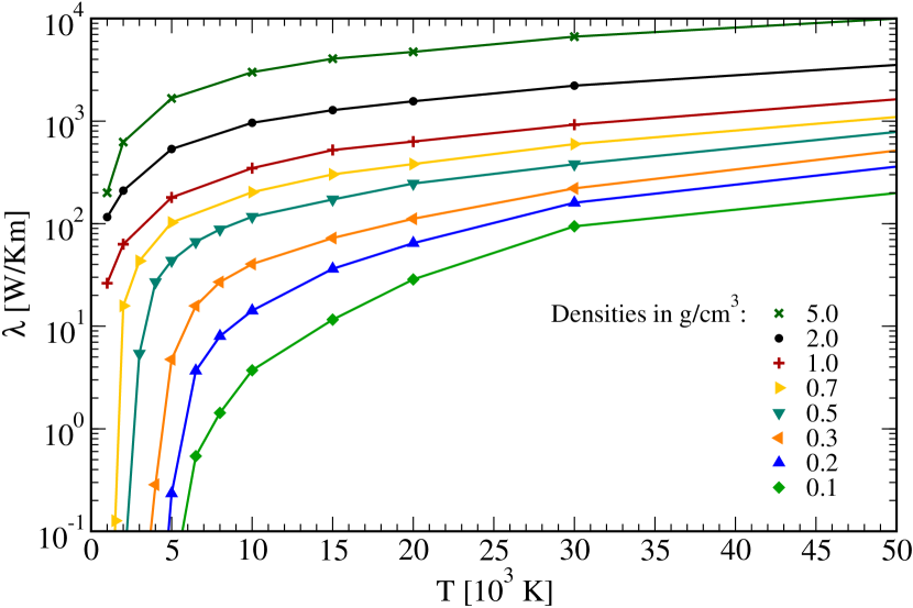
Figure 5: (Color online) Thermal conductivity versus temperature for different densities.

IV.3 Thermopower

The thermopower $\alpha$ characterizes the generation of an electric field as response to a temperature gradient. For most systems this electric field has a direction opposite to the temperature gradient which results in a negative thermopower. The thermopower is most sensitive to changes in the electronic structure since it can be expressed as the derivative of the logarithm of the electronic conductivity with respect to the energy at the Fermi surface. Mott and Davis (1979) Such a relation which is also known as Mott formula follows from the Kubo-Greenwood equation (III) in the degenerate domain under strong scattering conditions.

Interestingly, large positive values for the thermopower were measured in fluid mercury Götzlaff et al. (1988); Hensel and Warren (1999) near the liquid-vapor critical point which is located at $T_{c}=1751$ K and $\varrho_{c}=5.8$ g/cm³. In this region, isotherms of the electrical conductivity near $T_{c}$ show a strong increase with the density which is steepest just at the critical density $\varrho_{c}$. This behavior was assumed to be related to fluctuations in the electron density which are pronounced near the critical point due to critical fluctuations. In particular, a zero of the thermopower was observed exactly at the critical density. The interesting question arises whether or not a zero of the thermopower is a precursor of a first-order phase transition in dense liquids which undergo a nonmetal-to-metal transition. Wide regions with a positive thermopower have been predicted for dense hydrogen by a simple chemical model Höhne et al. (1984) but were not confirmed in an advanced chemical approach Reinholz et al. (1995) by ab initio simulations or by experiments yet.

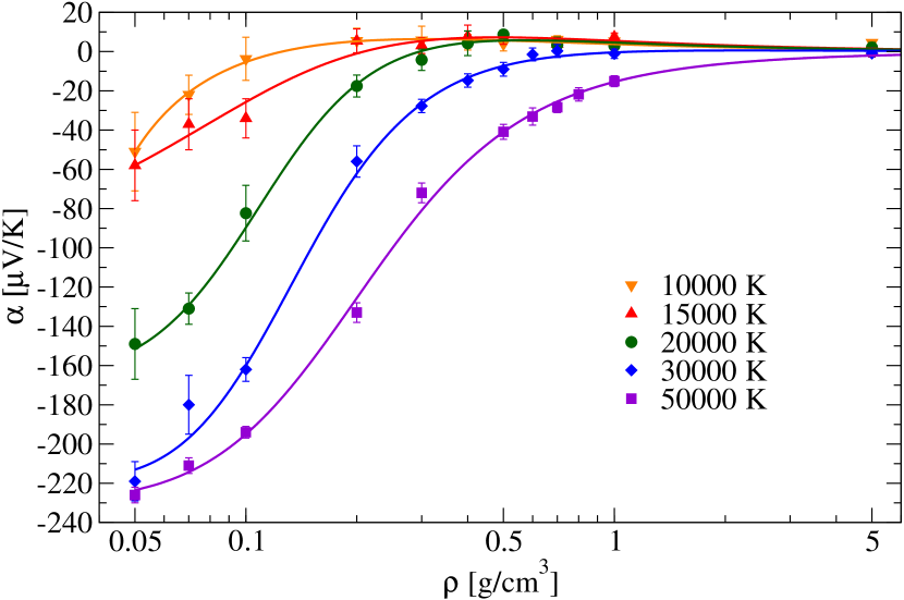
Figure 6: (Color online) Thermopower versus density for different temperatures.

In Fig. 6 isotherms of the thermopower $\alpha$ are plotted as function of the density. The symbols represent the results from the simulations and the error bars show the statistical uncertainties. As guide to the eye, polynomial functions were fitted to the numerical results. The thermopower is mostly negative and reaches a value of about zero at high densities. At lower densities the thermopower decreases. The low density limit of $\alpha=-60.60$ $\mu$V/K is known from the Spitzer theory, see e.g. Ref. Reinholz et al., 1995. With higher temperatures the negative values become systematically larger. We expect that these values become smaller again at low densities to reach the Spitzer limit. The thermopower shows positive mean values below 20000 K and between 0.2 g/cm³ and 0.5 g/cm³. These values are very small and, in fact, about the size of the uncertainties of the respective mean values. We therefore cannot conclude definitely that significantly positive values occur within the accuracy of our ab initio calculations. To answer the question whether or not the zero of the thermopower occurs at the critical point of the liquid-liquid phase transition in dense hydrogen which is predicted Morales et al. (2010); Lorenzen et al. (2010) at about $0.8$ g/cm³, the thermopower has to be evaluated for temperatures below 2000 K since $T_{c}=(1400-2000)$ K. For this region, reasonable results can be given for the electrical and thermal conductivity but not for the thermopower. This is because the values of the Onsager coefficients each decrease over orders of magnitude in systems with a majority of localized electrons while especially the decrease of $L_{12}$ is two orders of magnitude weaker than that of $L_{11}$. This behavior on the one hand causes the second contribution to the thermal conductivity in Eq. (3) to vanish, because $L_{12}$ is squared in the numerator. As a result the thermal conductivity becomes proportional to $L_{22}$ which can be evaluated successfully in this case, as well as $L_{11}$. On the other hand this leads to an enormous increase in the statistical fluctuations of the thermopower, which causes uncertainties that reach hundreds of $\mu$V/K.

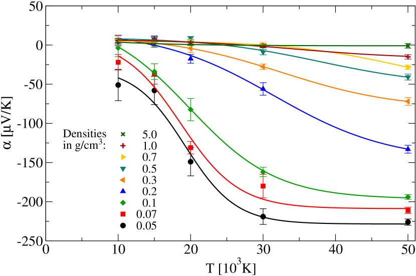
Figure 7: (Color online) Thermopower versus temperature for different densities.

In Fig. 7 isochores of the thermopower $\alpha$ are plotted. The thermopower decreases with higher temperature, which is more pronounced the lower the density is. Positive values appear at low temperatures, but the statistical error is too large to prove this result unambiguously .

IV.4 Lorenz number

The Lorenz number Eq. (4) describes mainly the relation between thermal and electrical conductivity. For simple metals this relation is described via a constant and is known as the Wiedemann-Franz law. For high degeneracy this constant is $L_{0}=\pi^{2}/3$. Ashcroft and Mermin (1976) This relation can be used to easily obtain the thermal conductivity for metals if the electrical conductivity is known. Here we calculate the Lorenz number for dense hydrogen in order to identify the region where the Wiedemann-Franz law is valid. High degeneracy occurs only at sufficiently high densities so that we expect deviations from the Wiedemann-Franz law at lower densities and higher temperatures.

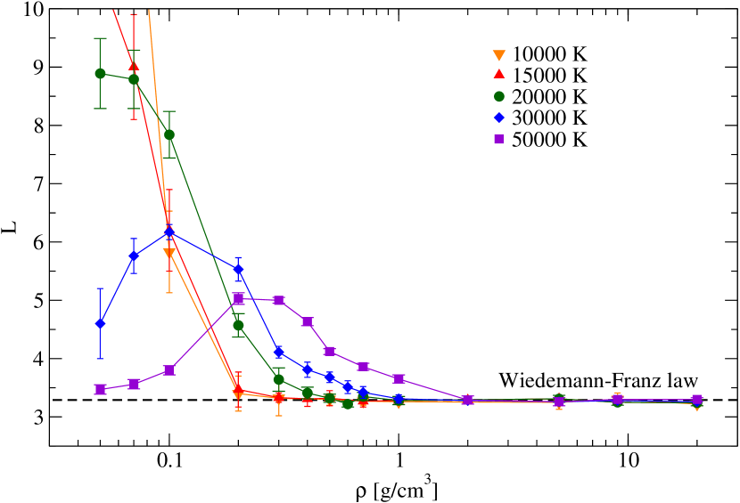
Figure 8: (Color online) Lorenz number versus density for different temperatures. The dashed black line displays the limiting value of $L_{0}=\pi^{2}/3$.

The Lorenz number is shown in Fig. 8 for several temperatures. At densities above 1 g/cm³ the Lorenz number is almost constant and shows no temperature dependence which indicates that the Wiedemann-Franz law is valid there. The value of $L_{0}=\pi^{2}/3$, which is shown by a dashed black line, could be reproduced for each temperature at densities higher than (1-2) g/cm³ within the statistical uncertainties. This behavior is consistent with the metallic-like properties observed already for the conductivity at high densities.

At densities below (1-2) g/cm³ the Lorenz number shows strong deviations from the Wiedemann-Franz law with a pronounced temperature dependence. In particular, the Lorenz number rises strongly with decreasing density. This behavior becomes more pronounced at lower temperatures. On the other hand, at the lower temperatures the validity of the Wiedemann-Franz law extends to smaller densities, e.g. down to 0.2 g/cm³ at 10000 K and 15000 K.

Along the isotherms of 30000 K and 50000 K a maximum can be identified. Thus, at lower densities the Lorenz number decreases again. At 30000 K this maximum is found at a smaller density than at 50000 K and shows a larger value. This indicates that with decreasing temperature the maximum shifts systematically to smaller densities and increases. For temperatures below 30000 K the maximum is not displayed. It appears to be situated at densities below 0.05 g/cm³, which is the minimal density calculated here and which displays the current limit of our computational capabilities. However, we expect a maximum to appear for all temperatures because the Lorenz number is also known exactly at low densities from the Spitzer theory for fully ionized plasmas. Spitzer and Härm (1953) The latter predicts a constant low-density value of 1.5966, see e.g. Ref. Reinholz et al., 1995.

Our results indicate that the deviations from the Wiedemann-Franz law might reach a full order of magnitude in certain regions of density and temperature. Further research will be necessary to investigate this important aspect in more detail. We also expect that certain deviations from the Wiedemann-Franz law occur in warm dense matter of arbitrary composition. In hydrogen, we predict that the Wiedemann-Franz is valid at densities above 2 g/cm³ for temperatures below 50000 K, see Fig. 8.

V Conclusions

We derived formulas for the Onsager transport coefficients $L_{mn}$ within the Kubo theory for application in ab initio simulations. Using these expressions we calculated the electrical and thermal conductivity as well as the thermopower of liquid hydrogen for a wide range of temperatures and densities in the megabar range. In particular, we characterize the nonmetal-to-metal transition in hydrogen by observing a rapid increase in both the electrical and the thermal conductivity. The thermopower shows a trend towards positive values in a region where the critical point of the liquid-liquid phase transition is expected, similar to the behavior of liquid mercury. At low temperatures more accurate calculations will be necessary for this transport coefficient which are beyond the scope of the currently available computer capacity. The ab initio calculation of the Lorenz number shows in addition that the validity of the original Wiedemann-Franz law is limited to the metallic-like regime of hydrogen. The theoretical framework given here can be applied to bulk material calculations for arbitrary materials within FT-DFT-MD.