Nonparametric inference on Lévy measures and copulas

Abstract

In this paper nonparametric methods to assess the multivariate Lévy measure are introduced. Starting from high-frequency observations of a Lévy process $\mathbf{X}$, we construct estimators for its tail integrals and the Pareto–Lévy copula and prove weak convergence of these estimators in certain function spaces. Given $n$ observations of increments over intervals of length $\Delta_{n}$, the rate of convergence is $k_{n}^{-1/2}$ for $k_{n}=n\Delta_{n}$ which is natural concerning inference on the Lévy measure. Besides extensions to nonequidistant sampling schemes analytic properties of the Pareto–Lévy copula which, to the best of our knowledge, have not been mentioned before in the literature are provided as well. We conclude with a short simulation study on the performance of our estimators and apply them to real data.

and T1Supported by the collaborative research center “Statistical modeling of nonlinear dynamic processes” (SFB 823) of the German Research Foundation (DFG).

1 Introduction

The modeling and estimation of dependencies is attracting an increasing attention over the last decades in various fields of science like mathematical finance, actuarial science or hydrology, among others.

In discrete time models, one of the most popular approaches is the concept of copulas which allows one to separate the effects of dependence of a random vector from its univariate marginal behavior. In the bivariate case, the copula of a continuous random vector $(X,Y)$ is the unique function $C\dvtx[0,1]^{2}\rightarrow[0,1]$ for which the identity

$$\mathbb{P}[X\leq x,Y\leq y]=C\bigl{(}\mathbb{P}[X\leq x],\mathbb{P}[Y\leq y]\bigr{)}$$

holds for all $(x,y)\in\mathbb{R}^{2}$. This formula, known as Sklar’s theorem, is usually interpreted in the way that the copula completely characterizes the stochastic dependence between $X$ and $Y$ and hence represents the primary object of interest for investigating dependencies. For introductions to the concept of copulas in the aforementioned fields of science see McNeil, Frey and Embrechts (2005), Frees and Valdez (1998), Genest and Favre (2007) and references therein. The books of Joe (1997) and Nelsen (2006) provide compendiums on the mathematical background and on various parametric models. The huge amount of applications gave rise to a great demand for statistical methods, of which semi- and nonparametric estimation in discrete time i.i.d. models has been investigated in Genest, Ghoudi and Rivest (1995), Fermanian, Radulović and Wegkamp (2004) and Segers (2012), among others.

On the other hand, a huge number of models in applied stochastics relies on an underlying process which is defined in continuous time. A basic tool in this framework is the class of (multidimensional) Lévy processes which provides a flexible way to model empirically observed behavior and includes prime examples such as Brownian motion and the (compound) Poisson process. Statistical methods in this context (including the somewhat more involved one of Itô semimartingales) depend on the nature of the observation schemes which are usually classified as high-frequency and low-frequency setups. In both areas the literature on nonparametrics has grown considerably over the last decade. General overviews on high-frequency statistics can be found in Jacod and Protter (2012) and Mykland and Zhang (2012). To mention only a few approaches in detail which are close to our focus on jump processes we refer to Jacod (2007), Figueroa-López (2009), Aït-Sahalia and Jacod (2009), Bollerslev and Todorov (2011) and Todorov and Tauchen (2011). Seminal papers in the low frequency setting are, for instance, due to Neumann and Reiß (2009) and recently to Nickl and Reiß (2012).

Our aim in this work is to combine both strands of the literature and to provide nonparametric methods to estimate the dependence structure of a multivariate Lévy process. For the sake of brevity we will concentrate on the bivariate case solely, but extensions to the general $d$-dimensional setting are straightforward to obtain as well. Thus, let $\mathbf{X}=(X^{(1)},X^{(2)})$ be a two-dimensional Lévy process with Lévy–Itô decomposition

$$\quad\mathbf{X}_{t}=\mathbf{a}t+\mathbf{B}_{t}+\int_{0}^{t}\int_{\|\mathbf{u}\|\leq 1}\mathbf{u}(\mu-\bar{\mu})(ds,d\mathbf{u})+\int_{0}^{t}\int_{\|\mathbf{u}\|>1}\mathbf{u}\mu(ds,d\mathbf{u}),$$ (1)

where $\mathbf{a}\in\mathbb{R}^{2}$ is a drift vector, $\mathbf{B}$ is a bivariate Brownian motion with some covariance matrix $\Sigma$ and $\mu$ and $\bar{\mu}$ are the jump measure of the Lévy process and its compensator, respectively. It is well-known that the compensator takes the form $\bar{\mu}(ds,d\mathbf{u})=ds\,\nu(d\mathbf{u})$, where $\nu$ is the so-called Lévy measure of $\mathbf{X}$. Given the choice of the truncation function $h(\mathbf{u})=1_{\{\|\mathbf{u}\|>1\}}$, the law of $\mathbf{X}$ is uniquely determined by the Lévy triplet $(\mathbf{a},\Sigma,\nu)$.

As noted above, in the framework of statistics for stochastic processes it is inevitable to lose some words on the underlying observation scheme. We decide to work in a high-frequency setting which means in the simplest case that at stage $n$ one is able to observe one realization of the process $\mathbf{X}$ at the equidistant times $i\Delta_{n}$, $i=0,\ldots,n$, for a mesh $\Delta_{n}\to 0$. A more general setup including irregularly spaced data and asynchronous observations will be provided as well. Within the class of high-frequency settings a further distinction regards the nature of the covered time horizon. Usually, we have either $n\Delta_{n}=T$, corresponding to a finite time horizon (a trading day, say), whereas $n\Delta_{n}\to\infty$ means that the process is eventually observed on the entire time span $[0,\infty)$.

Due to the independence of the continuous part and the jump part of a Lévy process, the analysis of the stochastic nature of $\mathbf{X}$ canonically splits into inference on the covariance matrix $\Sigma$ and inference on the jump measure $\nu$. However, estimation of the characteristics of the Brownian part of $\mathbf{X}$ with or without additional jumps is well understood in the high-frequency setup [among others, see Jacod (2008) for a thorough theory on the behavior of more general Itô semimartingales], so our focus in this paper will be on the jump dependence of the two components. In analogy to standard copulas for random vectors we will employ a concept of a Lévy copula to capture the dependence structure within $\nu$ which dates back to Cont and Tankov (2004) and Kallsen and Tankov (2006). We will follow a slightly different approach due to Klüppelberg and Resnick (2008) and Eder and Klüppelberg (2012), however, and focus on nonparametric methods to assess the closely related Pareto–Lévy copula. Consult also Bollerslev, Todorov and Li (2013) for related work on jump dependence using extreme value theory.

Besides parametric approaches to infer the (Pareto) Lévy copula such as Esmaeili and Klüppelberg (2011), nonparametric methods in this area are hardly available. To the best of our knowledge, the only concept is due to the unpublished work of Laeven (2011) who constructs an estimator for the Lévy copula based on a limit representation involving ordinary copulas. Some asymptotic properties are provided, but no explicit proof is available. On the other hand, since the (Pareto) Lévy copula captures the tendency of the process to have joint (largely negative) jumps, the need for reliable nonparametric estimators is evident from practice, particularly with a view on finance. See, for instance, Böcker and Klüppelberg (2009) who model operational risk via Pareto–Lévy copulas. This convinces us that there is a clear gap in the literature which we aim to fill in this work.

In contrast to Laeven’s method, our approach will be based directly on the defining relation of the Pareto–Lévy copula $\Gamma$ which involves tail integrals of both the Lévy measure and its marginals. For simplicity, we will focus on the spectrally positive case only, that is, we assume that $\mathbf{X}$ has only positive jumps in both directions. Equivalently, the Lévy measure $\nu$ has support on $[0,\infty)^{2}\setminus\{(0,0)\}$, and $\Gamma$ will then naturally be a function on the same space. In the case where all marginal tail integrals have full range $[0,\infty]$, we obtain a representation of $\Gamma$ as a functional of those, and we propose to estimate $\Gamma$ by using appropriate estimators for the tail integrals. It turns out that in order to do so, we are forced to work in the high-frequency setting with infinite time horizon, that is, $n\Delta_{n}\to\infty$. Under some rather mild assumptions we are then able to prove weak convergence of a suitably standardized version of $\hat{\Gamma}-\Gamma$ in a certain function space, which will be our main result. As a by-product, we obtain a Donsker theorem for the bivariate Lévy measure as well; a result which is similar in spirit to the recent work of Nickl and Reiß (2012), but in a high-frequency setting rather than a low-frequency world.

The paper is organized as follows: Section 2 is devoted to a brief discussion on jump dependence of bivariate Lévy processes. We summarize the concept of Pareto–Lévy copulas and derive some of their analytical properties. In Section 3 we define estimators for bivariate tail integrals, as well as for their associated Pareto–Lévy copulas. Weak convergence of these estimators is discussed in Section 4, while Section 5 is devoted to deviations from the ideal sampling scheme. A brief discussion of our results, a small simulation study and a real data example are provided in Section 6, whereas some conclusions are given in Section 7. Finally, the main steps of the proofs are postponed to Section Appendix, while more technical details are treated in a supplementary Appendix.

2 Jump dependence and the Pareto–Lévy copula

Suppose that we are given a bivariate Lévy process $\mathbf{X}$ of the form (1) where $\nu$ denotes its Lévy measure. As already stated in the Introduction, one assumption will be that $\nu$ has support on $[0,\infty)^{2}\setminus\{(0,0)\}$, which means that both components of $\mathbf{X}$ only have positive jumps. This condition is for notational convenience in first place, as we will see later that one can follow a similar approach in order to estimate the jump dependence in the other three quadrants as well.

Let us review some recent concepts of jump dependence. The basic quantity in this framework is the bivariate tail integral $U$ associated with $\nu$, which, for the moment, will be defined as a function from $[0,\infty]^{2}\setminus\{(0,0)\}$ to $\mathbb{R}$ by

$$U(\mathbf{x})=\nu\bigl{(}[x_{1},\infty]\times[x_{2},\infty]\bigr{)},\qquad\mathbf{x}=(x_{1},x_{2}).$$

From the theory of Lévy processes it is well known that this quantity gives the average amount of jumps of $\mathbf{X}$ which fall into the interval $[x_{1},\infty]\times[x_{2},\infty]$ during a time period of length one. Since $\mathbf{X}$ has càdlàg paths, $U(\mathbf{x})$ is necessarily finite. In the same way, we are able to introduce marginal tail integrals. Precisely, let $U_{i}\dvtx[0,\infty]\to[0,\infty]$, $i=1,2$, be defined via

$$U_{1}(x_{1})=\nu\bigl{(}[x_{1},\infty]\times\mathbb{R}\bigr{)}\quad\mbox{and}\quad U_{2}(x_{2})=\nu\bigl{(}\mathbb{R}\times[x_{2},\infty]\bigr{)}.$$

Again, $U_{i}(x_{i})$ is finite for $x_{i}>0$, but in the infinite activity case we may have $U_{i}(0)=\infty$, $i=1,2$.

It is obvious that the entire information about $\nu$ is contained in the tail integral $U$. Therefore, just as for regular copulas, one might be interested in splitting $U$ into several functions which are related to the jump behavior of $\mathbf{X}$ in the marginals (naturally given by the univariate tail integrals $U_{i}$) and a Lévy copula $C$ which captures the specific tendency of $\mathbf{X}$ to have joint jumps. Having this intuition in mind, Cont and Tankov (2004) provided the following definition.

Definition 2.1.

A bivariate Lévy copula for Lévy processes with positive jumps is a function $C\dvtx[0,\infty]^{2}\setminus\{(\infty,\infty)\}\to[0,\infty)$ which: [(iii)]

is grounded, that is, $C(x,0)=C(0,x)=0$ for all $x\in[0,\infty]$;

has uniform margins, so $C(x,\infty)=C(\infty,x)=x$ for all $x\in[0,\infty)$;

is 2-increasing, that is, $C(x_{1},x_{2})-C(x_{1},y_{2})-C(y_{1},x_{2})+C(y_{1},y_{2})\geq 0$ for all $x_{1}\leq y_{1}$ and $x_{2}\leq y_{2}$.

The main result on Lévy copulas is a version of Sklar’s famous theorem which states that for each tail integral $U$ with marginals $U_{1}$ and $U_{2}$ there exists a Lévy copula $C$ such that

$$U(\mathbf{x})=C\bigl{(}U_{1}(x_{1}),U_{2}(x_{2})\bigr{)},\qquad\mathbf{x}=(x_{1},x_{2})\in[0,\infty]^{2}\setminus\bigl{\{}(0,0)\bigr{\}},$$

holds. Similarly to the usual copula, $C$ is uniquely defined on $\operatorname{ran}U_{1}\times\operatorname{ran}U_{2}$ and, in particular, $C$ is globally unique if $\operatorname{ran}U_{i}=[0,\infty]$ for $i=1,2$. This becomes our second main assumption. In that case, we obtain a representation of $C$ via

$$C(\mathbf{u})=U\bigl{(}U_{1}^{-}(u_{1}),U_{2}^{-}(u_{2})\bigr{)},\qquad\mathbf{u}=(u_{1},u_{2})\in[0,\infty]^{2}\setminus\bigl{\{}(\infty,\infty)\bigr{\}},$$

where, for any $f\dvtx(0,\infty]\to[0,\infty)$ which is nonincreasing, left-continuous and satisfies $f(\infty)=0$, $f^{-}\dvtx(0,\infty]\to[0,\infty)$ denotes the generalized inverse function

$$f^{-}(z)=\inf\bigl{\{}x>0\dvtx f(x)\leq z\bigr{\}}$$ (2)

and where we use the convention $f^{-}(0)=\infty$.

The inverse statement of Sklar’s theorem is true as well: knowledge of the marginals $U_{i}$ and the Lévy copula $C$ completely determines $U$ and thus in turn $\nu$. A drawback of the approach of Cont and Tankov (2004) is, however, that $C$ is not a tail integral itself. This is in contrast to the regular copula of a random vector which couples marginal distribution functions and is a bivariate distribution function on its own. This circumstance makes the interpretation of a Lévy copula quite difficult, and for that reason it appears to be natural to focus on an alternative notion of copula in this setting.

Definition 2.2.

A bivariate Pareto–Lévy copula for Lévy processes with positive jumps is a function $\Gamma\dvtx[0,\infty]^{2}\setminus\{(0,0)\}\to[0,\infty)$ which: [(iii)]

is grounded, that is, $\Gamma(u,\infty)=\Gamma(\infty,u)=0$ for all $u\in(0,\infty]$;

has Pareto margins, so $\Gamma(u,0)=\Gamma(0,u)=1/u$ for all $u\in(0,\infty]$;

is 2-increasing.

As usual, we set $1/\infty=0$ and vice versa. Following Eder and Klüppelberg (2012), Sklar’s theorem now reads as follows: given $U$ and its marginals, we have

$$U(\mathbf{x})=\Gamma\bigl{(}1/{U_{1}(x_{1})},1/{U_{2}(x_{2})}\bigr{)},\qquad\mathbf{x}=(x_{1},x_{2})\in[0,\infty]^{2}\setminus\bigl{\{}(0,0)\bigr{\}}$$

for some unique Pareto–Lévy copula $\Gamma$, and we obtain the relation

$$\qquad\Gamma(\mathbf{u})=U\bigl{(}U_{1}^{-}(1/u_{1}),U_{2}^{-}(1/u_{2})\bigr{)},\qquad\mathbf{u}=(u_{1},u_{2})\in[0,\infty]^{2}\setminus\bigl{\{}(0,0)\bigr{\}}.$$ (3)

The difference to the approach of Cont and Tankov (2004) is that the marginals of $\Gamma$ correspond to Pareto tails, which are the tail integrals of a 1-stable Lévy process on the positive half line. Since $\Gamma$ is 2-increasing as well, it is a simple task to deduce that it satisfies the properties of a tail integral of a spectrally positive Lévy process as claimed. Thus the Pareto–Lévy copula allows for the interpretation that the marginals of $\nu$ are standardized to the Lévy measures of a 1-stable Lévy process, which is similar in spirit to the ordinary copula concept where marginals are standardized to uniform distributions.

Finally, we collect some basic properties of Pareto–Lévy copulas, some of which already have been stated in Cont and Tankov (2004) and Kallsen and Tankov (2006) in the context of Lévy copulas.

Proposition 2.3

Every Pareto Lévy copula $\Gamma$ has the following properties: [(iii)]

(Lipschitz continuity). $|\Gamma(\mathbf{u})-\Gamma(\mathbf{v})|\leq|\frac{1}{u_{1}}-\frac{1}{v_{1}}|+|\frac{1}{u_{2}}-\frac{1}{v_{2}}|$.

(Monotonicity). $\Gamma$ is 2-increasing and the functions $\Gamma(u,\cdot)$ and $\Gamma(\cdot,u)$ are nonincreasing for each fixed $u\geq 0$.

(Fréchet-Hoeffding bounds). $\Gamma_{\perp}\leq\Gamma\leq\Gamma_{\|}$, where $\Gamma_{\|}(\mathbf{u})=(u_{1}\vee u_{2})^{-1}$ and $\Gamma_{\perp}(\mathbf{u})=u_{1}^{-1}1_{\{u_{2}=0\}}+u_{2}^{-1}1_{\{u_{1}=0\}}$ denote the Pareto Lévy copulas corresponding to perfect positive dependence and to independence, respectively.

(Partial derivatives). $\dot{\Gamma}_{1}(u_{1},0)=-u_{1}^{-2}$ and $\dot{\Gamma}_{1}(u_{1},\infty)=0$. For fixed $u_{2}\in(0,\infty)$, the partial derivative $\dot{\Gamma}_{1}(u_{1},u_{2})$ exists for almost all $u_{1}\in(0,\infty)$, and for such $u_{1}$ and $u_{2}$ we have

$$0\geq\dot{\Gamma}_{1}(u_{1},u_{2})\geq-u_{1}^{-2}.$$

Furthermore, the mapping $u_{2}\mapsto\dot{\Gamma}_{1}(u_{1},u_{2})$ is defined and nondecreasing almost everywhere. Analogous results hold for the partial derivative with respect to $u_{2}$.

3 Estimation of bivariate tail integrals and Pareto–Lévy copulas

In the following we are interested in the construction of an estimator $\hat{\Gamma}_{n}$ for $\Gamma$ which is based on relation (3) and empirical versions of the tail integrals $U$, $U_{1}$ and $U_{2}$. Such estimators have, for instance, been discussed in Figueroa-López (2008) in the univariate setting, and we will transfer them naturally to the bivariate case.

Before we introduce these empirical versions, it turns out to be convenient to slightly change the domain of $U$. Since by assumption no negative jumps are involved, we have $\nu([x_{1},\infty]\times[0,\infty])=\nu([x_{1},\infty]\times[-\infty,\infty])$ for each $x_{1}>0$, and similarly for the second component. Therefore it is equally well possible to define $U$ in the same way as before, but as a function $U\dvtx\mathbb{H}\to\mathbb{R}$, where

$$\mathbb{H}=(0,\infty]^{2}\cup\bigl{(}\{-\infty\}\times(0,\infty]\bigr{)}\cup\bigl{(}(0,\infty]\times\{-\infty\}\bigr{)}.$$

Note that, on the stripes through $-\infty$, $U$ corresponds to the marginal tail integrals $U_{1}$ and $U_{2}$, respectively.

Our estimator for the function $U$ will be defined on $\mathbb{H}$ as well. We set

$$U_{n}(\mathbf{x})=\frac{1}{k_{n}}\sum_{j=1}^{n}1_{\{\Delta_{j}^{n}X^{(1)}\geq x_{1},\Delta_{j}^{n}X^{(2)}\geq x_{2}\}},\qquad\mathbf{x}=(x_{1},x_{2}),$$ (4)

where $k_{n}=n\Delta_{n}$ and $\Delta_{j}^{n}X^{(i)}=X^{(i)}_{j\Delta_{n}}-X^{(i)}_{(j-1)\Delta_{n}}$ denotes the $j$th increment of $X^{(i)}$, $i=1,2$. Having the role of the stripes through $-\infty$ in mind, we obtain empirical versions of the univariate tail integrals through

$$U_{n,1}(x_{1})=U_{n}(x_{1},-\infty)=\frac{1}{k_{n}}\sum_{j=1}^{n}1_{\{\Delta_{j}^{n}X^{(1)}\geq x_{1}\}},\qquad x_{1}\in(0,\infty],$$ (5)

and analogously for $U_{n,2}$. Weak convergence of $U_{n}$ in an appropriate function space is established in Theorem 4.2 below.

The underlying idea behind $U_{n}$ is rather natural, given the interpretation of $U$ as the average number of jumps of a certain size during the unit interval. Stationarity and indepedence of increments of a Lévy process ensure that the same behavior is to be expected over intervals of arbitrary size, as long as $U$ is standardized accordingly. Therefore, a canonical idea is to count joint large increments of $X^{(1)}$ and $X^{(2)}$, as they indicate joint large jumps over the corresponding time interval. This is precisely what $U_{n}$ does.

Remark 3.1.

Several comments regarding the conditions on the underlying sampling scheme are in order. [(iii)]

In order for $U_{n}$ to be consistent, it is necessary to be in the high-frequency setting with infinite time horizon, that is, $k_{n}\to\infty$. If we restrict ourselves to observations from a fixed time interval $[0,T]$, there are only finitely many jumps larger than a given size, which is clearly not sufficient to draw inference on the entire distribution of the jumps.

In reality, one usually neither sees both components of $\mathbf{X}$ at the same time nor has a regular sampling scheme of observations with distance $\Delta_{n}$. Therefore, the methods proposed in this section need to be sharpened when dealing with a more general setup including irregularly spaced data and asynchronous observations which is done in Section 5 below. The same comment applies concerning microstructure noise issues, in which case the distribution of the increments depends heavily on the distribution of the noise variables added.

The method of counting large increments in order to identify jumps is a feature of observation schemes at high frequency. In a low frequency world, with $\Delta_{n}=\Delta$ being fixed, one rather observes a superposition of jumps and increments of the continuous part and needs deconvolution techniques to distinguish between both effects.

In order to construct an empirical version of (3) recall the definition of a generalized inverse function in (2).

Definition 3.2.

Let $U$ be the tail integral of a bivariate Lévy process with positive jumps and $U_{1}$, $U_{2}$ be its marginal tail integrals. Using their empirical versions (4) and (5) we define, for any $\mathbf{u}=(u_{1},u_{2})\in[0,\infty]^{2}\setminus\{(0,0)\}$, the empirical Pareto–Lévy copula as

$$\hat{\Gamma}_{n}(\mathbf{u})=U_{n}\bigl{(}\overline{U_{n,1}^{-}(1/u_{1})},\overline{U_{n,2}^{-}(1/u_{2})}\bigr{)},$$ (6)

where $U_{n,i}^{-}$ is the generalized inverse function of $U_{n,i}$ as defined in (2), with the convention that $U_{n,i}^{-}(1/\infty)=U_{n,i}^{-}(0)=\infty$ and where $\overline{a}=a1_{\{a>0\}}-\infty 1_{\{a=0\}}$ for some $a\in[0,\infty]$. Finally, we set $U_{n}(-\infty,-\infty)=n/k_{n}$.

Remark 3.3.

In order to understand why $\overline{a}$ is introduced, suppose that we are interested in estimating $\Gamma(u_{1},0)$ even though it is known to take the value $1/u_{1}$. Our estimator becomes $U_{n}({U_{n,1}^{-}(1/u_{1})},-\infty)$ then, which is in general close to $1/u_{1}$ due to the definition of $U_{n,1}$. On the other hand, if we forget about $\overline{a}$, we obtain $U_{n}({U_{n,1}^{-}(1/u_{1})},0)$ which only counts those increments of $\mathbf{X}$ where the first component exceeds ${U_{n,1}^{-}(1/u_{1})}$ and the second one is nonnegative. Due to the existence of a Brownian part in $\mathbf{X}$, however, we cannot expect these two estimators to be close, since a nonnegligible number of increments in the second component is indeed negative, and thus this estimator is considerably smaller than $\hat{\Gamma}(u_{1},0)$.

Remark 3.4.

In the general case of arbitrary jumps, a similar construction allows for the estimation of $\Gamma$ in the interior of each of the four quadrants separately. Indeed, Eder and Klüppelberg (2012) give a general notion of tail integrals and Pareto–Lévy copulas in their Definition 4, and from Sklar’s theorem in this context (which is their Theorem 1) we know that the same relation as (3) holds for $\mathbf{u}\in(\mathbb{R}\setminus\{0\})^{2}$ and determines $\Gamma$ uniquely. For the sake of brevity we dispense with the entire theory in this setting.

4 Results on weak convergence

Our aim in this section is to prove results on weak convergence of both estimators, and we begin with such a claim for $U_{n}$, as this theorem is used later to show weak convergence of $\hat{\Gamma}_{n}$. Before we come to the main theorems, let us briefly resume our assumptions on $\nu$ which mostly have already been given in the previous paragraphs.

Assumption 4.1.

Let $\mathbf{X}$ be a bivariate Lévy process with the representation (1). The following assumptions on $\nu$ are in order: [(iii)]

$\nu$ has support $[0,\infty)^{2}\setminus\{(0,0)\}$.

On this set it takes the form $\nu(d\mathbf{u})=s(\mathbf{u})\,d\mathbf{u}$ for a positive Lévy density $s$ which satisfies

$$\sup_{u\in M_{\eta}}\bigl{(}\bigl{|}s(\mathbf{u})\bigr{|}+\bigl{\|}\nabla s(\mathbf{u})\bigr{\|}\bigr{)}<\infty$$

for any $\eta\in(0,\infty)^{2}$, where

$$M_{\eta}=(\eta,\infty)^{2}\cup\bigl{(}\{0\}\times(\eta,\infty)\bigr{)}\cup\bigl{(}(\eta,\infty)\times\{0\}\bigr{)},$$

and $\nabla s$ denotes the gradient of $s$ on $(\eta,\infty)^{2}$ and the univariate derivative on the stripes through 0, respectively.

$\nu$ has infinite activity, that is, $\nu([0,\infty)\times[0,\infty))=\infty$.

Assumption 4.1(ii) had not been stated previously. It is used to prove a second order condition regarding the difference between $U$ and the expectation of $U_{n}$, for which we generalize a result due to Figueroa-López and Houdré (2009) from the univariate setting to the multidimensional case. Continuity and (strict) monotonicity of the marginal tail integrals as claimed before are obvious consequences of it.

We begin with a result on weak convergence of $U_{n}$, and to this end we have to define the function space on which the asymptotics take place. Let $\mathcal{B}_{\infty}(\mathbb{H})$ be the space of all functions $f\dvtx\mathbb{H}\to\mathbb{R}$ which are bounded on any subset of $\mathbb{H}$ that is bounded away from the origin and from the points $(-\infty,0)$ and $(0,-\infty)$. We consider the metric inducing the topology of uniform convergence on those subsets, defined by

$$d(f,g)=\sum_{k=1}^{\infty}2^{-k}\bigl{(}\|f-g\|_{T_{k}}\wedge 1\bigr{)},$$

where $T_{k}=[1/k,\infty]^{2}\cup(\{-\infty\}\times[1/k,\infty])\cup([1/k,\infty]\times\{-\infty\})$ and $\|f\|_{T_{k}}=\sup_{\mathbf{u}\in T_{k}}|f(\mathbf{u})|$. This space is a complete metric space, and a sequence converges in $\mathcal{B}_{\infty}(\mathbb{H})$, if and only if it converges uniformly on each $T_{k}$.

Theorem 4.2.

Assume that $\mathbf{X}$ is a Lévy process satisfying (i) and (ii) of Assumption 4.1. If the observation scheme meets the conditions

$$\Delta_{n}\to 0,\qquad k_{n}\to\infty,\qquad\sqrt{k_{n}}\Delta_{n}\to 0,$$ (7)

then we have

$$\gamma_{n}(\mathbf{x})=\sqrt{k_{n}}\bigl{\{}U_{n}(\mathbf{x})-U(\mathbf{x})\bigr{\}}\stackrel{{\scriptstyle w}}{{\longrightarrow}}{\mathbb{B}}(\mathbf{x})$$

in $(\mathcal{B}_{\infty}(\mathbb{H}),d)$, where ${\mathbb{B}}$ is a tight, centered Gaussian process with covariance

$$\mathbb{E}\bigl{[}{\mathbb{B}}(\mathbf{x}){\mathbb{B}}(\mathbf{y})\bigr{]}=U(\mathbf{x}\vee\mathbf{y})=U(x_{1}\vee y_{1},x_{1}\vee y_{2}).$$

The sample paths of ${\mathbb{B}}$ are uniformly continuous on each $T_{k}$ with respect to the pseudo distance

$$\rho(\mathbf{x},\mathbf{y})=\mathbb{E}\bigl{[}\bigl{(}{\mathbb{B}}(\mathbf{x})-{\mathbb{B}}(\mathbf{y})\bigr{)}^{2}\bigr{]}^{1/2}=\bigl{|}U(\mathbf{x})-U(\mathbf{y})\bigr{|}^{1/2}.$$

For the proof of Theorem 4.2 the following lemma is extremely useful. Its univariate version is a special case of a more general result in Figueroa-López and Houdré (2009).

Lemma 4.3.

Suppose that (i) and (ii) of Assumption 4.1 hold and let $\delta>0$ be fixed. Then there exist constants $K=K(\delta)$ and $t_{0}=t_{0}(\delta)$ such that the uniform bound

$$\bigl{|}\mathbb{P}\bigl{(}X_{t}^{(1)}\geq x_{1},X_{t}^{(2)}\geq x_{2}\bigr{)}-t\nu\bigl{(}[x_{1},\infty)\times[x_{2},\infty)\bigr{)}\bigr{|}<Kt^{2}$$

holds for all $\mathbf{x}=(x_{1},x_{2})\in[\delta,\infty]^{2}\cup(\{-\infty\}\times[\delta,\infty])\cup([\delta,\infty]\times\{-\infty\})$ and $0<t<t_{0}$.

Remark 4.4.

Lemma 4.3 is used in the proof of Theorem 4.2 to show that the bias of $U_{n}$ is of order $\Delta_{n}$. It is this result which is responsible for the condition $\sqrt{k_{n}}\Delta_{n}\to 0$ in (7) as the latter secures that this bias term is negligible in the asymptotics. If one has $\sqrt{k_{n}}\Delta_{n}\to c>0$, instead, together with a stronger condition on differentiability of $s(\mathbf{u})$, a bias term will appear in Theorem 4.2. Precisely, generalizing a result from Figueroa-López and Houdré (2009) again, we obtain

$$\mathbb{P}\bigl{(}X_{t}^{(1)}\geq x_{1},X_{t}^{(2)}\geq x_{2}\bigr{)}=t\nu\bigl{(}[x_{1},\infty)\times[x_{2},\infty)\bigr{)}+t^{2}d_{2}(\mathbf{x})/2+O\bigl{(}t^{3}\bigr{)},$$

uniformly in the same sense as above, with

$$d_{2}(\mathbf{x}) = 2\biggl{(}\int_{x_{2}}^{\infty}s(x_{1},w_{2})\,dw_{2}a_{\varepsilon}^{1}+\int_{x_{1}}^{\infty}s(w_{1},x_{2})\,dw_{1}a_{\varepsilon}^{2}\biggr{)}$$

$${}-\biggl{(}\int_{x_{2}}^{\infty}s_{1}(x_{1},w_{2})\,dw_{2}\Sigma_{11}+\int_{x_{1}}^{\infty}s_{2}(w_{1},x_{2})\,dw_{1}\Sigma_{22}-2s(x_{1},x_{2})\Sigma_{12}\biggr{)}$$

$${}-2\int\int_{0}^{1}(1-\beta)\biggl{(}\int_{x_{2}-\beta u_{2}}^{\infty}s_{1}(x_{1}-\beta u_{1},w_{2})\,dw_{2}u_{1}^{2}$$

$$\hskip 86.0pt{}+\int_{x_{1}-\beta u_{1}}^{\infty}s_{2}(w_{1},x_{2}-\beta u_{2})\,dw_{1}u_{2}^{2}$$

$$\hskip 101.0pt{}-2s(x_{1}-\beta u_{1},x_{2}-\beta u_{2})u_{1}u_{2}\biggr{)}\,d\beta\nu_{\varepsilon}(d\mathbf{u})$$

$${}+\int\int s(\mathbf{z})\bar{c}_{\varepsilon}(\mathbf{z})s(\mathbf{w})\bar{c}_{\varepsilon}(\mathbf{w})1_{\{\mathbf{w}+\mathbf{z}\geq x\}}\,d\mathbf{z}\,d\mathbf{w}-2\lambda_{\varepsilon}\nu\bigl{(}[\mathbf{x},\infty)\bigr{)}.$$

Here, $\varepsilon>0$ denotes an auxiliary variable used to simplify the expression, and for all unexplained notation we refer to the proof of Lemma 4.3. Under the condition $\sqrt{k_{n}}\Delta_{n}\to c>0$ above, it can be shown that the asymptotic bias in Theorem 4.2 takes the form $cd_{2}(\mathbf{x})/2$. Note that it is possible to derive a representation for $d_{2}(\mathbf{x})$ independently of $\varepsilon$, which takes an even more complicated form. This expression is given explicitly in the supplementary material, alongside with a sketch of a proof.

Before we come to the result on $\hat{\Gamma}_{n}$, let us introduce an oracle estimator for $\Gamma$. We set, for any $\mathbf{u}=(u_{1},u_{2})\in[0,\infty]^{2}\setminus\{(0,0)\}$,

$$\widetilde{\Gamma}_{n}(\mathbf{u})=U_{n}\bigl{(}U_{1}^{-}(1/u_{1}),U_{2}^{-}(1/u_{2})\bigr{)},$$

which means that we replace the inverses of the empirical marginal tail integrals by the unobservable true ones. Thanks to Theorem 4.2 we obtain weak convergence of a restricted version of this intermediate estimator in the space $\mathcal{B}_{\infty}((0,\infty]^{2})$ of all real functions on $(0,\infty]^{2}$ that are bounded on sets which are bounded away from the origin. In a similar sprit as before, we equip this space with the metric $d(f,g)=\sum_{k=1}^{\infty}2^{-k}(\|f-g\|_{T_{k}}\wedge 1)$, where $T_{k}=[1/k,\infty]^{2}$. Setting $\mathbf{x}=(U_{1}^{-}(1/u_{1}),U_{2}^{-}(1/u_{2}))$ and observing that $U_{i}^{-}(k)\geq k^{\prime}>0$, the continuous mapping theorem immediately yields the following result.

Corollary 4.5.

Under the conditions of Theorem 4.2 we have

$$\widetilde{\alpha}_{n}(\mathbf{u})=\sqrt{k_{n}}\bigl{(}\widetilde{\Gamma}_{n}(\mathbf{u})-\Gamma(\mathbf{u})\bigr{)}\stackrel{{\scriptstyle w}}{{\longrightarrow}}\mathbb{B}\bigl{(}U_{1}^{-}(1/u_{1}),U_{2}^{-}(1/u_{2})\bigr{)}$$

in $(\mathcal{B}_{\infty}((0,\infty]^{2}),d)$, with $\mathbb{B}$ as defined in Theorem 4.2.

From a statistical point of view, there is no loss in information when estimating $\Gamma(\mathbf{u})$ on $(0,\infty]^{2}$ instead of the entire domain $[0,\infty]^{2}\setminus\{(0,0)\}$, since a Pareto–Lévy copula is grounded by definition and thus known on stripes through 0. This remark remains valid for the final result of this section as well, which is on weak convergence of the estimator $\hat{\Gamma}_{n}(\mathbf{u})$.

Theorem 4.6.

Assume that $\mathbf{X}$ is a Lévy process satisfying Assumption 4.1. If (7) holds, then we have

$$\alpha_{n}(\mathbf{u})=\sqrt{k_{n}}\bigl{(}\hat{\Gamma}_{n}(\mathbf{u})-\Gamma(\mathbf{u})\bigr{)}\stackrel{{\scriptstyle w}}{{\longrightarrow}}\mathbb{G}(\mathbf{u})$$

in $(\mathcal{B}_{\infty}((0,\infty]^{2}),d)$. Here, the process $\mathbb{G}$ is defined as

$$\mathbb{G}(\mathbf{u})=\widetilde{\mathbb{G}}(\mathbf{u})+u_{1}^{2}\dot{\Gamma}_{1}(\mathbf{u})\widetilde{\mathbb{G}}(u_{1},-\infty)+u_{2}^{2}\dot{\Gamma}_{2}(\mathbf{u})\widetilde{\mathbb{G}}(-\infty,u_{2}),$$ (8)

where $\widetilde{\mathbb{G}}$ denotes a tight centered Gaussian field on $\mathbb{H}$ with covariance structure

$$\mathbb{E}\bigl{[}\widetilde{\mathbb{G}}(\mathbf{u})\widetilde{\mathbb{G}}(\mathbf{v})\bigr{]}=\Gamma(\mathbf{u}\vee\mathbf{v})=\Gamma(u_{1}\vee v_{1},u_{2}\vee v_{2})$$

using the convention $\Gamma(u,-\infty)=\Gamma(-\infty,u)=1/u$. The sample paths of $\widetilde{\mathbb{G}}$ are uniformly continuous on each $T_{k}$ with respect to the pseudo distance

$$\rho(\mathbf{u},\mathbf{v})=\mathbb{E}\bigl{[}\bigl{(}\widetilde{\mathbb{G}}(\mathbf{u})-\widetilde{\mathbb{G}}(\mathbf{v})\bigr{)}^{2}\bigr{]}^{1/2}=\bigl{|}\Gamma(\mathbf{u})-\Gamma(\mathbf{v})\bigr{|}^{1/2}.$$

If both coordinates of $\mathbf{u}$ are distinct from $\infty$, then $\dot{\Gamma}_{i}(\mathbf{u})$ exists as a consequence of (3) and Assumption 4.1, and $\mathbb{G}(\mathbf{u})$ is well-defined. On the other hand, if one of the components equals $\infty$, we have $\widetilde{\mathbb{G}}(\mathbf{u})=0$ almost surely; and also $\dot{\Gamma}_{1}(u_{1},\infty)=0$ and $\dot{\Gamma}_{2}(\infty,u_{2})=0$ from Proposition 2.3. Hence, the right-hand side of (8) is well defined as well, and we have $\mathbb{G}(\mathbf{u})=0$ almost surely in this case.

5 Deviations from the regular setting

Up to now, the results in this paper have been shown in the ideal setting of observing a Lévy process at equidistant and synchronous times. With a view to applications, it is obvious that these assumptions are not realistic in practice. For example, due to the stylized facts of financial time series, pure Lévy processes possessing independent increments are too restrictive for the modeling of financial time series. Also, multiple stock prices are usually traded at different time points, contradicting our assumed observation scheme. Ways to overcome the latter problem have so far only been discussed in the context of volatility estimation [a remarkable exception is Comte and Genon-Catalot (2010)], and it is known that limit theorems usually differ from the ones for regular observation times and are obtained under quite restrictive assumptions only, particularly when the time points are asynchronous. See, for example, Aït-Sahalia and Mykland (2003, 2004), Hayashi and Yoshida (2005, 2008), Mykland and Zhang (2009) or Hayashi, Jacod and Yoshida (2011).

Our aim in this section is to develop a concise theory which allows for a consistent estimation of the Lévy measure also in case of irregular observations or when one observes a model with time-varying drift and diffusion part. We will focus in particular on inference on the distribution function $U(\mathbf{x})$, since weak convergence of the empirical Pareto–Lévy copula process carries over using the same results on Hadamard differentiability as in the proof of Theorem 4.6. Furthermore, we will indicate how results change in case of microstructure noise and why standard methods for diffusions do not carry over to our setting.

5.1 Nonequidistant sampling schemes

The first generalization regards the assumption of an equidistant sampling scheme which we no longer assume to hold. Instead, suppose from now on that the observation times are given by deterministic $t_{j}^{n}$, $j=1,\ldots,m_{n}$, where we set $k_{n}=t_{m_{n}}^{n}$ as before. The results carry over to the case of random sampling as well, at least if the observations times are independent of $\mathbf{X}$.

Still, the most natural estimator appears to be given by counting joint large increments, which results in setting

$$V_{n}(\mathbf{x})=\frac{1}{k_{n}}\sum_{j=1}^{m_{n}}1_{\{\Delta_{j}^{n}X^{(1)}\geq x_{1},\Delta_{j}^{n}X^{(2)}\geq x_{2}\}},$$ (9)

where we have defined $\Delta_{j}^{n}X^{(i)}=X^{(i)}_{t_{j}^{n}}-X^{(i)}_{t_{j-1}^{n}}$ (with $t_{0}^{n}=0$) in the same spirit as before. Finally, let $\pi_{n}=\max_{j=1,\ldots,m_{n}}(t_{j}^{n}-t_{j-1}^{n})$.

Theorem 5.1.

Assume that $\mathbf{X}$ is a Lévy process satisfying (i) and (ii) of Assumption 4.1. If furthermore the observation scheme meets the conditions

$$k_{n}\to\infty,\qquad\pi_{n}\to 0,\qquad\frac{1}{\sqrt{k_{n}}}\sum_{j=1}^{m_{n}}\bigl{(}t_{j}^{n}-t_{j-1}^{n}\bigr{)}^{2}\to 0,$$ (10)

then we have $\sqrt{k_{n}}\{V_{n}(\mathbf{x})-U(\mathbf{x})\}\stackrel{{\scriptstyle w}}{{\longrightarrow}}{\mathbb{B}}(\mathbf{x})$ in $(\mathcal{B}_{\infty}(\mathbb{H}),d)$, where ${\mathbb{B}}$ is the same Gaussian process as in Theorem 4.2.

Remark 5.2.

Even though the assumption $\pi_{n}\to 0$ ensures that we remain in a genuine high-frequency setting, it is not necessary in general and only used here to simplify the proofs. Suppose, for example, that we have $t_{1}^{n}=1$ for all $n$, whence it is obviously not possible to infer the Lévy measure consistently over the interval $[0,1]$. This, however, does not affect the validity of Theorem 5.1 per se, since a single increment of $\mathbf{X}$ contributes with either $1/k_{n}$ or zero to $V_{n}$, so its influence is negligible in the asymptotics, and as $k_{n}\to\infty$ holds, one can equally well use the observations over $[1,k_{n}]$ to estimate the function $U$.

5.2 Asynchronous sampling schemes

Suppose now that both components of $\mathbf{X}$ are observed at different time stamps. We call $r_{j}^{n}$, $j=1,\ldots,m^{1}_{n}$, the series of observations times connected with the process $X^{(1)}$, whereas $s_{\ell}^{n}$, $\ell=1,\ldots,m^{2}_{n}$, belongs to the second component $X^{(2)}$. For simplicity only, we assume that the endpoints coincide, that is $r_{m_{n}^{1}}=s_{m_{n}^{2}}=k_{n}$. As before, we denote with $\pi_{n}^{i}$ the mesh of the $i$th time series.

In this situation it is less obvious how to count the number of joint large jumps, as increments over $X^{(1)}$ and $X^{(2)}$ are in general never computed over the same time intervals. In spirit of Hayashi and Yoshida (2005), however, it appears reasonable to construct a naïve estimator from counting those pairs of large increments which are computed over at least overlapping intervals. Of course, in this case it may happen that jumps at different times (but close nearby) are treated as joint ones. For this reason it is important to assume additional properties of the jump measures which make such an event unlikely.

Assumption 5.3.

Let $\nu^{i}(dx)$ be the univariate Lévy measures for $i=1,2$. We assume that $\nu^{i}(dx)=\nu_{1}^{i}(dx)+\nu_{2}^{i}(dx)$ for mutually singular measures $\nu_{1}^{i}$ and $\nu_{2}^{i}$, given by

$$\nu_{1}^{i}(dx)=a_{i}\frac{1+|x|^{\gamma_{i}}f_{i}(x)}{|x|^{1+\beta_{i}}}1_{\{0<x\leq 1\}}\,dx$$

with $0\leq f_{i}(x)\leq K$, $\gamma_{i}\geq 0$, $a_{i}\geq 0$ and $\nu_{2}^{i}$ such that $\nu_{2}^{i}(dx)=s^{i}(x)\,dx$ for some Lévy density $s^{i}$ such that $\int(|x|^{\beta^{\prime}_{i}}\wedge 1)s^{i}(x)\,dx<\infty$, where $0\leq\beta^{\prime}_{i}<\beta_{i}<2$.

This condition means basically that the behavior of small jumps in both components is similar to the one of $\beta_{i}$-stable processes. Such assumptions are often used in high-frequency statistics for jump processes; cf., for example, Aït-Sahalia and Jacod (2009) and related work. Our estimator for $U(\mathbf{x})$ now reads as follows:

$$W_{n}(\mathbf{x})=\frac{1}{k_{n}}\sum_{j=1}^{m_{n}^{1}}\sum_{\ell=1}^{m_{n}^{2}}1_{\{\Delta_{j}^{n}X^{(1)}\geq x_{1},\Delta_{\ell}^{n}X^{(2)}\geq x_{2}\}}1_{\{(r_{j-1}^{n},r_{j}^{n}]\cap(s_{\ell-1}^{n},s_{\ell}^{n}]\neq\varnothing\}}.$$ (11)

Under slightly more restrictive conditions on the sampling scheme than before, we obtain the following result on weak convergence.

Theorem 5.4.

Let $\mathbf{X}$ be a Lévy process satisfying Assumptions 4.1(i) and (ii) and Assumption 5.3. Setting $\beta=\max(\beta_{1},\beta_{2})$ assume further that the sampling scheme satisfies $\max(\pi_{n}^{1},\pi_{n}^{2})\to 0$ as well as

$$\frac{1}{\sqrt{k_{n}}}\sum_{j=1}^{m_{n}^{1}}\bigl{(}r_{j}^{n}-r_{j-1}^{n}\bigr{)}^{{(\beta+2)}/{(\beta+1)}}\to 0\qquad\mbox{if }\beta>1$$

and

$$\frac{1}{\sqrt{k_{n}}}\sum_{j=1}^{m_{n}^{1}}\bigl{(}r_{j}^{n}-r_{j-1}^{n}\bigr{)}^{3/2-\delta}\to 0\qquad\mbox{if }\beta\leq 1$$

for some $\delta\in(0,1/2)$, and similarly for the increments involving $s_{\ell}^{n}$. Then we have $\sqrt{k_{n}}\{W_{n}(\mathbf{x})-U(\mathbf{x})\}\stackrel{{\scriptstyle w}}{{\longrightarrow}}{\mathbb{B}}(\mathbf{x})$ in $(\mathcal{B}_{\infty}(\mathbb{H}),d)$, where ${\mathbb{B}}$ is the same Gaussian process as in Theorem 4.2.

Remark 5.5.

It is remarkable that even though methods similar to the case of volatility estimation work for inference on $U$ as well, the results look quite different in this setting: in case of irregular observations, only very few additional assumptions on the observation scheme are necessary, which is in contrast to the restrictive conditions of Hayashi and Yoshida (2008) regarding covolatility. This happens, however, at the cost of additional assumptions on the structure of the underlying Lévy process. When dealing with irregular sampling times, we obtain the same central limit theorem as for equidistant ones. This has again no direct connection to volatility estimation, as the corresponding result in Mykland and Zhang (2009) comes with a different variance.

Remark 5.6.

There is a variety of models which satisfy Assumptions 4.1 and 5.3. Among the simplest are stable processes in both components, coupled by some Lévy copula which is twice continuously differentiable away from the origin (e.g., the Clayton one).

5.3 Observing semimartingales

In this section we discuss briefly deviations from assumption (1) on the observed process. Suppose that the underlying process is an Itô semimartingale with the representation

$$\mathbf{X}_{t} = \int_{0}^{t}\mathbf{a}_{s}\,ds+\int_{0}^{t}\sigma_{s}\,d\mathbf{B}_{s}$$

$${}+\int_{0}^{t}\int_{\|\mathbf{u}\|\leq 1}\mathbf{u}(\mu-\bar{\mu})(ds,d\mathbf{u})+\int_{0}^{t}\int_{\|\mathbf{u}\|>1}\mathbf{u}\mu(ds,d\mathbf{u})$$

instead, where $\mathbf{a}\in\mathbb{R}^{2}$ and $\sigma\in\mathbb{R}^{2\times 2}$ are bounded and left-continuous processes. Recall that all central limit theorems proposed before deal with sums of large increments of $\mathbf{X}$, interpreted as coming from large jumps over the same time intervals. This intuition is based on the fact that the probability of the continuous Lévy part to become large over small time intervals is exponentially small, and therefore it is likely that these claims remain valid under weaker conditions on $\mathbf{X}$ as well. The following theorem states that this is indeed the case, if we assume that all sampling schemes satisfy similar growth conditions as in Theorem 5.4.

Theorem 5.7.

Let $\mathbf{X}$ be an Itô semimartingale as above, and assume that the respective assumptions on the sampling schemes from Theorems 4.6, 5.1 and 5.4 are satisfied. Assume further that the sampling schemes satisfy

$$\sqrt{k_{n}}\Delta_{n}^{1/2-\delta}\to 0\quad\mbox{or}\quad\frac{1}{\sqrt{k_{n}}}\sum_{j=1}^{m_{n}}\bigl{(}t_{j}^{n}-t_{j-1}^{n}\bigr{)}^{3/2-\delta}\to 0$$

for Theorems 4.6 or 5.1, respectively, and for some $\delta\in(0,1/2)$. Then, the weak convergence results of the respective theorems hold.

The proof relies on replacing increments of $\mathbf{X}$ by corresponding increments of a pure jump Lévy process in order to apply theorems on weak convergence based on sums of independent observations. At this stage, the additional conditions on the sampling scheme come into play. Weaker conditions might be sufficient here, if one was able to prove weak convergence based on some type of conditional independence instead, then using different approximations for increments of $\mathbf{X}$.

5.4 Microstructure noise

An important issue regarding high-frequency data is the presence of microstructure noise, in which case one does not observe the plain Lévy process, but

$$Z^{(j)}_{i\Delta_{n}}=X^{(j)}_{i\Delta_{n}}+V^{(j)}_{i\Delta_{n}},$$

where the $V^{(j)}_{i\Delta_{n}}$, $i=1,\ldots,n$, $j=1,2$, are i.i.d. processes, independent of $X$, which satisfy $\mathbb{E}[V^{(j)}_{i\Delta_{n}}]=0$ and have moments of all order. In this case, our estimator for the Lévy measure does not work anymore. To see this, let us for simplicity stick to the univariate setting. We have

$$U_{n}(x)=\frac{1}{k_{n}}\sum_{i=1}^{n}1_{\{\Delta_{i}^{n}Z\geq x\}}$$

now, and if there is a positive probability of $P(\Delta_{i}^{n}V\geq x)$, then $U_{n}(x)$ will behave like $\Delta_{n}^{-1}P(\Delta_{i}^{n}V\geq x)$ which diverges to infinity. On the other hand, if $P(\Delta_{i}^{n}V\geq x)=0$, then $U_{n}(x)$ is still bounded, but will rather estimate a convolution of jumps and noise than the plain jump measure.

Microstructure noise issues are well understood in the context of diffusions. However, it appears that none of the standard methods for diffusion processes [let us mention the multiscale approach by Zhang, Mykland and Aït-Sahalia (2005) and the kernel-based one due to Barndorff-Nielsen et al. (2008)] can directly be applied in our context. Even the pre-averaging approach by Jacod et al. (2009), which provides a general concept for diminishing the influence of the noise by retaining information about increments of $X$, fails when one is interested in the Lévy measure. In the following, we will briefly discuss these issues.

For an auxiliary sequence $l_{n}$ and some piecewise differentiable function $g$ on $[0,1]$ with $g(0)=g(1)=0$, Jacod et al. (2009) discuss $\widetilde{Z}_{i}^{n}=\widetilde{X}_{i}^{n}+\widetilde{V}_{i}^{n}$, where, for an arbitrary $Y$ and $i=0,\ldots,n-l_{n}$,

$$\widetilde{Y}_{i}^{n}=\sum_{j=1}^{l_{n}}g(j/l_{n})\Delta_{i+j}^{n}Y.$$

While $\widetilde{X}_{i}^{n}$ can be seen as some kind of generalized increment which still bears similar information as the plain $\Delta_{i}^{n}X$, we have

$$\widetilde{V}_{i}^{n}=-g(1/l_{n})V_{i\Delta_{n}}+\sum_{j=1}^{l_{n}-1}\bigl{(}g(j/l_{n})-g\bigl{(}(j+1)/l_{n}\bigr{)}\bigr{)}V_{(i+j)\Delta_{n}}=O_{p}\bigl{(}l_{n}^{-1/2}\bigr{)}.$$

Here we use both piecewise differentiability of $g$ and the assumptions concerning $g$ on the boundary of $[0,1]$. Therefore the larger $l_{n}$ becomes, the less important is the contamination by noise.

For this reason, estimation based on pre-averaging usually works in the way that one proceeds as usual, but replaces the standard estimators by ones based on $\widetilde{Z}_{i}^{n}$. If $l_{n}$ is rather large compared with $n$, it is reasonable to replace $\widetilde{Z}_{i}^{n}$ with $\widetilde{X}_{i}^{n}$ in the asymptotics and thus to recover full information of $X$. In our setting this would lead to an estimator of the form

$$\widetilde{U}_{n}(x)=\frac{1}{k_{n}}\sum_{i=0}^{\lfloor n/l_{n}\rfloor-1}1_{\{\widetilde{Z}_{il_{n}}^{n}\geq x\}},$$

where the $\widetilde{Z}_{il_{n}}^{n}$ are computed over nonoverlapping intervals to retain i.i.d. terms in the sum. As noted above, for large $l_{n}$ it is equally well possible to discuss $\widetilde{U}_{n}^{X}(x)$ which is defined similarly to $\widetilde{U}_{n}(x)$ above, but using $\widetilde{X}_{il_{n}}^{n}$ instead of $\widetilde{Z}_{il_{n}}^{n}$. This procedure, however, does not result in an estimator for the Lévy distribution function $U(y)$. The reason is that the leading term in an expansion of $P(\widetilde{X}_{0}^{n}\geq y)$ is due to a single large jump within $[0,l_{n}\Delta_{n}]$. In this case, its contribution to $\widetilde{X}_{0}^{n}$ depends on its exact position within the interval, as it has to be standardized by $g(j/l_{n})$ accordingly. For example, if the jump occurs in the small interval $[(j-1)\Delta_{n},j\Delta_{n}]$, it is not important whether the jump is larger than $y$, but whether it is larger than $y/g(j/l_{n})$. Since the jump time is uniformly distributed, one can show formally that

$$P\bigl{(}\widetilde{X}_{il_{n}}^{n}\geq y\bigr{)} = \Delta_{n}\sum_{j=1}^{l_{n}}U\bigl{(}y/g(j/l_{n})\bigr{)}+O\bigl{(}l_{n}^{2}\Delta_{n}^{2}\bigr{)}$$

$$= l_{n}\Delta_{n}\int_{0}^{1}U\bigl{(}y/g(x)\bigr{)}\,dx+o(l_{n}\Delta_{n}),$$

which proves that $\widetilde{U}_{n}^{X}(y)$ converges to $\int_{0}^{1}U(y/g(x))\,dx$ and is therefore not consistent for $U(y)$. Construction of a consistent estimator for the Lévy measure in case of microstructure noise thus seems to be a challenging topic for future research.

6 Discussion, simulations and an illustration

6.1 An asymptotic comparison

Suppose a statistician has knowledge of the marginal tail integrals. In this case, the results in Section 4 provide two competitive asymptotically unbiased estimators for the Pareto–Lévy copula, namely the oracle estimator $\widetilde{\Gamma}_{n}$ exploiting knowledge of the marginals and the empirical Pareto–Lévy copula $\hat{\Gamma}_{n}$ ignoring this additional information. The following proposition gives a partial answer to the question of which estimator is (asymptotically) preferable. Perhaps surprisingly, ignoring the additional knowledge decreases the asymptotic variance under certain growth conditions on $\Gamma$. A similar observation has recently been made in the context of copula estimation; see Genest and Segers (2010).

Proposition 6.1

Suppose that the Pareto–Lévy copula $\Gamma$ has continuous first-order partial derivatives and that the functions

$$u_{1}\mapsto u_{1}\Gamma(u_{1},u_{2})=\frac{\Gamma(u_{1},u_{2})}{\Gamma(u_{1},0)},\qquad u_{2}\mapsto u_{2}\Gamma(u_{1},u_{2})=\frac{\Gamma(u_{1},u_{2})}{\Gamma(0,u_{2})}$$ (12)

are nondecreasing for fixed $u_{2}\in(0,\infty]$ and $u_{1}\in(0,\infty]$, respectively. Then the Gaussian fields $\mathbb{G}$ and $\widetilde{\mathbb{G}}$ satisfy the inequality

$$\operatorname{Cov}\bigl{\{}\mathbb{G}(\mathbf{u}),\mathbb{G}(\mathbf{v})\bigr{\}}\leq\operatorname{Cov}\bigl{\{}\widetilde{\mathbb{G}}(\mathbf{u}),\widetilde{\mathbb{G}}(\mathbf{v})\bigr{\}}$$

for all $\mathbf{u},\mathbf{v}\in(0,\infty]^{2}$. Particularly, $\operatorname{Var}\{\mathbb{G}(\mathbf{u})\}\leq\operatorname{Var}\{\widetilde{\mathbb{G}}(\mathbf{u})\}$.

Under the assumptions of Proposition 6.1 the condition in (12) is equivalent to

$$u_{1}\dot{\Gamma}_{1}(\mathbf{u})+\Gamma(\mathbf{u})\geq 0,\qquad u_{2}\dot{\Gamma}_{2}(\mathbf{u})+\Gamma(\mathbf{u})\geq 0$$

for each $\mathbf{u}=(u_{1},u_{2})\in(0,\infty]^{2}$, which is easily accessible for most parametric classes of Pareto–Lévy copulas. For instance, for the Clayton Pareto–Lévy copula given by

$$\Gamma(\mathbf{u})=\bigl{(}u_{1}^{\theta}+u_{2}^{\theta}\bigr{)}^{-1/\theta}$$

we have

$$u_{1}\dot{\Gamma}_{1}(\mathbf{u})+\Gamma(\mathbf{u})=\bigl{(}u_{1}^{\theta}+u_{2}^{\theta}\bigr{)}^{-1/\theta-1}u_{2}^{\theta},\qquad u_{2}\dot{\Gamma}_{2}(\mathbf{u})+\Gamma(\mathbf{u})=\bigl{(}u_{1}^{\theta}+u_{2}^{\theta}\bigr{)}^{-1/\theta-1}u_{1}^{\theta},$$

which is readily seen to be nonnegative. In Figure 1 we depict the graph of the asymptotic relative efficiency

$$[0,2]^{2}\to[0,\infty),\qquad\mathbf{u}\mapsto{\operatorname{Var}\bigl{\{}\mathbb{G}(\mathbf{u})\bigr{\}}}/{\operatorname{Var}\bigl{\{}\widetilde{\mathbb{G}}(\mathbf{u})\bigr{\}}}$$

of the oracle estimator $\widetilde{\Gamma}_{n}$ to the empirical Pareto–Lévy copula $\hat{\Gamma}_{n}$ for $\mathbf{u}\in[0,2]^{2}$. The Clayton parameter is chosen as $\theta=0.5$. Close to the axis the relative efficiency decreases to $0$, while the maximal relative efficiency is attained on the diagonal with a value of $21/32\approx 0.656$. Even in this best case, the difference is seen to be substantial.

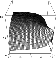
Figure 1: The graph of the asymptotic relative efficiency of $\widetilde{\Gamma}_{n}$ to $\hat{\Gamma}_{n}$ for the Clayton Pareto–Lévy copula with $\theta=0.5$.

6.2 Simulation study

In order to obtain an impression on the performance of the asymptotic results stated in the previous section we will discuss some finite sample properties concerning Theorems 4.2 and 4.6. In both cases, the setting is as follows: we simulate (essentially) two $1/2$ stable subordinators, that is, both tail integrals are given by $U_{i}(x)=(\pi x)^{-1/2}$, which are coupled by a Clayton–Pareto–Lévy copula with $\theta=1/2$. Sometimes, we add two independent Brownian motions with variance $1/2$ each, and sometimes, we assume to observe the pure jump processes only.

Recall that the rate of convergence is $k_{n}^{-1/2}$ [which, in light of the results in Figueroa-López and Houdré (2009), appears to be natural in the context of estimating the Lévy measure]. Hence, a larger $k_{n}$ suggests a better approximation by the limiting Gaussian process, whereas Remark 4.4 indicates that the magnitude of the bias grows with $k_{n}$ as well. Both intuitive properties are visible from the simulation study provided in the following and from additional results which we do not show for the sake of brevity.

We begin with a thorough simulation study for a fixed number of observations $n=22\mbox{,}500$, where we run the simulation $500$ times each. We have decided to keep the size of the data set fixed in order to work out the effects that different choices of $k_{n}$, or, equivalently, of $\Delta_{n}$, have on the finite sample performance of our estimators. Otherwise, if one fixes $k_{n}$ or $\Delta_{n}$ and investigates increasing sample sizes, it will in general be hard to tell whether a possible gain in the MSE (say) is due to a more reasonable trade-off between bias and variance or just to more observations. We briefly discuss these issues at the end of this section in an additional simulation study with a fixed number of days $k_{n}$.

Table 1: Empirical bias and (co)variances of $\sqrt{k_{n}}(U_{n}(\mathbf{x})-U(\mathbf{x}))$ for various choices of $k_{n}$. Upper five lines: pure subordinator; lower five lines: subordinator${}+{}$Brownian motion

$\bolds{x,y}$	$\bolds{2,2}$		$\bolds{1,1}$		$\bolds{0.5,0.5}$		2, 0.5	2, 1	1, 0.5
$\bolds{k_{n}}$	$\operatorname{\mathbf{bias}}$	$\operatorname{\mathbf{var}}$	$\operatorname{\mathbf{bias}}$	$\operatorname{\mathbf{var}}$	$\operatorname{\mathbf{bias}}$	$\operatorname{\mathbf{var}}$	$\operatorname{\mathbf{cov}}$	$\operatorname{\mathbf{cov}}$	$\operatorname{\mathbf{cov}}$
50	$-0.0106$	0.1007	$-0.0077$	0.1400	$0.0023$	0.1915	0.0988	0.0978	0.1376
75	$-0.0330$	0.0972	$-0.0229$	0.1453	$-0.0395$	0.1956	0.1015	0.1001	0.1435
100	$0.0168$	0.1021	$0.0223$	0.1375	$0.0341$	0.1893	0.0996	0.0927	0.1300
150	$0.0037$	0.1061	$0.0154$	0.1480	$0.0470$	0.2180	0.1073	0.1106	0.1531
250	$0.0282$	0.0931	$0.0547$	0.1269	$0.0951$	0.1845	0.0900	0.0865	0.1245
50	$-0.0281$	0.0893	$-0.0120$	0.1208	$-0.0042$	0.1863	0.0840	0.0854	0.1233
75	$0.0252$	0.0949	$0.0115$	0.1187	$0.0226$	0.1861	0.0861	0.0894	0.1216
100	$0.0126$	0.0922	$0.0043$	0.1320	$0.0401$	0.1940	0.0933	0.0932	0.1323
150	$-0.0085$	0.0929	$-0.0127$	0.1337	$0.0277$	0.1991	0.0931	0.0962	0.1371
250	$0.0128$	0.1101	$0.0236$	0.1395	$0.0765$	0.1938	0.1049	0.1044	0.1369

Despite the fact that we have proven weak convergence of our estimators in certain function spaces, we restrict ourselves to an analysis of the finite dimensional properties of our estimators. Let us begin with the asympotics in Theorem 4.2 for which we estimate $U(x,x)$ for $x=2,1,0.5$. Note that we have $\operatorname{Cov}(\mathbb{B}(\mathbf{x}),\mathbb{B}(\mathbf{y}))=(32\pi)^{-1/2}\approx 0.0997$ whenever $\mathbf{x}$ or $\mathbf{y}$ equals $(2,2)$, whereas $\operatorname{Cov}(\mathbb{B}(\mathbf{x}),\mathbb{B}(\mathbf{y}))=(16\pi)^{-1/2}\approx 0.1410$ if the “larger” vector is $(1,1)$ and finally $\operatorname{Var}(\mathbb{B}(\mathbf{x}))=(8\pi)^{-1/2}\approx 0.1995$ for $\mathbf{x}=(0.5,0.5)$. Table 1 gives estimated bias and (co)variance for various choices of the number of trading days, $k_{n}$. These values are picked in such a way that they belong to reasonable scenarios in practice. The smallest one, $k_{n}=50$, corresponds to $\Delta_{n}^{-1}=450$ or sampling frequencies of about a minute, for which microstructure noise already become an issue. On the other hand, the largest choice of $k_{n}=250$ necessitates data from a process whose jump behavior is homogeneous for quite a long period of time, namely about one year.

Generally, the theoretical (co)variances are well reproduced in both situations, even though the results look probably a bit better in the first five lines. This is of course no surprise, since additional Brownian increments make it harder to infer on the jump measure. In order to assess how well the normal approximation works apart from bias and variance, Figure 2 gives QQ-plots for the medium choice of $k_{n}=75$. These plots confirm that the finite sample properties are indeed satisfying, despite the discrete nature of the test statistic which simply counts exceedances of certain levels and is rescaled afterward.

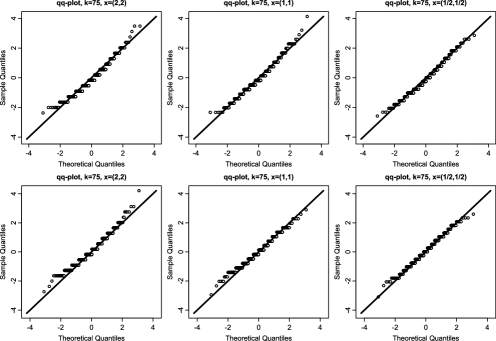
Figure 2: QQ-plots of the empirical quantiles of $\sqrt{k_{n}}(U_{n}(\mathbf{x})-U(\mathbf{x}))$ divided by their sample standard deviation vs. the theoretical quantiles of the standard normal distribution. Upper three pictures: pure subordinator; lower three pictures: subordinator${}+{}$Brownian motion.

Let us come to the estimation of the Pareto–Lévy copula. We proceed in the same way as before and discuss convergence of the finite dimensional distributions only. For simplicity, we estimate $\Gamma(x,x)$ for $x=2,1,0.5$ again, but these are of course different quantities now. In this case, the variances compute to $\operatorname{Var}(\mathbb{G}(\mathbf{x}))=21/(128x)$, which becomes approximately $0.0820$ for $x=2$, $0.1641$ for $x=1$, and $0.3281$ for $x=0.5$. Also, for $x>y$ we have $\operatorname{Cov}(\mathbb{G}(\mathbf{x}),\mathbb{G}(\mathbf{y}))=7/32(1/x-\Gamma(x,y))$. Therefore $\operatorname{Cov}(\mathbb{G}(\mathbf{2}),\mathbb{G}(\mathbf{0.5}))\approx 0.0608$, $\operatorname{Cov}(\mathbb{G}(\mathbf{2}),\mathbb{G}(\mathbf{1}))\approx 0.0718$, and $\operatorname{Cov}(\mathbb{G}(\mathbf{1}),\mathbb{G}(\mathbf{0.5}))\approx 0.1437$. We state their empirical versions in Table 2.

In this case the growth in bias for larger $k_{n}$ is clearly visible, and we also have a larger bias when estimating $\Gamma(0.5,0.5)$. Overall, however, the results are satisfying again, and we see from the QQ-plot in Figure 3 that the normal approximation works very well for $k_{n}=75$, no matter if a Brownian motion is added or not.

Table 2: Empirical bias and (co)variances of $\sqrt{k}(\hat{\Gamma}_{n}(\mathbf{x})-\Gamma(\mathbf{x}))$ for various choices of $k_{n}$. Upper five lines: pure subordinator; lower five lines: subordinator${}+{}$Brownian motion

$\bolds{x,y}$	$\bolds{2,2}$		$\bolds{1,1}$		$\bolds{0.5,0.5}$		2, 0.5	2, 1	1, 0.5
$\bolds{k_{n}}$	$\operatorname{\mathbf{bias}}$	$\operatorname{\mathbf{var}}$	$\operatorname{\mathbf{bias}}$	$\operatorname{\mathbf{var}}$	$\operatorname{\mathbf{bias}}$	$\operatorname{\mathbf{var}}$	$\operatorname{\mathbf{cov}}$	$\operatorname{\mathbf{cov}}$	$\operatorname{\mathbf{cov}}$
50	$0.0141$	0.0827	0.0455	0.1740	0.0863	$0.3520$	0.0777	0.0668	0.1599
75	$-0.0082$	0.0874	0.0173	0.1653	0.1252	$0.3428$	0.0740	0.0690	0.1459
100	$0.0502$	0.0783	0.0894	0.1708	0.1748	$0.3400$	0.0685	0.0508	0.1547
150	$0.0356$	0.0862	0.1182	0.1646	0.3176	$0.3324$	0.0744	0.0698	0.1421
250	$0.0505$	0.0732	0.1493	0.1605	0.5625	$0.313$	0.0678	0.0568	0.1390
50	$0.0345$	0.0790	0.0560	0.1637	0.1021	$0.3263$	0.0699	0.0639	0.1389
75	$0.0091$	0.0886	0.0753	0.1760	0.1522	$0.3508$	0.0832	0.0729	0.1522
100	$0.0312$	0.0745	0.0776	0.1530	0.1480	$0.3033$	0.0610	0.0558	0.1305
150	$0.0284$	0.0866	0.0988	0.1694	0.2074	$0.3337$	0.0746	0.0725	0.1486
250	$0.0602$	0.0762	0.1515	0.1528	0.3012	$0.3452$	0.0675	0.0545	0.1455

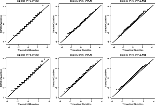
Figure 3: QQ-plots of the empirical quantiles of $\sqrt{k_{n}}(\hat{\Gamma}_{n}(\mathbf{x})-\Gamma(\mathbf{x}))$ divided by their sample standard deviation vs. the theoretical quantiles of the standard normal distribution. Upper three pictures: pure subordinator; lower three pictures: subordinator${}+{}$Brownian motion.

Finally, let us briefly discuss the performance of our estimators in case of a fixed number $k_{n}$ and for increasing sampling frequencies $\Delta_{n}^{-1}$. We restrict ourselves to the case of estimating $U$ for a pure subordinator, as other settings lead to similar results. For $k_{n}$ fixed, one would expect that choosing a rather low frequency yields the worst results since in this case the bias is the largest, or, equivalently, the jumps are most difficult to detect. On the other hand, for growing $\Delta_{n}^{-1}$ this bias becomes smaller, but otherwise not much is to be gained, as the sampling frequency does not affect the rate of convergence. The results in Table 3, where we consider all possible combinations of $k_{n},\Delta_{n}^{-1}\in\{50,100,150,200\}$, support these findings. For financial applications this means that, provided sufficient data is available, a trade-off has to be made: on the one hand, one should choose the frequency as high as possible; but on the other hand, due to microstructure noise issues, care is needed regarding a possibly oversized frequency.

Table 3: Empirical bias and (co)variances of $\sqrt{k_{n}}(U_{n}(\mathbf{x})-U(\mathbf{x}))$ for various choices of $k_{n}$ and $\Delta_{n}^{-1}$. In all cases: pure subordinator

$\bolds{x,y}$	$\bolds{2,2}$		$\bolds{1,1}$		$\bolds{0.5,0.5}$		2, 0.5	2, 1	1, 0.5
$\bolds{\Delta_{n}^{-1}}$	$\operatorname{\mathbf{bias}}$	$\operatorname{\mathbf{var}}$	$\operatorname{\mathbf{bias}}$	$\operatorname{\mathbf{var}}$	$\operatorname{\mathbf{bias}}$	$\operatorname{\mathbf{var}}$	$\operatorname{\mathbf{cov}}$	$\operatorname{\mathbf{cov}}$	$\operatorname{\mathbf{cov}}$
$k_{n}=50$
50	$0.0338$	0.1065	$0.0285$	0.1425	$0.0648$	0.2072	0.1037	0.1017	0.1407
100	$0.0010$	0.0976	$0.0005$	0.1316	$0.0354$	0.1972	0.0942	0.0936	0.1336
150	$0.0007$	0.1058	$0.0138$	0.1445	$0.0204$	0.2038	0.1044	0.1043	0.1446
200	$0.0027$	0.1005	$0.0059$	0.1370	$0.0286$	0.1928	0.0991	0.0935	0.1343
$k_{n}=100$
50	$0.0194$	0.1032	$0.0589$	0.1424	$0.1071$	0.2052	0.1024	0.1026	0.1421
100	$-0.0200$	0.1007	$0.0017$	0.1466	$0.0175$	0.1981	0.1034	0.1025	0.1434
150	$0.0150$	0.1002	$0.0175$	0.1480	$0.0275$	0.1999	0.1021	0.0979	0.1444
200	$0.0202$	0.0957	$0.0103$	0.1326	$0.0299$	0.2059	0.0953	0.1017	0.1392
$k_{n}=150$
50	$0.0312$	0.1034	$0.0659$	0.1450	$0.1286$	0.2080	0.1037	0.1057	0.1437
100	$0.0132$	0.0988	$0.0205$	0.1369	$0.0489$	0.2092	0.0960	0.0984	0.1407
150	$0.0037$	0.1061	$0.0154$	0.1480	$0.0470$	0.2180	0.1073	0.1106	0.1531
200	$-0.0098$	0.0948	$-0.0122$	0.1315	$-0.0156$	0.1891	0.0923	0.0884	0.1299
$k_{n}=200$
50	$0.0134$	0.0990	$0.0468$	0.1334	$0.1237$	0.1947	0.0932	0.0892	0.1306
100	$-0.0012$	0.0995	$0.0136$	0.1415	$0.0554$	0.2092	0.0986	0.1003	0.1437
150	$-0.0006$	0.0966	$0.0217$	0.1371	$0.0413$	0.1966	0.0944	0.0950	0.1372
200	$0.0011$	0.0934	$0.0292$	0.1371	$0.0305$	0.2074	0.0942	0.0961	0.1416

6.3 Illustration

In the present section we are going to apply the estimation techniques developed in the previous sections to infer on the jump dependence of some specific financial data set.

More precisely, we consider the logarithm of one-minute Nasdaq stock prices of Apple Inc. and Microsoft Corporation in the third quarter of 2012, which consists of $62$ trading days. After some cleaning of the corresponding time series we obtain a two-dimensional data sample of increments (log returns) of size $n=21\mbox{,}864$. From the simulation results in Section 6.2 we know that the choice $k_{n}=62$ yields a reasonable trade-off between bias and variance.

Due to missing observations or errors in data, we formally apply the procedure from Section 5.2, though the observations are in principle quite close to a regular sampling scheme. We have chosen a frequency of one minute returns in order to have a large amount of data while not being too much affected by microstructure effects which our method does not correct for; see Section 5.4. Note that the results in this paper are stated for observations of a bivariate semimartingale with a constant Lévy measure which is probably a too simple model for a bivariate price process. What might be less restrictive, is to assume a time-homogeneous Pareto–Lévy copula, if one is only interested in the dependence structure of the assets.

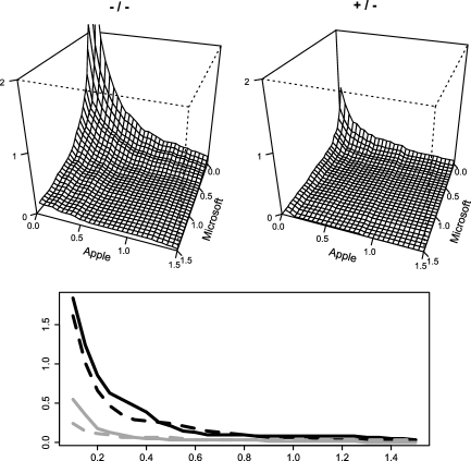
Figure 4: Upper two pictures: empirical Pareto–Lévy copulas for the $(-/-)$ and the $(+/-)$ dependence. Lower picture: empirical Pareto–Lévy copulas along the diagonal for $(-/-)$ (black solid line), $(+/+)$ (black dashed), $(+/-)$ (gray solid) and $(-/+)$ (gray dashed) dependence.

For this reason, we are interested in margin-free estimates of the jump dependence only, which means that we restrict ourselves to the estimation of the Pareto–Lévy copula $\Gamma$. There are four possible types of jump dependence: positive jumps in both components ($+/+$), positive jumps in the log-returns of Apple may be associated with negative jumps in the log-returns of Microsoft ($+/-$), and vice versa ($-/+$), and negative jumps in both components ($-/-$). To obtain estimates in the latter three cases, we simply use negative log-returns in the corresponding components in the definition of $\hat{\Gamma}_{n}$.

The results are depicted in Figure 4. In the two upper pictures, we plot the graph of the empirical Pareto–Lévy copula on the set $[0.05,1.5]^{2}$ for the dependencies $(-/-)$ and $(+/-)$, respectively. The corresponding graphs for $(+/+)$ and $(-/+)$, respectively, look very similar and are therefore omitted. In the lower picture, we plot the restriction of the graphs of the empirical Pareto–Lévy copula to the main diagonal for all four kinds of dependence.

The following are the main findings:

• The dependence between positive or negative jumps in both components ($+/+$ and $-/-$) is generally much stronger than the dependence between positive and negative jumps ($+/-$ and $-/+$).

• Comparing the $(+/+)$ and the $(-/-)$ dependence, the latter is slightly stronger.

• Comparing the $(+/-)$ and the $(-/+)$ dependence, we observe that it is more likely that positive jumps in the Apple returns occur simultaneously with negative jumps in the Microsoft returns than vice versa. Both are, however, close to being independent; that is, the estimated Pareto–Lévy copula is close to $\Gamma_{\perp}$ from Proposition 2.3.

7 Conclusions

In this paper we have investigated the problem of estimating both the bivariate Lévy measure and the (Pareto) Lévy copula in a nonparametric way. Our estimators are based on counting joint large increments of a bivariate Lévy process, and in both cases we were able to prove weak convergence in appropriate function spaces. An extension to the case of irregular and/or asynchronous observations is provided as well. What still remains an open problem is the development of similar methods when microstructure noise is present, as indicated in Section 5.4.

From a statistical point of view, it might also be interesting to construct several nonparametric tests concerning the dependence structure of a multivariate Itô semimartingale. Using the methods from this work, one should be able to check first whether the entire jump measure (or just the jump dependence) is indeed constant over time, while under the assumption of a genuine Lévy jump part these procedures could include estimation of certain functionals of $\Gamma$ or $U$, as well as tests for independence or tests for a parametric form of these functions. For this reason, it would be important to establish a thorough theory concerning (Pareto) Lévy copulas which relates functionals of $\Gamma$ to certain dependence properties, as in the case of ordinary copulas for which standard measures such as Kendall’s $\tau$ or Spearman’s $\rho$ can be written as integrals over $C$ and are thus accessible through nonparametric estimation of the copula.

Appendix

In this section we present the proofs of the main Theorems 4.2 and 4.6. Proofs of the additional results as well as some technical lemmas are postponed to a supplementary Appendix.

.1 Proof of Theorem 4.2

Before we begin with the proof, note that, due to Theorem 1.6.1 in van der Vaart and Wellner (1996), weak convergence in $\mathcal{B}_{\infty}((0,\infty]^{2})$ is equivalent to weak convergence on each $\ell^{\infty}(T_{k})$, which is the space of all bounded functions on $T_{k}$ endowed with the uniform norm. Therefore, it is possible to fix one such $T_{k}$ throughout the rest of the proof.

Let us introduce some additional notation. We define a class of functions $\mathcal{F}_{n}=\{f_{n,\mathbf{x}}\dvtx\mathbf{x}\in T_{k}\}$ via

$$f_{n,\mathbf{x}}(\mathbf{p})=\sqrt{{n}/{k_{n}}}(1_{\{\mathbf{p}\geq\mathbf{x}\geq(0,0)\}}+1_{\{p_{1}\geq x_{1},x_{2}=-\infty\}}+1_{\{p_{1}\geq x_{2},x_{1}=-\infty\}}).$$

Furthermore, we set

$$\overline{\gamma}_{n}(\mathbf{x})=\sqrt{k_{n}}\bigl{(}U_{n}(\mathbf{x})-\mathbb{E}\bigl{[}U_{n}(\mathbf{x})\bigr{]}\bigr{)}=\frac{1}{\sqrt{n}}\sum_{j=1}^{n}\bigl{(}f_{n,\mathbf{x}}\bigl{(}\Delta_{j}^{n}\mathbf{X}\bigr{)}-\mathbb{E}\bigl{[}f_{n,\mathbf{x}}\bigl{(}\Delta_{j}^{n}\mathbf{X}\bigr{)}\bigr{]}\bigr{)}.$$

As a consequence of Lemma 4.3, it is sufficient to discuss weak convergence of $\overline{\gamma}_{n}(\mathbf{x})$ only. Indeed, let $\mathbf{x}\in T_{k}$. Then by stationarity of increments of $\mathbf{X}$ and using $k_{n}=n\Delta_{n}$, we have

$$\mathbb{E}\bigl{[}U_{n}(\mathbf{x})\bigr{]}-U(\mathbf{x})$$

$$\qquad=\Delta_{n}^{-1}\mathbb{P}\bigl{(}\Delta_{1}^{n}X^{(1)}\geq x_{1},\Delta_{1}^{n}X^{(2)}\geq x_{2}\bigr{)}-\nu\bigl{(}[x_{1},\infty)\times[x_{2},\infty)\bigr{)}.$$

This quantity is bounded by $K\Delta_{n}$ due to Lemma 4.3, so the growth condition $\sqrt{k_{n}}\Delta_{n}\to 0$ ensures that $\sqrt{k_{n}}(\gamma_{n}(\mathbf{x})-\overline{\gamma}_{n}(\mathbf{x}))$ is uniformly small on each fixed $T_{k}$.

In order to prove $\overline{\gamma}_{n}(\mathbf{x})\stackrel{{\scriptstyle w}}{{\longrightarrow}}{\mathbb{B}}(\mathbf{x})$ on $\ell^{\infty}(T_{k})$ we will employ Theorem 11.20 in Kosorok (2008) for which several intermediate results have to be shown. To begin with, set $F_{n}(\mathbf{p})=\sqrt{{n}/{k_{n}}}1_{\{\mathbf{p}\in T_{k}\}},$ which is a sequence of integrable (with respect to any probability measure) envelopes. The first two steps are related to the class of functions $\mathcal{F}_{n}$. We start with the proof of an entropy condition, namely

$$\limsup_{n\to\infty}\sup_{Q}\int_{0}^{1}\sqrt{\log N\bigl{(}\varepsilon\|F_{n}\|_{Q,2},\mathcal{F}_{n},L_{2}(Q)\bigr{)}}\,d\varepsilon<\infty,$$

where $N$ denotes the covering number of the set $\mathcal{F}_{n}$, and the supremum runs over all probability measures $Q$ with finite support such that $\|F_{n}\|_{Q,2}=(\int F^{2}_{n}(\mathbf{p})\,dQ(\mathbf{p}))^{1/2}>0$. Thanks to the special form of $\mathcal{F}_{n}$, this result is a simple consequence of Lemma 11.21 in Kosorok (2008): it suffices to check that each $\mathcal{F}_{n}$ is a VC-class with VC-index $5$. This follows from the fact that each finite subset of $\mathbb{H}$ of size 5 has either a subset of 3 elements in $[0,\infty]^{2}\setminus\{(0,0)\}$, or a subset of two elements in one of the stripes through $-\infty$. In neither of the cases these subsets can be shattered by the sets deduced from the indicators in the definition of $f_{n,\mathbf{x}}$.

The second condition to check is that $\mathcal{F}_{n}$ is almost measurable Suslin, and it follows from Lemma 11.15 and the discussion on page 224 in Kosorok (2008) that it is sufficient to prove separability of $\mathcal{F}_{n}$, that is, to show the existence of a countable subset $T_{n,k}$ of $T_{k}$ such that

$$\mathbb{P}^{*}\Bigl{(}\sup_{\mathbf{x}\in T_{k}}\inf_{\mathbf{y}\in T_{n,k}}\bigl{|}f_{n,\mathbf{x}}\bigl{(}\Delta_{j}^{n}\mathbf{X}\bigr{)}-f_{n,\mathbf{y}}\bigl{(}\Delta_{j}^{n}\mathbf{X}\bigr{)}\bigr{|}>0\Bigr{)}=0.$$

Here, $\mathbb{P}^{*}$ denotes the outer expectation, since measurability of the event within the brackets is not ensured. Set $T_{n,k}=T_{k}\cap\overline{\mathbb{Q}}^{2}$. Then, for each $\omega$ and each $\mathbf{x}\in T_{k}$, there exists a $\mathbf{y}\in T_{n,k}$ such that $f_{n,\mathbf{x}}(\Delta_{j}^{n}\mathbf{X}(\omega))=f_{n,\mathbf{y}}(\Delta_{j}^{n}\mathbf{X}(\omega))$, since the $f_{n,\mathbf{x}}$ are indicator functions. This proves separability of $\mathcal{F}_{n}$.

The remaining steps regard the behavior of the variances and covariances of the $f_{n,\mathbf{x}}$ and their envelopes. We have

$$\lim_{n\to\infty}\mathbb{E}\bigl{[}\overline{\gamma}_{n}(\mathbf{x})\overline{\gamma}_{n}(\mathbf{y})\bigr{]}=\lim_{n\to\infty}\mathbb{E}\bigl{[}f_{n,\mathbf{x}}\bigl{(}\Delta_{j}^{n}\mathbf{X}\bigr{)}f_{n,\mathbf{y}}\bigl{(}\Delta_{j}^{n}\mathbf{X}\bigr{)}\bigr{]}=U(\mathbf{x}\vee\mathbf{y})$$ (13)

as well as

$$\lim_{n\to\infty}\mathbb{E}\bigl{[}F_{n}^{2}\bigl{(}\Delta_{j}^{n}\mathbf{X}\bigr{)}\bigr{]}\leq U(1/k,-\infty)+U(-\infty,1/k)$$

and

$$\lim_{n\to\infty}\mathbb{E}\bigl{[}F_{n}^{2}\bigl{(}\Delta_{j}^{n}\mathbf{X}\bigr{)}1_{\{F_{n}(\Delta_{j}^{n}\mathbf{X})>\varepsilon\sqrt{n}\}}\bigr{]}\leq\lim_{n\to\infty}\mathbb{E}\bigl{[}F_{n}^{2}\bigl{(}\Delta_{j}^{n}\mathbf{X}\bigr{)}\bigr{]}(\varepsilon\sqrt{k_{n}})^{-1}\to 0.$$

Finally, as in (13) we have for $\mathbf{x},\mathbf{y}\in T_{k}$ that

$$\rho_{n}(\mathbf{x},\mathbf{y}) = \bigl{(}\mathbb{E}\bigl{[}\bigl{(}f_{n,\mathbf{x}}\bigl{(}\Delta_{j}^{n}\mathbf{X}\bigr{)}-f_{n,\mathbf{y}}\bigl{(}\Delta_{j}^{n}\mathbf{X}\bigr{)}\bigr{)}^{2}\bigr{]}\bigr{)}^{1/2}$$

$$\to \bigl{(}U(\mathbf{x})+U(\mathbf{y})-2U(\mathbf{x}\vee\mathbf{y})\bigr{)}^{1/2}=\rho(\mathbf{x},\mathbf{y}),$$

and due to Lemma 4.3 the convergence holds uniformly as well. This completes the proof.

.2 Proof of Theorem 4.6

Let $\mathcal{B}_{\infty}^{0}((0,\infty]^{2})\subset\mathcal{B}_{\infty}((0,\infty]^{2})$ and$\mathcal{B}_{\infty}^{0}((0,\infty])\subset\mathcal{B}_{\infty}((0,\infty])$ denote the space of all tail integrals of bivariate Lévy measures concentrated on the first quadrant or of univariate Lévy measures concentrated on $(0,\infty]$, respectively. Consider the mapping $\Phi\dvtx\break\mathcal{B}^{0}_{\infty}((0,\infty]^{2})\times(\mathcal{B}^{0}_{\infty}((0,\infty]))^{2}\to\mathcal{B}_{\infty}((0,\infty]^{2})$, defined by $\Phi=\Phi_{3}\circ\Phi_{2}\circ\Phi_{1}$ with

$$\Phi_{1}\dvtx\quad\mathcal{B}^{0}_{\infty}\bigl{(}(0,\infty]^{2}\bigr{)}\times\bigl{(}\mathcal{B}^{0}_{\infty}\bigl{(}(0,\infty]\bigr{)}\bigr{)}^{2}\to\mathcal{B}^{0}_{\infty}\bigl{(}(0,\infty]^{2}\bigr{)}\times\bigl{(}\mathcal{B}^{-}_{\infty}\bigl{(}(0,\infty]\bigr{)}\bigr{)}^{2}$$

$$\phantom{\Phi_{1}\dvtx\quad}(U,U_{1},U_{2})\mapsto\bigl{(}U,U_{1}^{-},U_{2}^{-}\bigr{)},$$

$$\Phi_{2}\dvtx\quad\mathcal{B}^{0}_{\infty}\bigl{(}(0,\infty]^{2}\bigr{)}\times\bigl{(}\mathcal{B}^{-}_{\infty}\bigl{(}(0,\infty]\bigr{)}\bigr{)}^{2}\to\mathcal{B}^{0}_{\infty}\bigl{(}(0,\infty]^{2}\bigr{)}\times\bigl{(}\mathcal{B}^{p}_{\infty}\bigl{(}[0,\infty)\bigr{)}\bigr{)}^{2}$$

$$\phantom{\Phi_{1}\dvtx\quad}(U,V_{1},V_{2})\mapsto(U,V_{1}\circ P,V_{2}\circ P),$$

$$\Phi_{3}\dvtx\quad\mathcal{B}^{0}_{\infty}\bigl{(}(0,\infty]^{2}\bigr{)}\times\bigl{(}\mathcal{B}^{p}_{\infty}\bigl{(}[0,\infty)\bigr{)}\bigr{)}^{2}\to\mathcal{B}_{\infty}\bigl{(}(0,\infty]^{2}\bigr{)}$$

$$\phantom{\Phi_{1}\dvtx\quad}(U,G_{1},G_{2})\mapsto U({G_{1}},{G_{2}}),$$

where $P(x)=1/x$ and where, in the last step, $G_{i}(\infty)=\infty$. Moreover,$\mathcal{B}^{-}_{\infty}((0,\infty])\subset\mathcal{B}_{\infty}((0,\infty])$ and $\mathcal{B}^{p}_{\infty}([0,\infty))\subset\mathcal{B}_{\infty}([0,\infty))$ are defined as the images of the associated function spaces under the respective mappings. Set also $\widetilde{\Gamma}_{n,1}(x)=U_{n}(U_{1}^{-}(1/x),-\infty)$ and $\widetilde{\Gamma}_{n,2}(x)=U_{n}(-\infty,U_{2}^{-}(1/x))$. The proof will now basically consist of two steps. We start with discussing weak convergence of

$$\sqrt{k_{n}}\bigl{(}\Phi(\widetilde{\Gamma}_{n},\widetilde{\Gamma}_{n,1},\widetilde{\Gamma}_{n,2})-\Phi(\Gamma,P,P)\bigr{)}\stackrel{{\scriptstyle w}}{{\longrightarrow}}\mathbb{G},$$ (14)

whereas this result is transferred to the original claim later on.

Let us begin with the proof of (14). This assertion follows from the functional delta method in topological vector spaces [see van der Vaart and Wellner (1996)], if we prove first that

$$\sqrt{k_{n}}\bigl{\{}(\widetilde{\Gamma}_{n},\widetilde{\Gamma}_{n,1},\widetilde{\Gamma}_{n,2})-(\Gamma,P,P)\bigr{\}}\stackrel{{\scriptstyle w}}{{\longrightarrow}}\bigl{(}\widetilde{\mathbb{G}},\widetilde{\mathbb{G}}(\cdot,-\infty),\widetilde{\mathbb{G}}(-\infty,\cdot)\bigr{)}$$

in $\mathcal{B}_{\infty}((0,\infty]^{2})\times(\mathcal{B}_{\infty}((0,\infty]))^{2}$ and second that $\Phi$ is Hadamard-differentiable at $(\Gamma,P,P)$ tangentially to suitable subspaces with derivative

$$\qquad\bigl{(}\Phi^{\prime}_{(\Gamma,P,P)}(U,U_{1},U_{2})\bigr{)}(\mathbf{u})=U(\mathbf{u})+u_{1}^{2}\dot{\Gamma}_{1}(\mathbf{u})U_{1}(u_{1})+u_{2}^{2}\dot{\Gamma}_{2}(\mathbf{u})U_{2}(u_{2}),$$ (15)

where the summands involving the partial derivatives on the right-hand side are defined as $0$ if one of the coordinates of $\mathbf{u}$ equals $\infty$. The first claim follows easily from Theorem 4.2 and the continuous mapping theorem. Regarding the second assertion we need to clarify the metrics on the corresponding spaces. The canonical definitions are

$$d(f,g)=\sum_{k=1}^{\infty}2^{-k}\bigl{(}\|f-g\|_{T_{k}}\wedge 1\bigr{)},$$

where $T_{k}=[1/k,\infty]^{2}$ in case of $\mathcal{B}_{\infty}((0,\infty]^{2})$, while $T_{k}=[1/k,\infty]$ and $T_{k}=[0,k]$ for $\mathcal{B}_{\infty}((0,\infty])$ and $\mathcal{B}_{\infty}([0,\infty))$, respectively. Unfortunately, the mapping $\Phi_{1}$ is not Hadamard-differentiable with respect to these metrics [see the proof of Lemma A.2 in the supplementary material Bücher and Vetter (2013)], whence we need to consider the weaker modifications

$$d_{2}(f,g)=\sum_{k=1}^{\infty}2^{-k}\bigl{(}\|f-g\|_{S_{k}}\wedge 1\bigr{)},$$

where $S_{k}=([1/k,k]\cup\{\infty\})^{2}$ in case of $\mathcal{B}_{\infty}((0,\infty]^{2})$, while $S_{k}=[1/k,k]\cup\{\infty\}$ and $S_{k}=\{0\}\cup[1/k,k]$ for $\mathcal{B}_{\infty}((0,\infty])$ and $\mathcal{B}_{\infty}([0,\infty))$, respectively. With these modifications, it follows from Lemma A.1 in the supplementary material Bücher and Vetter (2013) and the chain rule that

$$\Phi\dvtx\quad\bigl{(}\mathcal{B}^{0}_{\infty}\bigl{(}(0,\infty]^{2}\bigr{)},d\bigr{)}\times\bigl{(}\mathcal{B}^{0}_{\infty}\bigl{(}(0,\infty]\bigr{)},d\bigr{)}^{2}\to\bigl{(}\mathcal{B}^{0}_{\infty}\bigl{(}(0,\infty]^{2}\bigr{)},d_{2}\bigr{)}$$

is Hadamard-differentiable at $(\Gamma,P,P)$ with derivative as specified in (15) tangentially to

$$\mathbb{D}_{0} = \Bigl{\{}(U,U_{1},U_{2})\in\mathcal{C}\bigl{(}(0,\infty]^{2}\bigr{)}\times\bigl{(}\mathcal{C}\bigl{(}(0,\infty]\bigr{)}\bigr{)}^{2}\mid U_{j}(\infty)=0,$$

$$\hskip 173.0pt\lim_{x\to 0}x^{2}U_{j}(x)=0\Bigr{\}}.$$

Here, $\mathcal{C}((0,\infty]^{2})$ and $C((0,\infty])$ denote the set of all functions on $(0,\infty]^{2}$ and $(0,\infty]$ that are continuous with respect to the pseudo metrics $\rho(\mathbf{u},\mathbf{v})=|\Gamma(\mathbf{u})-\Gamma(\mathbf{v})|^{1/2}$ and $\rho(u,v)=|1/u-1/v|^{1/2}$, respectively. Hence, observing $(\widetilde{\mathbb{G}},\widetilde{\mathbb{G}}(\cdot,-\infty),\widetilde{\mathbb{G}}(-\infty,\cdot))\in\mathbb{D}_{0}$, the functional delta method yields

$$\sqrt{k_{n}}\bigl{(}\Phi(\widetilde{\Gamma}_{n},\widetilde{\Gamma}_{n,1},\widetilde{\Gamma}_{n,2})-\Phi(\Gamma,P,P)\bigr{)}\stackrel{{\scriptstyle w}}{{\longrightarrow}}\mathbb{G}$$

in $(\mathcal{B}_{\infty}((0,\infty]^{2}),d_{2})$.

We will use the approximation Theorem 4.2 in Billingsley (1968), adapted to the concept of weak convergence in the sense of Hoffmann–Jørgensen, to transfer this result to weak convergence in $(\ell^{\infty}([\eta,\infty]^{2}),\|\cdot\|_{\infty})$ for all $\eta>0$ and hence in $(\mathcal{B}_{\infty}((0,\infty]^{2}),d)$. To this end, define

$$W_{n}(\mathbf{u})=\sqrt{k_{n}}\bigl{(}\Phi(\widetilde{\Gamma}_{n},\widetilde{\Gamma}_{n,1},\widetilde{\Gamma}_{n,2})-\Phi(\Gamma,P,P)\bigr{)}(\mathbf{u})\vspace*{-1pt}$$

and

$$W_{n,M}(\mathbf{u})=\sqrt{k_{n}}\bigl{(}\Phi(\widetilde{\Gamma}_{n},\widetilde{\Gamma}_{n,1},\widetilde{\Gamma}_{n,2})-\Phi(\Gamma,P,P)\bigr{)}(\mathbf{u})1_{\{\mathbf{u}\in[\eta,M]^{2}\}}.$$

Then $W_{n,M}(\mathbf{u})\stackrel{{\scriptstyle w}}{{\longrightarrow}}\mathbb{G}_{M}(\mathbf{u}):=\mathbb{G}(\mathbf{u})1_{\{\mathbf{u}\in[\eta,M]^{2}\}}$ for $n\to\infty$ and $\mathbb{G}_{M}(\mathbf{u})\stackrel{{\scriptstyle w}}{{\longrightarrow}}\mathbb{G}(\mathbf{u})$ for $M\to\infty$ in $(\ell^{\infty}([\eta,\infty])^{2},\|\cdot\|_{\infty})$, and it remains to prove that

$$\limsup_{n\to\infty}\mathbb{P}^{*}\Bigl{(}\sup_{u_{1}>M\ \mathrm{or}\ u_{2}>M}\bigl{|}\sqrt{k_{n}}\bigl{(}\Phi(\widetilde{\Gamma}_{n},\widetilde{\Gamma}_{n,1},\widetilde{\Gamma}_{n,2})-\Phi(\Gamma,P,P)\bigr{)}(\mathbf{u})\bigr{|}>\varepsilon\Bigr{)}$$

converges to $0$ for $M\to\infty$. Noting that $\Phi(\Gamma,P,P)=\Gamma$, the probability can be bounded by

$$\mathbb{P}^{*}\Bigl{(}\sup_{u_{1}\geq M/2\ \mathrm{or}\ u_{2}\geq M/2}\bigl{|}\sqrt{k_{n}}(\widetilde{\Gamma}_{n}-\Gamma)(\mathbf{u})\bigr{|}>\varepsilon\Bigr{)}$$

$$\qquad{}+\mathbb{P}^{*}\bigl{(}\exists\mathbf{u}\mbox{ with }u_{1}>M\mbox{ or }u_{2}>M\dvtx\widetilde{\Gamma}_{ni}^{-}\circ P(u_{i})<M/2,i=1,2\bigr{)}.$$

The Portmanteau theorem implies that the $\limsup$ of the first probability converges to $0$ for $M\to\infty$ using Theorem 4.2. Furthermore, some thoughts reveal that $\widetilde{\Gamma}_{n,i}^{-}(z)=1/(U_{i}(U^{-}_{n,i}(z)))$ for all $z>0$. Due to monotonicity of $\widetilde{\Gamma}_{ni}^{-}\circ P$, the second probability is bounded by $\mathbb{P}(\widetilde{\Gamma}_{ni}^{-}\circ P(M)\leq M/2,i=1,2)$, which thus converges to $0$ for $n\to\infty$ observing that $\widetilde{\Gamma}_{ni}^{-}\circ P(M)=M+o_{P}(1)$.

In the final step we will prove $\sqrt{k_{n}}(\hat{\Gamma}_{n}-\Gamma)\stackrel{{\scriptstyle w}}{{\longrightarrow}}\mathbb{G}$ in each $(\ell^{\infty}([\eta,\infty]^{2}),\break\|\cdot\|_{\infty})$, for which we heavily rely on the fact that the same result holds for the statistic discussed above. As a consequence of the identity $\widetilde{\Gamma}_{n,i}^{-}(z)=1/(U_{i}(U^{-}_{n,i}(z)))$, we have that $\Phi(\widetilde{\Gamma}_{n},\widetilde{\Gamma}_{n,1},\widetilde{\Gamma}_{n,2})(\mathbf{u})$ and $\hat{\Gamma}_{n}(\mathbf{u})$ coincide as long as $U^{-}_{n,i}(1/u_{i})\neq 0$ for $i=1,2$. By monotonicity, it is therefore sufficient to prove that the probability of $U^{-}_{n,i}(1/\eta)=0$ becomes small, which is precisely

$$\lim_{n\to\infty}\mathbb{P}\bigl{(}U^{-}_{n,i}(1/\eta)=0\bigr{)}=0.$$

To this end, let $N_{i}(n)$ denote the number of positive increments of $X^{(i)}$. By definition of the generalized inverse function in (2) we have that $U^{-}_{n,i}(1/\eta)=0$ is equivalent to $1/\eta\geq N_{i}(n)/k_{n}$ or $N_{i}(n)\leq k_{n}/\eta$. Furthermore, letting $M_{i}(n)$ be the number of positive increments of the process $Z^{(i)}_{t}=a_{i}t+B^{(i)}_{t}$, we see that it is sufficient to prove

$$\lim_{n\to\infty}\mathbb{P}\bigl{(}M_{i}(n)\leq k_{n}/\eta\bigr{)}=0,$$

since $\mathbf{X}$ does not admit negative jumps. Note that we have

$$\mathbb{P}\bigl{(}\Delta_{j}^{n}Z^{(i)}>0\bigr{)}=\mathbb{P}\bigl{(}\Delta_{j}^{n}B^{(i)}>-a_{i}\Delta_{n}\bigr{)}=\mathbb{P}\bigl{(}N>-a_{i}\Delta^{1/2}_{n}\bigr{)}={1}/{2}+o(1),$$

where $N$ is a standard Gaussian variable. Let $n$ be large enough in order for the probability above to be larger than 1/3. For such $n$, we conclude easily that

$$\mathbb{P}\bigl{(}M_{i}(n)\leq k_{n}/\eta\bigr{)}\leq\mathbb{P}\bigl{(}\mbox{Bin}(n,1/3)\leq k_{n}/\eta\bigr{)}\to 0,$$

for example, from Markov inequality and (7). This completes the proof.

References

- Aït-Sahalia and Jacod (2009) {barticle}[mr] \bauthor\bsnmAït-Sahalia, \bfnmYacine\binitsY. and \bauthor\bsnmJacod, \bfnmJean\binitsJ. (\byear2009). \btitleEstimating the degree of activity of jumps in high frequency data. \bjournalAnn. Statist. \bvolume37 \bpages2202–2244. \biddoi=10.1214/08-AOS640, issn=0090-5364, mr=2543690 \bptokimsref \endbibitem
- Aït-Sahalia and Mykland (2003) {barticle}[mr] \bauthor\bsnmAït-Sahalia, \bfnmYacine\binitsY. and \bauthor\bsnmMykland, \bfnmPer A.\binitsP. A. (\byear2003). \btitleThe effects of random and discrete sampling when estimating continuous-time diffusions. \bjournalEconometrica \bvolume71 \bpages483–549. \biddoi=10.1111/1468-0262.t01-1-00416, issn=0012-9682, mr=1958137 \bptokimsref \endbibitem
- Aït-Sahalia and Mykland (2004) {barticle}[mr] \bauthor\bsnmAït-Sahalia, \bfnmYacine\binitsY. and \bauthor\bsnmMykland, \bfnmPer A.\binitsP. A. (\byear2004). \btitleEstimators of diffusions with randomly spaced discrete observations: A general theory. \bjournalAnn. Statist. \bvolume32 \bpages2186–2222. \biddoi=10.1214/009053604000000427, issn=0090-5364, mr=2102508 \bptokimsref \endbibitem
- Barndorff-Nielsen et al. (2008) {barticle}[mr] \bauthor\bsnmBarndorff-Nielsen, \bfnmOle E.\binitsO. E., \bauthor\bsnmHansen, \bfnmPeter Reinhard\binitsP. R., \bauthor\bsnmLunde, \bfnmAsger\binitsA. and \bauthor\bsnmShephard, \bfnmNeil\binitsN. (\byear2008). \btitleDesigning realized kernels to measure the ex post variation of equity prices in the presence of noise. \bjournalEconometrica \bvolume76 \bpages1481–1536. \biddoi=10.3982/ECTA6495, issn=0012-9682, mr=2468558 \bptokimsref \endbibitem
- Billingsley (1968) {bbook}[mr] \bauthor\bsnmBillingsley, \bfnmPatrick\binitsP. (\byear1968). \btitleConvergence of Probability Measures. \bpublisherWiley, \blocationNew York. \bidmr=0233396 \bptokimsref \endbibitem
- Böcker and Klüppelberg (2009) {bincollection}[author] \bauthor\bsnmBöcker, \bfnmKlaus\binitsK. and \bauthor\bsnmKlüppelberg, \bfnmClaudia\binitsC. (\byear2009). \btitleFirst order approximations to operational risk: Dependence and consequences. In \bbooktitleOperational Risk Toward Basel III: Best Practices and Issues in Modeling, Management, and Regulation \bpages219–245. \bpublisherWiley, \blocationHoboken, NJ. \bptokimsref \endbibitem
- Bollerslev and Todorov (2011) {barticle}[mr] \bauthor\bsnmBollerslev, \bfnmTim\binitsT. and \bauthor\bsnmTodorov, \bfnmViktor\binitsV. (\byear2011). \btitleEstimation of jump tails. \bjournalEconometrica \bvolume79 \bpages1727–1783. \biddoi=10.3982/ECTA9240, issn=0012-9682, mr=2895885 \bptokimsref \endbibitem
- Bollerslev, Todorov and Li (2013) {barticle}[author] \bauthor\bsnmBollerslev, \bfnmTim\binitsT., \bauthor\bsnmTodorov, \bfnmViktor\binitsV. and \bauthor\bsnmLi, \bfnmSophia Z.\binitsS. Z. (\byear2013). \btitleJump tails, extreme dependencies, and the distribution of stock returns. \bjournalJ. Econometrics \bvolume172 \bpages307–324. \bptokimsref \endbibitem
- Bücher and Vetter (2013) {bmisc}[author] \bauthor\bsnmBücher, \bfnmAxel\binitsA. and \bauthor\bsnmVetter, \bfnmMathias\binitsM. (\byear2013). \bhowpublishedSupplement to “Nonparametric inference on Lévy measures and copulas.” DOI:\doiurl10.1214/13-AOS1116SUPP. \bptokimsref \endbibitem
- Comte and Genon-Catalot (2010) {barticle}[mr] \bauthor\bsnmComte, \bfnmFabienne\binitsF. and \bauthor\bsnmGenon-Catalot, \bfnmValentine\binitsV. (\byear2010). \btitleNon-parametric estimation for pure jump irregularly sampled or noisy Lévy processes. \bjournalStat. Neerl. \bvolume64 \bpages290–313. \biddoi=10.1111/j.1467-9574.2010.00462.x, issn=0039-0402, mr=2683462 \bptokimsref \endbibitem
- Cont and Tankov (2004) {bbook}[mr] \bauthor\bsnmCont, \bfnmRama\binitsR. and \bauthor\bsnmTankov, \bfnmPeter\binitsP. (\byear2004). \btitleFinancial Modelling with Jump Processes. \bpublisherChapman & Hall/CRC, \blocationBoca Raton, FL. \bidmr=2042661 \bptokimsref \endbibitem
- Eder and Klüppelberg (2012) {barticle}[mr] \bauthor\bsnmEder, \bfnmIrmingard\binitsI. and \bauthor\bsnmKlüppelberg, \bfnmClaudia\binitsC. (\byear2012). \btitlePareto Lévy measures and multivariate regular variation. \bjournalAdv. in Appl. Probab. \bvolume44 \bpages117–138. \biddoi=10.1239/aap/1331216647, issn=0001-8678, mr=2951549 \bptokimsref \endbibitem
- Esmaeili and Klüppelberg (2011) {barticle}[mr] \bauthor\bsnmEsmaeili, \bfnmHabib\binitsH. and \bauthor\bsnmKlüppelberg, \bfnmClaudia\binitsC. (\byear2011). \btitleParametric estimation of a bivariate stable Lévy process. \bjournalJ. Multivariate Anal. \bvolume102 \bpages918–930. \biddoi=10.1016/j.jmva.2011.01.008, issn=0047-259X, mr=2776578 \bptokimsref \endbibitem
- Fermanian, Radulović and Wegkamp (2004) {barticle}[mr] \bauthor\bsnmFermanian, \bfnmJean-David\binitsJ.-D., \bauthor\bsnmRadulović, \bfnmDragan\binitsD. and \bauthor\bsnmWegkamp, \bfnmMarten\binitsM. (\byear2004). \btitleWeak convergence of empirical copula processes. \bjournalBernoulli \bvolume10 \bpages847–860. \biddoi=10.3150/bj/1099579158, issn=1350-7265, mr=2093613 \bptokimsref \endbibitem
- Figueroa-López (2008) {barticle}[mr] \bauthor\bsnmFigueroa-López, \bfnmJosé E.\binitsJ. E. (\byear2008). \btitleSmall-time moment asymptotics for Lévy processes. \bjournalStatist. Probab. Lett. \bvolume78 \bpages3355–3365. \biddoi=10.1016/j.spl.2008.07.012, issn=0167-7152, mr=2479503 \bptokimsref \endbibitem
- Figueroa-López (2009) {barticle}[mr] \bauthor\bsnmFigueroa-López, \bfnmJosé E.\binitsJ. E. (\byear2009). \btitleNonparametric estimation of time-changed Lévy models under high-frequency data. \bjournalAdv. in Appl. Probab. \bvolume41 \bpages1161–1188. \biddoi=10.1239/aap/1261669591, issn=0001-8678, mr=2663241 \bptokimsref \endbibitem
- Figueroa-López and Houdré (2009) {barticle}[mr] \bauthor\bsnmFigueroa-López, \bfnmJosé E.\binitsJ. E. and \bauthor\bsnmHoudré, \bfnmChristian\binitsC. (\byear2009). \btitleSmall-time expansions for the transition distributions of Lévy processes. \bjournalStochastic Process. Appl. \bvolume119 \bpages3862–3889. \biddoi=10.1016/j.spa.2009.09.002, issn=0304-4149, mr=2552308 \bptokimsref \endbibitem
- Frees and Valdez (1998) {barticle}[mr] \bauthor\bsnmFrees, \bfnmEdward W.\binitsE. W. and \bauthor\bsnmValdez, \bfnmEmiliano A.\binitsE. A. (\byear1998). \btitleUnderstanding relationships using copulas. \bjournalN. Am. Actuar. J. \bvolume2 \bpages1–25. \biddoi=10.1080/10920277.1998.10595667, issn=1092-0277, mr=1988432 \bptokimsref \endbibitem
- Genest and Favre (2007) {barticle}[author] \bauthor\bsnmGenest, \bfnmChristian\binitsC. and \bauthor\bsnmFavre, \bfnmAnne-Catherine\binitsA.-C. (\byear2007). \btitleEverything you always wanted to know about copula modeling but were afraid to ask. \bjournalJ. Hydrol. Engineering \bvolume12 \bpages347–368. \bptokimsref \endbibitem
- Genest, Ghoudi and Rivest (1995) {barticle}[mr] \bauthor\bsnmGenest, \bfnmC.\binitsC., \bauthor\bsnmGhoudi, \bfnmK.\binitsK. and \bauthor\bsnmRivest, \bfnmL. P.\binitsL.-P. (\byear1995). \btitleA semiparametric estimation procedure of dependence parameters in multivariate families of distributions. \bjournalBiometrika \bvolume82 \bpages543–552. \biddoi=10.1093/biomet/82.3.543, issn=0006-3444, mr=1366280 \bptokimsref \endbibitem
- Genest and Segers (2010) {barticle}[mr] \bauthor\bsnmGenest, \bfnmChristian\binitsC. and \bauthor\bsnmSegers, \bfnmJohan\binitsJ. (\byear2010). \btitleOn the covariance of the asymptotic empirical copula process. \bjournalJ. Multivariate Anal. \bvolume101 \bpages1837–1845. \biddoi=10.1016/j.jmva.2010.03.018, issn=0047-259X, mr=2651959 \bptokimsref \endbibitem
- Hayashi, Jacod and Yoshida (2011) {barticle}[mr] \bauthor\bsnmHayashi, \bfnmTakaki\binitsT., \bauthor\bsnmJacod, \bfnmJean\binitsJ. and \bauthor\bsnmYoshida, \bfnmNakahiro\binitsN. (\byear2011). \btitleIrregular sampling and central limit theorems for power variations: The continuous case. \bjournalAnn. Inst. Henri Poincaré Probab. Stat. \bvolume47 \bpages1197–1218. \biddoi=10.1214/11-AIHP432, issn=0246-0203, mr=2884231 \bptokimsref \endbibitem
- Hayashi and Yoshida (2005) {barticle}[mr] \bauthor\bsnmHayashi, \bfnmTakaki\binitsT. and \bauthor\bsnmYoshida, \bfnmNakahiro\binitsN. (\byear2005). \btitleOn covariance estimation of non-synchronously observed diffusion processes. \bjournalBernoulli \bvolume11 \bpages359–379. \biddoi=10.3150/bj/1116340299, issn=1350-7265, mr=2132731 \bptokimsref \endbibitem
- Hayashi and Yoshida (2008) {barticle}[mr] \bauthor\bsnmHayashi, \bfnmTakaki\binitsT. and \bauthor\bsnmYoshida, \bfnmNakahiro\binitsN. (\byear2008). \btitleAsymptotic normality of a covariance estimator for nonsynchronously observed diffusion processes. \bjournalAnn. Inst. Statist. Math. \bvolume60 \bpages367–406. \biddoi=10.1007/s10463-007-0138-0, issn=0020-3157, mr=2403524 \bptokimsref \endbibitem
- Jacod (2007) {barticle}[mr] \bauthor\bsnmJacod, \bfnmJean\binitsJ. (\byear2007). \btitleAsymptotic properties of power variations of Lévy processes. \bjournalESAIM Probab. Stat. \bvolume11 \bpages173–196. \biddoi=10.1051/ps:2007013, issn=1292-8100, mr=2320815 \bptokimsref \endbibitem
- Jacod (2008) {barticle}[mr] \bauthor\bsnmJacod, \bfnmJean\binitsJ. (\byear2008). \btitleAsymptotic properties of realized power variations and related functionals of semimartingales. \bjournalStochastic Process. Appl. \bvolume118 \bpages517–559. \biddoi=10.1016/j.spa.2007.05.005, issn=0304-4149, mr=2394762 \bptokimsref \endbibitem
- Jacod and Protter (2012) {bbook}[mr] \bauthor\bsnmJacod, \bfnmJean\binitsJ. and \bauthor\bsnmProtter, \bfnmPhilip\binitsP. (\byear2012). \btitleDiscretization of Processes. \bseriesStochastic Modelling and Applied Probability \bvolume67. \bpublisherSpringer, \blocationHeidelberg. \biddoi=10.1007/978-3-642-24127-7, mr=2859096 \bptokimsref \endbibitem
- Jacod et al. (2009) {barticle}[mr] \bauthor\bsnmJacod, \bfnmJean\binitsJ., \bauthor\bsnmLi, \bfnmYingying\binitsY., \bauthor\bsnmMykland, \bfnmPer A.\binitsP. A., \bauthor\bsnmPodolskij, \bfnmMark\binitsM. and \bauthor\bsnmVetter, \bfnmMathias\binitsM. (\byear2009). \btitleMicrostructure noise in the continuous case: The pre-averaging approach. \bjournalStochastic Process. Appl. \bvolume119 \bpages2249–2276. \biddoi=10.1016/j.spa.2008.11.004, issn=0304-4149, mr=2531091 \bptokimsref \endbibitem
- Joe (1997) {bbook}[mr] \bauthor\bsnmJoe, \bfnmHarry\binitsH. (\byear1997). \btitleMultivariate Models and Dependence Concepts. \bseriesMonographs on Statistics and Applied Probability \bvolume73. \bpublisherChapman & Hall, \blocationLondon. \bidmr=1462613 \bptokimsref \endbibitem
- Kallsen and Tankov (2006) {barticle}[mr] \bauthor\bsnmKallsen, \bfnmJan\binitsJ. and \bauthor\bsnmTankov, \bfnmPeter\binitsP. (\byear2006). \btitleCharacterization of dependence of multidimensional Lévy processes using Lévy copulas. \bjournalJ. Multivariate Anal. \bvolume97 \bpages1551–1572. \biddoi=10.1016/j.jmva.2005.11.001, issn=0047-259X, mr=2275419 \bptokimsref \endbibitem
- Klüppelberg and Resnick (2008) {barticle}[mr] \bauthor\bsnmKlüppelberg, \bfnmClaudia\binitsC. and \bauthor\bsnmResnick, \bfnmSidney I.\binitsS. I. (\byear2008). \btitleThe Pareto copula, aggregation of risks, and the emperor’s socks. \bjournalJ. Appl. Probab. \bvolume45 \bpages67–84. \biddoi=10.1239/jap/1208358952, issn=0021-9002, mr=2409311 \bptokimsref \endbibitem
- Kosorok (2008) {bbook}[mr] \bauthor\bsnmKosorok, \bfnmMichael R.\binitsM. R. (\byear2008). \btitleIntroduction to Empirical Processes and Semiparametric Inference. \bpublisherSpringer, \blocationNew York. \biddoi=10.1007/978-0-387-74978-5, mr=2724368 \bptokimsref \endbibitem
- Laeven (2011) {bmisc}[author] \bauthor\bsnmLaeven, \bfnmRoger J. A.\binitsR. J. A. (\byear2011). \bhowpublishedNon-parametric estimation for multivariate Lévy processes. Technical report. \bptokimsref \endbibitem
- McNeil, Frey and Embrechts (2005) {bbook}[mr] \bauthor\bsnmMcNeil, \bfnmAlexander J.\binitsA. J., \bauthor\bsnmFrey, \bfnmRüdiger\binitsR. and \bauthor\bsnmEmbrechts, \bfnmPaul\binitsP. (\byear2005). \btitleQuantitative Risk Management: Concepts, Techniques and Tools. \bpublisherPrinceton Univ. Press, \blocationPrinceton, NJ. \bidmr=2175089 \bptokimsref \endbibitem
- Mykland and Zhang (2009) {barticle}[mr] \bauthor\bsnmMykland, \bfnmPer A.\binitsP. A. and \bauthor\bsnmZhang, \bfnmLan\binitsL. (\byear2009). \btitleInference for continuous semimartingales observed at high frequency. \bjournalEconometrica \bvolume77 \bpages1403–1445. \biddoi=10.3982/ECTA7417, issn=0012-9682, mr=2561071 \bptokimsref \endbibitem
- Mykland and Zhang (2012) {bincollection}[mr] \bauthor\bsnmMykland, \bfnmPer A.\binitsP. A. and \bauthor\bsnmZhang, \bfnmLan\binitsL. (\byear2012). \btitleThe econometrics of high-frequency data. In \bbooktitleStatistical Methods for Stochastic Differential Equations. \bseriesMonogr. Statist. Appl. Probab. \bvolume124 \bpages109–190. \bpublisherCRC Press, \blocationBoca Raton, FL. \biddoi=10.1201/b12126-3, mr=2976983 \bptokimsref \endbibitem
- Nelsen (2006) {bbook}[mr] \bauthor\bsnmNelsen, \bfnmRoger B.\binitsR. B. (\byear2006). \btitleAn Introduction to Copulas, \bedition2nd ed. \bpublisherSpringer, \blocationNew York. \bidmr=2197664 \bptokimsref \endbibitem
- Neumann and Reiß (2009) {barticle}[mr] \bauthor\bsnmNeumann, \bfnmMichael H.\binitsM. H. and \bauthor\bsnmReiß, \bfnmMarkus\binitsM. (\byear2009). \btitleNonparametric estimation for Lévy processes from low-frequency observations. \bjournalBernoulli \bvolume15 \bpages223–248. \biddoi=10.3150/08-BEJ148, issn=1350-7265, mr=2546805 \bptokimsref \endbibitem
- Nickl and Reiß (2012) {barticle}[mr] \bauthor\bsnmNickl, \bfnmRichard\binitsR. and \bauthor\bsnmReiß, \bfnmMarkus\binitsM. (\byear2012). \btitleA Donsker theorem for Lévy measures. \bjournalJ. Funct. Anal. \bvolume263 \bpages3306–3332. \biddoi=10.1016/j.jfa.2012.08.012, issn=0022-1236, mr=2973342 \bptokimsref \endbibitem
- Segers (2012) {barticle}[mr] \bauthor\bsnmSegers, \bfnmJohan\binitsJ. (\byear2012). \btitleAsymptotics of empirical copula processes under non-restrictive smoothness assumptions. \bjournalBernoulli \bvolume18 \bpages764–782. \biddoi=10.3150/11-BEJ387, issn=1350-7265, mr=2948900 \bptokimsref \endbibitem
- Todorov and Tauchen (2011) {barticle}[mr] \bauthor\bsnmTodorov, \bfnmViktor\binitsV. and \bauthor\bsnmTauchen, \bfnmGeorge\binitsG. (\byear2011). \btitleLimit theorems for power variations of pure-jump processes with application to activity estimation. \bjournalAnn. Appl. Probab. \bvolume21 \bpages546–588. \biddoi=10.1214/10-AAP700, issn=1050-5164, mr=2807966 \bptokimsref \endbibitem
- van der Vaart and Wellner (1996) {bbook}[mr] \bauthor\bparticlevan der \bsnmVaart, \bfnmAad W.\binitsA. W. and \bauthor\bsnmWellner, \bfnmJon A.\binitsJ. A. (\byear1996). \btitleWeak Convergence and Empirical Processes: With Applications to Statistics. \bpublisherSpringer, \blocationNew York. \bidmr=1385671 \bptokimsref \endbibitem
- Zhang, Mykland and Aït-Sahalia (2005) {barticle}[mr] \bauthor\bsnmZhang, \bfnmLan\binitsL., \bauthor\bsnmMykland, \bfnmPer A.\binitsP. A. and \bauthor\bsnmAït-Sahalia, \bfnmYacine\binitsY. (\byear2005). \btitleA tale of two time scales: Determining integrated volatility with noisy high-frequency data. \bjournalJ. Amer. Statist. Assoc. \bvolume100 \bpages1394–1411. \biddoi=10.1198/016214505000000169, issn=0162-1459, mr=2236450 \bptokimsref \endbibitem