A Bloch decomposition based split-step pseudo spectral method for quantum dynamics with periodic potentials

Abstract

We present a new numerical method for accurate computations of solutions to (linear) one dimensional Schrödinger equations with periodic potentials. This is a prominent model in solid state physics where we also allow for perturbations by non-periodic potentials describing external electric fields. Our approach is based on the classical Bloch decomposition method which allows to diagonalize the periodic part of the Hamiltonian operator. Hence, the dominant effects from dispersion and periodic lattice potential are computed together, while the non-periodic potential acts only as a perturbation. Because the split-step communicator error between the periodic and non-periodic parts is relatively small, the step size can be chosen substantially larger than for the traditional splitting of the dispersion and potential operators. Indeed it is shown by the given examples, that our method is unconditionally stable and more efficient than the traditional split-step pseudo spectral schemes. To this end a particular focus is on the semiclassical regime, where the new algorithm naturally incorporates the adiabatic splitting of slow and fast degrees of freedom.

1 Introduction

One of the main problems in solid state physics is to describe the motion of electrons within the periodic potentials generated by the ionic cores. This problem has been studied from a physical, as well as from a mathematical point of view in, e.g., [1, 9, 29, 30, 34], resulting in a profound theoretical understanding of the novel dynamical features. Indeed one of the most striking effect, known as Peirl’s substitution, is a modification of the dispersion relation for Schrödinger’s equation, where the classical energy relation $E_{\rm free}(k)=\frac{1}{2}|k|^{2}$ has to be replaced by the $E_{m}(k)$, $m\in{\mathbb{N}}$, the energy corresponding to the $m$th Bloch band [8]. The basic idea behind this replacement is a separation of scales which is present in this context. More precisely one recognizes that experimentally imposed, and thus called external, electromagnetic fields typically vary on much larger spatial scales than the periodic potential generated by the cores. Moreover this external fields can be considered weak in comparison to the periodic fields of the cores [2].

To study this problem, consider the Schrödinger equation for the electrons in a semiclassical asymptotic scaling [12, 30, 32], i.e. in $d=1$ dimensions

(1.1) $$\left\{\begin{aligned} &\mathrm{i}{\varepsilon}\partial_{t}\psi=-\frac{{\varepsilon}^{2}}{2}\,\partial_{xx}\psi+V_{\Gamma}\left(\frac{x}{{\varepsilon}}\right)\psi+U(x)\psi,\qquad x\in{\mathbb{R}},\ t\in{\mathbb{R}},\\ &\psi\big{|}_{t=0}=\psi_{\rm in}(x),\end{aligned}\right.$$

where $0<{\varepsilon}\ll 1$, denotes the small semiclassical parameter describing the microscopic/macroscopic scale ratio. The (dimensionless) equation (1.1) consequently describes the motion of the electrons on the macroscopic scales induced by the external potential $U(x)\in{\mathbb{R}}$. The highly oscillating lattice-potential $V_{\Gamma}(y)\in{\mathbb{R}}$ is assumed to be periodic with respect to some regular lattice $\Gamma$. For definiteness we shall assume that

(1.2) $$V_{\Gamma}(y+2\pi)=V_{\Gamma}(y)\quad\forall y\in{\mathbb{R}},\quad$$

i.e. $\Gamma=2\pi{\mathbb{Z}}$. In the following we shall assume $\psi_{\rm in}\in L^{2}({\mathbb{R}})$, such that the total mass is $\mathrm{M}_{\rm in}\equiv{\|\,\psi_{\rm in}\|}_{L^{2}}=1$, a normalization which is henceforth preserved by the evolution.

The mathematically precise asymptotic description of $\psi(t)$, solution to (1.1), as ${\varepsilon}\to 0$, has been intensively studied in, e.g., [7, 17, 21, 30], relying on different analytical tools. On the other hand the numerical literature on these issues is not so abundant [18, 19, 20]. Here we shall present a novel approach to the numerical treatment of (1.1) relying on the classical Bloch decomposition method, as explained in more detail below. The main idea is to treat in one step the purely dispersive part $\propto\partial_{xx}$ of the Schrödinger equation together with the periodic potential $V_{\Gamma}$, since this combined operator allows for some sort of “diagonalization” via the Bloch transformation. The corresponding numerics is mainly concerned with the case ${\varepsilon}\ll 1$ but we shall also show examples for a rather large ${\varepsilon}=\frac{1}{2}$. Our numerical experiments show that the new method converges with $\Delta x=\mathcal{O}({\varepsilon})$ and $\Delta t=\mathcal{O}(1)$, the latter being a huge advantage in comparison with a more standard time-splitting method used in [18, 19, 20], and which usually requires $\Delta t=\mathcal{O}({\varepsilon})$. Moreover we find that the use of only a few Bloch bands is mostly enough to achieve very high accuracy, even in cases where $U(x)$ is no longer smooth. We note that our method is unconditionally stable and comprises spectral convergence for the space discretization as well as second order convergence in time. The only drawback of the method is that we first have to compute the energy bands for a given periodic potential, although this is needed only in a preprocessing step rather than during the time marching. On the other hand, this preprocessing also handles a possible lack of regularity in $V_{\Gamma}$, which consequently does not lead to numerical problems during the time-evolution. In any case the numerical cost of this preliminary step is much smaller than the costs spend in computing the time-evolution and this holds true for whatever method we choose.

We remark that linear and nonlinear evolutionary PDEs with periodic coefficients also arise in the study of photonic crystals, laser optics, and Bose-Einstein condensates in optical lattices, cf. [10, 12, 22] and the references given therein. We expect that our algorithm can adapted to these kind of problems too. Also note, that in the case of a so-called stratified medium, see, e.g., [7, 6], an adaptation of our code to higher dimensions is very likely. Finally, the use of the Bloch transformation in problems of homogenization has been discussed in [13, 15] and numerically studied in [14] for elliptic problems. Our algorithm might be useful in similar time-dependent numerical homogenization problems.

The paper is organized as follows: In Section 2, we recall in detail the Bloch-decomposition method and we show how to numerically calculate the corresponding energy bands. Then, in Section 3 we present our new algorithm, as well as the usual time-splitting spectral method for Schrödinger equations. In section 4, we show several numerical experiments, and compare both methods. Different examples of $U$ and $V_{\Gamma}$ are considered, including the non-smooth cases. Finally we shall also study a WKB type semiclassical approximation in Section 5 and compare its numerical solution to solution of the full problem. This section is mainly included since it gives a more transparent description of the Bloch transformation, at least in cases where a semiclassical approximation is justified.

2 The emergence of Bloch bands

First, let us introduce some notation used throughout this paper, respectively recall some basic definitions used when dealing with periodic Schrödinger operators [2, 7, 32, 33].

With $V_{\Gamma}$ obeying (1.2) we have:

• The fundamental domain of our lattice $\Gamma=2\pi\mathbb{Z}$, is ${\mathcal{C}}=(0,2\pi)$.

• The dual lattice $\Gamma^{*}$ can then be defined as the set of all wave numbers $k\in{\mathbb{R}}$, for which plane waves of the form $\exp(\mathrm{i}kx)$ have the same periodicity as the potential $V_{\Gamma}$. This yields $\Gamma^{*}={\mathbb{Z}}$ in our case.

• The fundamental domain of the dual lattice, i.e. the (first) Brillouin zone, $\mathcal{B}=\mathcal{C}^{*}$ is the set of all $k\in{\mathbb{R}}$ closer to zero than to any other dual lattice point. In our case, that is $\mathcal{B}=\left(-\frac{1}{2},\frac{1}{2}\right)$.

2.1 Recapitulation of Bloch’s decomposition method

One of our main points in all what follows is that the dynamical behavior of (1.1) is mainly governed by the periodic part of the Hamiltonian, in particular for ${\varepsilon}\ll 1$. Thus it will be important to study its spectral properties. To this end consider the periodic Hamiltonian (where for the moment we set $y=x/{\varepsilon}$ for simplicity)

(2.1) $$H=-\frac{1}{2}\,\partial_{yy}+V_{\Gamma}\left(y\right),$$

which we will regard here only on $L^{2}(\mathcal{C})$. This is possible since due to the periodicity of $V_{\Gamma}$ which allows to then to cover all of ${\mathbb{R}}$ by simple translations. More precisely, for $k\in\overline{{\mathcal{B}}}=\left[-\frac{1}{2},\frac{1}{2}\right]$ we equip the operator $H$ with the following quasi-periodic boundary conditions

(2.2) $$\left\{\begin{aligned} \psi(t,y+2\pi)=&\,\mathrm{e}^{2\mathrm{i}k\pi}\psi(t,y)\quad\forall\,y\in{\mathbb{R}},\ k\in\overline{\mathcal{B}},\\ \partial_{y}\psi(t,y+2\pi)=&\,\mathrm{e}^{2\mathrm{i}k\pi}\partial_{y}\psi(t,y)\quad\forall\,y\in{\mathbb{R}},\ k\in\overline{\mathcal{B}}.\end{aligned}\right.$$

It is well known [33] that under very mild conditions on $V_{\Gamma}$, the operator $H$ admits a complete set of eigenfunctions $\varphi_{m}(y,k),m\in{\mathbb{N}}$, providing, for each fixed $k\in\overline{{\mathcal{B}}}$, an orthonormal basis in $L^{2}(\mathcal{C})$. Correspondingly there exists a countable family of real-valued eigenvalues which can be ordered according to $E_{1}(k)\leq E_{2}(k)\leq\cdots\leq E_{m}(k)\leq\cdots$, $m\in{\mathbb{N}},$ including the respective multiplicity. The set $\{E_{m}(k)\,|\,k\in\mathcal{B}\}\subset{\mathbb{R}}$ is called the $m$th energy band of the operator $H$ and the eigenfunctions $\varphi_{m}(\cdot,k)$ is usually called Bloch function. (In the following the index $m\in{\mathbb{N}}$ will always denote the band index.) Concerning the dependence on $k\in\mathcal{B}$, it has been shown [33] that for any $m\in{\mathbb{N}}$ there exists a closed subset $\mathcal{A}\subset\mathcal{B}$ such that: $E_{m}(k)$ is analytic and $\varphi_{m}(\cdot,k)$ can be chosen to be real analytic function for all $k\in\overline{\mathcal{B}}\backslash\mathcal{A}$. Moreover

(2.3) $$E_{m-1}<E_{m}(k)<E_{m+1}(k)\quad\forall\,k\in\overline{\mathcal{B}}\backslash\mathcal{A}.$$

If this condition indeed holds for all $k\in\mathcal{B}$ then $E_{m}(k)$ is called an isolated Bloch band [32]. Moreover, it is known that

(2.4) $$\operatorname{meas}\mathcal{A}=\operatorname{meas}\,\{k\in\overline{\mathcal{B}}\ |\ E_{n}(k)=E_{m}(k),\ n\not=m\}=0.$$

In this set of measure zero one encounters so called band crossings. Note that due to (2.2) we can rewrite $\varphi_{m}(y,k)$ as

(2.5) $$\varphi_{m}(y,k)=\mathrm{e}^{\mathrm{i}ky}\chi_{m}(y,k)\quad\forall\,m\in{\mathbb{N}},$$

for some $2\pi$-periodic function $\chi_{m}(\cdot,k)$. In terms of $\chi_{m}(y,k)$ the Bloch eigenvalue problem reads

(2.6) $$\left\{\begin{aligned} H(k)\chi_{m}(y,k)=&\,E_{m}(k)\chi_{m}(y,k),\\ \chi_{m}(y+2\pi,k)=&\,\chi_{m}(y,k)\quad\forall\,k\in\mathcal{B},\end{aligned}\right.$$

where $H(k)$ denotes the shifted Hamiltonian

(2.7) $$H(k):=\frac{1}{2}(-\mathrm{i}\partial_{y}+k)^{2}+V_{\Gamma}(y).$$

Let us know introduce the so-called Bloch transform $\mathcal{T}$ of some function $\psi(t,\cdot)\in L^{2}({\mathbb{R}})$, for any fixed $t\in{\mathbb{R}}$, as can be found in, e.g., [30, 32]. (Some other variants of this transformation can also be found in the literature.) The Bloch transformation $\mathcal{T}$ is just the regular Fourier transform $\mathcal{F}$ on the factor $\ell^{2}(\Gamma)$ followed by a multiplication with ${\rm e}^{-\mathrm{i}yk}$, i.e.

(2.8) $$(\mathcal{T}\psi)(t,k,y):=\sum_{\gamma\in{\mathbb{Z}}}\psi(t,y+2\pi\gamma)\,\mathrm{e}^{-\mathrm{i}k(2\pi\gamma+y)},\quad y\in{\mathcal{C}},\ k\in{\mathcal{B}}.$$

It is then easy to see that

(2.9) $$\mathcal{T}H{\mathcal{T}}^{-1}=H(k).$$

which provides a link between the eigenvalue problem (2.6) and the periodic part of our Schrödinger equation acting on $\psi(t,\cdot)$.

Most importantly though the Bloch transformation allows to decompose our original Hilbert space $\mathcal{H}=L^{2}({\mathbb{R}})$ into a direct sum of, so called, band spaces, i.e.

(2.10) $$L^{2}({\mathbb{R}})=\bigoplus_{m=1}^{\infty}\mathcal{H}_{m},\quad\mathcal{H}_{m}:=\left\{\,\psi_{m}(t,y)=\int_{\mathcal{B}}f(t,k)\,\varphi_{m}(y,k)\,{\mathrm{d}}k,\ f(t,\cdot)\in L^{2}(\mathcal{B})\right\},$$

for any fixed $t\in{\mathbb{R}}$. This is the well known Bloch decomposition method, which implies that

(2.11) $$\forall\,\psi(t,\cdot)\in L^{2}({\mathbb{R}}):\quad\psi(t,y)=\sum_{m\in{\mathbb{N}}}\psi_{m}(t,y),\quad\psi_{m}\in\mathcal{H}_{m}.$$

The corresponding projection of $\psi(t)$ onto the $m$th band space is thereby given as

(2.12) $$\psi_{m}(t,y)\equiv(\mathbb{P}_{m}\psi)(t,y)=\int_{\mathcal{B}}\left(\int_{{\mathbb{R}}}\psi(t,\zeta)\overline{\varphi}_{m}\left(\zeta,k\right){\mathrm{d}}\zeta\right)\varphi_{m}\left(y,k\right){\mathrm{d}}k$$

and we consequently denote by

(2.13) $$C_{m}(t,k):=\int_{{\mathbb{R}}}\psi(t,\zeta)\overline{\varphi}_{m}\left(\zeta,k\right){\mathrm{d}}\zeta$$

the coefficients of the Bloch decomposition. For a complete description and a rigorous mathematical proof of this decomposition we refer to, e.g., [31], chapter XI. Here it is only important to note that the Bloch transformation allows to obtain a spectral decomposition of our periodic Hamiltonians $H$, upon solving the eigenvalue problem (2.6). Roughly speaking $\mathcal{T}$ can be seen as some sort of Fourier transform adapted to the inclusion of periodic coefficients (potentials).

This consequently implies that, if $U\equiv 0$, we can indeed Bloch transform the whole evolution problem (1.1) and decompose it into the corresponding band spaces $\mathcal{H}_{m}$, i.e. we gain some sort of “diagonalization” for our evolution problem. In this case each $\psi_{m}(t,\cdot)\in\mathcal{H}_{m}$ then evolves according to the newly obtained PDE

(2.14) $$\left\{\begin{aligned} &\mathrm{i}{\varepsilon}\partial_{t}\psi_{m}=E_{m}(-\mathrm{i}\partial_{y})\psi_{m},\qquad y\in{\mathbb{R}},\ t\in{\mathbb{R}},\\ &\psi_{m}\big{|}_{t=0}=(\mathbb{P}_{m}\psi_{\rm in})(y).\end{aligned}\right.$$

Here $E_{m}(-\mathrm{i}\partial_{y})$ denotes the pseudo-differential operator corresponding to the (Fourier-) symbol $E_{m}(k)$, cf. [17, 30, 32]. The above given evolution equation comprises a rigorous justification of Peirl’s substitution. Moreover (2.14) is easily solved invoking the standard Fourier transformation $\mathcal{F}$ on $L^{2}({\mathbb{R}})$, which yields

(2.15) $$\psi_{m}(t,y)=\mathcal{F}^{-1}\left(\mathrm{e}^{-\mathrm{i}E_{m}(k)t/{\varepsilon}}(\mathcal{F}(\mathbb{P}^{\varepsilon}_{m}\psi_{\rm in}))(k)\right).$$

Here the energy band $E_{m}(k)$ is understood to be periodically extended on all of ${\mathbb{R}}$. To this end, note that the following relation holds

(2.16) $$\mathcal{F}(\psi_{m})(t,k)=\mathrm{e}^{-\mathrm{i}E_{m}(k)t/{\varepsilon}}C_{m}(0,k)(\mathcal{F}\chi_{m})(0,k),$$

as can be shown by a lengthy but straightforward calculation.

Of course if $U\not\equiv 0$ (the non-periodic part of the potential) the time evolution (1.1) in general mixes all band spaces $\mathcal{H}_{m}$, i.e. we can no longer hope to be able to diagonalize the whole Hamiltonian operator (which now involves also non-periodic coefficients). On the other hand, since $U(x)=U({\varepsilon}y)$ varies only slowly on the fast (periodic) scale $y=x/{\varepsilon}$, one might hope that even if $U\not\equiv 0$, the effective Schrödinger type equation

(2.17) $$\left\{\begin{aligned} &\mathrm{i}{\varepsilon}\partial_{t}\psi^{\rm eff}_{m}=\,E_{m}(-\mathrm{i}\partial_{y})\psi^{\rm eff}_{m}+U({\varepsilon}y)\psi^{\rm eff}_{m},\qquad y\in{\mathbb{R}},\ t\in{\mathbb{R}},\\ &\psi^{\rm eff}_{m}\big{|}_{t=0}=(\mathbb{P}_{m}\psi_{\rm in})(y),\end{aligned}\right.$$

holds true, at least approximately for small ${\varepsilon}\ll 1$. In other words, we expect the slowly varying external potential to be almost constant on the lattice scale and thus yielding only a small perturbation of the band structure determined via (2.1). Indeed this is the case as has been rigorously proved in [12, 21, 30], using different analytical approaches, (for a broader overview, see [32] and the references given therein), where it is shown that

(2.18) $$\sup_{t\in I}{\big{\|}(\mathbb{P}_{m}\psi)(t)-\psi^{\rm eff}_{m}(t)\big{\|}}_{{L}^{2}({\mathbb{R}})}\leq\mathcal{O}({\varepsilon}),$$

holds true for any finite time-interval $I\subset{\mathbb{R}}$. Here $\psi(t)$ is the solution of the full Schrödinger equation and $\psi^{\rm eff}_{m}(t)$ is the solution of the effective model (2.17). To this end one hast to assume that the m’th energy band is isolated from the rest of the spectrum though. If this is not the case, energy transfer of order $\mathcal{O}(1)$ can occur at band crossings, the so-called Landau-Zener phenomena.

2.2 Numerical computation of the Bloch bands

As a preparatory step for our algorithm we shall first calculate Bloch’s energy bands $E_{m}(k)$ numerically as follows. Analogously to [19, 27], we consider the potential $V_{\Gamma}\in C^{1}({\mathbb{R}})$ and expand it in its Fourier series, i.e.

(2.19) $$V_{\Gamma}(y)=\sum_{\lambda\in{\mathbb{Z}}}\widehat{V}(\lambda)\,\mathrm{e}^{\mathrm{i}\lambda y},\quad\widehat{V}(\lambda)=\frac{1}{2\pi}\int_{0}^{2\pi}V_{\Gamma}(y)\,\mathrm{e}^{-\mathrm{i}\lambda y}\,{\mathrm{d}}y.$$

Likewise, we expand any Bloch eigenfunctions $\chi_{m}(\cdot,k)$, in its respective Fourier series

(2.20) $$\chi_{m}(y,k)=\sum_{\lambda\in{\mathbb{Z}}}\widehat{\chi}_{m}(\lambda,k)\,\mathrm{e}^{\mathrm{i}\lambda y},\quad\widehat{\chi}_{m}(\lambda,k)=\frac{1}{2\pi}\int_{0}^{2\pi}\chi_{m}(y,k)\,\mathrm{e}^{-\mathrm{i}\lambda y}\,{\mathrm{d}}y.$$

(The latter should not be confused with the so-called Wannier functions which are given as the Fourier transformation of $\varphi_{m}$ w.r.t to $k\in\mathcal{B}$.) Clearly the Fourier approximation of $V_{\Gamma}$, and thus also the one of $\chi_{m}$, depends on the regularity of $V_{\Gamma}$. If $V_{\Gamma}\in C^{\infty}({\mathbb{R}})$ the corresponding Fourier coefficients $\widehat{V}(\lambda)$ decay faster than any power, as $\lambda\to\pm\infty$, and thus we only need to take into account a few coefficients in this case.

For $\lambda\in\{-\Lambda,\cdots,\Lambda-1\}\subset\mathbb{Z}$, we consequently aim to approximate the Sturm-Liouville problem (2.6), by the following algebraic eigenvalue problem

(2.29) $${\mathbf{H}}(k)\left(\begin{array}[]{c}\widehat{\chi}_{m}(-\Lambda)\\ \widehat{\chi}_{m}(1-\Lambda)\\ \vdots\\ \widehat{\chi}_{m}(\Lambda-1)\\ \end{array}\right)=E_{m}(k)\left(\begin{array}[]{c}\widehat{\chi}_{m}(-\Lambda)\\ \widehat{\chi}_{m}(1-\Lambda)\\ \vdots\\ \widehat{\chi}_{m}(\Lambda-1)\\ \end{array}\right)$$

where the $2\Lambda\times 2\Lambda$ matrix ${\mathbf{H}}(k)$ is given by

(2.30) $${\mathbf{H}}(k)=\left(\begin{array}[]{cccc}\widehat{V}(0)+\frac{1}{2}(k-\Lambda)^{2}&\widehat{V}(-1)&\cdots&\widehat{V}(1-2\Lambda)\\ \widehat{V}(1)&\widehat{V}(0)+\frac{1}{2}(k-\Lambda+1)^{2}&\cdots&\widehat{V}(2-2\Lambda)\\ \vdots&\vdots&\ddots&\vdots\\ \widehat{V}(2\Lambda-1)&\widehat{V}(2\Lambda-2)&\cdots&\widehat{V}(0)+\frac{1}{2}(k+\Lambda-1)^{2}\\ \end{array}\right)$$

The above given matrix ${\mathbf{H}}(k)$ comprises $2\Lambda$ eigenvalues. Clearly, this number has to be large enough such that all the eigenvalues $E_{m}(k)$ which we need to use in our simulations below are counted, i.e. we need $m\leq 2\Lambda$. The numerical cost for this algebraic problem is about $\mathcal{O}(\Lambda^{3})$, cf. [23]. Note however that this is the most expensive case, which becomes considerably smaller if one exploits possible symmetries within the potential $V_{\Gamma}$, cf. Example 4.1 below (see also [10, 27, 22, 35]). In any case the number $\Lambda$ is independent of the spatial grid, thus the numerical costs of this eigenvalue problem are almost negligible compared to those spend in the evolutionary algorithms below. The approximate numerical computations of the Bloch bands $E_{m}(k)$ can be seen as a preprocessing, to be done only once and remain unchanged as time evolves.

Remark 2.1.

Accurate computations of the energy bands needed in practical applications, i.e. in more than one spatial dimensions and for different kind of (composite) material, becomes a highly nontrivial task. Nowadays though, there already exists a huge amount of numerical data comprising the energy band structure of the most important materials used in, e.g., the design of semiconductor devices, cf. [16, 26, 28]. We note that some of these data is available online via the URL http://www.research.ibm.com/DAMOCLES/home.html, or http://cmt.dur.ac.uk/sjc, and also http://cms.mpi.univie.ac.at/vasp/vasp/vasp.html. In the context of photonic crystals the situation is similar [22]. Thus, relying on such data one can in principle avoid the above given eigenvalue-computations (and its generalizations to more dimensions) completely. To this end, one should also note that, given the energy bands $E_{m}(k)$, we do not need any knowledge about $V_{\Gamma}$ in order to solve (1.1) numerically, cf. the algorithm described below.

3 Bloch decomposition based algorithm vs. time-splitting spectral methods

For the convenience of computations, we shall consider the equation (1.1) on a bounded domain $\mathcal{D}$, say on the interval $\mathcal{D}=[-\kappa_{1},\kappa_{2}]$, for some large enough $\kappa_{1},\kappa_{2}>0$. Moreover we shall equip $\mathcal{D}$ with periodic boundary conditions. However, this periodic computational domain $\mathcal{D}$ should not be confused with the periodic structure induced by the lattice potential. Without loss of any generality, we assume that $\mathcal{D}=[0,2\pi]$.

For practical reasons we shall now introduce, for any fixed $t\in{\mathbb{R}}$, a new unitary transformation of $\psi(t,\cdot)\in L^{2}({\mathbb{R}})$

(3.1) $$\widetilde{\psi}(t,y,k):=\sum_{\gamma\in{\mathbb{Z}}}\psi(t,{\varepsilon}(y+2\pi\gamma))\,\mathrm{e}^{-\mathrm{i}2\pi k\gamma},\quad y\in{\mathcal{C}},\ k\in{\mathcal{B}},$$

which has the properties that $\widetilde{\psi}$ is quasi-periodic w.r.t $y\in\Gamma$ and periodic w.r.t. $k\in\Gamma^{*}$, i.e.

(3.2) $$\widetilde{\psi}(t,y+2\pi,k)=\mathrm{e}^{\mathrm{i}2\pi k}\,\widetilde{\psi}(t,y,k),\quad\widetilde{\psi}(t,y,k+1)=\widetilde{\psi}(t,y,k).$$

One should note that $\widetilde{\psi}$ is not the standard Bloch transformation $\mathcal{T}$, as defined in (2.8), but it is indeed closely related to it via

(3.3) $$(\mathcal{T}\psi)(t,y,k)=\widetilde{\psi}(t,y,k)\mathrm{e}^{-\mathrm{i}yk},\quad k\in\mathcal{B},$$

for ${\varepsilon}=1$. Furthermore, we have the following inversion formula

(3.4) $$\psi(t,{\varepsilon}(y+2\pi\gamma))=\int_{\mathcal{B}}\widetilde{\psi}(t,y,k)e^{\mathrm{i}2\pi k\gamma}dk,$$

which is again very similar to the one of the standard Bloch transformation [32]. The main advantage in using $\widetilde{\psi}$, instead of $\mathcal{T}\psi$ itself, is that we can rely on a standard fast Fourier transform (FFT) in the numerical algorithm below. If one aims to use $\mathcal{T}\psi$ directly one would be forced to modify a given FFT code accordingly. A straightforward computation then shows that

(3.5) $$C_{m}(t,k)=\int_{\mathcal{C}}\widetilde{\psi}(t,\zeta,k)\overline{\varphi}_{m}\left(\zeta,k\right){\mathrm{d}}\zeta,$$

where $C_{m}(t,k)$ is the Bloch coefficient, defined in (2.13).

In what follows, let the time step be $\Delta t=T/N$, for some $N\in{\mathbb{N}}$, $T>0$. Suppose that there are $L\in{\mathbb{N}}$ lattice cells within the computational domain $\mathcal{D}=[0,2\pi]$. In this domain, the wave function $\psi$ is numerically computed at $L\times R$ grid points, for some $R\in{\mathbb{N}}$. In other words we assume that there are $R$ grid points in each lattice cell, which yields the following discretization

(3.6) $$\left\{\begin{aligned} k_{\ell}=&\,-\frac{1}{2}+\frac{\ell-1}{L},\quad\mbox{where $\ell=\{1,\cdots,L\}\subset{\mathbb{N}}$},\\ y_{r}=&\,\frac{2\pi(r-1)}{R},\quad\quad\ \mbox{where $r=\{1,\cdots,R\}\subset{\mathbb{N}}$},\\ \end{aligned}\right.$$

and thus we finally we evaluate $\psi^{n}=\psi(t_{n})$ at the grid points $x={\varepsilon}(2\pi\gamma+y)$, i.e.

(3.7) $$x_{\ell,r}=\,{\varepsilon}(2\pi(\ell-1)+y_{r}).$$

We remark that in our numerical computations we can use $R\ll L$, whenever ${\varepsilon}\ll 1$, i.e. we only use a few grid points within each cell. Now we shall describe precisely the Bloch decomposition based algorithm used to solve (1.1).

3.1 The Bloch decomposition based algorithm (BD)

Suppose that at the time $t_{n}$ we are given $\psi(t_{n},x_{\ell,r})\approx\psi^{n}_{\ell,r}$. Then $\psi^{n+1}_{\ell,r}$, i.e. the solution at the (next) time step $t_{n+1}=t_{n}+\Delta t$, is obtained as follows:

Step 1. First, we solve the equation

(3.8) $$\,\mathrm{i}{\varepsilon}\partial_{t}\psi=-\frac{{\varepsilon}^{2}}{2}\,\partial_{xx}\psi+V_{\Gamma}\left(\frac{x}{{\varepsilon}}\right)\psi,$$

on a fixed time-interval $\Delta t$. To this end we shall heavily use the Bloch-decomposition method, see below.

Step 2. In a second step, solve the ordinary differential equation (ODE)

(3.9) $$\,\mathrm{i}{\varepsilon}\partial_{t}\psi=U(x)\psi,$$

on the same time-interval, where the solution obtained in Step 1 serves as initial condition for Step 2. We easily obtain the exact solution for this linear ODE by

(3.10) $$\psi(t,x)=\psi(0,x)\,\mathrm{e}^{-\mathrm{i}U(x)t/{\varepsilon}}.$$

Remark 3.1.

Clearly, the algorithm given above is first order in time. But we could easily obtain also a second order scheme by the Strang splitting method, which means that we use Step 1 with time-step $\triangle t/2$, then Step 2 with time-step $\triangle t$, and finally integrate Step 1 again with $\triangle t/2$. Note that in both cases the scheme conserves the particle density $\rho(t,x):=|\psi(t,x)|^{2}$ , also on the fully discrete level.

Indeed Step 1 consists of several intermediate steps which we shall present in what follows:

Step 1.1. We first compute $\widetilde{\psi}$ at time $t^{n}$ by

(3.11) $$\widetilde{\psi}^{n}_{\ell,r}=\sum_{j=1}^{L}\psi^{n}_{j,r}\,\mathrm{e}^{-\mathrm{i}k_{\ell}\cdot x_{j,1}}.$$

Step 1.2. Next, we compute the $m$th band Bloch coefficient $C_{m}(t,k)$, at time $t^{n}$, via (3.5), i.e.

(3.12) $$C_{m}(t_{n},k_{\ell})\approx C^{n}_{m,\ell}= \,\frac{2\pi}{R}\,\sum_{r=1}^{R}\widetilde{\psi}^{n}_{\ell,r}\overline{{\chi}_{m}}(y_{r},k_{\ell})\,\mathrm{e}^{-\mathrm{i}k_{\ell}y_{r}}$$

$$\approx \,\frac{2\pi}{R}\,\sum_{r=1}^{R}\widetilde{\psi}^{n}_{\ell,r}\sum_{\lambda=-R/2}^{R/2-1}\overline{\widehat{\chi}_{m}}(\lambda,k_{\ell})\,\mathrm{e}^{-\mathrm{i}(k_{\ell}+\lambda)y_{r}},$$

where for the second line we simply inserted the Fourier expansion of $\chi_{m}$, given in (2.20). Note that in total we have $R$ Fourier coefficients for $\chi_{m}$. Clearly this implies that we need $\Lambda>R/2$ to hold, where $\Lambda$ is the number of Fourier modes required in the numerical approximation of Bloch’s eigenvalue problem as discussed in Section 2.2. Here we only take the $R$ lowest frequency Fourier coefficients.

Step 1.3. The obtained Bloch coefficients are then evolved up to the time $t^{n+1}$, according to the explicit solution formula (2.15), taking into account (2.16). This yields

(3.13) $$C^{n+1}_{m,\ell}=C^{n}_{m,\ell}\,\mathrm{e}^{-\mathrm{i}E_{m}(k_{\ell})\Delta t/{\varepsilon}}.$$

Step 1.4. From here, we consequently compute $\widetilde{\psi}$ at the new time $t^{n+1}$ by summing up all band contributions and using the analytical formulas (2.12) and (2.13), i.e.

(3.14) $$\widetilde{\psi}^{n+1}_{\ell,r}=\sum_{m=1}^{M}(\mathbb{P}_{m}\widetilde{\psi})_{\ell,r}^{n+1}\approx\sum_{m=1}^{M}C^{n+1}_{m,\ell}\sum_{\lambda=-R/2}^{R/2-1}\widehat{\chi}_{m}(\lambda,k_{\ell})\,\mathrm{e}^{\mathrm{i}(k_{\ell}+\lambda)y_{r}}.$$

Step 1.5. Finally we numerically perform the inverse transformation to (3.1), i.e. we compute $\psi^{n+1}_{\ell,r}$ from $\widetilde{\psi}^{n+1}_{\ell,r}$. Thus from (3.4), we get

(3.15) $$\psi^{n+1}_{\ell,r}=\frac{1}{L}\sum_{j=1}^{L}\widetilde{\psi}^{n+1}_{j,r}\,\mathrm{e}^{\mathrm{i}k_{j}x_{\ell,1}}.$$

Note that in the BD algorithm, the main numerical costs are introduced via the FFT in Steps 1.1 and 1.5. This also implies that on the same spatial grid, the numerical costs of our Bloch transform based algorithm is of the same order as the classical time-splitting spectral method below. Moreover, we want to stress the fact that if there is no external potential, i.e. $U(x)\equiv 0$, then the above given algorithm numerically computes the exact solution of the evolutionary problem (1.1), which can be seen analogous to a standard spectral method, adapted to periodic potentials. In particular this fact allows us to solve the Schrödinger equation (1.1) for very long time steps, even if ${\varepsilon}$ is small (see the results given below). Moreover, one should note that a possible lack of regularity in $V_{\Gamma}$ only requires numerical care when approximating (2.6) by the algebraic problem (2.29). In particular, $V_{\Gamma}$ itself does not enter in the time-evolution but only $E_{m}(k)$.

3.2 A simple time-splitting spectral method (TS)

Ignoring for a moment the additional structure provided by the periodic potential $V_{\Gamma}$, one might wish to solve (1.1) by using a classical time-splitting spectral scheme. Such schemes already proved to be successful in similar circumstances, see, e.g., [3, 4, 19, 24]. For the purpose of a detailed comparison, we present this method here:

Step 1. In the first step we solve the equation

(3.16) $$\,\mathrm{i}{\varepsilon}\partial_{t}\psi=-\frac{{\varepsilon}^{2}}{2}\,\partial_{xx}\psi,$$

on a fixed time interval $\Delta t$, relying on the pseudo-spectral method.

Step 2. Then, in a second step, we solve the ordinary differential equation

(3.17) $$\,\mathrm{i}{\varepsilon}\partial_{t}\psi=\left(V_{\Gamma}\left(\frac{x}{{\varepsilon}}\right)+U(x)\right)\psi,$$

on the same time-interval, where the solution obtained in step 1 serves as initial condition for step 2. Again it is easily seen, that such a scheme conserves the particle density. It is clear however that, due to the inclusion of $V_{\Gamma}\left(\frac{x}{{\varepsilon}}\right)$, the exact solution of (3.17)

(3.18) $$\psi(t,x)=\psi_{\rm in}(x)\,\mathrm{e}^{-\mathrm{i}\left(V_{\Gamma}(x/{\varepsilon})+U(x)\right)t/{\varepsilon}},$$

involves high oscillations on different length- and time-scales as ${\varepsilon}\to 0$ (which one has to resolve), in contrast to (3.10), where only $t/{\varepsilon}$-oscillations are present.

Remark 3.2.

In our BD algorithm, we compute the dominant effects from dispersion and periodic lattice potential in one step, and treat the non-periodic potential as a perturbation. Because the split-step communicator error between the periodic and non-periodic parts is relatively small, the step size can be chosen considerably larger than for the SP algorithm.

Remark 3.3.

Clearly, if there is no lattice potential, i.e. $V_{\Gamma}(y)\equiv 0$, the BD algorithm simplifies to the described time-splitting method TS. Moreover, a second order second order scheme (based on the Strang splitting algorithm) can be analogously obtained to the one described above, see Remark 3.1, and a comparison of these second order schemes gives similar results as those shown in the following.

Remark 3.4.

For the BD algorithm, the complexities of Step 1.1 and 1.5 are $\mathcal{O}(RL\log(L))$, the complexities of Step 1.2 and 1.4 are $\mathcal{O}(MLR\log(R))$, and for Step 1.3 we have $\mathcal{O}(ML)$. Also the complexity of the eigenvalue problem (2.29) is $\mathcal{O}(\Lambda^{3})$. However, since $\Lambda$ (or $R$) is independent of ${\varepsilon}$ and since we only need to solve the eigenvalue problem (2.29) once in a preparatory step, the computation costs for this problem are negligible. On the other hand, for the TS algorithm, the complexities of Step 1 and 2 are $\mathcal{O}(RL\log(RL))$ and $\mathcal{O}(RL)$ respectively. As $M$ and $R$ are independent of ${\varepsilon}$, we can use $R\ll L$ and $M\ll L$, whenever ${\varepsilon}\ll 1$. Finally the complexities of the BD and TS algorithm in each time step are comparable.

4 Numerical experiments

In this section, we shall use several numerical examples to show the efficiency of our algorithm. We shall choose for (1.1) initial data $\psi_{\rm in}\in\mathcal{S}({\mathbb{R}})$ of the following form

(4.1) $$\psi_{\rm in}(x)=\left(\frac{10}{\pi}\right)^{1/4}\mathrm{e}^{-5(x-\pi)^{2}},$$

Let us perform a decomposition of $\psi_{\rm in}$ in terms of the Bloch bands, and take a summation of the first $m=1,\cdots,M_{0}$ energy bands, for some finite (cut-off) number $M_{0}\in{\mathbb{N}}$. A picture of the corresponding band densities $\rho_{m}^{\varepsilon}:=|\mathbb{P}^{\varepsilon}_{m}\psi_{\rm in}|^{2}$ is given in Figure 1, for $m=1,\cdots,4$. Here $(\mathbb{P}^{\varepsilon}_{m}\psi_{\rm in})(x)$ is the ${\varepsilon}$-scaled projection onto $\mathcal{H}_{m}^{\varepsilon}$, obtained from (2.12) by replacing $\varphi_{m}(y,k)\to{\varepsilon}^{-1/2}\varphi_{m}(x/{\varepsilon},k)$.

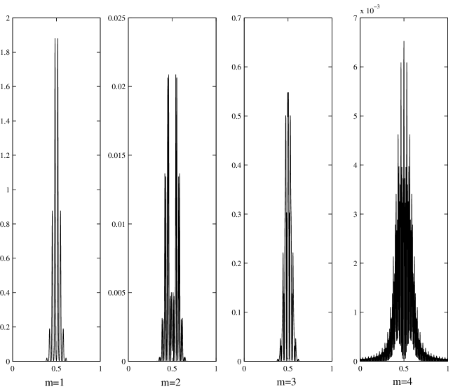
Fig. 1: $|\mathbb{P}^{\varepsilon}_{m}\psi_{\rm in}|^{2}$, $m=1,\cdots,4$ for ${\varepsilon}=\frac{1}{32}$.

Since $\psi_{\rm in}$ is smooth we expect that only very few bands have to be taken into account in the Bloch decomposition. Indeed we observe that the amount of mass corresponding to $\mathbb{P}^{\varepsilon}_{m}\psi_{\rm in}$, i.e. the mass concentration in each Bloch band, decays rapidly as $m\to\infty$, see Table 1. In other words, the number $M_{0}$ is essentially determined by the regularity of $\psi_{\rm in}$ in each cell. Note that $M_{0}$ is independent of ${\varepsilon}$.

Table 1: The values of $\mathrm{M}_{m}^{\varepsilon}:={\big{\|}\,\mathbb{P}^{\varepsilon}_{m}\psi_{\rm in}\big{\|}}_{L^{2}({\mathbb{R}})}$, for ${\varepsilon}=\frac{1}{32}$:

$m$	1	2	3	4
${\mathrm{M}}^{\varepsilon}_{m}$	$7.91\rm{E}-1$	$1.11\rm{E}-1$	$5.92\rm{E}-1$	$8.80\rm{E}-2$
$m$	5	6	7	8
${\mathrm{M}}^{\varepsilon}_{m}$	$8.67\rm{E}-2$	$2.81\rm{E}-3$	$2.80\rm{E}-3$	$4.98\rm{E}-5$

To compute the evolution of these initial data we shall take into account $M\geq M_{0}$ bands. Note that only in cases where $U(x)\equiv 0$ one can take $M$ to be identical to $M_{0}$, the initial band cut-off. The reason is that if $U(x)$ is nonzero Step 2 in the BD algorithm given above mixes all bands. In particular all the $\psi_{m}(t)$ are no longer orthogonal to each other. Roughly speaking however, if ${\varepsilon}$ is very small, all band spaces $\mathcal{H}_{m}$ remain “almost orthogonal” and thus the mass within each Bloch band, i.e. $\mathrm{M}_{m}^{\varepsilon}(t):={\big{\|}\,\mathbb{P}^{\varepsilon}_{m}\psi(t)\big{\|}}^{2}_{L^{2}({\mathbb{R}})}$ is “almost conserved”. More precisely it is conserved up to errors $\mathcal{O}({\varepsilon})$ on time scales $\mathcal{O}(1)$. Thus, by checking mass conservation after each time step one gets a rather reliable measure on the amount of mixing of the bands. In other words if the mass conservation after some time steps gets worse, one has to take into account more bands to proceed.

We find numerically that the use of $M=M_{0}\approx 8$ bands already yields satisfactory results for ${\varepsilon}=\frac{1}{32}$. In the following though we shall even compute $M=32$ energy bands, which is by far sufficient for our purposes (even if ${\varepsilon}=\frac{1}{2}$). Note that the number of required bands $M$ depends on the regularity properties of $U(x)$, as well as on the considered time-scales (which might be even longer than $\mathcal{O}(1)$, the case considered here). This approximation problem is more or less analogous to the one appearing in spectral schemes for PDEs with non-smooth coefficients.

Concerning slowly varying, external potentials $U$, we shall choose, on the one hand, smooth functions which are either of the form

(4.2) $$U(x)=\mathcal{E}x,$$

modelling a constant (electric) force field $\mathcal{E}\in{\mathbb{R}}$, or given by a harmonic oscillator type potential

(4.3) $$U(x)=|x-\pi|^{2}.$$

On the other hand, we shall also consider the case of an external (non-smooth) step potential, i.e.

(4.4) $$U(x)=\left\{\begin{array}[]{ll}1,&x\in\left[\frac{\pi}{2},\frac{3\pi}{2}\right]\\ 0,&\mbox{else}.\end{array}\right.$$

Within the setting described above, we shall focus on two particular choices for the lattice potential, namely:

Example 4.1 (Mathieu’s model).

The so-called Mathieu’s model, i.e.

(4.5) $$V_{\Gamma}(x)=\cos(x),$$

as already considered in [19]. (For applications in solid state physics this is rather unrealistic, however it fits quite good with experiments on Bose-Einstein condensates in optical lattices.) In this case all Fourier coefficients $\widehat{V}(\lambda)$, appearing in (2.19) are zero, except for $\widehat{V}(\pm 1)=\frac{1}{2}$ and thus ${\mathbf{H}}(k)$, given in (2.30), simplifies to a tri-diagonal matrix.

Example 4.2 (Kronig-Penney’s model).

The so-called Kronig-Penney’s model, i.e.

(4.6) $$V_{\Gamma}(x)=1-\sum_{\gamma\in{\mathbb{Z}}}{\bf 1}_{x\in\left[\frac{\pi}{2}+2\pi\gamma,\frac{3\pi}{2}+2\pi\gamma\right]},$$

where ${\bf 1}_{\Omega}$ denotes the characteristic function of a set $\Omega\subset{\mathbb{R}}$. In contrast to Mathieu’s model this case comprises a non-smooth lattice potential. The corresponding Bloch eigenvalue problem is known to be explicitly solvable (see, e.g., [19]).

In order to compare the different numerical algorithms we denote by $\psi^{\rm ts}(t,x)$ the solution gained from the time-splitting spectral method, whereas $\psi^{\rm bd}(t,x)$ denotes the solution obtained via the new method base on Bloch’s decomposition. Both methods will be compared to the “exact” solution $\psi^{\rm ex}(t,x)$, which is obtained using a very fine spatial grid. We consider the following errors

(4.7) $$\Delta^{\rm bd/ts}_{\infty}(t):= \,{\big{\|}\,\psi^{\rm ex}(t,\cdot)-\psi^{\rm bd/ts}(t,\cdot)\big{\|}}_{L^{\infty}({\mathbb{R}})},$$

$$\Delta^{\rm bd/ts}_{2}(t):= \,{\big{\|}\,\psi^{\rm ex}(t,\cdot)-\psi^{\rm bd/ts}(t,\cdot)\big{\|}}_{L^{2}({\mathbb{R}})}$$

between the “exact solution” and the corresponding solutions obtained via the Bloch decomposition based algorithm resp. the classical time splitting spectral method. The numerical experiments are now done in a series of three different settings:

• First we shall study both cases of $V_{\Gamma}$, imposing additionally $U(x)\equiv 0$, i.e. no external potential. The obtained results are given in Table 3, where ${\varepsilon}=\frac{1}{2}$, $\frac{1}{32}$, and $\frac{1}{1024}$, respectively. In the last case the oscillations are extremely spurious. As discussed before, we can use only one step in time to obtain the numerical solution, because the Bloch-decomposition method indeed is “exact” in this case (independently of ${\varepsilon}$). Thus, even if we would refine the time steps in the BD algorithm we would not get more accurate approximations. On the other hand, by using the usual time-splitting method, one has to refine the time steps (depending on ${\varepsilon}$) as well as the mesh size in order to achieve the same accuracy. More precisely we find that $\Delta t=\mathcal{O}({\varepsilon})$, $\Delta x=\mathcal{O}({\varepsilon}^{\alpha})$, for some $\alpha\geq 1$, is needed when using TS (see also the computations given in [19]). In particular $\alpha>1$ is required for the case of a non-smooth lattice potential $V_{\Gamma}$. (Note that if $V_{\Gamma}=0$ it is well known that $\Delta x=\mathcal{O}({\varepsilon})$, is sufficient, cf. [3, 4, 24]).

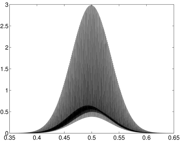
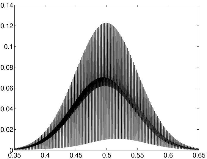
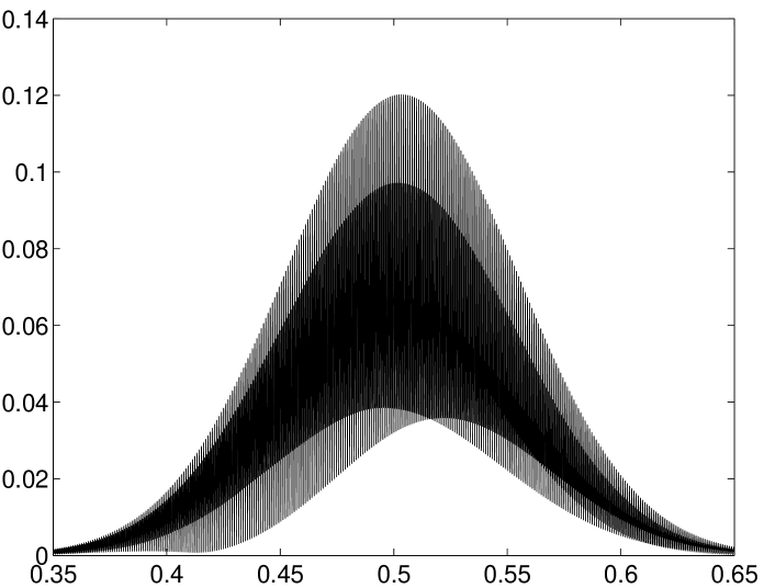
$|\psi^{\rm ex}(t,x)|^{2}$, $|\psi^{\rm ex}(t,x)-\psi^{\rm ts}(t,x)|$ and $|\psi^{\rm ex}(t,x)-\psi^{\rm bd}(t,x)|$ at $t=0.1$

Fig. 4: Numerical results for example 4.1 with $U(x)$ given by (4.2) and ${\varepsilon}=\frac{1}{1024}$. We use $\triangle t=\frac{1}{5000}$, $\triangle x=\frac{1}{16384}$ for the TS, $\triangle t=\frac{1}{20}$, $\triangle x=\frac{1}{8192}$ for the BD method, and $\triangle t=\frac{1}{100000}$, $\triangle x=\frac{1}{131072}$ for the “exact” solution.

• In a second series of numerical experiments we shall consider only Example 4.1 for the periodic potential but taking into account all three cases of the external potentials $U$, as given above. In Fig. 4–8, we show the obtained numerical results for ${\varepsilon}=\frac{1}{2}$, and ${\varepsilon}=\frac{1}{1024}$, respectively. We observe that, if ${\varepsilon}=\mathcal{O}(1)$, the Bloch-decomposition method gives almost the same results as time-splitting spectral method. However, if ${\varepsilon}\ll 1$, we can achieve quite good accuracy by using the Bloch-decomposition method with $\Delta t=\mathcal{O}(1)$ and $\Delta x=\mathcal{O}({\varepsilon})$. On the other hand, using the standard TS algorithm, we again have to rely on much finer spatial grids and time steps to achieve the same accuracy.

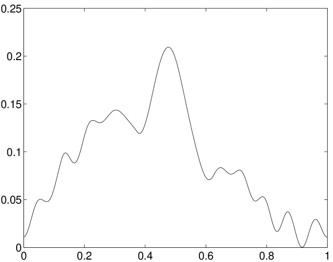
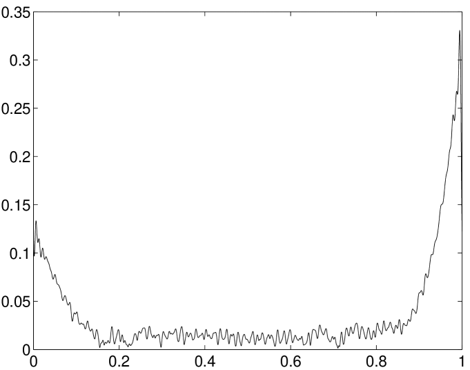
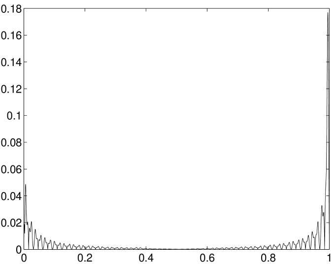
$|\psi^{\rm ex}(t,x)|^{2}$, $|\psi^{\rm ex}(t,x)-\psi^{\rm ts}(t,x)|$ and $|\psi^{\rm ex}(t,x)-\psi^{\rm bd}(t,x)|$ at $t=1.0$

Fig. 9: Numerical results for example 4.2 with $U(x)$ given by (4.2), ${\varepsilon}=\frac{1}{2}$. We use $\triangle t=\frac{1}{100}$, $\triangle x=\frac{1}{64}$ for the TS, $\triangle t=\frac{1}{2}$, $\triangle x=\frac{1}{32}$ for BD method, and $\triangle t=\frac{1}{100000}$, $\triangle x=\frac{1}{8192}$ for the “exact” solution.

$$\Delta^{\rm ts}_{\infty}(t)=3.31\rm{E}-1,\ \Delta^{\rm bd}_{\infty}(t)=1.77\rm{E}-1,\ \Delta^{\rm ts}_{2}(t)=6.16\rm{E}-2,\ \Delta^{\rm bd}_{2}(t)=1.38\rm{E}-2.$$

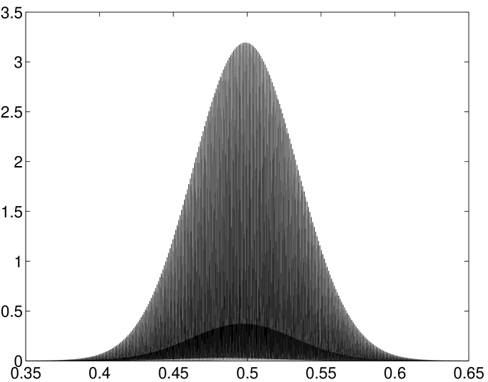
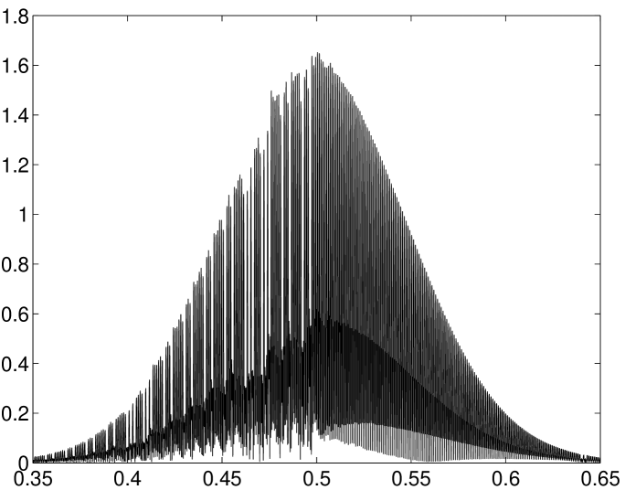
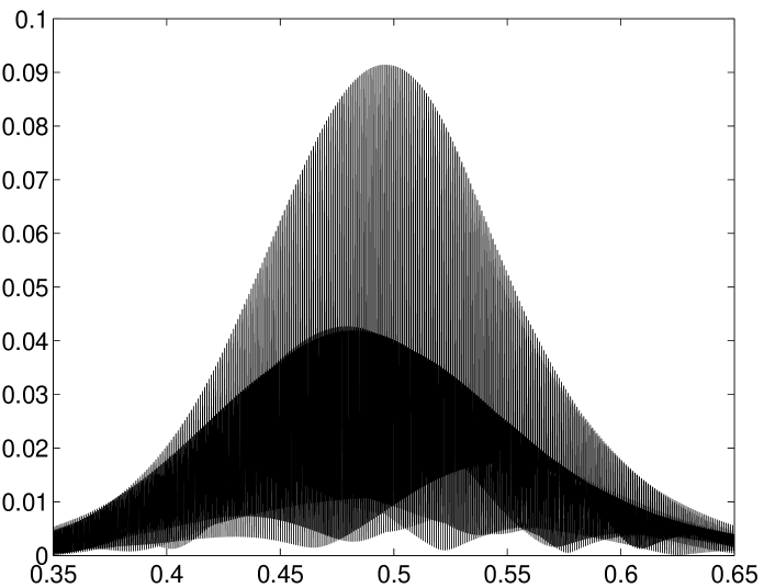
$|\psi^{\rm ex}(t,x)|^{2}$, $|\psi^{\rm ex}(t,x)-\psi^{\rm ts}(t,x)|$ and $|\psi^{\rm ex}(t,x)-\psi^{\rm bd}(t,x)|$ at $t=0.1$

Fig. 10: Numerical results for example 4.2 with $U(x)$ given by (4.2), ${\varepsilon}=\frac{1}{1024}$. We use $\triangle t=\frac{1}{10000}$, $\triangle x=\frac{1}{65536}$ for the TS, $\triangle t=\frac{1}{10}$, $\triangle x=\frac{1}{8192}$ for the BD method, and $\triangle t=\frac{1}{100000}$, $\triangle x=\frac{1}{131072}$ for the “exact” solution.

• We finally show the numerical results obtained by combining external fields and a non-smooth lattice potential given by Example 4.2. As before we include all three cases for the external potential $U$. The cases ${\varepsilon}=\frac{1}{2}$, and $\frac{1}{1024}$ are studied and the obtained results are given in Fig. 10–14, respectively. We observe that the results of the Bloch-decomposition are much better than the time-splitting spectral method, even if ${\varepsilon}=\frac{1}{2}$. Moreover, as ${\varepsilon}$ gets smaller, the advantages of the Bloch-decomposition method are even better visible.

To convince ourselves that only a few Bloch bands contribute to $\|\psi\|_{L^{2}({\mathbb{R}})}$, even after time steps $\mathcal{O}(1)$, we show in the following table the numerical values of $\mathrm{M}^{\varepsilon}_{m}(t)={\big{\|}\,\mathbb{P}^{\varepsilon}_{m}\psi(t)\big{\|}}^{2}_{L^{2}({\mathbb{R}})}$, for $m=1,\cdots,8$, corresponding to the solution of Example 4.1 with $U$ given by (4.3).

Table 2: The mass of $\psi(t,x)$, solution to Example 4.1 with external potential (4.3), decomposed into the Bloch bands for ${\varepsilon}=\frac{1}{32}$ at time $t=1$:

$m$	1	2	3	4
$\mathrm{M}_{m}^{\varepsilon}$	$7.89\rm{E}-1$	$1.10\rm{E}-2$	$5.92\rm{E}-1$	$9.38\rm{E}-2$
$m$	5	6	7	8
$\mathrm{M}_{m}^{\varepsilon}$	$7.15\rm{E}-2$	$3.50\rm{E}-3$	$1.80\rm{E}-3$	$5.63\rm{E}-5$

We also check the conservation of the total (discrete) mass, i.e. ${\|\psi(t)\|}_{l^{2}(\mathcal{D})}$. We find that numerically it is of the order $10^{-6}$ for the smooth lattice potential (4.5) and $10^{-3}$ for the non-smooth case (4.6). The latter however can be improved by using a refined spatial grid and more time steps.

In summary we find (at least for our one dimensional computations) that, relying on the new Bloch-decomposition based algorithm, one can use much larger time steps, and sometimes even a coarser spatial grid, to achieve the same accuracy as for the usual time-splitting spectral method. This is particularly visible in cases, where the lattice potential is non longer smooth and ${\varepsilon}\ll 1$. Indeed in these cases the BD algorithm turns out to be considerably faster than the TS method.

Remark 4.1.

In view of our results the earlier numerical studies based on TS methods [19, 18, 20], should be taken with some care, in particular when comparing the full Schrödinger solution to the semiclassical approximation beyond caustics.

Table 3: The results of Example 4.1 with $U(x)=0$:

Spatial discretization error test at time $t=1.0$ for ${\varepsilon}=1/2$.
For TS $\triangle t=0.0001$ and for BD $\triangle t=1$. mesh size $\triangle x/{\varepsilon}$ $1/2$ $1/4$ $1/8$ $1/16$ $\begin{array}[]{c}\vspace*{-4mm}\hfil\\ \left\|\psi^{\rm ts}_{\triangle x,\triangle t}(t,\cdot)-\psi^{\rm ex}(t,\cdot)\right\|_{l^{2}}\\ \vspace*{-4mm}\hfil\end{array}$ 4.33E-1 2.53E-1 2.80E-2 6.42E-6 convergence order 0.8 3.2 12.1 $\begin{array}[]{c}\vspace*{-4mm}\hfil\\ \left\|\psi^{\rm bd}_{\triangle x,\triangle t}(t,\cdot)-\psi^{\rm ex}(t,\cdot)\right\|_{l^{2}}\\ \vspace*{-4mm}\hfil\end{array}$ 3.01E-1 1.95E-1 1.39E-2 1.17E-6 convergence order 0.6 3.8 13.5

Spatial discretization error test at time $t=0.1$ for ${\varepsilon}=1/32$.
For TS $\triangle t=0.00001$ and for BD $\triangle t=0.1$. mesh size $\triangle x/{\varepsilon}$ $1/2$ $1/4$ $1/8$ $1/16$ $\begin{array}[]{c}\vspace*{-4mm}\hfil\\ \left\|\psi^{\rm ts}_{\triangle x,\triangle t}(t,\cdot)-\psi^{\rm ex}(t,\cdot)\right\|_{l^{2}}\\ \vspace*{-4mm}\hfil\end{array}$ 2.88E-1 1.08E-1 9.63E-4 1.33E-7 convergence order 1.4 6.8 12.8 $\begin{array}[]{c}\vspace*{-4mm}\hfil\\ \left\|\psi^{\rm bd}_{\triangle x,\triangle t}(t,\cdot)-\psi^{\rm ex}(t,\cdot)\right\|_{l^{2}}\\ \vspace*{-4mm}\hfil\end{array}$ 2.53E-1 7.34E-2 8.97E-4 4.95E-10 convergence order 1.8 6.4 20.8

Spatial discretization error test at time $t=0.01$ for ${\varepsilon}=1/1024$.
For TS $\triangle t=0.000001$ and for BD $\triangle t=0.01$. mesh size $\triangle x/{\varepsilon}$ $1/2$ $1/4$ $1/8$ $1/16$ $\begin{array}[]{c}\vspace*{-4mm}\hfil\\ \left\|\psi^{\rm ts}_{\triangle x,\triangle t}(t,\cdot)-\psi^{\rm ex}(t,\cdot)\right\|_{l^{2}}\\ \vspace*{-4mm}\hfil\end{array}$ 5.14E-1 1.94E-1 1.08E-3 6.08E-8 convergence order 1.4 7.5 14.1 $\begin{array}[]{c}\vspace*{-4mm}\hfil\\ \left\|\psi^{\rm bd}_{\triangle x,\triangle t}(t,\cdot)-\psi^{\rm ex}(t,\cdot)\right\|_{l^{2}}\\ \vspace*{-4mm}\hfil\end{array}$ 2.64E-1 6.83E-2 2.29E-4 1.71E-10 convergence order 2.0 8.2 20.4

Table 4: The results of Example 4.1 with linear external potential (4.2):

Spatial discretization error test at time $t=0.1$ for ${\varepsilon}=1/2$.
For TS $\triangle t=0.0001$ and for BD $\triangle t=0.01$. mesh size $\triangle x/{\varepsilon}$ $1/2$ $1/4$ $1/8$ $1/16$ $\begin{array}[]{c}\vspace*{-4mm}\hfil\\ \left\|\psi^{\rm ts}_{\triangle x,\triangle t}(t,\cdot)-\psi^{\rm ex}(t,\cdot)\right\|_{l^{2}}\\ \vspace*{-4mm}\hfil\end{array}$ 2.73E-1 9.22E-2 5.78E-3 4.73E-6 convergence order 1.6 4.0 10.3 $\begin{array}[]{c}\vspace*{-4mm}\hfil\\ \left\|\psi^{\rm bd}_{\triangle x,\triangle t}(t,\cdot)-\psi^{\rm ex}(t,\cdot)\right\|_{l^{2}}\\ \vspace*{-4mm}\hfil\end{array}$ 3.15E-1 1.55E-1 1.32E-2 3.36E-6 convergence order 1.0 3.6 11.9

Spatial discretization error test at time $t=0.01$ for ${\varepsilon}=1/1024$.
For TS $\triangle t=0.00001$ and for BD $\triangle t=0.001$. mesh size $\triangle x/{\varepsilon}$ $1/2$ $1/4$ $1/8$ $1/16$ $\begin{array}[]{c}\vspace*{-4mm}\hfil\\ \left\|\psi^{\rm ts}_{\triangle x,\triangle t}(t,\cdot)-\psi^{\rm ex}(t,\cdot)\right\|_{l^{2}}\\ \vspace*{-4mm}\hfil\end{array}$ 5.22E-1 1.98E-1 1.53E-2 3.19E-5 convergence order 1.4 3.7 8.9 $\begin{array}[]{c}\vspace*{-4mm}\hfil\\ \left\|\psi^{\rm bd}_{\triangle x,\triangle t}(t,\cdot)-\psi^{\rm ex}(t,\cdot)\right\|_{l^{2}}\\ \vspace*{-4mm}\hfil\end{array}$ 4.71E-1 1.61E-1 9.17E-3 6.08E-6 convergence order 1.5 4.1 10.6

Temporal discretization error test at $t=0.1$ for ${\varepsilon}=1/2$ and $\triangle x/{\varepsilon}=1/128$. time step $\triangle t$ $1/10$ $1/20$ $1/40$ $1/80$ $\begin{array}[]{c}\vspace*{-4mm}\hfil\\ \left\|\psi^{\rm ts}_{\triangle x,\triangle t}(t,\cdot)-\psi^{\rm ex}(t,\cdot)\right\|_{l^{2}}\\ \vspace*{-4mm}\hfil\end{array}$ 2.59E-4 6.47E-5 1.62E-5 4.04E-6 convergence order 2.0 2.0 2.0 $\begin{array}[]{c}\vspace*{-4mm}\hfil\\ \left\|\psi^{\rm bd}_{\triangle x,\triangle t}(t,\cdot)-\psi^{\rm ex}(t,\cdot)\right\|_{l^{2}}\\ \vspace*{-4mm}\hfil\end{array}$ 4.86E-5 1.23E-5 3.08E-6 7.60E-7 convergence order 2.0 2.0 2.0

Temporal discretization error test at $t=0.01$ for ${\varepsilon}=1/1024$ and $\triangle x/{\varepsilon}=1/128$. time step $\triangle t$ $1/1000$ $1/2000$ $1/4000$ $1/8000$ $\begin{array}[]{c}\vspace*{-4mm}\hfil\\ \left\|\psi^{\rm ts}_{\triangle x,\triangle t}(t,\cdot)-\psi^{\rm ex}(t,\cdot)\right\|_{l^{2}}\\ \vspace*{-4mm}\hfil\end{array}$ 6.60E-2 1.54E-2 3.81E-3 9.45E-4 convergence order 2.1 2.0 2.0 time step $\triangle t$ $1/100$ $1/200$ $1/400$ $1/800$ $\begin{array}[]{c}\vspace*{-4mm}\hfil\\ \left\|\psi^{\rm bd}_{\triangle x,\triangle t}(t,\cdot)-\psi^{\rm ex}(t,\cdot)\right\|_{l^{2}}\\ \vspace*{-4mm}\hfil\end{array}$ 3.32E-3 7.54E-4 1.42E-4 3.16E-5 convergence order 2.1 2.4 2.2

Table 5: The results of Example 4.2 with harmonic external potential (4.3):

Spatial discretization error test at time $t=0.1$ for ${\varepsilon}=1/2$.
For TS $\triangle t=0.0001$ and for BD $\triangle t=0.01$. mesh size $\triangle x/{\varepsilon}$ $1/2$ $1/4$ $1/8$ $1/16$ $\begin{array}[]{c}\vspace*{-4mm}\hfil\\ \left\|\psi^{\rm ts}_{\triangle x,\triangle t}(t,\cdot)-\psi^{\rm ex}(t,\cdot)\right\|_{l^{2}}\\ \vspace*{-4mm}\hfil\end{array}$ 2.71E-1 8.87E-2 5.19E-3 1.32E-4 convergence order 1.6 4.1 5.3 $\begin{array}[]{c}\vspace*{-4mm}\hfil\\ \left\|\psi^{\rm bd}_{\triangle x,\triangle t}(t,\cdot)-\psi^{\rm ex}(t,\cdot)\right\|_{l^{2}}\\ \vspace*{-4mm}\hfil\end{array}$ 3.23E-1 9.08E-2 7.03E-3 1.27E-4 convergence order 1.8 3.7 5.8

Spatial discretization error test at time $t=0.01$ for ${\varepsilon}=1/1024$.
For TS $\triangle t=0.00001$ and for BD $\triangle t=0.001$. mesh size $\triangle x/{\varepsilon}$ $1/2$ $1/4$ $1/8$ $1/16$ $\begin{array}[]{c}\vspace*{-4mm}\hfil\\ \left\|\psi^{\rm ts}_{\triangle x,\triangle t}(t,\cdot)-\psi^{\rm ex}(t,\cdot)\right\|_{l^{2}}\\ \vspace*{-4mm}\hfil\end{array}$ 3.99E-1 3.67E-1 2.19E-1 1.10E-1 convergence order 0.1 0.7 1.0 $\begin{array}[]{c}\vspace*{-4mm}\hfil\\ \left\|\psi^{\rm bd}_{\triangle x,\triangle t}(t,\cdot)-\psi^{\rm ex}(t,\cdot)\right\|_{l^{2}}\\ \vspace*{-4mm}\hfil\end{array}$ 2.06E-1 5.64E-2 8.16E-3 6.40E-4 convergence order 1.9 2.8 3.7

Temporal discretization error test at $t=0.1$ for ${\varepsilon}=1/2$ and $\triangle x/{\varepsilon}=1/128$. time step $\triangle t$ $1/10$ $1/20$ $1/40$ $1/80$ $\begin{array}[]{c}\vspace*{-4mm}\hfil\\ \left\|\psi^{\rm ts}_{\triangle x,\triangle t}(t,\cdot)-\psi^{\rm ex}(t,\cdot)\right\|_{l^{2}}\\ \vspace*{-4mm}\hfil\end{array}$ 1.02E-3 6.41E-4 3.80E-4 2.18E-4 convergence order 0.7 0.8 0.8 $\begin{array}[]{c}\vspace*{-4mm}\hfil\\ \left\|\psi^{\rm bd}_{\triangle x,\triangle t}(t,\cdot)-\psi^{\rm ex}(t,\cdot)\right\|_{l^{2}}\\ \vspace*{-4mm}\hfil\end{array}$ 4.20E-6 1.02E-6 2.22E-7 5.56E-8 convergence order 2.0 2.2 2.0

Temporal discretization error test at $t=0.01$ for ${\varepsilon}=1/1024$ and $\triangle x/{\varepsilon}=1/128$. time step $\triangle t$ $1/1000$ $1/2000$ $1/4000$ $1/8000$ $\begin{array}[]{c}\vspace*{-4mm}\hfil\\ \left\|\psi^{\rm ts}_{\triangle x,\triangle t}(t,\cdot)-\psi^{\rm ex}(t,\cdot)\right\|_{l^{2}}\\ \vspace*{-4mm}\hfil\end{array}$ 1.21E-1 1.18E-1 1.10E-1 1.10E-1 convergence order 0.04 0.1 0.0 time step $\triangle t$ $1/100$ $1/200$ $1/400$ $1/800$ $\begin{array}[]{c}\vspace*{-4mm}\hfil\\ \left\|\psi^{\rm bd}_{\triangle x,\triangle t}(t,\cdot)-\psi^{\rm ex}(t,\cdot)\right\|_{l^{2}}\\ \vspace*{-4mm}\hfil\end{array}$ 3.30E-5 5.21E-6 1.23E-6 3.16E-7 convergence order 2.6 2.1 2.0

5 Asymptotic analysis in the semiclassical regime

For completeness we shall also compare the numerical solution of the Schrödinger equation (1.1) with its semiclassical asymptotic description. To this end we shall rely on a multiple scales WKB-type expansion methods, even though there are currently more advanced tools at hand, cf. [17, 30, 32]. The WKB method however has the advantage of given a rather simple and transparent description of $\psi(t)$, solution to (1.1), for ${\varepsilon}\ll 1$, (at least locally in-time). Since the Bloch decomposition method itself is rather abstract we include this approximative description here too, so that the reader gets a better feeling for the appearing quantities. Moreover this two-scale WKB method can also be used for nonlinear Schrödinger dynamics [12], a problem we shall study numerically in an upcoming work.

5.1 The WKB formalism

To this end let us suppose that the initial condition is of (two-scale) WKB-type. More precisely assume

(5.1) $$\psi_{\rm in}(x)=\sum^{M}_{m=1}u_{m}\left(x,\frac{x}{{\varepsilon}}\right)\,\mathrm{e}^{i\phi(x)/{\varepsilon}},$$

with some given real-valued phase $\phi\in C^{\infty}({\mathbb{R}})$ and some given initial (complex-valued) band-amplitudes $u_{m}(x,y+2\pi)=u_{m}(x,y)$, each of which admits an asymptotic description of the following form

(5.2) $$u_{m}(x,y)\sim{u}^{0}_{m}\left(x,y\right)+{\varepsilon}{u}^{1}_{m}\left(x,y\right)+\mathcal{O}({\varepsilon}^{2})\quad\forall\,m\in{\mathbb{N}}.$$

Here and in the following we shall only be concerned with the leading order asymptotic description.

Remark 5.1.

Note that we do consider only a single initial WKB-phase $\phi(x)$ for all bands $m\in{\mathbb{N}}$. We could of course also allow for more general cases, like one WKB-phase for each band or even a superposition of WKB-states within each band. However in order to keep the presentation clean we hesitate to do so. The standard WKB approximation, for non-periodic problems, involves real-valued amplitudes $\tilde{u}^{0}(x),\tilde{u}^{1}(x),\dots$ which only depend on the slow scale.

It is well known then, cf. [12, 21], that the leading order term ${u}^{0}_{m}$, $m\in{\mathbb{N}}$, can be decomposed as

(5.3) $${u}^{0}_{m}\left(x,\frac{x}{{\varepsilon}}\right)=f_{m}(x)\chi_{m}\left(\frac{x}{{\varepsilon}},\partial_{x}\phi(x)\right),$$

where we assume the m-th energy band to be non-degenerated (for simplicity) and isolated from the rest of spectrum. We can choose an arbitrary $f_{m}\in\mathcal{S}({\mathbb{R}})$. In other words, there is an adiabatic decoupling between the slow scale $x$ and fast scale $x/{\varepsilon}$. Indeed, a lengthy calculation, invoking the classical stationary phase argument, cf. chapter 4.7 in [7], shows that in this case the band projection $\mathbb{P}^{\varepsilon}_{m}\psi$ can be approximated via

(5.4) $$\mathbb{P}_{m}^{\varepsilon}\psi(x)\sim f_{m}(x)\,\chi_{m}\left(\frac{x}{{\varepsilon}},\partial_{x}\phi(x)\right)\mathrm{e}^{i\phi(x)/{\varepsilon}}+\mathcal{O}({\varepsilon}).$$

This approximate formula shows the origin of the high oscillations induced either by $V_{\Gamma}$, described by $\chi_{m}$, or by the dispersion, described by $\phi(x)$. We note that in general the higher order terms (in ${\varepsilon}$), such as $u^{1}_{m}$ etc., are of a more complicated structure than (5.3), but we shall neglect these terms in what follows (see, e.g., [12] for more details). One consequently finds that $\psi(t)$ obeys a leading order asymptotic description of the form

(5.5) $$\psi(t,x)\sim\sum_{m=1}^{M}a_{m}(t,x)\,\chi_{m}\left(\frac{x}{{\varepsilon}},\partial_{x}\phi_{m}(t,x)\right)\mathrm{e}^{i\phi_{m}(t,x)/{\varepsilon}}+\mathcal{O}({\varepsilon}),$$

where $\phi_{m}(t,x)\in C^{\infty}([0,t_{c})\times{\mathbb{R}})$ satisfies the $m$th band Hamilton-Jacobi equation

(5.6) $$\left\{\begin{aligned} &\partial_{t}\phi_{m}(t,x)+E_{m}(\partial_{x}\phi_{m})+U(x)=\,0,\quad m\in{\mathbb{N}},\\ &\phi_{m}\big{|}_{t=0}=\,\phi(x).\end{aligned}\right.$$

Also, the (complex-valued) leading order WKB-amplitude $a_{m}(t,x)\in C^{\infty}([0,t_{c})\times{\mathbb{R}})$ satisfies the following semiclassical transport equations

(5.7) $$\left\{\begin{aligned} &\partial_{t}a_{m}+\partial_{k}E_{m}(\partial_{x}\phi_{m})\partial_{x}a_{m}+\frac{1}{2}\,\partial_{x}(\partial_{k}E_{m}(\partial_{x}\phi_{m}))a_{m}-(\beta_{m}(t,x)\partial_{x}U(x))\,a_{m}=0,\\ &a_{m}\big{|}_{t=0}=f_{m}(x).\end{aligned}\right.$$

with $\beta_{m}(t,x):={\langle\chi_{m}(y,k),\partial_{k}\chi_{m}(y,k)\rangle}_{L^{2}(\mathcal{C})}$, evaluated at $k=\partial_{x}\phi_{m}$, the so-called Berry phase term.

Remark 5.2.

Note that the Berry term is purely imaginary, i.e. $\beta_{m}(t,x)\in\mathrm{i}{\mathbb{R}}$, which implies the following conservation law

(5.8) $$\partial_{t}|a_{m}|^{2}+\partial_{x}\left(\partial_{k}E_{m}(\partial_{x}\phi_{m})|a_{m}|^{2}\right)=0\quad\forall\,m\in{\mathbb{N}}.$$

Of course the above given WKB-type expansion method is only valid up to the (in general finite) time $0\leq t_{\rm c}<\infty$, the caustic onset-time in the solution of (5.6). Here we shall simply assume that $t_{c}>0$ holds, i.e. no caustic is formed at time $t=0$, which is very well possible in general. We note that in the considered numerical examples below we indeed have $t_{c}>0$ and we refer to [11] for a broader discussion on this. For $t\geq t_{\rm c}$ one would need to superimpose several WKB-type solutions corresponding to the multi-valued solutions of the flow map $(x,t)\mapsto X_{t}(x)\equiv X_{t}(x;\partial_{x}\phi(x))$, where

(5.9) $$\left\{\begin{aligned} \dot{X}_{t}=&\ \partial_{k}E_{m}(\Xi_{t}),\quad X_{0}=x,\\ \dot{\Xi}_{t}=&\ -\partial_{x}U(X_{t}),\quad\Xi_{0}=\partial_{x}\phi(x).\end{aligned}\right.$$

Numerically we shall use the relaxation method introduced in [25] to solve the Hamilton-Jacobi equation (5.6). Consequently we can solve the system of transport equations (5.7) by a time-splitting spectral scheme similar to the ones used above.

5.2 Numerical examples

We shall finally study the WKB approach, briefly described above, by some numerical examples. Denote by

(5.10) $$\psi^{\rm sc}(t,x):=\sum_{m=1}^{M}f_{m}(t,x)\chi_{m}\left(\frac{x}{{\varepsilon}},\partial_{x}\phi_{m}\right)e^{i\phi_{m}(t,x)/{\varepsilon}},$$

the approximate semiclassical solution to the Schrödinger equation (1.1). In the following examples we only take into account a harmonic external potential of the form (4.3).

Example 5.1 (Mathieu’s model).

We first consider Mathieu’s model (4.5) and choose initial condition in the form

(5.11) $$\psi_{\rm in}(x)=\mathrm{e}^{-5(x-\pi)^{2}}\chi_{1}\left(\frac{x}{{\varepsilon}},0\right),$$

i.e. we choose $\phi(x)=0$ and restrict ourselves to the case of only one band with index $m=1$. (Since $E_{1}(k)$ is an isolated band the analytical results of [7, 12, 21], then imply that we can neglect the contributions from all other bands $m>1$ up to errors of order $\mathcal{O}({\varepsilon})$ in $L^{2}({\mathbb{R}})\cap L^{\infty}({\mathbb{R}})$, uniformly on compact time-intervals.) In this case, we numerically find that no caustic is formed within the solution of (5.6) at least up to $t=1$, the largest time in our computation. Note that (5.11) concentrates at the minimum of the first Bloch band, where it is known that

(5.12) $$E_{m}(k)\approx\frac{|k|^{2}}{2m^{*}}+E_{m}(0),$$

This is the so-called parabolic band approximation, yielding an effective mass $m^{*}\in{\mathbb{R}}$. In Table 6, we show the results with an additional harmonic external potential, cf. (4.3), for ${\varepsilon}=\frac{1}{32}$ and ${\varepsilon}=\frac{1}{1024}$ respectively.

Table 6: Difference between the asymptotic solution and the Schrödinger equation for example 5.1 ($\triangle t=10^{-4}$, $\triangle x=1/32768$):

${\varepsilon}$	$\frac{1}{32}$	$\frac{1}{1024}$
$\begin{array}[]{c}\vspace{-4mm}\hfil\\ \displaystyle\sup_{0\leq t\leq 1}\left\|\,\psi(t,x)-\psi^{\rm sc}(t,x)\,\right\|_{L^{2}({\mathbb{R}})}\end{array}$	$6.68\rm{E}-3$	$3.08\rm{E}-4$
$\begin{array}[]{c}\vspace{-4mm}\hfil\\ \displaystyle\sup_{0\leq t\leq 1}\left\|\,\psi(t,x)-\psi^{\rm sc}(t,x)\,\right\|_{L^{\infty}({\mathbb{R}})}\end{array}$	$5.57\rm{E}-2$	$2.38\rm{E}-3$

Note that these numerical experiments, together with those given below, confirm the analytical results given in [7, 12, 21].

Example 5.2 (Kronig-Penney’s model).

Here, we consider again the Kronig-Penney’s model (4.6). First we use the same initial condition as given in (5.11) but with $m=2$, which again corresponds to an isolated energy band. The corresponding numerical results for ${\varepsilon}=\frac{1}{32}$ and $\frac{1}{1024}$ are shown in Table 7.

Table 7: Difference between the asymptotic solution and the Schrödinger equation for example 5.2 for initial condition (5.11) ($\triangle t=10^{-4}$, $\triangle x=1/32768$):

${\varepsilon}$	$\frac{1}{32}$	$\frac{1}{1024}$
$\begin{array}[]{c}\vspace{-4mm}\hfil\\ \displaystyle\sup_{0\leq t\leq 0.1}\left\|\,\psi(t,x)-\psi^{\rm sc}(t,x)\,\right\|_{L^{2}({\mathbb{R}})}\end{array}$	$1.18\rm{E}-2$	$1.08\rm{E}-3$
$\begin{array}[]{c}\vspace{-4mm}\hfil\\ \displaystyle\sup_{0\leq t\leq 0.1}\left\|\,\psi(t,x)-\psi^{\rm sc}(t,x)\,\right\|_{L^{\infty}({\mathbb{R}})}\end{array}$	$9.34\rm{E}-2$	$7.74\rm{E}-3$

In a second case, we alternatively choose initial data of the form

(5.13) $$\psi_{\rm in}(x)=\mathrm{e}^{-5(x-\pi)^{2}}\chi_{2}\left(\frac{x}{{\varepsilon}},\sin(x)\right)\mathrm{e}^{-\mathrm{i}\cos(x)/{\varepsilon}},$$

i.e. $\phi(x)=-\cos(x)$. Here we find (numerically) that the caustic onset time is roughly given by $t_{c}\approx 0.24$, cf. Fig. 2.

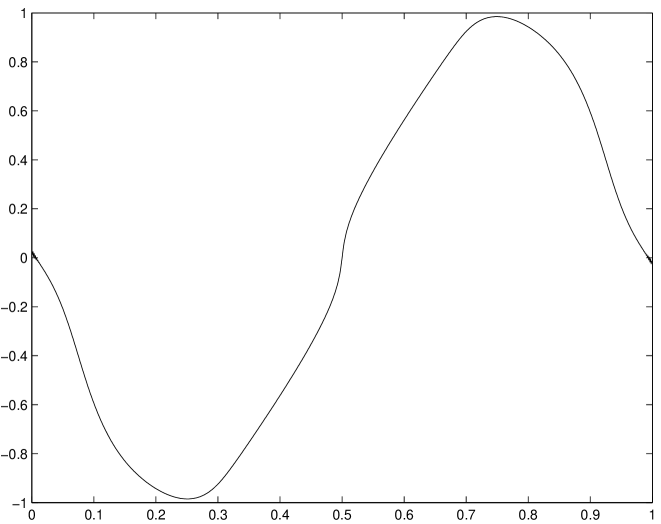
Fig. 2: The graph of $\partial_{x}\phi_{2}(t,x)$ at $t=0.24$.

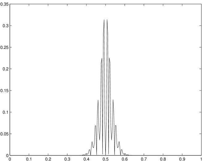
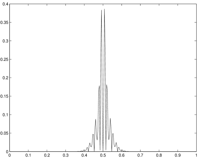
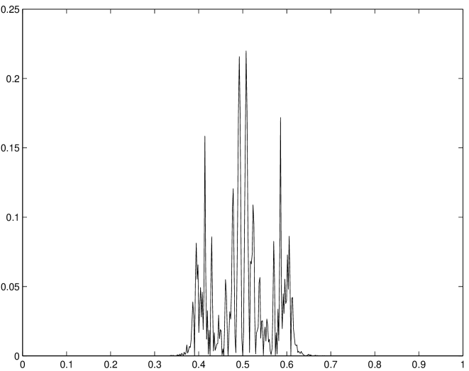
$|\psi^{\rm sc}(x,0.1)|^{2}$, $|\psi^{\rm sc}(x,0.25)|^{2}$, and $|\psi^{\rm sc}(x,0.5)|^{2}$, ${\varepsilon}=\frac{1}{32}$.

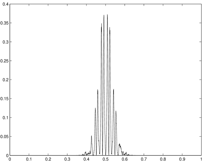
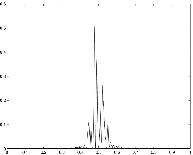
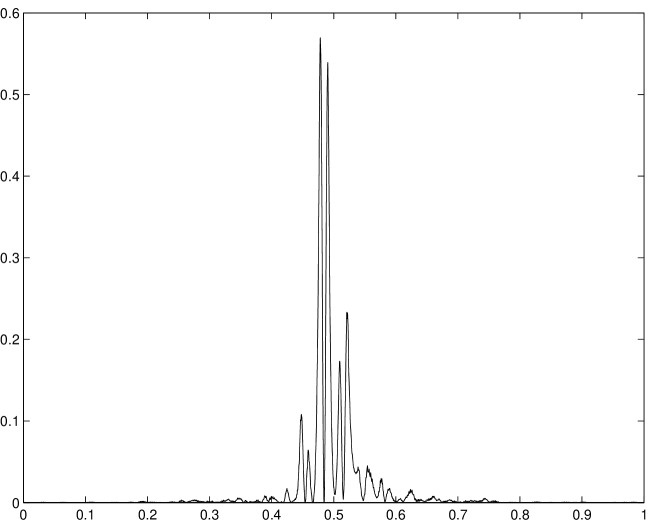
$|\psi^{\rm bd}(x,0.1)|^{2}$, $|\psi^{\rm bd}(x,0.25)|^{2}$, and $|\psi^{\rm bd}(x,0.5)|^{2}$, ${\varepsilon}=\frac{1}{32}$.

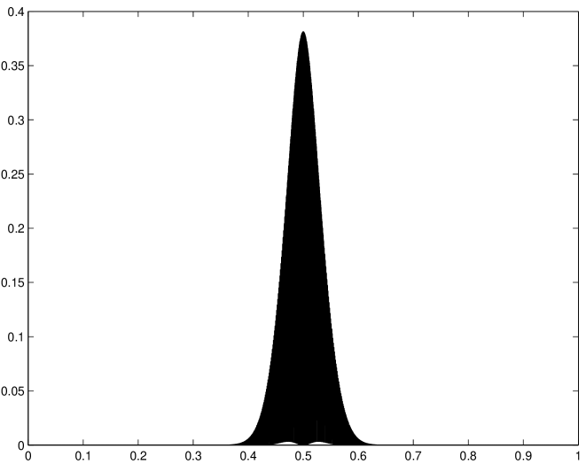
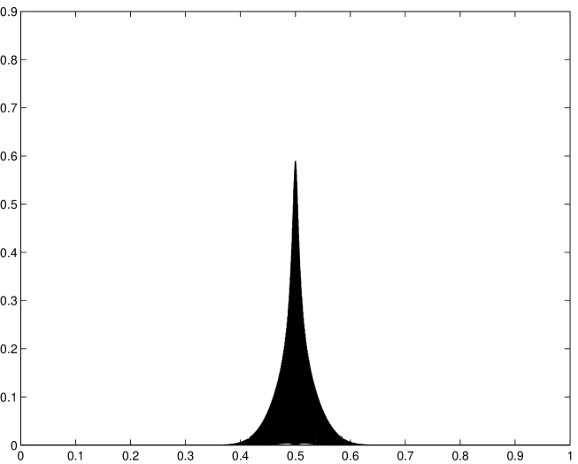
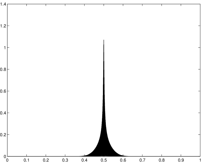
$|\psi^{\rm sc}(x,0.1)|^{2}$, $|\psi^{\rm sc}(x,0.25)|^{2}$, and $|\psi^{\rm sc}(x,0.5)|^{2}$, ${\varepsilon}=\frac{1}{1024}$.

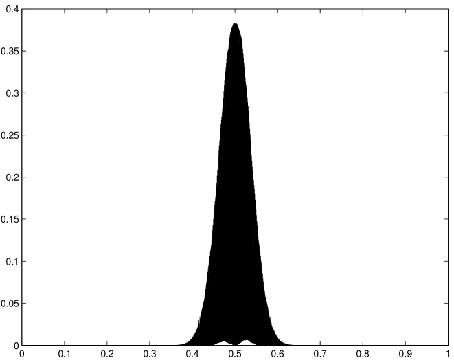
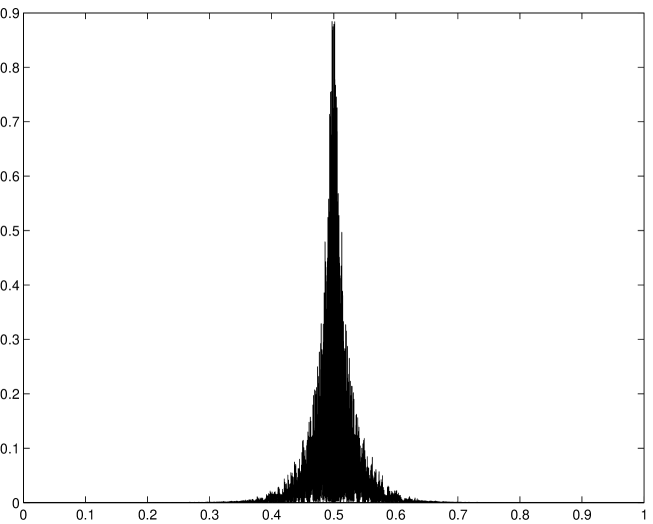
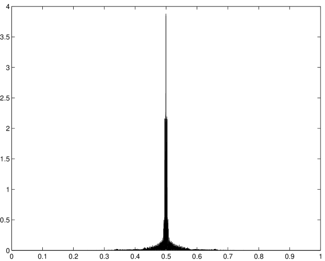
$|\psi^{\rm bd}(x,0.1)|^{2}$, $|\psi^{\rm bd}(x,0.25)|^{2}$, and $|\psi^{\rm bd}(x,0.5)|^{2}$, ${\varepsilon}=\frac{1}{1024}$.

Fig. 15: Numerical results for example 5.2 with $U(x)$ given by (4.3), $\triangle t=\frac{1}{10000}$, $\triangle x=\frac{1}{32768}$. The left column shows the situation before the caustic, whereas the other two columns respectively present the numerical results at and after the caustic.

The corresponding numerical results are given in Fig. 15 and Table 8.

Table 8: Difference between the asymptotic solution and the Schrödinger equation for example 5.2 for initial condition (5.13) ($\triangle t=10^{-4}$, $\triangle x=1/32768$):

${\varepsilon}$	$\frac{1}{32}$	$\frac{1}{1024}$
$\begin{array}[]{c}\vspace{-4mm}\hfil\\ \displaystyle\sup_{0\leq t\leq 0.1}\left\|\,\psi(t,x)-\psi^{\rm sc}(t,x)\,\right\|_{L^{2}({\mathbb{R}})}\end{array}$	$1.68\rm{E}-2$	$3.19\rm{E}-3$
$\begin{array}[]{c}\vspace{-4mm}\hfil\\ \displaystyle\sup_{0\leq t\leq 0.1}\left\|\,\psi(t,x)-\psi^{\rm sc}(t,x)\,\right\|_{L^{\infty}({\mathbb{R}})}\end{array}$	$2.73\rm{E}-1$	$7.33\rm{E}-2$

6 Acknowledgement

The authors are grateful to Prof. Christian Ringhofer for fruitful discussions on this work.

$|\psi^{\rm ex}(t,x)|^{2}$, $|\psi^{\rm ex}(t,x)-\psi^{\rm ts}(t,x)|$ and $|\psi^{\rm ex}(t,x)-\psi^{\rm bd}(t,x)|$ at $t=1.0$

Fig. 3: Numerical results for example 4.1 with $U(x)$ given by (4.2) and ${\varepsilon}=\frac{1}{2}$. We use $\triangle t=\frac{1}{100}$, $\triangle x=\frac{1}{64}$ for the TS and the BD method, and $\triangle t=\frac{1}{100000}$, $\triangle x=\frac{1}{8192}$ for the “exact” solution.

$$\Delta^{\rm ts}_{\infty}(t)=5.39\rm{E}-2,\ \Delta^{\rm bd}_{\infty}(t)=5.07\rm{E}-2,\ \Delta^{\rm ts}_{2}(t)=1.56\rm{E}-2,\ \Delta^{\rm bd}_{2}(t)=1.51\rm{E}-2.$$

$$\Delta^{\rm ts}_{\infty}(t)=1.23\rm{E}-1,\ \Delta^{\rm bd}_{\infty}(t)=1.20\rm{E}-1,\ \Delta^{\rm ts}_{2}(t)=2.29\rm{E}-2,\ \Delta^{\rm bd}_{2}(t)=2.31\rm{E}-2.$$

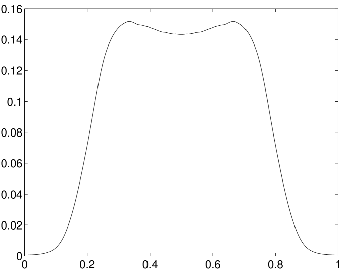
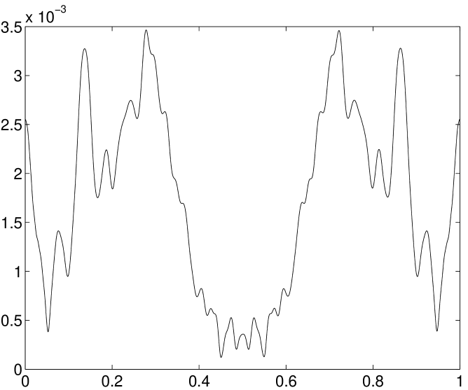
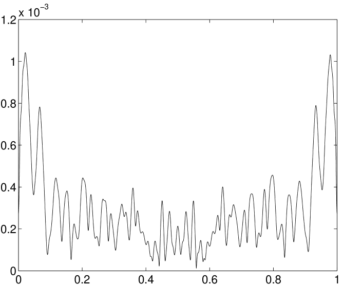
$|\psi^{\rm ex}(t,x)|^{2}$, $|\psi^{\rm ex}(t,x)-\psi^{\rm ts}(t,x)|$ and $|\psi^{\rm ex}(t,x)-\psi^{\rm bd}(t,x)|$ at $t=1.0$

Fig. 5: Numerical results for example 4.1 with $U(x)$ given by (4.3) and ${\varepsilon}=\frac{1}{2}$. We use $\triangle t=\frac{1}{10}$, $\triangle x=\frac{1}{32}$ for the TS and the BD method, and $\triangle t=\frac{1}{100000}$, $\triangle x=\frac{1}{8192}$ for the “exact” solution.

$$\Delta^{\rm ts}_{\infty}(t)=3.47\rm{E}-3,\ \Delta^{\rm bd}_{\infty}(t)=1.04\rm{E}-3,\ \Delta^{\rm ts}_{2}(t)=1.96\rm{E}-3,\ \Delta^{\rm bd}_{2}(t)=3.65\rm{E}-4.$$

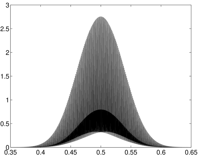
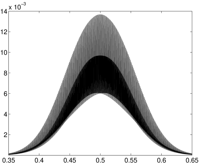
$|\psi^{\rm ex}(t,x)|^{2}$, $|\psi^{\rm ex}(t,x)-\psi^{\rm ts}(t,x)|$ and $|\psi^{\rm ex}(t,x)-\psi^{\rm bd}(t,x)|$ at $t=0.1$

Fig. 6: Numerical results for example 4.1 with $U(x)$ given by (4.3) and ${\varepsilon}=\frac{1}{1024}$. We use Here $\triangle t=\frac{1}{10000}$, $\triangle x=\frac{1}{16384}$ for the TS and $\triangle t=\frac{1}{100}$, $\triangle x=\frac{1}{16384}$ for the BD method, and $\triangle t=\frac{1}{100000}$, $\triangle x=\frac{1}{131072}$ for the “exact” solution.

$$\Delta^{\rm ts}_{\infty}(t)=1.37\rm{E}-2,\ \Delta^{\rm bd}_{\infty}(t)=5.52\rm{E}-3,\ \Delta^{\rm ts}_{2}(t)=2.76\rm{E}-3,\ \Delta^{\rm bd}_{2}(t)=1.20\rm{E}-3.$$

$|\psi^{\rm ex}(t,x)|^{2}$, $|\psi^{\rm ex}(t,x)-\psi^{\rm ts}(t,x)|$ and $|\psi^{\rm ex}(t,x)-\psi^{\rm bd}(t,x)|$ at $t=1.0$

Fig. 7: Numerical results for example 4.1 with $U(x)$ given by (4.4) and ${\varepsilon}=\frac{1}{2}$. We use $\triangle t=\frac{1}{10}$, $\triangle x=\frac{1}{32}$ for the TS and the BD method, and $\triangle t=\frac{1}{100000}$, $\triangle x=\frac{1}{8192}$ for the “exact” solution.

$$\Delta^{\rm ts}_{\infty}(t)=3.26\rm{E}-2,\ \Delta^{\rm bd}_{\infty}(t)=2.72\rm{E}-2,\ \Delta^{\rm ts}_{2}(t)=1.51\rm{E}-2,\ \Delta^{\rm bd}_{2}(t)=1.45\rm{E}-2.$$

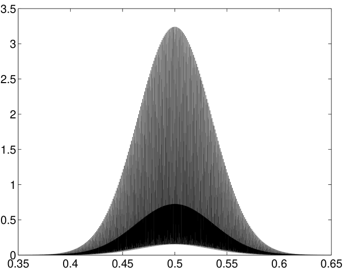
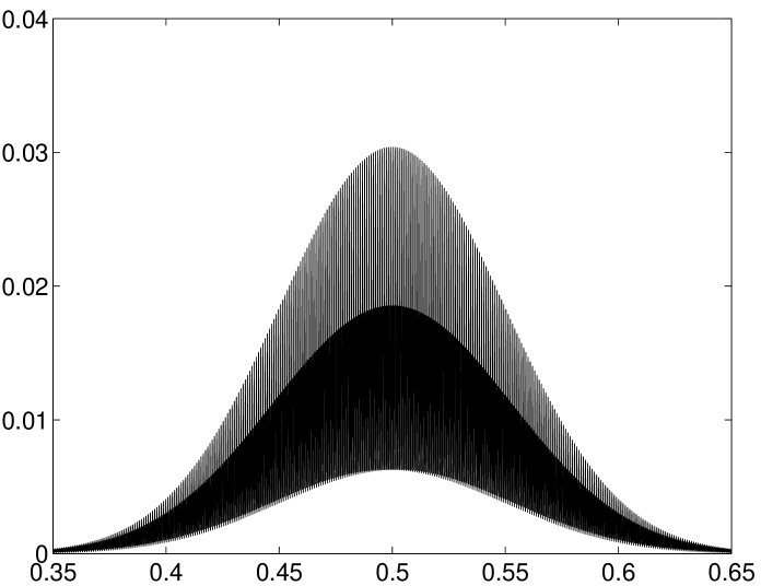
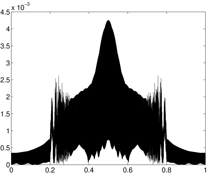
$|\psi^{\rm ex}(t,x)|^{2}$, $|\psi^{\rm ex}(t,x)-\psi^{\rm ts}(t,x)|$ and $|\psi^{\rm ex}(t,x)-\psi^{\rm bd}(t,x)|$ at $t=0.1$

Fig. 8: Numerical results for example 4.1 with $U(x)$ given by (4.4) and ${\varepsilon}=\frac{1}{1024}$. We use $\triangle t=\frac{1}{10000}$, $\triangle x=\frac{1}{16384}$ for the TS and $\triangle t=\frac{1}{10}$, $\triangle x=\frac{1}{8192}$ for the BD method, and $\triangle t=\frac{1}{100000}$, $\triangle x=\frac{1}{131072}$ for the “exact” solution.

$$\Delta^{\rm ts}_{\infty}(t)=3.04\rm{E}-2,\ \Delta^{\rm bd}_{\infty}(t)=4.25\rm{E}-3,\ \Delta^{\rm ts}_{2}(t)=5.35\rm{E}-3,\ \Delta^{\rm bd}_{2}(t)=1.21\rm{E}-3.$$

$$\Delta^{\rm ts}_{\infty}(t)=1.65,\ \Delta^{\rm bd}_{\infty}(t)=9.14\rm{E}-2,\ \Delta^{\rm ts}_{2}(t)=2.63\rm{E}-1,\ \Delta^{\rm bd}_{2}(t)=1.39\rm{E}-2.$$

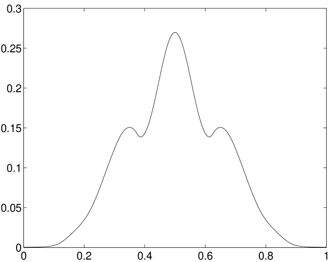
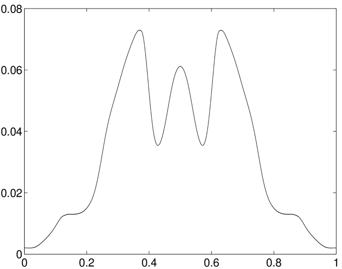
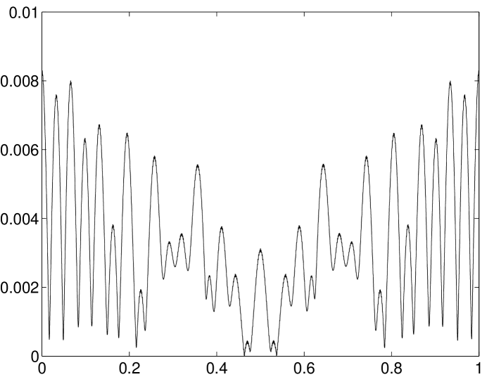
$|\psi^{\rm ex}(t,x)|^{2}$, $|\psi^{\rm ex}(t,x)-\psi^{\rm ts}(t,x)|$ and $|\psi^{\rm ex}(t,x)-\psi^{\rm bd}(t,x)|$ at $t=1.0$

Fig. 11: Numerical results for example 4.2 with $U(x)$ given by (4.3) and ${\varepsilon}=\frac{1}{2}$. We use $\triangle t=\frac{1}{200}$, $\triangle x=\frac{1}{64}$ for the TS, $\triangle t=\frac{1}{5}$, $\triangle x=\frac{1}{32}$ for the BD method, and $\triangle t=\frac{1}{100000}$, $\triangle x=\frac{1}{8192}$ for the “exact” solution.

$$\Delta^{\rm ts}_{\infty}(t)=7.30\rm{E}-2,\ \Delta^{\rm bd}_{\infty}(t)=8.30\rm{E}-3,\ \Delta^{\rm ts}_{2}(t)=4.02\rm{E}-2,\ \Delta^{\rm bd}_{2}(t)=3.89\rm{E}-3.$$

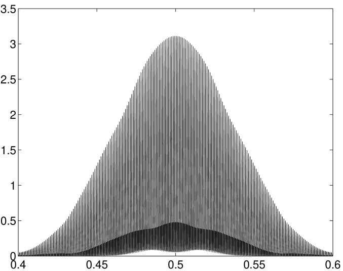
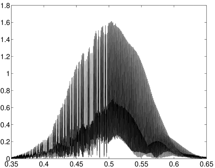
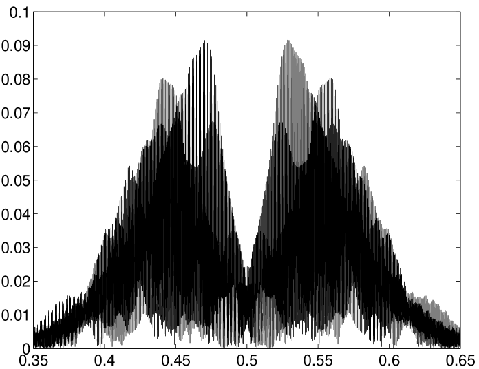
$|\psi^{\rm ex}(t,x)|^{2}$, $|\psi^{\rm ex}(t,x)-\psi^{\rm ts}(t,x)|$ and $|\psi^{\rm ex}(t,x)-\psi^{\rm bd}(t,x)|$ at $t=0.1$

Fig. 12: Numerical results for example 4.2 with $U(x)$ given by (4.3) and ${\varepsilon}=\frac{1}{1024}$. We use $\triangle t=\frac{1}{50000}$, $\triangle x=\frac{1}{65536}$ for the TS, $\triangle t=\frac{1}{10}$, $\triangle x=\frac{1}{8192}$ for the BD method, and $\triangle t=\frac{1}{100000}$, $\triangle x=\frac{1}{131072}$ for the “exact” solution.

$$\Delta^{\rm ts}_{\infty}(t)=1.61,\ \Delta^{\rm bd}_{\infty}(t)=9.16\rm{E}-2,\ \Delta^{\rm ts}_{2}(t)=2.63\rm{E}-1,\ \Delta^{\rm bd}_{2}(t)=1.71\rm{E}-2.$$

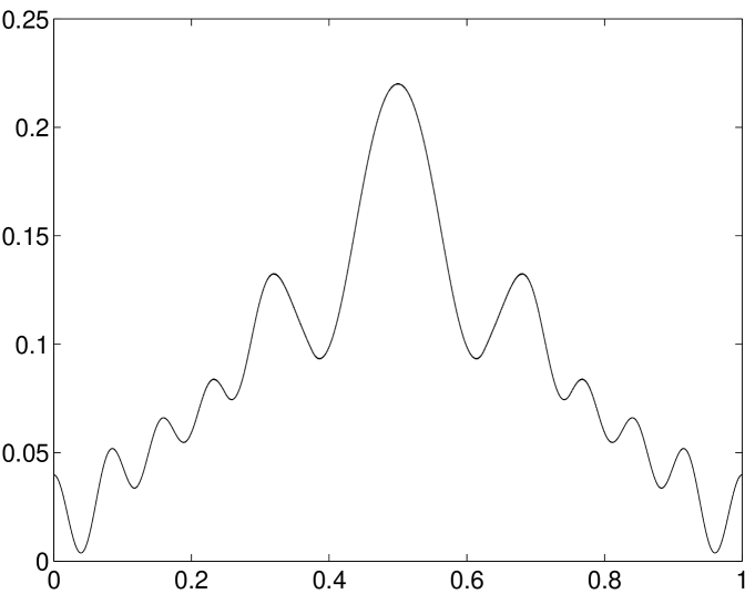
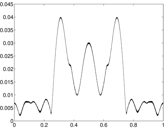
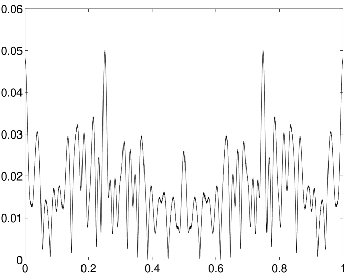
$|\psi^{\rm ex}(t,x)|^{2}$, $|\psi^{\rm ex}(t,x)-\psi^{\rm ts}(t,x)|$ and $|\psi^{\rm ex}(t,x)-\psi^{\rm bd}(t,x)|$ at $t=1.0$

Fig. 13: Numerical results for example 4.2 with $U(x)$ given by (4.4), ${\varepsilon}=\frac{1}{2}$. We use $\triangle t=\frac{1}{100}$, $\triangle x=\frac{1}{32}$ for the TS, $\triangle t=\frac{1}{5}$, $\triangle x=\frac{1}{32}$ for the Bloch-decomposition method, and $\triangle t=\frac{1}{100000}$, $\triangle x=\frac{1}{8192}$for the “exact” solution.

$$\Delta^{\rm ts}_{\infty}(t)=4.01\rm{E}-2,\ \Delta^{\rm bd}_{\infty}(t)=5.00\rm{E}-2,\ \Delta^{\rm ts}_{2}(t)=1.85\rm{E}-2,\ \Delta^{\rm bd}_{2}(t)=1.98\rm{E}-2.$$

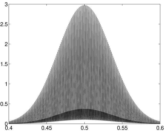
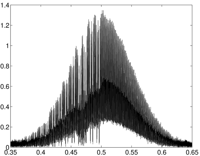
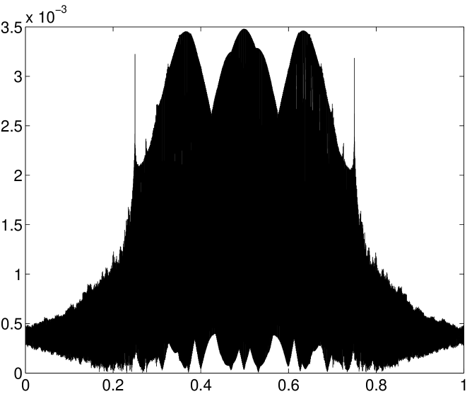
$|\psi^{\rm ex}(t,x)|^{2}$, $|\psi^{\rm ex}(t,x)-\psi^{\rm ts}(t,x)|$ and $|\psi^{\rm ex}(t,x)-\psi^{\rm bd}(t,x)|$ at $t=0.1$

Fig. 14: Numerical results for example 4.2. Here $U(x)$ is given in (4.4), ${\varepsilon}=\frac{1}{1024}$. We use $\triangle t=\frac{1}{10000}$, $\triangle x=\frac{1}{65536}$ for Time-splitting, $\triangle t=\frac{1}{10}$, $\triangle x=\frac{1}{8192}$ for Bloch-decomposition, and $\triangle t=\frac{1}{100000}$, $\triangle x=\frac{1}{131072}$ for ’exact’ solution.

$$\Delta^{\rm ts}_{\infty}(t)=1.35,\ \Delta^{\rm bd}_{\infty}(t)=3.48\rm{E}-3,\ \Delta^{\rm ts}_{2}(t)=2.23\rm{E}-1,\ \Delta^{\rm bd}_{2}(t)=1.14\rm{E}-3.$$

References

- [1] J. Asch and A. Knauf, Motion in periodic potentials, Nonlinearity 11 (1998), 175–200.
- [2] N. W. Ashcroft and N. D. Mermin, Solid state physics, Saunders New York, 1976.
- [3] W. Z. Bao, S. Jin, and P. Markowich, On time-splitting spectral approximations for the Schrödinger equation in the semiclassical regime, J. Comp. Phys. 175 (2002), 487–524.
- [4] W. Z. Bao, S. Jin, and P. Markowich, Numerical study of time-splitting spectral discretizations of nonlinear Schrödinger equations in the semi-Classical regime, SIAM J. Sci. Comp. 25 (2003), 27–64.
- [5] P. Bechouche, N. Mauser, and F. Poupaud, Semiclassical limit for the Schrödinger-Poisson equation in a crystal, Comm. Pure Appl. Math. 54 (2001), no. 7, 851–890.
- [6] P. Bechouche,and F. Poupaud, Semi-classical limit of a Schrödinger equation for a stratified material, Monatsh. Math. 129 (2000), no. 4, 281–301.
- [7] A. Bensoussan, J. L. Lions, and G. Papanicolaou, Asymptotic Analysis for Periodic Structures, North-Holland Pub. Co. (1978).
- [8] F. Bloch, Über die Quantenmechanik der Elektronen in Kristallgittern, Z. Phys. 52 (1928), 555–600.
- [9] E. I. Blount, Formalisms of band theory, Solid State Physics 13, Academic Press, New York, 305–373 (1962).
- [10] K. Busch, Photonic band structure theory: assessment and perspectives, Compte Rendus Physique 3 (2002), 53–66.
- [11] R. Carles, WKB analysis for nonlinear Schrödinger equations with a potential, Comm. Math. Phys. to appear.
- [12] R. Carles, P. A. Markowich and C. Sparber, Semiclassical asymptotics for weakly nonlinear Bloch waves, J. Stat. Phys. 117 (2004), 369–401.
- [13] C. Conca, R. Orive, and M. Vanninathan, Bloch approximation in homogenization on bounded domains, Asymptot. Anal. 41 (2005), no. 1, 71–91.
- [14] C. Conca, N. Srinivasan and M. Vanninathan, Numerical solution of elliptic partial differential equations by Bloch waves method, in: Congress on Differential Equations and Applications/VII CMA (Salamanca, 2001), 63–83, 2001.
- [15] C. Conca and M. Vanninathan, Homogenization of periodic structures via Bloch decomposition, SIAM J. Appl. Math. 57 (1997), no. 6, 1639–1659.
- [16] M. V. Fischetti and S. E. Laux, Monte Carlo analysis of electron transport in small semiconductor devices including band-structure and space-charge effects, Phys. Rev. B 38 (1998), 9721–9745.
- [17] P. Gérard, P. Markowich, N. Mauser, and F. Poupaud, Homogenization Limits and Wigner transforms, Comm. Pure and Appl. Math 50 (1997), 323–378.
- [18] L. Gosse, Multiphase semiclassical approximation of an electron in a one-dimensional crystalline lattice. II. Impurities, confinement and Bloch oscillations, J. Comput. Phys. 201 (2004), no. 1, 344–375.
- [19] L. Gosse and P. A. Markowich, Multiphase semiclassical approximation of an electron in a one-dimensional crystalline lattice - I. Homogeneous problems, J. Comput Phys. 197 (2004), 387–417.
- [20] L. Gosse and N. Mauser, Multiphase semiclassical approximation of an electron in a one-dimensional crystalline lattice. III. From ab initio models to WKB for Schrödinger-Poisson, to appear in J. Comput. Phys. 211 (2006), no. 1, 326–346.
- [21] J. C. Guillot, J. Ralston, and E. Trubowitz, Semiclassical asymptotics in solid-state physics, Comm. Math. Phys. 116 (1998), 401–415.
- [22] D. Hermann, M. Frank, K. Busch, and P. Wölfle, Photonic band structure computations, Optics Express 8 (2001), 167–173.
- [23] R. Horn and C. Johnson, Matrix analysis, Cambridge University Press, Cambridge, 1985.
- [24] Z. Huang, S. Jin, P. Markowich, C. Sparber and C. Zheng, A Time-splitting spectral scheme for the Maxwell-Dirac system, J. Comput. Phys. 208 (2005), issue 2, 761–789.
- [25] S. Jin, Z. Xin, Numerical passage from systems of conservation laws to Hamilton-Jacobi equations, and a relaxation scheme, SIAM J. Num. Anal. 35 (1998), 2385–2404.
- [26] J. D. Joannopoulos and M. L. Cohen, Theory of Short Range Order and Disorder in Tetrahedrally Bonded Semiconductors, Solid State Physics 31 (1974), 1545.
- [27] H. J. Korsch and M. Glück, Computing quantum eigenvalues made easy, Eur. J. Phys. 23 (2002), 413–425.
- [28] S. E. Laux, M. V. Fischetti, and D. J. Frank, Monte Carlo analysis of semiconductor devices: the DAMOCLES program, IBM Journal of Research and Development 34 (1990), 466–494.
- [29] J.M. Luttinger, The effect of a magnetic field on electrons in a periodic potential, Phys. Rev. 84 (1951), 814–817 .
- [30] G. Panati, H. Spohn, and S. Teufel, Effective dynamics for Bloch electrons: Peierls substitution and beyond, Comm. Math. Phys. 242 (2003), 547–578.
- [31] M. Reed, B. Simon, Methods of modern mathematical physics IV. Analysis of operators, Academic Press (1978).
- [32] S. Teufel, Adiabatic perturbation theory in quantum dynamics, Lecture Notes in Mathematics 1821, Springer (2003).
- [33] C. H. Wilcox, Theory of bloch waves, J. Anal. Math. 33 (1978), 146–167.
- [34] J. Zak, Dynamics of electrons in solids in external fields, Phys. Rev. 168 (1968), 686–695.
- [35] A. Zettel, Spectral theory and computational methods for Sturm-Liouville problems, in D. Hinton and P. W, Schäfer (eds.). Lecture Notes in Pure and Applied Math. 191, Dekker 1997.
, and at
, and at
, and at
, and at
, and at
, and at
, and at
, and at
, and at
, and at
, and at
, and at
, , and , .
, , and , .
, , and , .
, , and , .