Origins of Binary Gene Expression in Post-Transcriptional Regulation by MicroRNAs
Abstract
MicroRNA-mediated regulation of gene expression is characterised by some distinctive features that set it apart from unregulated and transcription factor-regulated gene expression. Recently, a mathematical model has been proposed to describe the dynamics of post-transcriptional regulation by microRNAs. The model explains the observations made in single cell experiments quite well. In this paper, we introduce some additional features into the model and consider two specific cases. In the first case, a non-cooperative positive feedback loop is included in the transcriptional regulation of the target gene expression. In the second case, a stochastic version of the original model is considered in which there are random transitions between the inactive and active expression states of the gene. In the first case we show that bistability is possible in a parameter regime, due to the presence of a non-linear protein decay term in the gene expression dynamics. In the second case, we derive the conditions for obtaining stochastic binary gene expression. We find that this type of gene expression is more favourable in the case of regulation by microRNAs as compared to the case of unregulated gene expression. The theoretical predictions relating to binary gene expression are experimentally testable.
1 Introduction
MicroRNAs (miRNAs) are a class of small, noncoding RNAs which regulate gene expression in prokaryotes and eukaryotes at the post-transcriptional level. They play critical roles in a number of cellular processes, such as stress response, developmental transitions, differentiation, apoptosis etc. [1, 2, 3]. The mechanisms of regulation by small RNAs differ in specific features in prokaryotes and eukaryotes. These are, however, based on the common principle of the regulatory RNA base-pairing with the messenger RNA (mRNA) of the target gene inhibiting translation and/or promoting mRNA degradation. Various possibilities have been suggested for the fate of the inactive complex of the regulatory RNA and the target mRNA once it is formed [4, 5, 6, 7]: (i) the complex has a finite lifetime followed by dissociation into its free components, (ii) the regulatory RNA co-degrades with the target mRNA at the same or different rates and (iii) only the target mRNA degrades with the regulatory RNA becoming free for further activity [4, 5, 6, 7]. A number of functional features of RNA-regulated gene expression have been identified so far [4, 6, 7]. One prominent feature is that of a threshold linear mode of action, in which the target gene protein synthesis is highly repressed below a threshold level of target mRNA production and activated in a linear fashion once the threshold is crossed. Other significant characteristics include: suppression of protein fluctuations in the form of translational bursts, rapid response times and filtering of transient signals [7], sharpening of spatial expression patterns [8] and prioritisation of the expression of target genes in the case of a single RNA regulating the expression of multiple genes [9].
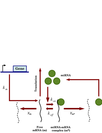
Recently, a mathematical model has been proposed [4] to describe the biochemical interactions and kinetics of miRNA-mediated regulation of gene expression. The model has been experimentally validated in single cell measurements using quantitative fluorescence microscopy and flow cytometry. The experiments clearly demonstrate the high repression of target protein synthesis below a threshold level of target mRNA production, and a sensitive response above the threshold. A major finding is that the strength of the repression below the threshold has considerable cell-to-cell variation in a population of genetically-identical cells. This indicates that stochasticity may have non-trivial consequences in miRNA-mediated regulation of gene expression. Figure 1 shows a sketch of the different biochemical processes involved in the miRNA-mediated regulation of gene expression, and which form the basis of the mathematical model proposed in [4]. The mRNA, as shown in Fig. 1, is either free () or is part of a miRNA-mRNA complex (). The target mRNA is transcribed with rate constant and has a natural degradation rate constant . The rate constants and are associated with the formation and dissociation of the bound complex of mRNA and miRNA. The bound miRNA becomes free either by unbinding the target mRNA (rate constant or by degrading the mRNA (rate constant ). The model incorporates the important feature of molecular titration similar to the protein-protein titration analysed earlier [10]. Protein sequestration occurs when a repressor protein binds an active protein thus forming an inactive complex. As shown in [10], the regulatory mechanism, termed molecular titration, can generate ultrasensitive input-output responses. In the case of miRNA-mediated regulation of gene expression, the inactive complex is that of mRNA and miRNA. Molecular titration is responsible for the observed sensitive dependence of protein expression on target mRNA input around a threshold level of target mRNA production.
In this paper, we analyse the dynamics of the model, the key biochemical processes of which are shown in Fig. 1, from two different perspectives. In the first case, an additional process representing the autoactivation of the target gene expression by the target protein is included. In the second case, a simple stochastic version of the model of Fig. 1 is considered. In this model, the only stochasticity is associated with the random transitions between the inactive and active expression states of the gene. In the inactive state, there is no transcriptional activity, i.e., mRNA synthesis. Transcription is only initiated in the active state of the gene. The degradation of the mRNA occurs in both the inactive and active states of the gene. We show that binary gene expression is a possible outcome in both of the scenarios described above. In the deterministic case, binary gene expression implies bistability, i.e., the coexistence of two stable expression states. In the stochastic case, the distribution of mRNA levels is bimodal, i.e., has two prominent peaks. In the following, we analyse the deterministic and stochastic models to investigate the origins of binary gene expression.
2 Deterministic Model
The total concentration of miRNA is assumed to be constant, since the miRNA turnover is slow compared to the timescale of gene expression [4]. The following set of differential equations describe the dynamics of the model.
| (1) |
| (2) |
| (3) |
The conservation condition for miRNA is
| (4) |
In the equations above, and represent the free and total miRNA concentrations. The second term on the r.h.s. of Eq. (1) represents the autoactivation of the target gene expression. The rate constant represents the maximum rate of mRNA synthesis due to autoactivation, with denoting the equilibrium dissociation constant for the binding of the regulatory protein at the promoter region of the target gene. The rate constants and correspond to protein synthesis and degradation, respectively, with being the protein concentration. In the steady state, , and and one obtains the equations
| (5) |
| (6) |
| (7) |
From these equations, the steady state protein concentration satisfies the equation
| (8) |
with , , , and .
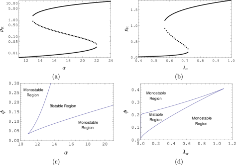
Eq. (8) has two stable steady state solutions, i.e., bistability in specific parameter regions. Figure 2(a) shows a plot of the steady state protein concentration, , as a function of the parameter . The stable steady states are represented by solid lines whereas the dotted line describes the branch of unstable steady states. The plot exhibits hysteresis since the discontinuous transitions from the lower to the upper branch, and from the upper to the lower branch, occur at different values of the parameter , the so-called bifurcation points of the associated dynamics. Bistability constitutes a universal theme in several cell biological processes [11, 12] and signifies that a cell has a choice between two stable expression states for the same parameter values. The choice of the specific stable state depends on the previous history of the system. Figure 2(b) exhibits a plot of versus the parameter . Figure 2(c) shows a phase diagram in the plane in which a region of bistability separates two regions of monostability, corresponding to low and high expression states, respectively. Figure 2(d) shows a similar phase diagram in the plane. Bistability, in general, is an outcome of dynamics involving positive feedback and sufficient nonlinearity. The latter condition is usually achieved via the binding of the regulatory protein molecules at multiple sites of the promoter region of the gene, or when the regulatory proteins form multimers, such as dimers and tetramers, which then bind specific regions of the DNA (cooperativity in regulation) [13, 14]. In the case of transcriptional regulation, Tan et al. [15] have proposed a new mechanism by which a noncooperative positive feedback loop combined with a nonlinear protein decay term are sufficient to generate bistability. This novel type of bistability was demonstrated in the operation of a synthetic gene circuit. The circuit contains a single autoregulatory positive feedback loop in which the protein product X of a gene promotes its own synthesis in a noncooperative fashion. The protein decay rate is a sum of two terms, the natural degradation rate and the dilution rate due to cell growth. In the synthetic circuit, the production of X inhibits cell growth so that the dilution rate of X and hence the protein decay rate are reduced. This gives rise to an effective positive feedback loop, since an increased synthesis of X proteins leads to a greater accumulation of the proteins, which in turn activates further protein synthesis. The combination of two positive feedback loops gives rise to bistability in a parameter regime in the absence of cooperativity. A related study by Klumpp et al. [16] has also demonstrated the generation of a positive feedback loop due to cell growth inhibition by a protein. The nonlinear protein decay term in these cases (‘emergent bistability’) has the same form as in Eq. (8). The origin of the nonlinearity is, however, different in the case of the post-transcriptional, i.e., miRNA-mediated regulation of gene expression. The effect of a transcriptional positive feedback loop on miRNA-regulated gene expression has been investigated in a number of earlier studies [17]. Specifically, bistability has been demonstrated in cases where the transcriptional positive feedback loop involves some form of cooperativity. Our present study establishes a new origin of bistability in miRNA-regulated gene expression, based on a non-cooperative transcriptional positive feedback loop and a nonlinear protein decay term. Since our model closely follows the experimentally-tested model proposed in Ref. [4], the inclusion of a transcriptional positive feedback loop in the original gene circuit could provide an experimental test of the new mechanism of bistability suggested by us.
3 Stochastic Model
The model is a generalisation, incorporating miRNA-mediated regulation of gene expression, of an earlier stochastic model [18] in which the effect of stochasticity on unregulated/transcriptional factor-regulated gene expression was considered. More specifically, the condition for obtaining stochastic binary gene expression in terms of two gene expression parameters, and was derived in the previous study. The rate constants and are the activation and deactivation rate constants for transitions between the inactive and active states of the gene. The rate constant is the degradation rate constant of the gene expression product, which could be either mRNA or protein. In the present study, we determine the steady state distribution of mRNA levels. We assume that the concentration of the mRNA-miRNA complex attains its steady state value at an earlier time point than the concentration of free mRNA. As already mentioned, the only stochasticity in the model considered here is associated with the random transitions between the inactive and active states of the gene. In each state of the gene, the mRNA concentration evolves according to the equation,

| (9) |
Eq. (9) is obtained from Eq. (1) by ignoring the positive feedback term and substituting the steady state concentration of (Eq. (6)). The variable when the gene is in the active (inactive) state and switches values with stochastic rate constants () and () . Let be the probability density function when with the total probability density function . The rate equations for the probability density functions are given by
| (10) |
| (11) |
The first terms in Eqs. (10) and (11) are the so-called ‘transport’ terms, representing the net flow of the probability density. The second terms represent the gain/loss in the probability density due to random transitions between the state () and the other accessible state. In the steady state, both and are zero and the total probability density function satisfies the equation
| (12) |
where
| (13) |
The steady state solution for is given by
| (14) |
where N is the normalisation constant,
| (15) |
and
| (16) |
Putting and i.e., considering only unregulated gene expression, one recovers from Eq. (14) the beta distribution [18, 19]:
| (17) |
where is the normalisation constant. In this case, binary gene expression is obtained in the parameter regime and both . Two prominent peaks in the probability density function appear when and are comparable in magnitude. In the case of transcription-factor regulated gene expression, the effective activation and deactivation rate constants, and , are functions of the regulatory protein (transcription factor) concentration . The gene expression response to a regulatory stimulus may be either graded or binary. The response is quantified in terms of the concentrations of mRNAs/proteins. In graded response, the average steady state concentration of the gene expression product varies continuously as the concentration of the regulatory molecules is changed, until a saturation level is reached. In the case of binary response, gene expression occurs at either of two average levels (say, low or high) and expression at other levels is minimal. The fraction of cells in the low/high expression level changes as is changed. This gives rise to a bimodal distribution in the protein/mRNA levels in an ensemble of cells. In the case of transcription-factor regulated gene expression, binary gene expression is obtained when and . One should point out that in the parameter regime in which binary gene expression occurs, unimodal distributions are obtained when or . The full parameter regime is associated with the system exhibiting binary response to changing activation and deactivation rate constants. For example, for , the probability distribution of mRNA levels has a single peak at a low level. As increases, a second peak appears at a high expression level with the peak becoming more prominent as approaches . At the other extreme of parameter values, , a single peak at the high expression level is obtained. As changes, the position of the peak remains the same, a characteristic of binary response. Stochastic binary gene expression refers to a bimodal distribution of mRNA/protein levels and the bifurcation from a unimodal to a bimodal distribution occurs in the parameter regime and .
In the case of miRNA-mediated regulation of gene expression, the most prominent contribution to binary gene expression is obtained when both and are in Eq. (14), i.e., when the following inequalities are satisfied:
| (18) | |||||
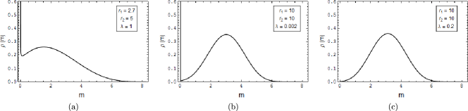
with . One notes that the parameter region in which stochastic binary gene expression may be obtained is expanded from that and in the case of unregulated gene expression. Figure 3 shows the steady state mRNA distribution versus when is and for the parameter values (a) , and (b) , . The other parameter values are and . For each case, the values of are , and respectively. We observe that increasing (decreasing) values of disfavours (favours) bimodality. For , , i.e., the case of unregulated gene expression, binary gene expression occurs in the parameter regime , but not in the regime , . Figure 3 demonstrates the enhanced possibility of binary gene expression in the case of miRNA-mediated regulation of gene expression. One notes that if the parameter is set to zero in Eq. (16), the parameter regime in which binary gene expression is observed is expanded to include all values of the ratio and . The parameter () is analogous to the dissociation constant for the formation of the bound mRNA-miRNA complex with signifying infinitely strong binding. We now provide a physical understanding of the enhanced occurrence of binary gene expression when a miRNA-regulated gene expression parameter, say , is changed.
As mentioned in the Introduction, molecular titration can generate ultrasensitive input-output responses. The origin of ultrasensitivity lies in the sequestration of an active component in an inactive complex through binding to an antagonist [4, 10, 30]. The simple mechanism involves the kinetic scheme

| (19) |
where X represents the active molecule, Y its antagonist and XY the inactive complex. Let be the dissociation constant associated with the complex XY. The total concentrations of X and Y are given by and . When , the X versus plot exhibits ultrasensitivity with the threshold set by . For , almost all the X molecules are part of the inactive complex so that the concentration of free X molecules is very low. At the threshold point , the sequestration of X molecules is no longer dominant, so that a small increase in can give rise to a large increase in X. The sharpness of the ultrasensitive response in the simple example is controlled by the ratio [10]. In the present study, X and Y represent the mRNA and the miRNA respectively. When is in Eq. (14), a dominant singularity occurs at the point , with the expression for given in Eq. (16). In terms of the original parameters, is given by
| (20) |
where , and is given by the expression in Eq. (6). The magnitude of is a measure of the total amount of mRNA. When the effective dissociation constant , we obtain
| (21) | |||||
| (22) | |||||
| (23) |
The constant is proportional to the total amount, , of miRNAs and sets the threshold of an ultrasensitive steady state response. Figure 4 (a) shows the steady state versus plots (Eq. (20)) on a semi-logarithmic scale for the values of (dash-dotted line), (dashed line), (thin solid line) and (thick solid line). One finds that the ultrasensitive behaviour is prominent only when is close to zero. The value of is fixed at the value 2. Figures 4 (b)-(d) show the steady state versus curves (Eq. (14)) for the parameters values , and greater than (b), almost equal to (c) and less than (d). In the last case, the second peak at ( in Eq. (14)) occurs very close to the peak at ().
The inequalities in Eq. (18) can be rewritten in a simpler form
| (24) |
with and .
The rate constants and can be interpreted as effective mRNA decay rate constants by noting the following. From Eq. (9), for , i.e., when the target gene is in the inactive state,
On linearising around the steady state value , one obtains
| (25) |
Similarly, for , i.e., when the target gene is in the active state, . Again, linearising around the steady state value , one gets
| (26) |
Eqs. (23) and (24) are identical in forms to the equations obtained in the case of unregulated gene expression. In the latter case, however, . The origin of binary gene expression in the parameter regime , now has a clear physical interpretation. In the inactive state of the gene, the activation rate constant has a lower value than that of the effective mRNA degradation rate constant so that the accumulated protein level can decay to the steady state level before the next transition to the active state of the gene occurs. Similarly, in the active state of the gene, the deactivation rate constant has a magnitude lower than that of the effective mRNA degradation rate constant . The gene is thus in the active state for a sufficiently long time so that the steady state mRNA level (Eq. (20)) is attained. The parameter regime (Eq. (22)) corresponds to binary response in gene expression as changing the , values does not alter the peak positions but only the amplitudes. When both and are , the activation/deactivation rate constant is larger than the effective mRNA degradation rate constant, so that a transition from the inactive to the active state and vice versa occurs before the mRNA level can attain the value in the inactive state, and the value in the active state. As a result, the probability distribution is unimodal, with the peak position at an intermediate mRNA level. One also obtains a graded response to changing values of the rate constants and , i.e., the position of the peak shifts in a graded manner. In the steady state expression for , for and , the singularities occur at and . The other terms add a small background correction to the distribution. Figure 5 shows the plot of versus in the case when and , (). In this case, though a bimodal distribution is obtained for , and small, the second peak is associated with quite a broad distribution ((a) and (b)). When the magnitude of is increased from (b) to (c), a unimodal distribution is obtained.
4 Conclusion
Theoretical modeling studies combined with experiments have been spectacularly successful in uncovering novel features of cellular phenomena. One such feature is that of binary gene expression, in which the distribution of mRNA/protein levels has two prominent peaks. The possible origins of binary gene expression are several of which three principal mechanisms have been the focus of recent studies [20]: positive feedback-based [12, 13], emergent bistability [15, 21] and purely stochastic [18, 22, 23, 24, 25, 26, 27]. The first two mechanisms create the potential for the coexistence of two stable expression states and noise-induced transitions between the states give rise to the bimodal nature of the distribution of mRNA/protein levels. In the case of binary gene expression with a purely stochastic origin, there is no bistability in the deterministic limit. Experimental observations of stochastic binary gene expression have been reported in a number of studies [24, 25, 27], in agreement with theoretical results. The large number of studies carried out so far on binary gene expression consider the expression to be unregulated or transcription-factor regulated. The issue of binary gene expression in the case of post-transcriptional regulation of gene expression has been mostly confined to the investigation of models in which both transcriptional and post-transcriptional (e.g., miRNA-regulated) modes of regulation are considered and the transcriptional regulation involves a cooperative positive feedback. In this paper, we have discussed two possible scenarios for miRNA-mediated regulation of gene expression, one deterministic and the other stochastic, and demonstrated the existence of binary gene expression in each case. In the first case, a nonlinear protein decay term, together with a noncooperative positive feedback term generate bistability in specific parameter regimes. In the second case, the conditions for obtaining stochastic binary gene expression are obtained and one finds that the parameter region in which binary gene expression occurs is more extended in comparison with the cases of unregulated and transcription factor-regulated gene expression. In the latter two cases, slow transitions between the inactive and active gene expression states are responsible for binary gene expression. The conditions and can be reexpressed as and with , being the average lifetimes of the active and inactive gene expression states (, ) and is the average lifetime of the mRNAs. In the case of miRNA-mediated regulation of gene expression, ultrasensitivity generated by molecular titration plays a key role in the generation of binary gene expression. The conditions and (Eq. (22)) set new time scales in the characterisation of the ‘slowness’ of the transitions between the gene expression states. This results in an expanded parameter regime in which binary gene expression is observed. The theoretical predictions made in the present study could be tested in experiments involving natural and synthetic gene circuits.
Binary gene expression generates phenotypic heterogeneity in a cell population with identical genetic makeup and exposed to the same initial conditions and environment. Microorganisms adopt a number of strategies for coping with stressful situations like environmental fluctuations, nutrient depletion and application of antibiotic drugs. One such strategy is the creation of phenotypic heterogeneity so that the whole population does not suffer the same fate when subjected to stress [28, 29, 30]. Recent experiments on E. coli [28, 29], B. Subtilis [30] and M. Smegmatis [31, 32] have demonstrated the advantages of phenotypic heterogeneity when microorganisms are subjected to stress. The regulation of gene expression by miRNAs is known to be activated in a number of cases in which a cell population is subjected to stress [1, 2, 3]. Experimental evidence of phenotypic heterogeneity in the form of binary gene expression due to regulation by miRNAs would be of significant interest in the context of the response of cell populations to stressful conditions.
Acknowledgment
SG acknowledges the support by CSIR, India, under Grant No. 09/015(0361)/2009-EMR-I.
References
- [1] M. Inui, G. Martello and S. Piccolo, Nat. Rev. Mol. Cell. Biol. 11(4), 252 (2010)
- [2] A. S. Flynt and E. C. Lai, Nat. Rev. Genet. 9, 831 (2008)
- [3] A. K. L. Leung and P. A. Sharp, Mol. Cell 40, 205 (2010)
- [4] S. Mukherji, M. S. Ebert, G. X. Y. Zheng, J. S. Tsang, P. A. Sharp and A. van Oudenaarden, Nat. Genetics 43, 854 (2011)
- [5] Z. L. Whichard, A. E. Motter, P. J. Stein and S. J. Corey, J. Biol. Chem. 286(6), 4742 (2011)
- [6] E. Levine E, Z. Zhang, T. Kuhlman and T. Hwa, PLoS Biol. 5(9): e229 (2007)
- [7] E. Levine and T. Hwa, Curr. Opin. in Microbiol. 11, 574 (2008)
- [8] E. Levine, P. McHale and H. Levine, PLoS Comp. Biol. 3: e233 (2007)
- [9] N. Mitarai, A. M. C. Andersson, S. Krishna, S. Searsey and K. Sneppen, Phys. Biol. 4, 164 (2007)
- [10] N. E. Buchler and M. Louis, J. Mol. Biol. 384, 1106 (2008)
- [11] W. K. Smits, O. P. Kuipers and J. -W. Veening, Nat. Rev. Microbiol. 4, 259 (2006)
- [12] J. R. Pomerening, Curr. Opin. Biotechnol. 19, 381 (2008)
- [13] J. E. Ferrell Jr. , Curr. Opin. Cell Biol. 14, 140 (2002)
- [14] A. Y. Mitrophanov and E. A. Groisman, Bioessays 30, 542 (2008)
- [15] C. Tan, P. Marguet and L. You, Nat. Chem. Biol. 5, 842 (2009)
- [16] S. Klumpp, Z. Zhang and T. Hwa, Cell 139, 1366 (2009)
- [17] V. Zhadnov, Phys. Rep. 500, 1 (2011)
- [18] R. Karmakar and I. Bose, Phys. Biol. 1(3-4), 197 (2004)
- [19] A. Raj, C. S. Peskin, D. Tranchina, D. Y. Vargas and S. Tyagi, PLoS Biol 4(10): e309 (2006)
- [20] I. Bose, Science and Culture 78, 113 (2012)
- [21] S. Ghosh, S. Banerjee and I. Bose, Eur. Phys. J. E 35:11, 1 (2012)
- [22] M.S. Ko, J. Theor. Biol. 153, 181 (1991)
- [23] T. B. Kepler and T. C. Elston, Biophys. J. 81, 3116 (2001)
- [24] M. Kærn, T. C. Elston, W. J. Blake, and J. J. Collins, Nature Rev. Genet. 6, 451 (2005)
- [25] A. Raj and A. van Oudenaarden, Cell 135, 216 (2008)
- [26] R Karmakar and I. Bose, Phys. Biol. 4, 29 (2007)
- [27] T. L. To and N. Maheshri, Science 327, 1142 (2010)
- [28] G. Balázsi, A. van Oudenaarden, and J. J. Collins Cell 144, 910 (2011)
- [29] N. Q. Balaban, Curr Opin Genet Dev. 21(6), 768 (2011)
- [30] J. -W. Veening, W. K. Smits and O. P. Kuipers, Annu Rev Microbiol. 62, 193 (2008)
- [31] K. Sureka, B. Ghosh, A. Dasgupta, J. Basu, M. Kundu and I. Bose, PLoS ONE 3(3): e1771 (2008)
- [32] S. Ghosh, K. Sureka, B. Ghosh, I. Bose, J. Basu and M. Kundu, BMC Syst. Biol. 5, 18 (2011)