Quantum Magnetism of Spin-Ladder Compounds with Trapped-Ion Crystals

Abstract

The quest for experimental platforms that allow for the exploration, and even control, of the interplay of low dimensionality and frustration is a fundamental challenge in several fields of quantum many-body physics, such as quantum magnetism. Here, we propose the use of cold crystals of trapped ions to study a variety of frustrated quantum spin ladders. By optimizing the trap geometry, we show how to tailor the low dimensionality of the models by changing the number of legs of the ladders. Combined with a method for selectively hiding of ions provided by laser addressing, it becomes possible to synthesize stripes of both triangular and Kagome lattices. Besides, the degree of frustration of the phonon-mediated spin interactions can be controlled by shaping the trap frequencies. We support our theoretical considerations by initial experiments with planar ion crystals, where a high and tunable anisotropy of the radial trap frequencies is demonstrated. We take into account an extensive list of possible error sources under typical experimental conditions, and describe explicit regimes that guarantee the validity of our scheme.

I Introduction

The transition from single-particle to many-body quantum systems yields one of the most interesting concepts of physics: emergence. As emphasized by P. W. Anderson emergence , the laws that describe the collective behavior of interacting many-body systems can be fundamentally different from those that govern each of the individual particles. This effect leads to some of the most exotic phenomena of condensed-matter physics in the last decades wen_book . Unfortunately, the high complexity of many-body systems turns our endeavor to understand such emergent phenomena into a fundamental challenge for both experimental and theoretical physics. Since exact analytical solutions seldom exist, even for oversimplified models, one is urged to develop efficient numerical methods. An alternative to this approach are the so-called quantum simulations qs , which make use of a particular quantum system that can be experimentally controlled to a high extent, in order to unveil the properties of a complicated interacting many-body model.

There are two different strategies for the quantum simulation of many-body systems qs_review , the so-called analog and digital quantum simulators (QSs). On the one hand, an ideal analog QS would be a dedicated experimental device where one can prepare the quantum state, engineer a Hamiltonian of interest, and measure its properties. On the other hand, a digital QS aims at reproducing the dynamics of any given Hamiltonian by concatenating a set of available quantum gates. Independently of their particular experimental implementation, these types of QSs would be capable of exploring models from very different areas of physics, ranging from condensed-matter to high-energy physics. Let us remark that this enterprise benefits directly from the development of architectures for quantum-information processing qs_insight . In this work, we focus on one of these architectures: laser-cooled atomic ions confined in radio-frequency traps ion_trap_reviews . Here, some remarkable quantum simulations have already been accomplished in experiments, either in the digital digital_qs or analog ising_ions ; frustration_monroe ; ising_monroe ; dirac_gerritsma ; ising_bollinger versions. In particular, we shall concentrate on analog QSs, where a number of theoretical proposals already exist ion_qsimulator_reviews . Some of these proposals target the quantum simulation of relativistic effects relativistic_effects , quantum spin models ising_porras ; spin_models_ti ; frustration_duan ; frustration_ulm , many-body boson systems bosons_ti , spin-boson models spin_boson_ti , or theories of quantum transport and friction frenkel_kontorova .

A direction of research that is being actively explored is the QS of magnetism ising_porras , which yields a playground for a variety of cooperative quantum many-body effects. Even though the phenomenon of magnetic ordering was already known to the ancient greeks, the understanding of its microscopic origin could only be achieved after the development of quantum mechanics. A particular topic of recurring interest is the fate of the magnetically-ordered phases in the presence of quantum fluctuations lechemitant_book , which get more pronounced as the dimensionality of the system is reduced. Such quantum fluctuations may destroy the long-range order, favoring paramagnetic phases and triggering the so-called quantum phase transitions sachdev_book . Alternatively, they may stabilize more interesting phases, such as the long-sought two-dimensional quantum spin liquids, which have connections with the theory of high-temperature superconductivity rvb_anderson . The advent of a QS for quantum magnetism would allow for an unprecedented experimental realization of these phases, addressing puzzles that remain unsolved due to their great complexity.

A representative model that exemplifies the usefulness of analog QS is the one-dimensional quantum Ising model tfi , which describes a chain of interacting spins subjected to a transverse magnetic field. This model has traditionally been considered as a cornerstone in the theory of quantum phase transitions sachdev_book . However, the vast majority of low-dimensional materials realize instances of the so-called Heisenberg model (see e.g. heisenberg_materials ). In fact, the demanding requirements to explore the Ising magnetism in real materials (e.g. precise one-dimensionality, strong Ising anisotropy, and weak exchange couplings matching the available magnetic fields) have postponed its observation until the recent experiments with CoNb₂O₆ tfi_solid ; note ; cobalt_balents ; cobalt_moore . We stress that prior to this experiment, trapped-ion QSs had already targeted the onset of Ising criticality ising_ions ; ising_monroe . More recently, Ising interactions in a large collection of ions have been observed in Penning traps ising_bollinger , which in combination with the recent results for neutral atoms tfi_atoms , yield the unique possibility of tailoring the microscopic properties of the quantum Ising magnet (e.g. couplings, dimensionality, geometry).

In this manuscript, we investigate the capabilities of trapped ions as QSs of frustrated quantum Ising models (FQIMs). Here, frustration arises from the impossibility of minimizing simultaneously a set of competing commuting interactions (i.e. classical frustration) ising_af_triangular , whereas the quantum fluctuations are introduced by a transverse magnetic field. We remark that, with the exceptions of three-dimensional spin ice spin_liquid and some disordered spin-glass compounds itf_glass , most of the frustrated materials correspond once more to Heisenberg magnets frustration_materials . This would turn the extensive research on low-dimensional frustrated Ising models frustration_book ; qim_frustration into a pure theoretical enterprise. Fortunately, the seminal experiment frustration_monroe has proved the contrary by demonstrating that the physics of small frustrated networks frustration_duan can be explored in trapped-ion laboratories. In a recent work frustration_ulm , we have studied a different approach to control the degree of frustration in ion crystals, which works independently of the number of ions and is thus amenable of being scaled to large systems. In this manuscript, we elaborate on that proposal to develop a versatile quantum simulator for a variety of spin ladder geometries.

A quantum spin ladder is an array of coupled quantum spin chains. Each of these spin chains is usually known as a leg of the ladder, whereas the couplings between them define the ladder rungs. Let us note that the study of antiferromagnetic Heisenberg ladders has a long tradition inspired by the experiments with insulating cuprate compounds heisenberg_spin_ladders , which become high-temperature superconductors after doping superconductors . These strongly-correlated systems lead to fascinating and thoroughly-studied phenomena ladder_sierra . In contrast, the quantum Ising ladders have remained largely unexplored, probably due to the absence of materials that realize them. Our work discusses a proposal to fill in such gap, which is based on techniques of current trapped-ion experiments.

This article is organized as follows. In Sec. II, we describe the properties of the ladder compounds formed by a collection of ions confined in a radio-frequency trap. We discuss the experimental conditions leading to a particular vibrational band structure, which shall be exploited to explore the physics of magnetic frustration. In section III, we support the above conclusions by the numerical simulation of a particular case: the trapped-ion zigzag ladder. A discussion of the experimental feasibility of our scheme with state-of-the-art setups is also presented in Sec. IV. Here, we also present initial experiments regarding the appropriate trap design for the QS, and discuss possible sources of error. In Sec. V, we list the many-body phenomena that can be addressed with the proposed QS, ranging from ordered phases of quantum dimer models, to disordered quantum spin liquids. In Sec. VI, we address in detail the phase diagram of the dipolar $J_{1}$-$J_{2}$ quantum Ising model. Finally, we present our conclusions in Sec. VII. In the Appendixes A, B and C, we discuss technical details regarding both the spin-dependent dipole forces and spontaneous decay, the micromotion, and the thermal secular motion. We describe conditions under which they do not affect the proposed QS.

II Trapped-Ion Quantum Ising Ladders

II.1 Geometry of the trapped-ion ladders

An ensemble of $N$ atomic ions of mass $m$, and charge $e$, can be trapped in a microscopic region of space by means of radio-frequency fields ion_trap_reviews . This system is described by

$$H=\sum_{i=1}^{N}\sum_{\alpha=x,y,z}\!\!\left(\frac{1}{2m}{p}_{i\alpha}^{2}+\frac{1}{2}m\omega_{\alpha}^{2}r_{i\alpha}^{2}\!\right)\!+\frac{e^{2}}{2}\sum_{i}\sum_{j\neq i}\frac{1}{|{\bf r}_{i}-{\bf r}_{j}|},$$ (1)

where $\{\omega_{\alpha}\}_{\alpha=x,y,z}$ represent the effective trapping frequencies (see also Sec. IV and Appendix B), and $\{{\bf r}_{i},{\bf p}_{i}\}_{i=1}^{N}$ are the positions and momenta of the ions. Note that we use gaussian units and $\hbar=1$ throughout this text.

With the advent of laser cooling, it has become possible to reduce the temperature of the ions to such an extent that they crystallize. This gives rise to one of the forms of condensed matter with the lowest attained density, ranging from clusters composed by two ions coulomb_crystal_exps , to crystals of several thousands other_ion_crystals . Interestingly, these crystals can be assembled sequentially by increasing the number of trapped ions one by one, so that the aforementioned transition to the many-body regime emergence can be studied in the laboratory. Besides, the geometry of the crystals can be controlled experimentally by tuning the anisotropy of the trapping frequencies structural_theory , which opens a vast amount of possibilities for the QS of magnetism.

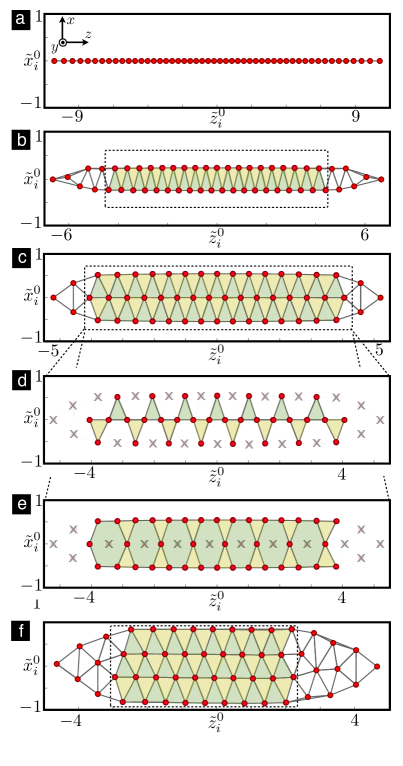
Figure 1: Trapped-ion ladders: Self-assembled geometries for $N$ trapped ions as a function of the anisotropic trapping frequencies $\omega_{y}\gg\omega_{x},\omega_{z}$: (a) Linear chain for $N=50$ and $\kappa_{x}=4\cdot 10^{-4}$, (b) Two-leg zigzag ladder for $N=51$ and $\kappa_{x}=1\cdot 10^{-2}$. (c) Three-leg ladder of bond-sharing triangles for $N=52$ and $\kappa_{x}=4\cdot 10^{-2}$, (d) Two-leg ladder of corner-sharing triangles for $N=52$. From this geometry, it is possible to obtain the two following ladders by selectively hiding some of the ions (grey crosses) following the methods outlined in Sec. IV. (e) Three-leg ladder corresponding to a Kagome stripe of corner-sharing triangles and hexagons for $N=52$, (f) Four-leg ladder of corner-sharing triangles for $N=53$ and $\kappa_{x}=8\cdot 10^{-2}$.

The ion equilibrium positions $\{{\bf r}_{i}^{0}\}_{i=1}^{N}$ are determined by the balance of the trapping forces and the Coulomb repulsion. Formally, they are given by $\bm{\nabla}_{{\bf r}_{i}}V={\bf 0}$, where $V$ contains the trapping and Coulomb potentials. By introducing the unit of length $l_{z}=(e^{2}/m\omega_{z}^{2})^{1/3}$, the dimensionless equilibrium positions $\tilde{{\bf r}}_{i}^{0}={\bf r}_{i}^{0}/l_{z}$ follow from the solution of the system

$${\tilde{r}}_{i\alpha}^{0}-\kappa_{\alpha}\sum_{j\neq i}\frac{{\tilde{r}}^{0}_{i\alpha}-{\tilde{r}}^{0}_{j\alpha}}{|{\tilde{\bf r}}^{0}_{i}-{\tilde{\bf r}}^{0}_{j}|^{3}}=0,\hskip 8.61108pti=1\dots N,\hskip 2.15277pt\alpha=x,y,z,$$ (2)

where we have introduced the anisotropy parameters $\kappa_{\alpha}=(\omega_{z}/\omega_{\alpha})^{2}$. As shown in the experiments exps_zig_zag , by increasing the parameters $\kappa_{x}=\kappa_{y}$ towards a maximum value $\kappa_{\rm max}=1$, the geometry of the ion crystal undergoes a series of phase transitions starting from a linear chain, via a two-dimensional zigzag ladder, to a three-dimensional helix. We remark that these structural phase transitions have been the subject of considerable interest on their own zig_zag_theory ; zigzag_inhomogeneous .

We have recently investigated the possibility of setting a large anisotropy between the radial trap frequencies $1\geq\kappa_{x}\gg\kappa_{y}$, such that the ion crystals get pinned to the $xz$-plane frustration_ulm . This requires a modification of the symmetric electrode configuration of the usual linear traps (see the details in Sec. IV). Besides, the parameter $\kappa_{x}$ can be increased by a bias voltage, yielding a variety of geometries. For instance, above a certain value $\kappa_{\rm c,2}$, the linear chain transforms onto a $2$-leg ladder (see Figs. 1(a)-(b)). By solving numerically the system of equations (2), we observe that the 2-leg zigzag ladder first evolves into a 3-leg ladder as $\kappa_{x}$ is increased, then yields a 4-leg ladder [see Figs. 1(c) and 1(f)], and so on. Hence, there should be a sequence of structural transitions at the critical values $\kappa_{\rm c,2}<\kappa_{\rm c,3}<\kappa_{\rm c,4}<\dots<\kappa_{{\rm c},n_{\rm l}}$, where $n_{\rm l}$ determines the number of legs of the trapped-ion ladders. The rungs of these ladders correspond to the diagonal links, yielding a collection of bond-sharing triangular plaquettes. In Sec. IV, we describe a method to build ladders from corner-sharing triangles (see Figs. 1(d)-(e)), which widens the applicability of our QS.

Eventually, when $\kappa_{x}\to 1$, the crystal must correspond to a two-dimensional bond-sharing triangular lattice, or corner-sharing Kagome lattice, with ellipsoidal boundaries. Accordingly, not only can we control the number of legs of the trapped-ion ladder, but also explore the crossover from quasi-one-dimensional physics to the two-dimensional realm. With respect to the FQIMs, this two-dimensional limit is very appealing due to its connection to quantum spin liquids rvb_anderson , and quantum dimer models qim_frustration . However, as happens for Heisenberg magnets heisenberg_spin_ladders , the ladder compounds may already contain fascinating phenomenology. Let us remark that the precise knowledge of the crystal plane is a fundamental advantage for the quantum simulation of FQIM frustration_ulm . Prior to the discussion of the effective FQIM, we will describe the collective vibrational modes in these ladder compounds, since they shall act as mediators of the magnetic Ising-type interaction.

At this point, it is worth commenting on the possibility of engineering the lattice positions of the ion crystal by means of micro-fabricated electrode arrangements, (e.g. surface traps as proposed in surface_traps ). If the technical problems related to the anomalous heating observed close to the electrodes are overcome, these new generation of traps could be combined with the proposed QS to study frustrated spin models in arbitrary lattices without the complication of micromotion. However, to keep within reach of the current technology, we focus on the more standard Paul traps where experiments on quantum magnetism have already been performed ising_ions ; frustration_monroe ; ising_monroe .

II.2 Collective vibrational modes of the ion ladder

Due to the Coulomb interaction, the vibrations of the ions around the equilibrium positions, ${\bf r}_{i}={\bf r}_{i}^{0}+\Delta{\bf r}_{i}$, become coupled. By expanding the Hamiltonian (1) to second order in the displacements $\Delta{\bf r}_{i}$, one obtains a model of coupled harmonic oscillators corresponding to the harmonic approximation

$$H=\!\sum_{i,\alpha}\!\left(\frac{1}{2m}{p}_{i\alpha}^{2}+\frac{1}{2}m{\omega}_{\alpha}^{2}\Delta r_{i\alpha}^{2}\!\right)\!+\!\frac{1}{2}\sum_{i,j,\alpha,\beta}\mathcal{V}_{ij}^{\alpha\beta}\Delta r_{i\alpha}\Delta r_{j\beta}.$$ (3)

In this expression, the coupling matrix between the harmonic oscillators can be expressed in terms of the mutual ion distance ${\bf r}^{0}_{ij}={\bf r}^{0}_{i}-{\bf r}^{0}_{j}$, and the quadrupole moment for each pair of ions $Q^{\alpha\beta}_{ij}=-e[3({\bf r}^{0}_{ij})_{\alpha}({\bf r}^{0}_{ij})_{\beta}-\delta_{\alpha\beta}({\bf r}^{0}_{ij})^{2}]$ as follows

$$\mathcal{V}_{ij}^{\alpha\beta}=\frac{eQ^{\alpha\beta}_{ij}}{|{\bf r}^{0}_{ij}|^{5}}-\left(\sum_{l\neq i}\frac{eQ^{\alpha\beta}_{il}}{|{\bf r}^{0}_{il}|^{5}}\right)\delta_{ij}.$$ (4)

For the particular ladder geometries in Fig. 1, we identify two types of vibrational excitations, the so-called transverse modes that correspond to the vibrations of the ions perpendicular to the ladder (i.e. $y$-axis), and the planar modes that account for the coupled vibrations within the ladder (i.e. $x,z$ axes). The transverse modes are decoupled from the planar vibrations, and are described by a set of coupled oscillators

$$H_{\bot}\!=\!\sum_{i}\left(\frac{1}{2m}{p}_{iy}^{2}+\frac{1}{2}m\tilde{{\omega}}_{iy}^{2}\Delta r_{iy}^{2}\right)+\frac{e^{2}}{2}\sum_{i}\sum_{j\neq i}\frac{1}{|{\bf r}_{ij}^{0}|^{3}}\Delta r_{iy}\Delta r_{jy},$$ (5)

where $\omega_{y}^{2}\to\tilde{{\omega}}_{iy}^{2}={\omega}_{y}^{2}(1-\kappa_{y}\sum_{l\neq i}|{\bf\tilde{r}}_{l}^{0}-{\bf\tilde{r}}_{i}^{0}|^{-3})$. This term amounts to the Einstein model of individual lattice vibrations, where the renormalization of the frequencies is caused by the mean-field-type interaction of one ion with the rest of the ion ensemble. In our case, we must also consider the coupling between distant oscillators, whose magnitude relative to the trapping frequencies scales as $(e^{2}/l_{z}^{3})/(m\omega_{y}^{2})=\kappa_{y}\ll 1$. Hence, the transverse vibrations are described by a set of harmonic oscillators with weak couplings that decay with a dipolar law.

The planar vibrations are more complex since the motion along both axes, $x$ and $z$, becomes coupled through the Coulomb interaction. In this case, the Hamiltonian is

$$\begin{split}H_{\parallel}\!=\!&\sum_{i}\left(\frac{1}{2m}{p}_{ix}^{2}+\frac{1}{2}m\tilde{{\omega}}_{ix}^{2}\Delta r_{ix}^{2}\right)\!+\!\frac{1}{2}\sum_{i}\sum_{j\neq i}\frac{eQ^{xx}_{ij}}{|{\bf r}_{ij}^{0}|^{5}}\Delta r_{ix}\Delta r_{jx}\\ +&\sum_{i}\left(\frac{1}{2m}{p}_{iz}^{2}+\frac{1}{2}m\tilde{{\omega}}_{iz}^{2}\Delta r_{iz}^{2}\right)\!+\!\frac{1}{2}\sum_{i}\sum_{j\neq i}\frac{eQ^{zz}_{ij}}{|{\bf r}_{ij}^{0}|^{5}}\Delta r_{iz}\Delta r_{jz}\\ +&\sum_{i}\sum_{j\neq i}\frac{eQ^{xz}_{ij}}{|{\bf r}_{ij}^{0}|^{5}}\Delta r_{ix}\Delta r_{jz}+\sum_{i}\sum_{j\neq i}\frac{eQ^{zx}_{ij}}{|{\bf r}_{ij}^{0}|^{5}}\Delta r_{iz}\Delta r_{jx},\end{split}$$ (6)

where $\tilde{{\omega}}_{ix}^{2}={\omega}_{x}^{2}(1+\kappa_{x}\sum_{l\neq i}\tilde{Q}^{xx}_{il}|{\bf\tilde{r}}_{i}^{0}-{\bf\tilde{r}}_{l}^{0}|^{-5})$ (equivalently for $z$), and $\tilde{Q}^{xx}_{il}$ is expressed in terms of the dimensionless equilibrium positions. Since we have assumed that $\kappa_{x}\gg\kappa_{y}$, the planar vibrations are coupled more strongly than the transverse ones. In the last term of this Eq. (6), we observe how the non-diagonal terms of the quadrupole, $Q^{xz}_{ij}\neq 0$, are responsible for the coupling of the motion along the $x$ and $z$ axes of the ladder.

So far, we have reduced the original Hamiltonian (1) to a pair of quadratic boson models (5)-(6). These can be exactly solved by introducing the canonical transformations

$$\begin{split}\Delta r_{iy}=&\sum_{n=1}^{N}\frac{1}{\sqrt{2m\Omega^{\bot}_{n}}}\mathcal{M}^{\bot}_{i,n}(a_{n}^{\phantom{\dagger}}+a_{n}^{\dagger}),\\ \Delta r_{ix}=&\sum_{n=1}^{2N}\frac{1}{\sqrt{2m\Omega^{\shortparallel}_{n}}}\mathcal{M}^{\shortparallel}_{i,n}(b_{n}^{\phantom{\dagger}}+b_{n}^{\dagger}),\\ \Delta r_{iz}=&\sum_{n=1}^{2N}\frac{1}{\sqrt{2m\Omega^{\shortparallel}_{n}}}\mathcal{M}^{\shortparallel}_{N+i,n}(b_{n}^{\phantom{\dagger}}+b_{n}^{\dagger}),\\ \end{split}$$ (7)

where $a_{n}^{\dagger},a_{n}^{\phantom{\dagger}}$ stand for the $N$ creation-annihilation operators for the quantized excitations (i.e. phonons) of the transverse modes, and $b_{n}^{\dagger},b_{n}^{\phantom{\dagger}}$ are the the corresponding $2N$ operators for the planar modes. In these expressions, $\mathcal{M}_{i,n}^{\bot}$ ($\mathcal{M}_{i,n}^{\shortparallel}$) determines the amplitude of the transverse (planar) oscillations of the ion at site $i$ due to the collective vibrational mode labeled by $n$, such that $\Omega^{\bot}_{n}(\Omega^{\shortparallel}_{n})$ are the corresponding normal-mode frequencies. Formally feynman_lectures , $\mathcal{M}_{i,n}^{\bot}$ ($\mathcal{M}_{i,n}^{\shortparallel}$) are given by the orthogonal matrices that diagonalize the second order Coulomb couplings in Eqs. (5)-(6), or equivalently

$$\begin{split}&\sum_{i,j=1}^{N}\mathcal{M}_{in}^{\bot}\left(\mathbb{I}+\kappa_{y}\mathcal{\tilde{V}}^{yy}\right)_{ij}\mathcal{M}_{jm}^{\bot}=\left(\frac{\Omega^{\bot}_{n}}{\omega_{y}}\right)^{2}\delta_{nm},\\ &\sum_{i,j=1}^{2N}\mathcal{M}_{in}^{\shortparallel}\left(\begin{array}[]{cc}\mathbb{I}+\kappa_{x}\mathcal{\tilde{V}}^{xx}&\kappa_{x}\mathcal{\tilde{V}}^{xz}\\ \kappa_{x}\mathcal{\tilde{V}}^{zx}&\kappa_{x}\mathbb{I}+\kappa_{x}\mathcal{\tilde{V}}^{zz}\end{array}\right)_{ij}\mathcal{M}_{jm}^{{\shortparallel}}=\left(\frac{\Omega^{\shortparallel}_{n}}{\omega_{x}}\right)^{2}\delta_{nm},\end{split}$$ (8)

where $\mathcal{\tilde{V}}_{ij}^{\alpha\beta}=\mathcal{{V}}_{ij}^{\alpha\beta}/(e^{2}/l_{z}^{3})$ are dimensionless couplings. These equations (8) must be solved numerically with the previous knowledge of the equilibrium positions (2), and yield the following quadratic phonon Hamiltonian

$$H_{\rm p}=\sum_{n=1}^{N}\Omega_{n}^{\bot}\left(a_{n}^{\dagger}a_{n}^{\phantom{\dagger}}+\frac{1}{2}\right)+\sum_{n=1}^{2N}\Omega_{n}^{\shortparallel}\left(b_{n}^{\dagger}b_{n}^{\phantom{\dagger}}+\frac{1}{2}\right),$$ (9)

where the index $n$ labels the normal modes with an increasing vibrational frequency $\Omega_{n+1}^{\bot}>\Omega_{n}^{\bot},\Omega_{n+1}^{\shortparallel}>\Omega_{n}^{\shortparallel}$.

We now discuss a qualitative picture for the phonon branches valid for all the different ladders. As argued above, the transverse phonon modes are weakly coupled due to the small parameter $\kappa_{y}\ll 1$. By inspecting Eq. (8), one realizes that this condition will lead to a transverse phonon branch $\Omega^{\bot}_{n}\in[\Omega_{1}^{\bot},\Omega_{N}^{\bot}]$ with a small width around the trap frequency $\omega_{y}$ (see Fig. 2(a)). This property is not fulfilled by the planar modes $\Omega^{\shortparallel}_{n}\in[\Omega_{1}^{\shortparallel},\Omega_{2N}^{\shortparallel}]$, which are more strongly coupled $\kappa_{x}\gg\kappa_{y}$, and will thus present a wider branch around $\omega_{x},\omega_{z}$. However, due to the frequency anisotropy $\omega_{y}\gg\omega_{x},\omega_{z}$, the planar phonon branch will always be situated far away from the transverse-mode frequencies, even if its width is considerably larger. This property will turn out to be essential for the QS of frustrated spin models frustration_ulm , whereby the role of the spin is played by two electronic levels of the ion, and the interactions are mediated by the collective vibrational excitations.

The main idea is that such a clustered phonon spectrum will allow us to use a pair of laser beams that only couple the spins to the transverse phonon modes, even when the radiation resulting from the interference also propagates along the plane of the ladder (Fig. 2(b)). The interest of this idea is two-fold. On the one hand, the transverse phonon modes are the ideal mediators of the spin-spin interactions due to their higher insensitivity to ion-heating and their lower contributions to the thermal noise in the QS, as compared to the planar modes. On the other hand, by using a laser configuration with a component along the rungs of the ladder, we can exploit the ratio of its effective wavelength with the ion mutual distances in order to tailor the sign (ferromagnetic/antiferromagnetic) and the magnitude of the spin-spin interactions anisotropically (i.e. depending on the direction joining the pair of ions). As shown below, this opens the possibility of realizing a versatile QS of frustrated quantum spin ladders, which is amenable of being scaled to larger ion numbers and a variety of geometries.

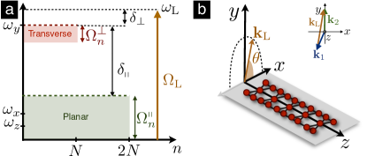
Figure 2: Vibrational modes of the ladder compounds: (a) Schematic representation of the phonon branches, whereby the transverse vibrational frequencies $\Omega_{n}^{\bot}$ span around the trap frequency $\omega_{y}$, and are situated far away from the planar phonon branch $\Omega_{n}^{\shortparallel}$, which spans around $\omega_{x},\omega_{z}$. (b) Laser beam arrangement (inset) for a spin-dependent dipole force with an effective wavevector ${\bf k}_{\rm L}$ in the $xy$-plane slightly tilted from the $y$-axis. The effective frequency $\omega_{\rm L}$ is tuned above the resonance of the transverse modes (see (a)), such that the detunings fulfill $\delta_{\shortparallel}\gg\delta_{\bot}$.

II.3 State-dependent dipole forces

The use of the collective vibrational modes as a common data bus to perform two-qubit gates can also be understood in terms of phonon-mediated spin-spin interactions ions_ising_interaction , which opens the route towards the QS of quantum magnetism ising_porras ; spin_models_ti . We now introduce the key ingredient for such QSs, namely, a spin-phonon coupling that originates from a laser-induced state-dependent dipole force sd_force ; sd_force_review .

So far, our discussion applies to all ion species and radio-frequency traps. However, in order to exploit the phonons as mediators of a spin-spin interaction that is sufficiently strong, the trap frequencies for each particular ion species must be tuned such that $l_{z}=(e^{2}/m\omega_{z}^{2})^{1/3}\approx 1$-10 $\mu$m, and $\omega_{y}\gg\omega_{x}\geq\omega_{z}$. This typically constraints the order of magnitude of the trap frequencies to the range $\omega_{z}/2\pi,\omega_{x}/2\pi\approx$ 0.1-1 MHz, and $\omega_{y}/2\pi\approx$ 1-10 MHz. Moreover, since we aim at a flexible control of the anisotropy of the spin couplings, we shall focus on the ion species that allow for a two-photon lambda scheme to implement the spin-phonon coupling. Hence, our discussion will be specific to singly ionized alkaline-earth ions, either with a hyperfine structure ${}^{9}{\rm Be}^{+}$, ${}^{25}{\rm Mg}^{+}$, and ${}^{43}{\rm Ca}^{+}$, or with a pair of Zeeman-split levels such as ${}^{40}{\rm Ca}^{+}$ and ${}^{24}{\rm Mg}^{+}$ note_optical .

In Fig. 3, we represent schematically the atomic energy levels of such ions, which have a single valence electron in the orbital $n\hskip 2.15277pt^{2}S_{1/2}$ that can be optically excited to $n\hskip 2.15277pt^{2}P_{1/2},n\hskip 2.15277pt^{2}P_{3/2}$ via a dipole-allowed transition. Here, we use the standard notation $n\hskip 2.15277pt^{2S+1}L_{J}$, with $n$ as the principal quantum number, and $S,L,J$ as the spin, orbital, and total electronic angular momentum. Depending on the nuclear spin $I$ of the particular ion, the ground-state manifold will be split into a pair of Zeeman states ($I=0$), or a set of hyperfine levels ($I\neq 0$). We select two of such states $|{\uparrow_{i}}\rangle,|{\downarrow_{i}}\rangle$, which are separated by an energy gap $\omega_{0}$, to form the effective spins of our QS (see the inset of Fig. 3). For hyperfine spins, the energy splitting is $\omega_{0}/2\pi\approx$ 1-10 GHz, whereas for Zeeman spins its order of magnitude depends on the external magnetic field $\omega_{0}/B_{0}\approx 2\pi\times$10 GHz/T.

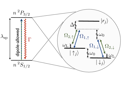
Figure 3: Lambda scheme for the dipole force: Two electronic states $\{|\uparrow_{j}\rangle,|\downarrow_{j}\rangle\}$ with an energy difference $\omega_{0}$ are selected from the ground-state manifold $n^{2}S_{1/2}$ to form an effective spin-1/2. These states can be manipulated by a pair of laser beams with Rabi frequencies $\Omega_{1,\sigma},\Omega_{2,\sigma}$ that induce a transition to an excited state $|r_{j}\rangle$ in the $n^{2}P_{3/2}$ manifold from the spin state $s=\uparrow,\downarrow$ in $n^{2}S_{1/2}$. Note that the transition wavelength $\lambda_{\rm sp}$ lies in the optical regime. When the beatnote $\omega_{\rm L}=\omega_{1}-\omega_{2}$ is tuned close to the trap frequency $\omega_{y}$, such that the detuning $\Delta$ is much larger than the spontaneous decay rate $\Gamma$ of the transition and the Rabi frequencies, one obtains the desired state-dependent dipole force.

Accordingly, the resonance frequencies usually lie in the radio-frequency/microwave regime. However, it is not customary to use radio-frequency/microwave radiation to couple the spins to the collective vibrational modes, since its wavelength is much larger than the typical ion oscillations (but see the recent experimental progress microwaves ). A possible alternative is to use a pair of laser beams with optical frequencies $\omega_{1},$ $\omega_{2}$, a ”moving standing wave”, to induce a two-photon stimulated Raman transition through an excited state $|r_{i}\rangle$ (see Fig. 3). When the laser beams are far off-resonant with respect to this dipole-allowed transition, such that the detuning $\Delta$ is much larger than the decay rate of the excited state $\Gamma$ and the laser Rabi frequencies $\Omega_{1,s},\Omega_{2,s}$, where $s=\uparrow,\downarrow$, it is possible to eliminate the excited state from the dynamics and obtain a Hamiltonian that only involves the spins and the phonons (see Appendix A for the effective master equation). In particular, when the laser beatnote is $\omega_{\rm L}=\omega_{1}-\omega_{2}\approx\omega_{y}\ll\omega_{0}\ll\Delta$ (Fig. 2(a)), one obtains the following ion-laser Hamiltonian

$$H_{\rm d}=\frac{\Omega_{\rm L}}{2}\sum_{i}\sigma_{i}^{z}{\rm e}^{{\rm i}{\bf k}_{\rm L}\cdot{\bf r}^{0}_{i}}{\rm e}^{{\rm i}({\bf k}_{\rm L}\cdot\Delta{\bf r}_{i}-\omega_{\rm L}t)}+\text{H.c.},$$ (10)

which can be interpreted as a time-dependent differential ac-Stark shift due to the interference of the two laser beams. Here, we have introduced $\sigma_{i}^{z}=|{\uparrow_{i}}\rangle\langle{\uparrow_{i}}|-|{\downarrow_{i}}\rangle\langle{\downarrow_{i}}|$, and the two-photon differential Rabi frequency $\Omega_{\rm L}=(\Omega_{\rm 1,\downarrow}^{\phantom{*}}\Omega_{\rm 2,\downarrow}^{*}-\Omega_{\rm 1,\uparrow}^{\phantom{*}}\Omega_{\rm 2,\uparrow}^{*})/2\Delta$. The corrections due to the spontaneous decay from the excited level contribute to the Rabi frequency with $\Omega_{\rm L}\to\Omega_{\rm L}(1+(\Gamma/\Delta)^{2})$, and can be thus neglected if $\Gamma\ll\Delta$.

The idea is that by controlling experimentally the polarizations, intensities and detunings of the laser beams, one can find regimes where the effective Rabi frequency $\Omega_{\rm L}$ does not vanish and leads to a spin-dependent dipole force. Let us note that the adiabatic elimination also leads to standard ac-Stark shifts and to a running wave that only couples to the vibrational excitations. These terms must be compensated by carefully selecting the laser-beam parameters. Let us finally emphasize that the effective Raman wavevector ${\bf k}_{\rm L}={\bf k}_{1}-{\bf k}_{2}=k_{\rm L}\cos\theta{\bf e}_{x}+k_{\rm L}\sin\theta{\bf e}_{y}$ has a component along the ladder plane (see Fig. 2(b)), and in principle couples to both the planar and transverse phonons. The reason for the announced decoupling from the planar vibrational modes is that the beatnote of the laser beams, which is near the resonance of the transverse phonons, will lie far off-resonance with respect to the planar vibrational modes (Fig. 2(a)). This qualitative argument will be quantified below, and supported numerically in Sec III.

After introducing the phonon operators in Eq. (7), we perform a Taylor expansion of Eq. (10) for the small transverse and planar Lamb-Dicke parameters

$$\eta_{n\bot}=\frac{k_{{\rm L}}\sin\theta}{\sqrt{2m\Omega_{n}^{\bot}}}\ll 1,\hskip 8.61108pt\eta_{n\shortparallel}=\frac{k_{{\rm L}}\cos\theta}{\sqrt{2m\Omega_{n}^{\shortparallel}}}\ll 1.$$ (11)

By setting $\omega_{\rm L}\gtrsim\omega_{y}$, such that the bare detuning fulfills $|\delta_{y}|=|\omega_{y}-\omega_{\rm L}|\ll|\delta_{x}|=|\omega_{x}-\omega_{L}|,\omega_{y}$, one can neglect all non-resonant terms apart from a state-dependent dipole force that couples the spins to the transverse phonons. In the interaction picture with respect to the phonon Hamiltonian (9), we get

$$H_{\rm d}=\frac{\Omega_{\rm L}}{2}\sum_{i,n}{\rm i}{\rm e}^{{\rm i}{\bf k}_{\rm L}\cdot{\bf r}_{i}^{0}}\eta_{n\bot}\mathcal{M}_{in}^{\bot}\sigma_{i}^{z}a_{n}^{\dagger}{\rm e}^{{\rm i}\delta_{n\bot}t}+\text{H.c.},$$ (12)

where $\delta_{n\bot}=\Omega_{n}^{\bot}-\omega_{\rm L}$. We note that, in order to neglect all the remaining terms of the Taylor expansion, a rotating wave approximation (RWA) must be performed, provided that

$$\frac{\Omega_{\rm L}}{\omega_{\rm L}}\ll 1,\hskip 8.61108pt\frac{\eta_{n\shortparallel}\Omega_{\rm L}}{|\Omega_{n}^{\shortparallel}-\omega_{\rm L}|}\ll\frac{\eta_{n\bot}\Omega_{\rm L}}{|\Omega_{n}^{\bot}-\omega_{\rm L}|}.$$ (13)

The first condition is required to neglect the off-resonant contributions to the ac-Stark shift of the energy levels. Additionally, by virtue of Eq. (11), this condition ensures that the spin-phonon couplings involving higher-order powers of the transverse phonon operators can also be neglected. For the regime considered in this work, namely $\omega_{\rm L}\approx\omega_{y}\gg\omega_{x}\geq\omega_{z}$, it will suffice to consider $\Omega_{\rm L}/2\pi\leq$ 0.1-1 MHz to accomplish this constraint. The second condition in (13) is necessary to avoid that the dipole force also couples the spins to the planar phonons. Hence, it characterizes the parameter regime where our previous qualitative discussion about the decoupling of the planar vibrational modes holds. The fulfillment of this condition relies on the large gap between the frequencies of the transverse and planar normal modes. Besides, by setting the laser-beam arrangement such that $\theta\approx\pi/2$, one obtains $\eta_{n\shortparallel}\ll 1$, which warrants the fulfillment of the last condition. In Sec. III, we will confirm the validity of these constraints numerically for the particular case of a zigzag ion ladder.

Depending on the spin state, the dipole force in Eq. (12) pushes the ions in opposite directions transversally to the ladder plane. Besides, the phase of this pushing force depends on the ratio of the ion equilibrium positions and the effective wavelength of the interfering laser beams. As shown below, this is precisely the parameter that shall allow us to control the anisotropy of the effective spin-spin couplings.

II.4 Spin models with tunable anisotropy and frustration

There are numerous situations in nature where interactions are mediated by the exchange of particles. Of particular relevance to the field of magnetism is the so-called Ruderman-Kittel-Kasuya-Yosida (RRKY) mechanism rkky , whereby a Heisenberg coupling between distant nuclear spins is mediated by electrons from the conduction band of a metal. The sign of the Heisenberg couplings alternates between ferromagnetic/antiferromagnetic as a function of the ratio between the Fermi wavelength and the mutual spin distance. We have recently shown frustration_ulm that a similar phenomenon occurs for trapped-ion ladders subjected to the dipole force in Eq. (12). Instead of a Heisenberg-type interaction between the nuclear spins, one obtains a periodically-modulated Ising-type coupling between the spins formed by two electronic states of the ion. Interestingly enough, the modulation can be experimentally tailored by controlling the direction of propagation of the interfering laser beams providing the dipole force.

The Ising interaction between the effective spins of two distant ions can be understood as a consequence of the virtual phonon exchange between these ions. The dipole force (12) pushes the ions transversally, exciting thus the transverse vibrational modes. These phonon excitations, being collective, can be reabsorbed elsewhere in the ion crystal, providing a mechanism to couple the distant spins. The exact expression can be obtained by a Lang-Firsov-type transformation comment ; polaron_book ; kanamori ; elliot ; spin_displacement_wunderlich ; ising_porras that decouples the spins from the phonons

$$U_{S}={\rm e}^{S},\hskip 8.61108ptS=\frac{\Omega_{\rm L}}{2}\sum_{i,n}{\rm i}{\rm e}^{{\rm i}{\bf k}_{\rm L}\cdot{\bf r}_{i}^{0}}\frac{\eta_{n\bot}}{\delta_{n}^{\bot}}\mathcal{M}_{in}^{\bot}\sigma_{i}^{z}a_{n}^{\dagger}-\text{H.c.}$$ (14)

This canonical transformation leads to an effective Hamiltonian $U^{\dagger}_{S}(\tilde{H}_{\rm p}+\tilde{H}_{\rm d})U_{S}\approx\tilde{H}_{\rm eff}+\tilde{H}_{\rm p}$, where we consider a picture such that the vibrational Hamiltonian $H_{\rm p}$ (9) absorbs the time-dependence of the dipole force $H_{\rm d}$ (12), namely $|\tilde{\psi}(t)\rangle=U(t)|\psi(t)\rangle$, where $U(t)={\rm exp}({{\rm i}t\sum_{n}\omega_{\rm L}a_{n}^{\dagger}a_{n}^{\phantom{\dagger}}})$. This leads to the following representation of the total Hamiltonian

$$\tilde{H}_{\rm p}+\tilde{H}_{\rm d}=\sum_{n}\delta_{n}^{\bot}a_{n}^{\dagger}a_{n}^{\phantom{\dagger}}+\frac{\Omega_{\rm L}}{2}\sum_{i,n}({\rm i}{\rm e}^{{\rm i}{\bf k}_{\rm L}\cdot{\bf r}_{i}^{0}}\eta_{n\bot}\mathcal{M}_{in}^{\bot}\sigma_{i}^{z}a_{n}^{\dagger}+\text{H.c.}).$$ (15)

After applying the above Lang-Firsov-type transformation, and moving back to the original Schrödinger picture, we obtain the following effective Ising model

$${H}_{\rm eff}=\sum_{i}\sum_{j\neq i}J_{ij}^{\rm eff}\sigma_{i}^{z}\sigma_{j}^{z}.\\$$ (16)

The effective spin couplings have the following expression

$$J_{ij}^{\rm eff}=-\sum_{n}\frac{\Omega_{\rm L}^{2}k_{\rm L}^{2}\sin^{2}\theta}{8m\Omega_{n}^{\bot}\delta_{n\bot}}\mathcal{M}_{in}^{\bot}\mathcal{M}_{jn}^{\bot}\cos({\bf k}_{\rm L}\cdot{\bf r}_{ij}^{0})$$ (17)

As announced previously, the phase dependence of the dipole force (12) on the ratio of the ion equilibrium positions and the effective wavelength of the light has been translated in the particular periodic modulation of the interaction strengths $J_{ij}^{\rm eff}\propto\cos({\bf k}_{\rm L}\cdot{\bf r}_{ij}^{0})$. This sign alternation is similar to that found in RKKY metals, such that the transverse phonons play the role of the conduction electrons, and the wavelength of the interfering laser beams acts as the Fermi wavelength. In the regime of interest for the ladders, $\kappa_{y}\ll 1$, the couplings

$$J_{ij}^{\rm eff}=\frac{J_{\rm eff}\cos\phi_{ij}}{|{\bf\tilde{r}}_{i}^{0}-{\bf\tilde{r}}_{j}^{0}|^{3}},$$ (18)

display a dipolar decay law, where we have introduced

$$J_{\rm eff}=\frac{\Omega_{\rm L}^{2}\eta_{y}^{2}}{8\delta_{y}^{2}}\kappa_{y}\omega_{y},\hskip 8.61108pt\phi_{ij}=2\pi\frac{l_{z}(\tilde{x}_{i}^{0}-\tilde{x}_{j}^{0})\cos\theta}{\lambda_{\rm L}},$$ (19)

such that $\eta_{y}=k_{\rm L}\sin\theta/\sqrt{2m\omega_{y}}$ is the bare Lamb-Dicke parameter. From these expressions, it becomes apparent that the interactions between spins belonging to the same leg of the ion ladder ($\phi_{ij}=0$) correspond to antiferromagnetic $J^{\rm eff}_{ij}>0$ Ising couplings. Conversely, the interactions between the spins from different legs of the ladder ($\phi_{ij}\neq 0$) can be ferromagnetic $J^{\rm eff}_{ij}<0$ or antiferromagnetic $J^{\rm eff}_{ij}>0$ depending on the laser parameters. We can thus tune the sign and magnitude of the spin-spin couplings anisotropically. Note that, even if the typical optical wavelengths are much smaller than the mutual ion distances $\lambda_{\rm L}\ll l_{z}\approx 1$-10 $\mu$m, the angle $\theta$ can be tuned around $\theta\approx\frac{\pi}{2}$ so that $\phi_{ij}$ attains any desired value $\phi_{ij}\in[0,2\pi]$. Alternatively, it is also possible to maintain the laser-beam arrangement fixed, and modify the anisotropy ratio $\kappa_{x}=(\omega_{z}/\omega_{x})^{2}$ in order to control the inter-ion distances $\tilde{x}_{i}^{0}-\tilde{x}_{j}^{0}$, attaining thus the desired value $\phi_{ij}\in[0,2\pi]$. Either of these two methods will turn out to be essential to explore the full phase diagram of the frustrated quantum spin ladders.

This anisotropy of the model leads to frustration when

$$\mathcal{F}_{P}=\text{sign}\left\{\prod_{(i,j)\in{P}}-J^{\text{eff}}_{ij}\right\}=-1,$$ (20)

where $P$ stands for the elementary plaquette of the lattice, which is a triangle in our case $\mathcal{F}_{\triangle}=-1$ (see Figs. 1(b),(c) and (e)). Therefore, the Ising model is frustrated if there is an odd number of antiferromagnetic couplings per unit cell. We note that this standard criterion of geometric frustration villain_frustration can be extended to situations where quantum fluctuations and frustration have the same source frustration_criteria . In our case, however, the frustration is purely classical, interpolating between the antiferromagnetic frustration, and the frustration due to competing ferromagnetic and antiferromagnetic interactions. In order to introduce quantum fluctuations, a microwave directly coupled to the atomic transition yields

$${H}_{\rm eff}=\sum_{i}\sum_{j\neq i}J_{ij}^{\rm eff}\sigma_{i}^{z}\sigma_{j}^{z}-h\sum_{i}\sigma_{i}^{x},$$ (21)

where we have introduced $\sigma_{i}^{x}=|{\uparrow_{i}}\rangle\langle{\downarrow_{i}}|+|{\downarrow_{i}}\rangle\langle{\uparrow_{i}}|$, and $h$ plays the role of an effective transverse field of strength $h$ due to the microwave, which is responsible for the quantum fluctuations.

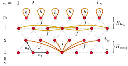
Figure 4: Anisotropic spin-spin interactions: The legs of the trapped-ion ladder are labeled by the index $\gamma=1,\dots,n_{\rm l}$, whereas the spins in each leg correspond to $i_{\rm s}=1,\dots,L_{\gamma}$. The effective spin ladder hamiltonian is composed of two terms: $H_{\rm leg}$ contains single-spin terms corresponding to the transverse field $h\lessgtr 0$ (yellow-red laces) and the antiferromagnetic dipolar couplings $J>0$ (yellow bonds). $H_{\rm rung}$ contains the couplings between spins of different rungs, such that $\tilde{J}\lessgtr$ (yellow-red bonds) depends on the mutual rung distance $d_{\gamma\mu}$. We also show the unit vectors ${\bf a}_{1},{\bf a}_{2}$ of the triangular lattice.

Let us close this section by rewriting the effective anisotropic quantum Ising model (21) in a notation that is more appropriate for quantum spin ladders (see Fig. 4). We substitute the label of the spins $i=1,\cdots,N$ for two new indices that account for the number of legs $\gamma=1,\cdots,n_{\rm l}$, and the number of spins in each of these legs $i_{\rm s}=1,\cdots,L_{\gamma}$, such that $\sum_{\gamma}L_{\gamma}=N$. Then, the Hamiltonian can be rewritten as $H_{\rm eff}=H_{\rm leg}+H_{\rm rung}$, where the leg and rung Hamiltonians are

$$\begin{split}H_{\rm leg}&=\sum_{\gamma}\sum_{i_{\rm s}\neq j_{\rm s}}J^{\gamma}_{i_{\rm s},j_{\rm s}}\sigma_{i_{\rm s}}^{z}(\gamma)\sigma_{j_{\rm s}}^{z}(\gamma)-h\sum_{\gamma}\sum_{i_{\rm s}}\sigma_{i_{\rm s}}^{x}(\gamma),\\ H_{\rm rung}&=\sum_{\gamma\neq\mu}\sum_{i_{\rm s}\neq j_{\rm s}}\tilde{J}_{i_{\rm s},j_{\rm s}}^{\gamma,\mu}\sigma_{i_{\rm s}}^{z}(\gamma)\sigma_{j_{\rm s}}^{z}(\mu).\\ \end{split}$$ (22)

Here, we have introduced the intra- and inter-leg Ising coupling strengths, which are respectively

$$\begin{split}J_{i_{\rm s},j_{\rm s}}^{\gamma}&=\frac{J_{\rm eff}}{|{\bf\tilde{r}}_{i_{\rm s}}^{0}(\gamma)-{\bf\tilde{r}}^{0}_{j_{\rm s}}(\gamma)|^{3}},\\ \tilde{J}_{i_{\rm s},j_{\rm s}}^{\gamma,\mu}&=\frac{\tilde{J}_{\rm eff}}{|{\bf\tilde{r}}_{i_{\rm s}}^{0}(\gamma)-{\bf\tilde{r}}^{0}_{j_{\rm s}}(\mu)|^{3}},\end{split}$$ (23)

where $\tilde{J}_{\rm eff}=J_{\rm eff}\cos\tilde{\phi}_{\gamma\mu}$, such that $\tilde{\phi}_{\gamma\mu}=k_{\rm L}\cos\theta d_{\gamma\mu}$, and $d_{\gamma\mu}$ is the inter-leg distance (see Fig. 4). These are the central equations of this manuscript, describing a general $n_{\rm l}$-leg quantum Ising ladder, whereby the each of the legs corresponds to an antiferromagnetic quantum Ising chain with long-range dipolar interactions. The one-dimensional chains are coupled by means of dipolar Ising pairwise interactions with a strength and sign that can be experimentally controlled. In particular, we shall be interested in a ferromagnetic coupling that competes with the intra-leg antiferromagnetic interactions, leading thus to the phenomenon of magnetic frustration.

At this point, it is worth commenting on the interesting recent proposal arbitrary_lattice for the simulation of any network of $N$ interacting spins by using a linear crystal of ions. By exploiting $N$ different laser beams individually addressed to each ion, such that the detunings and Rabi frequencies are fine tuned, it is possible to synthesize the connectivity of any desired network. Our approach is different since it exploits the specific geometry of self-organized planar ion crystals, and can be scaled to large ion ensembles straightforwardly. Additionally, it benefits from the simplicity of using a single laser-induced dipole force that lies far off-resonance from the whole vibrational branch. This contrasts the proposal in arbitrary_lattice , where the forces lie within the vibrational branch, and resonance effects must be carefully avoided for larger ion chains where the phonon branches become denser. We note that the scheme in arbitrary_lattice has a higher flexibility in the simulated lattices, although the geometry of the ladders in our approach can be partially modified following the prescriptions of Sec. IV.

In the following section, we support the validity of this analytical treatment with a numerical study of the zigzag ladder.

III A Detailed Case: The Zigzag Ladder

III.1 Numerical support for the anisotropic Ising model

We consider the simplest scenario where the anisotropy of the Ising model can be tested, namely, a three-ion chain in a zigzag configuration. We consider the following guiding numbers for the trap frequencies $\omega_{y}/\omega_{z}=20,\omega_{x}/\omega_{z}=1.43$, and $\omega_{z}/2\pi=1$ MHz, although we emphasize that the scheme will equally work for different values as far as the above constraints are met. These values lead to the equilibrium positions

$$\tilde{{\bf r}}_{i}^{0}\in\{(-0.22,0,-0.92),(0.44,0,0),(-0.22,0,0.92)\}.$$ (24)

We focus on the crucial assumption that allows us to derive the effective frustrated Hamiltonian (21), namely the possibility to neglect the pushing force on the planar modes. To address the validity of this approximation, we start from the vibrational Hamiltonian in Eq. (3), and introduce the creation-annihilation operators for the local ion vibrations

$$\Delta r_{i\alpha}=\frac{1}{\sqrt{2m\omega_{\alpha}}}\bigg{(}a_{i\alpha}^{\phantom{\dagger}}+a_{i\alpha}^{\dagger}\bigg{)},\hskip 4.30554ptp_{i\alpha}={\rm i}\sqrt{\frac{m\omega_{\alpha}}{2}}\bigg{(}a_{i\alpha}^{\dagger}-a_{i\alpha}^{\phantom{\dagger}}\bigg{)}.$$ (25)

Even if the state-dependent dipole coupling in Eq. (10) only acts along the $xy$ plane, the motion along the $z$-axis gets coupled through the Coulomb interaction (6). Therefore, we must treat the complete vibrational Hamiltonian

$$\begin{split}H_{1}=&\sum_{i}\sum_{\alpha=x,y,z}\omega_{\alpha}\big{(}a_{i\alpha}^{\dagger}a_{i\alpha}^{\phantom{\dagger}}+\textstyle\frac{1}{2}\big{)}+\\ +&\frac{\omega_{z}}{4}\sum_{\alpha,\beta}\sum_{i,j}(\kappa_{\alpha}\kappa_{\beta})^{1/4}\mathcal{\tilde{V}}_{ij}^{\alpha\beta}(a_{i\alpha}^{\phantom{\dagger}}+a_{i\alpha}^{\dagger})(a_{j\beta}^{\phantom{\dagger}}+a_{j\beta}^{\dagger}).\end{split}$$ (26)

The state-dependent dipole force can also be written in this local basis, yielding the following Hamiltonian

$$H_{2}={\rm i}\frac{\Omega_{\rm L}}{2}\sum_{i}\sum_{\alpha=x,y}{\rm e}^{{\rm i}{\bf k}_{\rm L}\cdot{\bf r}^{0}_{i}}\eta_{\alpha}\sigma_{i}^{z}a^{\dagger}_{i\alpha}{\rm e}^{-{\rm i}\omega_{\rm L}t}+\text{H.c.},$$ (27)

where $\eta_{\alpha}=k_{{\rm L\alpha}}/\sqrt{2m\omega_{\alpha}}$ are the bare Lamb-Dicke factors.

In order to integrate numerically the Schrödinger equation for the timescales of interest $t_{\rm f}\approx 1/|J_{\rm eff}|$, which are three orders of magnitude larger than the timescale set by the dynamics of the dipole force $1/\omega_{\rm L}$, it would be desirable to work in a picture that absorbs the fast time-dependence of (27). This is possible if we neglect the counter-rotating terms of Eq. (26) that correspond to phonon non-conserving processes, which is justified by a rotating-wave approximation when

$$\frac{\omega_{z}}{4}(\kappa_{\alpha}\kappa_{\beta})^{1/4}\mathcal{\tilde{V}}_{ij}^{\alpha\beta}\ll(\omega_{\alpha}+\omega_{\beta}).$$ (28)

Then, it is possible to move to a picture where the creation-annihilation operators rotate with the laser frequency, $|\tilde{\psi}(t)\rangle={\rm exp}({{\rm i}t\sum_{\alpha i}\omega_{\rm L}a_{i\alpha}^{\dagger}a_{i\alpha}^{\phantom{\dagger}}})|\psi(t)\rangle$, and the Hamiltonian that will be numerically explored $\tilde{H}=\tilde{H}_{1}+\tilde{H}_{2}$ becomes time-independent, namely

$$\begin{split}\tilde{H}_{1}&=\sum_{i,\alpha}\delta_{\alpha}a_{i\alpha}^{\dagger}a_{i\alpha}^{\phantom{\dagger}}+\frac{\omega_{z}}{2}\sum_{\alpha,\beta}\sum_{i,j}(\kappa_{\alpha}\kappa_{\beta})^{1/4}\mathcal{\tilde{V}}_{ij}^{\alpha\beta}a_{i\alpha}^{\dagger}a_{j\beta}^{\phantom{\dagger}},\\ \tilde{H}_{2}&={\rm i}\frac{\Omega_{\rm L}}{2}\sum_{i}\sum_{\alpha=x,y}{\rm e}^{{\rm i}{\bf k}_{\rm L}\cdot{\bf r}^{0}_{i}}\eta_{\alpha}\sigma_{i}^{z}a^{\dagger}_{i\alpha}+\text{H.c.}.\end{split}$$ (29)

Note that this unitary transformation does not affect the spin dynamics, and is thus well-suited to study the validity of our previous derivation of the effective Ising model.

In order to account for two sources of noise that are usually the experimental limiting factors for spin-oriented QSs, we include a fluctuation of the atomic resonance frequency

$$\tilde{H}_{3}=\sum_{i}\textstyle\frac{1}{2}\Delta\epsilon(t)\sigma_{i}^{z},$$ (30)

where $\Delta\epsilon(t)$ is a stochastic process. This term may correspond to the Zeeman shift of non-shielded fluctuating magnetic fields, or to a non-compensated ac-Stark shift caused by fluctuating laser intensities. Its dynamics can be modeled as a stationary, Markovian, and Gaussian process ou_process , as follows

$$\Delta\epsilon(t+\delta t)=\Delta\epsilon(t){\rm e}^{-\frac{\delta t}{\tau}}+\big{[}\textstyle{\frac{c\tau}{2}}(1-{\rm e}^{-\frac{2\delta t}{\tau}})\big{]}^{\frac{1}{2}}n_{\rm g},$$ (31)

where $n_{\rm g}$ is a unit Gaussian random variable, and $c,\tau$ characterize the diffusion constant and the correlation time of the noise. For short correlation times $\tau\ll t$, one obtains an exponential damping of the coherences with a typical time $T_{2}=2/c\tau^{2}$. We set $\tau=0.1T_{2},$ and $T_{2}\approx 10$ ms, which is a reasonable estimate for the observations in experiments. Note that this dephasing timescale still allows for the observation of the faster coherent spin dynamics $1/J^{\rm eff}_{ij}\approx 1$ ms $\ll T_{2}$.

We study numerically the time evolution under the total Hamiltonian $\tilde{H}=\sum_{m}\tilde{H}_{m}$ in Eqs. (29)-(30), and compare it to the effective description $H_{\rm eff}$ for a vanishing transverse-field in Eq. (21). We note that the following numerical simulations focus on a ground-state-cooled crystal, where the nine vibrational modes have one excitation at most. To consider the dephasing noise, we integrate over $N=10^{3}$ different histories of the fluctuating frequency (31), and perform the statistical average of the dynamics. The effects of finite temperatures, together with other error sources, are addressed in Sec. IV. To observe a neat hallmark of the anisotropy due to the modulation of the interaction strengths $J^{\rm eff}_{ij}\propto\cos({\bf k}_{\rm L}\cdot{\bf r}_{ij}^{0})$, we study the dynamics of the spin state $|\psi_{\rm s}\rangle=|+\rangle_{1}\otimes|-\rangle_{2}\otimes|-\rangle_{3}$, where $|\pm\rangle=(|\uparrow\rangle\pm|\downarrow\rangle)/\sqrt{2}$, for two sets of parameters.

(i) Allowed spin hopping: We set the following parameters $\eta_{y}=0.1=10\eta_{x}$, $\omega_{\rm L}=1.1\omega_{y}$, and $\Omega_{\rm L}=0.15|\delta_{y}|/\eta_{y}$, and direct the laser beams so that $\theta=\pi/2$ (i.e. ${\bf e}_{x}\cdot{\bf k}_{\rm L}=0$). In this case, the interfering radiation does not propagate along the triangle plane, and there is no modulation of the sign of the couplings. We observe that the initial spin excitation $|+\rangle$ located at site 1, can tunnel to the two remaining sites of the triangular plaquette as a consequence of the Ising-like coupling. In Fig. 5(a), we compare the numerical results with the effective description. From this figure, we can conclude that the effective Ising Hamiltonian yields an accurate description of the spin dynamics in a timescale $t_{\rm f}\approx 1/J_{\rm eff}$- $2/J_{\rm eff}\approx 1$-$2$ ms$<T_{2}\approx 10$ ms. For longer timescales, the dephasing leads to a larger deviation from the effective description. Note that this result supports the validity of the isotropic Ising interaction, but we still have to address whether our scheme to control interaction anisotropy is also accurate.

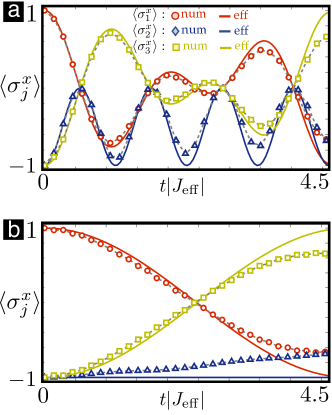
Figure 5: Spin dynamics in the triangular plaquette: (a) Dynamics of an initial spin excitation $|+\rangle_{1}$ in the allowed-hopping regime. The dynamics of $\langle\sigma_{j}^{x}(t)\rangle$ obtained from the effective description $H_{\rm eff}$ ($\langle\sigma_{1}^{x}(t)\rangle$ red line, $\langle\sigma_{2}^{x}(t)\rangle$ blue line, $\langle\sigma_{3}^{x}(t)\rangle$ yellow line) show a remarkable agreement with the numerical simulation of the complete Hamiltonian $\tilde{H}$ ($\langle\sigma_{1}^{x}(t)\rangle$ red circles, $\langle\sigma_{2}^{x}(t)\rangle$ blue triangles, $\langle\sigma_{3}^{x}(t)\rangle$ yellow squares), and both describe the transport of the spin excitation around the plaquette. (b) In the inhibited hopping regime, one also observes a complete agreement between both descriptions, which describe how the spin excitation cannot occupy site $2$ as a consequence of the vanishing Ising interaction.

(ii) Inhibited spin hopping: We use the same parameters as before, but now consider that the interfering laser radiation also propagates along the plane defined by the triangle. In particular, we set the angle and the effective wavelength as follows $\lambda_{\rm L}/\cos\theta=4l_{z}(\tilde{x}_{1}^{0}-\tilde{x}_{2}^{0})=4l_{z}(\tilde{x}_{3}^{0}-\tilde{x}_{2}^{0})$, which leads to the factors $\phi_{12}=\phi_{32}=\pi/2$, such that the effective Ising couplings between sites $1$-$2$ and $2$-$3$ completely vanish $J_{12}^{\rm eff}=J_{23}^{\rm eff}=0$. Therefore, we reach a highly anisotropic situation where the spin excitation can only hop between sites $1\leftrightarrow 3$. This is confirmed by the numerical results in Fig. 5(b), where a good agreement with the effective description is displayed once more in the timescale $t_{\rm f}\approx 1$-$2$ ms.

Let us finally stress that an experiment with three ions in this triangule would be a neat proof-of-principle to show that anisotropic Ising models can be realized following our scheme. We also stress that this scheme is amenable of being scaled to larger systems, since the periodically modulated couplings are controlled globally by the ratio of the laser wavelength to the inter-leg equilibrium positions, and thus does not depend critically on the size of the Coulomb crystal.

III.2 Frustration by competing interactions

Once the validity of the effective Ising model (21) has been numerically supported, we can exploit the anisotropic interactions (17) to interpolate between a frustrated Ising ladder due to antiferromagnetic couplings, or due to the competition of ferromagnetic and antiferromagnetic interactions. In Fig. 6(a), we present a scheme of the spin frustration. The intra-leg spin couplings in the ladder (yellow) correspond to antiferromagnetic interactions which, according to Eq. (17), cannot be modulated. On the other hand, the inter-leg couplings along the diagonal rungs of the ladder may correspond to antiferromagnetic (yellow) or ferromagnetic (red) interactions depending on the value of $\phi_{ij}=k_{\rm L}\cos\theta(x_{i}^{0}-x_{j}^{0})$. Both situations lead to frustration (see Fig. 6(b)), since only two of the bonds can be satisfied simultaneously. By using the normal modes of the inhomogeneous zigzag chain, we compute numerically the spin couplings, and show that for $\phi_{j_{0},j_{0}+1}=0$, we obtain an antiferromagnetic coupling (Fig. 6(c)), whereas an alternating sign arises for $\phi_{j_{0},j_{0}+1}=\pi/2$ (Fig. 6(d)).

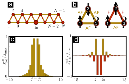
Figure 6: Spin frustration in the zig-zag ladder: (a) Scheme of the Ising interactions between neighboring ions in the zig-zag ladder, whereby the red links stand for a ferromagnetic coupling, whereas the yellow-red links can be antiferromagnetic/ferromagnetic interactions. (b) Frustration in a triangular plaquette where one of the bonds cannot be satisfied by any spin configuration (left: purely antiferromagnet, right: competing interactions). (c) Effective interaction strength between the central ion $j_{0}=N/2$ and its neighbors, as obtained from the numerical solution of Eq. (17) for $N=30$ ions in a trap with $\omega_{y}\gg\omega_{x}=6.1\omega_{z}$. For $\phi_{j_{0},j_{0}+1}=0$, one observes the dipolar decay of the frustrated antiferromagnetic interactions. (d) For $\phi_{j_{0},j_{0}+1}=\pi/2$, the sign alternation leads to competing interactions.

IV Experimental Considerations

In previous sections, we discussed the regimes of validity of the spin models by both analytic and numerical methods. Here, we analyze the capability of ion-trap experiments to meet the required conditions, considering current technology limitations and possible sources of error in ion-trap experiments. This study is supported by initial experiments.

IV.1 Trap design study

A crucial condition for the frustrated quantum spin models is $\omega_{y}\gg\omega_{x}\geq\omega_{z}$, which leads to the clustering of vibrational branches exploited in Sec. II. This condition implies that the rotational symmetry of the trap potential in the $xy$-plane, which is a common property of linear Paul traps, must be explicitly broken. In this section, we discuss two possible strategies to achieve this goal, and present supporting evidence based on numerical and experimental results.

The first approach can be implemented in any linear Paul trap, such as the symmetric electrode arrangement shown in the inset of Fig. 7(a). By applying a positive offset voltage $U_{\rm offset}$ on the DC electrodes, the trapping potential becomes stronger along the diagonal direction joining the DC electrodes, and the trapping frequencies fulfill $\omega_{y}>\omega_{x}$ (and vice versa for a negative offset voltage). For the experimental results shown in Fig. 7(a), resonant radio-frequency radiation was used to excite the different modes, such that the induced ion motion was observed on a CCD camera. This method allows for the estimation of the trap frequencies, which show a clear agreement with numerical ion-trajectory simulations numerical_tools (main panel of Fig. 7(a)). Note that the anisotropy of the radial frequencies $\omega_{x}/\omega_{y}$ can be tailored by the offset voltage, which also rotates the trap axes, and effectively changes the angle $\theta$ of the laser wavevector ${\bf k}_{\rm L}$ with the $x$-axis (see Fig. 7(a)). This pinpoints the possibility of shaping the spin frustration according to Eqs. (18)-(19) by modifying the electrode voltages, avoiding thus the more demanding modification of the laser-beam arrangement. In Fig. 8, we show the measured positions for a $N=17$ ion crystal. We show how the trap-frequency anisotropy can be exploited to synthesize a particular 3-leg ladder whose equilibrium positions match perfectly the numerical predictions.

The second strategy is to exploit a trap design with a non-quadrangular arrangement of the electrodes. This breaks directly the rotational symmetry of the trapping potential (see the inset of Fig. 7(b)). Both the experimental data, as measured by laser spectroscopy, and the numerics indicate a sizable splitting of the radial frequencies. Note that the dependence of the angle $\theta$ on the offset voltage depends strongly on the trap geometry. Unfortunately, in the present case, the region with the largest tunability of $\theta$ still coincides with the lowest radial anisotropies.

In order to optimize both effects, we have designed a new trap (Fig.7(c)) that meets with the special requirements of the QS. While the three-ion case-study may be realized with any state-of-the-art experimental setup, the larger scale QS with planar spin systems with about 50 ions, as shown in Fig. 1, will require a special trap design optimized according to the following conditions: (a) the trapping potential should be highly anisotropic $\omega_{y}\gg\omega_{x}$, (b) the trap should allow for the confinement of a large number of ions $N<$ 100, (c) trap frequencies should be high such that an initialization of the ion crystal in a low thermal motional state is possible, (d) the trap geometry should reduce excess micromotion, and (e) optical access should allow for readout of the spin state. We now discuss the methods to achieve these requirements.

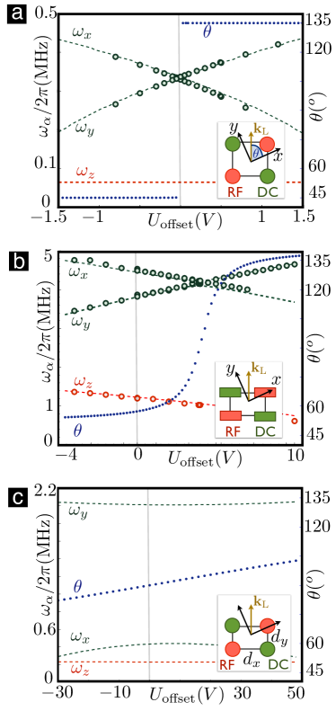
Figure 7: Experimental determination and numerical simulations of the secular frequencies in different trap geometries: Measured radial frequencies $\omega_{x},\omega_{y}$ (green dots), calculations (green dashed lines), measured axial frequency $\omega_{z}$ (red dots) and calculated values (red dashed lines) for three different trap geometries. Furthermore the angle $\theta$ (blue dots) is shown. The insets in (a)-(c) show the trap electrodes and axis seen from a radial cut through the trap. All experimental parameters match those of the simulation. Due to technical difficulties in determining the exact RF voltage we adapted its value by $\leq 10\%$. (a) Quadrangular alignment ($d_{x}=d_{y}=0.82$ mm) of the four electrodes, which leads to degenerate radial frequencies for no offset-voltage and only two possible values for $\theta$. (b) Microtrap-design as in microtrap_details with $d_{x}=125\mu$m, and $d_{y}=400\mu$m. (c) Simulated values for the new trap study, as described in the text.

The geometry for such a trap device is sketched in the inset of Fig. 7(c), where four round bars ($r=0.625\text{mm}$) form the radial trapping potential. As we choose a non-quadrangular arrangement with distances $(d_{x},d_{y})=(0.42\text{ mm, }2.90\text{ mm})$, the two simulated radial frequencies directly become non-degenerate. With a trapping drive frequency of $\Omega_{\rm rf}/2\pi=22$ MHz, and amplitude of 2.5 kV, we find a sufficiently high anisotropy $\omega_{x}/2\pi=0.43$ MHz$<\omega_{y}/2\pi=2.01$ MHz along the requirement (a). The axial confinement is generated by two endcaps seperated by a distance of 25 mm, which lead to $\omega_{z}/2\pi=0.23$ MHz with 2 kV applied on the endcaps. In this potential, a $N=4$ ion crystal undergoes the first structural transition to the zigzag configuration, and for $N>9$ the second structural transition is obtained. We have calculated the equilibrium positions and vibrational modes of a three-legged ladder of $N=19$ ions for these particular trap frequencies (Fig. 9). We note that by lowering the axial DC voltage, we can increase $N$ for different crystal structures, fulfilling the requirement (b). Let us now address condition (c). By setting the trap frequency to $\omega_{y}/2\pi=$2.01 MHz, the mean phonon numbers after Doppler cooling lie below $\bar{n}_{y}<5$. In order to have a thermal error below $1\%$ for these phonon numbers (see Eq. (91)), the spin-phonon coupling should be smaller than $\Omega_{\rm L}=0.02|\delta_{y}|/\eta_{y}$. However, this reduces the spin-spin interactions and magnetic-field noise may affect the dynamics at the corresponding long timescales. Therefore, multi-mode EIT cooling EIT_cooling to $\bar{n}_{y}=0.1$ shall allow us to keep the error rate to $1\%$, while maintaining spin-spin interactions in the kHz-regime (i.e. $\Omega_{\rm L}=0.15|\delta_{y}|/\eta_{y}$). Let us stress that the thermal error may be minimized by considering evolution times that are multiples of the detuning of the closest vibrational mode. In order to estimate the effects of the excess micromotion according to the point (d), we have estimated the $\xi_{i}$ values to be $\xi_{2i}=0$ and $|\xi_{1i}|<0.05\pi$ with the same beam angles as in Eq. (76). This should lead to relative errors on the order of 4-5%. Finally, the inter-ion distances are about 10 $\mu$m for the central ions, such that we can meet with requirement (e) via high numerical aperture optics allowing for single-site readout.

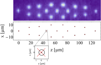
Figure 8: Three-leg ion ladder: (a) Fluorescence of a 17 ion-crystal in the trap with $\omega_{x,y,z}/(2\pi)=\left\{260,390,111\right\}\text{ kHz}$ depicted in Fig. 7 (a), inset, imaged on a CCD camera. (b) Comparison between calculated (red cross) and measured (black circle) positions show realtive errors well below one percent.

With the above parameters, the relative orientation of the ion crystal and the laser wavevector ${\bf k}_{\rm L}$ yields an angle of $\theta=\pi/2$. As discussed above, we can vary $\theta$ and tune the spin frustration by applying an offset to the DC electrodes, which rotates the crystal with respect to the fixed wavevector ${\bf k}_{\rm L}$. As shown in the simulations presented in Fig. 7(c), where the new trap design allows for a smooth tunability of $\theta$, while preserving a strong anisotropy $\omega_{x}/\omega_{y}$. With $U_{\rm offset}=-4.9$ V, we find $\omega_{x}/\omega_{y}=0.21$, while the angle becomes $\theta=0.49\pi$, already leading to a change of sign of the spin-spin coupling strength $J^{\rm eff}_{ij}$ in Eq. (19), if we assume $\lambda_{\rm L}=400$ nm.

IV.2 Tailoring the ladder geometry

In Figs. 1(b), (c) and (f), the ions self-organize naturally in a geometry of bond-sharing triangles. By controlling the number of legs in such triangular ladders, the QS is already capable of exploring a variety of interesting cooperative phenomena (see Secs. V and VI). However, it would be highly desirable to have a method to modify these geometries, widening thus the applicability of our quantum simulator.

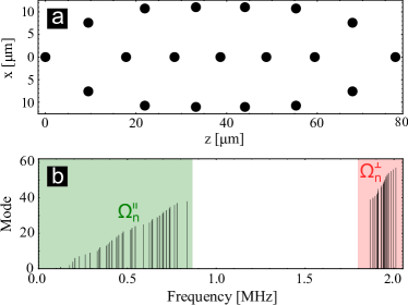
Figure 9: Vibrational modes and equilibrium positions of a three-legged ladder: (a) Equilibrium positions for a Coulomb crystal of $N=19$ ions in a Paul trap with the axial frequency $\omega_{z}/2\pi=229\text{ kHz}$ and the radial frequencies $\omega_{x}/2\pi=434$ kHz,$\omega_{y}/2\pi=2011\text{ kHz}$. The frequencies are generated by a special trap (see Fig. 7(c))design, presented in the text. (b) Vibrational modes for the same $N=19$ ion-crystal. The transverse vibrational frequencies $\Omega_{n}^{\bot}$ are clearly seperated from the planar vibrational frequencies $\Omega_{n}^{\shortparallel}$. Note the high accord with the general description in Fig. 2.

Since the geometry of the spin model (21) is determined by the couplings $J_{ij}^{\rm eff}$ between the spins $\sigma_{i}^{z}\leftrightarrow\sigma_{j}^{z}$, a possibility to tailor the geometry is to switch on/off some of these interactions. A possible route that allows for such a selective coupling is a type of laser-beam hideout. Thanks to the relatively large distances between the ions $l_{z}\approx$1-10 $\mu$m, it is possible to address them individually with laser light individual_adressing (note that the tools used so far only require global addressing). The idea is that, after the global optical pumping to the state $|\psi_{\rm s}\rangle=\otimes_{i}|\downarrow_{i}\rangle$, focused laser radiation will selectively transfer the population to a different level $|h_{i}\rangle$ that is not coupled to the spin-dependent force. Therefore, the ion gets effectively hidden. This may be achieved by polarization selection rules, or alternatively, by the ac-Stark shift of highly-detuned laser beams. Using this idea, it is possible to construct a simple ladder of corner-sharing triangles (see Fig. 1(c)), or a stripe of the two-dimensional Kagome lattice (see Fig. 1(d)). Additionally, it opens the possibility of introducing defects in the lattice in order to study the role of disorder. As discussed in Sec. V, this tool opens many possibilities for our QS.

IV.3 Imperfections and noise in the quantum simulator

Let us now address the possible sources of error in the QS. We place a special emphasis on the ion micromotion, which has not been discussed in previous QSs ising_ions ; frustration_monroe ; ising_monroe , since it can be cancelled for linear chains. We also discuss other error sources shared with the linear-chain QS, such as thermal fluctuations and heating of the phonons, dephasing of the spins, and photon scattering. We stress that, provided that the following constraints to minimize the micromotion errors are fulfilled, the proposed ladder QS should not present more limitations than its linear-chain counterparts ising_ions ; frustration_monroe ; ising_monroe .

(i) Sources of dephasing: Usually, the most important important source of error in the experiments is the dephasing of the electronic states. These might be caused by fluctuating Zeeman shifts on the magnetic-field sensitive states required to implement the spin-dependent dipole force (10); or by fluctuations in the laser-beam intensities leading to uncompensated ac-Stark shifts. A reasonable estimate of the typical coherence times $T_{2}\approx 5$-10 ms ion_trap_reviews shows that these terms are important error sources in the timescales of interest $t_{\rm f}\propto 1/J_{\rm eff}$, where $J_{\rm eff}/2\pi\approx 1$ kHz. As shown in Fig. 5, the desired coherent dynamics described by the effective Ising model (21) dominates the behavior of the system for $t_{\rm f}\approx 1$-$2$ ms. This sets the timescale for the QS of frustrated magnetism to be in the millisecond range, after which the dephasing is so strong that the quantum simulator is no longer faithful.

An interesting protocol to overcome both sources of dephasing simultaneously is based on the concept of continuous dynamical decoupling already applied to trapped ions timoney . In our case, it could be implemented by a strong driving of the carrier transition sideband_decoupling . Hence, instead of relying on the spin-dependent force (10), it suffices to combine a red-sideband term with the strong driving of the carrier. In order to obtain a quantum Ising model, one should introduce an additional microwave that provides a Zeeman shift oscillating at the Rabi frequency of the strong carrier driving. The phase diagram can be explored adiabatically by an intermediate spin-echo pulse that refocuses the fast oscillations due to the strong driving.

(ii) Role of the ion micromotion: The initial Hamiltonian in Eq. (1), upon which the derivation of the effective quantum spin ladders (22) has been built, is based on the so-called pseudo-potential approximation ion_trap_reviews . This approximation neglects the effects of the ion micromotion: a fast motion of frequency $\Omega_{\rm rf}$ that is synchronous to the radio-frequency (r.f.) field of the Paul trap. This allowed us to focus directly on the slow secular motion of the trapped ions, which is described by an effective harmonic potential (1) with frequencies $\omega_{\alpha}\ll\Omega_{\rm rf}$. The validity of this assumption is well justified for single trapped ions, where there are experimental methods to minimize the effects of the micromotion ion_trap_reviews . For linear ion chains, the micromotion is also minimized when the equilibrium positions lie along the trap axis. Conversely, for the ion ladders considered in this work, the equilibrium positions necessarily lie off the trapping axis, leading to an additional micromotion that cannot be compensated.

In Appendix B, we present a detailed discussion of the conditions under which this micromotion does not affect the QS. Let us comment on the possible sources of imperfections, and the conditions to minimize them. The r.f. heating of the transverse phonon modes responsible of the spin couplings is negligible when

$$\kappa_{y}^{1/2}|\mathcal{\tilde{V}}^{yy}_{ij}|\ll\frac{\Omega_{\rm rf}}{\omega_{z}},$$ (32)

a condition easily verified for the parameters in this work. In addition, during the cooling stage of the transverse vibrational modes, the laser frequency must be carefully tuned to avoid heating caused by the micromotion-induced broadening of the transition, or to additional micromotion sidebands micromotion_wineland .

We have also considered how the micromotion may affect the spin-dependent dipole force (10) and the spin-phonon coupling (12). To neglect the associated contributions, it is necessary to consider that the laser beams lie almost parallel to the $y$-axis, and are far off-resonant (see Fig. 3), namely $\omega_{\rm L}/2\pi\approx\omega_{y}/2\pi\approx$10 MHz$\ll\Omega_{\rm rf}/2\pi\approx 0.1$ GHz$\ll\Delta/2\pi\approx 10$ GHz. Besides, the Rabi frequencies of the laser beams should fulfill

$$|\Omega_{l,\uparrow}|,|\Omega_{l,\downarrow}|\ll\Delta,\hskip 12.91663pt\frac{|\Omega_{1,\uparrow}\Omega_{2,\downarrow}^{*}|}{2\Delta}\ll\omega_{\rm L}\ll\Omega_{\rm rf}.$$ (33)

Finally, some care must also be placed in order not to induce two-photon transitions to different states $|a_{i}\rangle$ of the atomic ground-state manifold. To avoid these processes, the relative Zeeman shifts of such transitions $\delta_{a,s}$, and the associated Rabi frequencies must be controlled such that

$$|\Omega_{1,a}\Omega_{2,s}^{*}|\ll|\delta_{a,s}-\omega_{\rm L}\pm\Omega_{\rm rf}|.$$ (34)

We thus conclude that, provided that the above restrictions on the parameters are fulfilled, the unavoidable excess micromotion of the ions in a ladder geometry should not affect our QS.

(iii) Thermal motion and heating of the ions: In Sec. III, we have supported the validity of the QS based on numerical results for ground-state cooled ion crystals. However, ever since the early schemes for phonon-mediated gates, the thermal fluctuations of the ions have been identified as a potential source of errors that must be carefully considered.

In Appendix C, we estimate the thermal error of our QS by both analytic and numerical methods. We solve exactly the Heisenberg equations of motion for the spin-dependent dipole force (15), and derive a scaling law for the thermal contribution to the $T=0$ spin dynamics, which is then supported numerically. We find that the relative thermal error, defined as $\epsilon_{T}=|\langle\sigma_{i}^{x}\rangle_{T}-\langle\sigma_{i}^{x}\rangle_{T=0}|/|\langle\sigma_{i}^{x}\rangle_{T=0}|$, has an upper bound

$$\epsilon_{T}\leq\epsilon_{\rm th}=4\frac{|\Omega_{\rm L}|^{2}\eta_{y}^{2}}{\delta_{y}^{2}}\bar{n}_{y},$$ (35)

where $\bar{n}_{y}$ represents the mean number of transverse phonons in the center-of-mass mode. By considering the parameters used in section III, the thermal fluctuations have a small contribution (1%) for $\bar{n}_{y}\approx 0.1$ (see Fig. 19), which shows that perfect ground-state cooling is not required to implement the QS accurately. At this point, we should mention that the above arguments are valid for a vanishing transverse field $h=0$. We note, however, that the contribution to the thermal error due to $h>0$ in the regime of interest $h\approx J_{\rm eff}$ has been shown ising_porras to be negligible with respect to the estimate in Eq. (35).

In Appendix C, we also present a phenomenological master equation that models possible heating mechanisms in the ion trap. We show that the relative heating error, defined as $\epsilon_{{\rm h}}=|\langle\sigma_{i}^{x}\rangle_{\Gamma_{\rm h}}-\langle\sigma_{i}^{x}\rangle_{\Gamma_{\rm h}=0}|/|\langle\sigma_{i}^{x}\rangle_{\Gamma_{\rm h}=0}|$, where $\Gamma_{\rm h}$ is the heating rate, only yields a small contribution (1%) to the overall error of the QS for heating times above 5 ms/ phonon (see Fig. 20).

(iv) Spontaneous photon scattering: The spontaneous emission can severely limit the advantage of quantum-information protocols decoherence_plenio ; photon_scattering ; photon_scattering_2 . In our case, the use of two electronic ground-states as the effective spins (see Fig. 3) makes the direct spontaneous emission $|\uparrow_{i}\rangle\rightsquigarrow|\downarrow_{i}\rangle$ negligible. However, due to the Lambda-scheme responsible for the dipole force, there can be photon scattering events from the intermediate excited state $|r_{i}\rangle$, which must be carefully considered.

In Appendix A, we describe in detail the derivation of an effective master equation ${\rm d}\rho/{\rm d}t=-{\rm i}[H_{\rm d},\rho(t)]+\mathcal{D}_{\rm eff}(\rho)$, where $H_{\rm d}$ corresponds to the dipole force (10), and

$$\mathcal{D}_{\rm eff}(\rho)=\sum_{n}\left(L^{\rm eff}_{n}\rho(L^{\rm eff}_{n})^{\dagger}-\textstyle\frac{1}{2}(L^{\rm eff}_{n})^{\dagger}L^{\rm eff}_{n}\rho-\textstyle\frac{1}{2}\rho(L^{\rm eff}_{n})^{\dagger}L^{\rm eff}_{n}\right),$$ (36)

accounts for the two possible decoherence channels. These are the so-called Raman and Rayleigh scattering of photons, and are contained in the following effective jump operators

$$\begin{split}L_{1}^{\rm eff}=\frac{\sqrt{\Gamma}}{\Delta}&\left(\Omega_{1,\downarrow}{\rm e}^{{\rm i}({\bf k}_{1}\cdot{\bf r}-\omega_{1}t)}+\Omega_{2,\downarrow}{\rm e}^{{\rm i}({\bf k}_{2}\cdot{\bf r}-\omega_{2}t)}\right)|{\downarrow}\rangle\langle{\downarrow}|+\\ +\frac{\sqrt{\Gamma}}{\Delta}&\left(\Omega_{1,\uparrow}{\rm e}^{{\rm i}({\bf k}_{1}\cdot{\bf r}-\omega_{1}t)}+\Omega_{2,\uparrow}{\rm e}^{{\rm i}({\bf k}_{2}\cdot{\bf r}-\omega_{2}t)}\right)|{\downarrow}\rangle\langle{\uparrow}|,\\ L_{2}^{\rm eff}=\frac{\sqrt{\Gamma}}{\Delta}&\left(\Omega_{1,\uparrow}{\rm e}^{{\rm i}({\bf k}_{1}\cdot{\bf r}-\omega_{1}t)}+\Omega_{2,\uparrow}{\rm e}^{{\rm i}({\bf k}_{2}\cdot{\bf r}-\omega_{2}t)}\right)|{\uparrow}\rangle\langle{\uparrow}|+\\ +\frac{\sqrt{\Gamma}}{\Delta}&\left(\Omega_{1,\downarrow}{\rm e}^{{\rm i}({\bf k}_{1}\cdot{\bf r}-\omega_{1}t)}+\Omega_{2,\downarrow}{\rm e}^{{\rm i}({\bf k}_{2}\cdot{\bf r}-\omega_{2}t)}\right)|{\uparrow}\rangle\langle{\downarrow}|,\\ \end{split}$$ (37)

where we have assumed that the scattering rate is much smaller than the laser detuning $\Gamma\ll\Delta$. Note that the first term of each jump operator does not change the spin state (i.e. Rayleigh scattering), being responsible for pure dephasing. Conversely, the second term flips the spin state (i.e. Raman scattering), leading thus to damping of the spin populations.

A conservative estimate of the photon scattering is to consider the individual effective rates (37), which scale as $\Gamma_{\rm eff}=\Gamma(|\Omega_{l,s}|/\Delta)^{2}\approx|\Omega_{\rm L}|(\Gamma/\Delta)$. By using the parameters introduced in Sec. III, we find that $\Gamma_{\rm eff}/J_{\rm eff}\approx 10^{3}(\Gamma/\Delta)$. Hence, by considering a sufficiently large detuning, it is possible to keep the scattering rates below $\Gamma_{\rm eff}/J_{\rm eff}<10^{-1}$, so that they do not compromise the accuracy of the effective description (21). For instance, for typical decay rates $\Gamma/2\pi\approx$1-10 MHz, one must consider detunings in the range $\Delta/2\pi\approx$10-100 GHz.

(v) Spatial dependence of the laser-beam profile: The effective spin couplings in Eq. (19) assume a Rabi frequency that is constant along the ion crystal. For large crystals, however, the characteristic gaussian profile for the laser intensities may lead to weaker Rabi frequencies on the boundaries of the crystal. This effect will give rise to inhomogeneous spin-spin couplings that must be added to the inhomogeneities caused by the varying inter-ion distance in Coulomb crystals. Rather than considering these terms as an error, they can be seen as a gadget that makes the many-body problem even more interesting. In particular, they will lead to inhomogeneous critical points which may be responsible of interesting effects zigzag_inhomogeneous .

IV.4 Efficient detection methods

A crucial part of a QS is the ability to perform measurements that yield information about the Hamiltonian under study. For the frustrated quantum Ising ladders (22), a QS would start by preparing the so-called paramagnetic state $|\rm P\rangle=\otimes_{i}|{\rightarrow}\rangle_{i}$ with $|{\rightarrow}\rangle_{i}=(|{\uparrow}\rangle_{i}+|{\downarrow}_{i}\rangle)/\sqrt{2}$, which is the ground-state of the model in the absence of spin interactions. Such a separable state can be accurately prepared by means of optical pumping, followed by $\frac{\pi}{2}$-pulses globally addressed to the whole ion crystal ion_trap_reviews . This step is followed by the adiabatic modification of the Hamiltonian parameters $J_{\rm eff},\tilde{J}_{\rm eff},h$, in order to connect the paramagnet to other phases of the quantum Ising ladder (see Secs. V and VI below).

A direct approach to the measurement of these phases is the so-called quantum state tomography, more precisely, the full determination of the state of the system state_tomography . However, this approach becomes highly inefficient for many-body systems due to the exponential growth of the composite Hilbert space, and alternative schemes must be studied. An interesting possibility for state estimation are the methods based on matrix-product representations of the states efficient_tomography . Another alternative that does not require full quantum state tomography is the measurement of order parameters characterizing the phases.

One of the advantages of trapped-ion experiments with respect to other platforms is their ability to perform highly-accurate measurements at the single-particle level ion_trap_reviews . The technique of state-dependent fluorescence allows for the measurement of single and joint probability distributions of the electronic states $P_{i}^{\uparrow},P_{ij}^{\uparrow\uparrow}$. From the spatially resolved fluorescence, it is possible to infer local expectation values, such as the magnetization $\langle\sigma_{i}^{z}\rangle=\frac{1}{2}(P_{i}^{\uparrow}-1)$, or two-body correlators $\langle\sigma_{i}^{z}\sigma_{j}^{z}\rangle=\frac{1}{4}[1-2(P_{i}^{\uparrow}+P_{j}^{\uparrow})+4P_{ij}^{\uparrow\uparrow}]$. As discussed in Sec. VI, these observables usually contain all the relevant information about the different phases. In particular, one could study the dependence of the correlator with the distance (48), or infer the magnetic structure factor $S_{zz}(q)=\sum_{ij}\langle\sigma_{i}^{z}\sigma_{j}^{z}\rangle{\rm e}^{{\rm i}q(i-j)}$.

Let us now comment on the possibility of recovering some of these magnitudes from global properties of the fluorescence spectrum. By measuring the probability to find a fraction of $n$-ions in the excited state $P^{\uparrow}({n})$ ising_monroe , one obtains the total magnetization without single-site resolution $m_{z}=\frac{1}{N}\sum_{i}\langle\sigma_{i}^{z}\rangle$. To measure correlators, note that the fluorescence of an ensemble of emitters may carry information about their correlations collective_fluorescence . In our case, the resonance fluorescence associated to the cycling transition depends on the collective properties of the ion ensemble spin_correlations . In fact, the power spectrum in a particular detection direction, $\hat{\bf r}$, is related to the structure factor

$$\mathcal{S}_{\hat{\bf r}}(\omega)\propto\sum_{ij}{\rm e}^{{\rm i}\frac{2\pi}{\lambda}{\bf\hat{r}}\cdot({\bf r}^{0}_{i}-{\bf r}^{0}_{j})}\langle(1+\sigma_{i}^{z})(1+\sigma_{j}^{z})\rangle\propto S_{zz}(q),$$ (38)

where $\lambda$ is the wavelength of the emitted light. Even if the ion spacing is much larger than the optical wavelength $l_{z}\gg\lambda$, one may compensate it by setting the photodetector almost orthogonal to the plane defined by the ladder, and by using photodetectors with a very good angular resolution. We finally note that such magnetic structure factors yield a lower bound on the entanglement without the need of state tomography ent_bound .

V Scope of the Quantum Simulator

Once the validity of the spin-ladder Hamiltonian (22) has been addressed by both analytic and numerical methods (Secs. II and III), and its experimental viability discussed (Sec. IV), we can now focus on the many-body models to be explored with the QS. We place a special emphasis on the range of collective phenomena that are not fully understood, or have not been addressed so far to the best of our knowledge. These would directly benefit from the advent of such a QS.

V.1 $J_{1}$-$J_{2}$ quantum Ising model

The first many-body model that may be targeted with the proposed QS is the so-called axial next-to-nearest neighbor Ising model classical_annni , supplemented by quantum fluctuations (see itf_glass and references therein). It has the Hamiltonian

$$H_{\bigtriangleup\bigtriangledown\bigtriangleup}=J_{1}\sum_{i}\sigma_{i}^{z}\sigma_{i+1}^{z}+J_{2}\sum_{i}\sigma_{i}^{z}\sigma_{i+2}^{z}-h\sum_{i}\sigma_{i}^{x},$$ (39)

which consists of nearest neighbor ($J_{1}<0$) and next-to-nearest neighbor ($J_{2}>0$) couplings, and the transverse field $h$. In spite of the mild looking appearance of this Hamiltonian, it has a rich phase diagram with some features that are still controversial. We refer to this model as the $J_{1}$-$J_{2}$ quantum Ising model ($J_{1}$-$J_{2}$QIM), a paradigm of frustrated magnetism.

The Hamiltonian of our QS (22) corresponds to the $J_{1}$-$J_{2}$QIM for the simplest possible geometry, namely, the two-leg zigzag ladder frustration_ulm . The indices of this ladder, $\gamma=1,2$, $i_{\rm s}=1,\cdots,N/2$ (Fig. 4), are mapped onto a one-dimensional chain by the relation $i=2(i_{\rm s}-1)+\gamma$ (Fig. 5(a)). Then, the analogy with the $J_{1}$-$J_{2}$QIM follows directly provided that

$$J_{1}=\tilde{J}^{12}_{i_{\rm s},i_{\rm s}}=\frac{J_{\rm eff}\cos\phi_{i,i+1}}{|\tilde{{\bf r}}_{i}^{0}-\tilde{{\bf r}}_{i+1}^{0}|^{3}},\hskip 4.30554ptJ_{2}=J^{1}_{i_{\rm s},i_{\rm s}+1}=\frac{J_{\rm eff}}{|\tilde{{\bf r}}_{i}^{0}-\tilde{{\bf r}}_{i+2}^{0}|^{3}},$$ (40)

Note that due to the particular laser-beam arrangement presented in Sec. II, it is possible to tailor the ratios $J_{2}/J_{1}$ and $h/J_{1}$ experimentally. We emphasize that, even if a solid-state material is found to be described by such a model, a similar microscopic control of the couplings seems rather difficult to achieve. Therefore, the trapped-ion platform is ideal to explore the different regions of the phase diagram note_j1j2 . Of particular relevance is the region around the frustration point $f_{\rm c}=J_{2}/|J_{1}|=1/2$, which is characterized by a macroscopically-degenerate ground-state. Therefore, even a small amount of quantum fluctuations due to the transverse field may lift the classical degeneracy leading to a variety of magnetic phases.

Such a rich phase diagram is studied numerically in Sec. VI, where we identify some additional features caused by the dipolar range of interactions present in the trapped-ion QS. Let us briefly mention that these long-range interactions introduce incompatible sources of frustration capable of stabilizing a new order that complements the ferromagnetic, dimerized antiferromagnetic, and floating phases that are also present in the short-range model (39). Hence, our QS will be of the utmost interest to explore the interplay between frustration, quantum fluctuations, and long-range interactions. Besides, the proposed QS shall be able to address some open questions about the phase diagram that are still a subject of controversy itf_glass , such as the extent of the floating phase and the existence of a multi-critical Lifshitz point.

V.2 Dimensional crossover and quantum dimer models

An ambitious enterprise is the understanding of the dimensional crossover from the two-leg quantum Ising ladder onto the two-dimensional (2D) triangular quantum Ising model

$$\begin{split}H_{\rm TQIM}=&\sum_{mn}J_{2}\sigma_{m,n}^{z}\sigma_{m+1,n}^{z}+J_{1}\sigma_{m,n}^{z}\sigma_{m,n+1}^{z}+J_{1}\sigma_{m+1,n}^{z}\sigma_{m,n+1}^{z}\\ -&\sum_{mn}h\sigma_{m,n}^{x},\end{split}$$ (41)

where the spins are labelled according to the 2D Bravais lattice vectors ${\bf r}_{m,n}=m{\bf a}_{1}+n{\bf a}_{2}$ (see Fig. 4), and we consider anisotropic couplings $J_{1}<0$ and $J_{2}>0$. The correspondence with our trapped-ion QS (22) is straightforward if one considers that $m$ labels the spins within each leg of the ladder coupled by $J_{2}\leftrightarrow J$, and $n$ the different legs coupled by $J_{1}\leftrightarrow\tilde{J}$. Note that, following recent experimental efforts penning ; ising_bollinger , the triangular QIM may also be realized with ions in Penning traps 2d_porras . However, the study of the ladders and the crossover phenomena seems to be better suited to ions in Paul traps.

The triangular classical Ising model can be considered as the backbone of frustrated magnetism ising_af_triangular . Already in the absence of quantum fluctuations, there are suggestive questions that deserve a careful consideration. For instance, the frustration point of the two-leg zigzag ladder $f_{\rm c}=1/2$ flows to the isotropic point $f_{\rm c}=1$ in the 2D model. Moreover, the macroscopic ground-state degeneracies of these models yield different ground-state entropies. We believe that it would be fascinating to explore these topics with trapped ions, which allow for the consecutive increase of the number legs (Figs. 1(c),(f)).

The dimensional crossover is even more exotic when quantum fluctuations are included. Let us note that the dimerized antiferromagnet of the two-leg zigzag ladder corresponds to two possible classical dimer coverings of the ladder (see Sec. VI), where each dimer corresponds to a nearest-neighbor bond that is not satisfied due to the frustration. Since the ground-state tries to minimize the number of dimers, each site of the dual lattice belongs to only one dimer, and the covering consists of the dimer arrangement along the rungs of the ladder. Note that each spin is connected to three satisfied bonds, and only one broken bond. The situation gets more interesting for the 2D quantum Ising model, since there, a single spin may be connected to the same number of satisfied and broken bonds. In this case, the transverse field can flip the spin and produce a resonating effect for neighboring dimers qim_frustration , providing a beautiful connection to the so-called quantum dimer models (see qdm and references therein).

Quantum dimer models were introduced qdm_rk in the context oh high-temperature superconductivity. Here, these models provided a neat playground where to study the quantum spin liquid phases of the undoped cuprates, which were conjectured to play a key role in the onset of superconductivity upon doping rvb_anderson . However, they have evolved into an independent subject displaying exotic effects, such as topologically ordered phases and fractional excitations. Although originally introduced for Heisenberg antiferromagnets, where the dimers correspond to spin singlets, there is also a link to frustrated quantum Ising models by mapping the dimers to the broken magnetic bonds due to the frustration qim_frustration .

Their connection to the isotropic triangular quantum Ising model qim_frustration has allowed to predict a quantum version of the phenomenon of ’order by disorder’ od , which yields an ordered phase out of the classically disordered frustration point $f_{\rm c}=1$ when quantum fluctuations are switched on. In contrast, by switching the transverse field on the frustration point $f_{\rm c}=1/2$ of the two-leg zigzag ladder, one only obtains a disorder paramagnetic phase (see Sec. VI). Therefore, the trapped-ion QS offers a unique playground to study how the phenomenon of ’order by disorder’ sets in as the number of legs is increased, and how the anisotropy and the long range of the interactions affects it.

V.3 Quantum spin liquid phases

In the models considered so far, strong quantum fluctuations trigger a phase transition connecting an ordered phase to the uninteresting disordered paramagnet. However, this behavior does not exhaust all possibilities. Quantum fluctuations may be responsible of stabilizing more exotic phases that do not break any symmetry of the Hamiltonian, the so-called quantum spin liquids spin_liquids .

We have discussed how the two-leg zigzag ladder consisting of bond-sharing triangles allows for the QS of the paradigm of FQIM. However, this model only accounts for a disordered paramagnet. There exists another simple two-leg ladder which, although not so widely known, has been argued to provide the simplest instance of a frustration-induced quantum spin liquid qim_frustration_sawtooth (see also qim_frustration ). This is the so-called sawtooth quantum Ising model, which consists of corner-sharing triangles described by the following Hamiltonian

$$H_{\bigtriangleup\bigtriangleup}=J_{1}\sum_{i}\sigma_{i}^{z}\sigma_{i+1}^{z}+J_{2}\sum_{i}\sigma_{2i-1}^{z}\sigma_{2i+1}^{z}-h\sum_{i}\sigma_{i}^{x}.$$ (42)

Here, $J_{1}<0$ represents the coupling along the diagonal rungs, and $J_{2}>0$ stands for the interactions along the lower leg of the ladder. In the isotropic frustration point $f_{\rm c}=1$, the ground state is found by minimizing the number of broken bonds in each triangle independently, which leads to a macroscopic ground-state degeneracy. The numerical results in qim_frustration_sawtooth , which are based on the exact diagonalization of small ladders and perturbative expansions, support the absence of any symmetry breaking as the transverse field is increased. This effect has been coined as ’disorder by disorder’, and would provide a testbed for a disordered quantum spin liquid state qim_frustration .

In order to perform a quantum simulation of this model, the geometry of a three-leg triangular ladder must be modified according to the method presented in Sec. IV (see Fig. 1(d)). Then, the model Hamiltonian (42) would follow directly from the QS Hamiltonian (22) with the usual identifications $J_{2}\leftrightarrow J$, and $J_{1}\leftrightarrow\tilde{J}$. In addition to the possibility of reaching larger spin ladders to test the conclusions of qim_frustration_sawtooth , the trapped-ion QS may explore of the effects of $f_{2}=J_{2}/|J_{1}|\neq f_{\rm c}$ and long-range interactions, hopefully leading to a rich phase diagram which, to the best of our knowledge, still remains unexplored.

At this point, we should remark that quantum spin liquid phases can also be realized in (quasi) one-dimensional Heisenberg magnets lechemitant_book ; heisenberg_materials . A much harder task is to find their higher-dimensional counterparts spin_liquids . By using the same technique to modify the geometry of the trapped-ion ladder, one may construct three-leg ladders such as the one displayed in Fig. 1(e). Note that this amounts to a single stripe of the well-known two-dimensional (2D) Kagome lattice. Hence, our QS allows for the exploration of the dimensional crossover towards the Kagome quantum Ising model. In this case, the interplay between frustration and quantum fluctuations has been argued to give rise to a 2D quantum spin liquid phase qim_frustration , which could be targeted with the proposed QS. Besides, the study of the dimensional crossover and the long-range interactions is likely to introduce a variety of interesting effects.

Before closing this section, let us remark that in addition to the aforementioned static phenomena, the trapped-ion QS is also capable of addressing dynamical many-body effects. In particular, the microscopic parameters of the above Hamiltonians can be tuned dynamically across the different quantum phase transitions. The breaking of the adiabatic approximation associated to a quantum critical point has been the subject of recent interest for different quantum systems (see e.g. kz ).

VI A Detailed Case: the $J_{1}$-$J_{2}$ Quantum Ising Model

In this Section, we focus on the many-body physics of the $J_{1}$-$J_{2}$QIM. For the sake of completeness, we first review the properties of the short-range model, and then discuss the changes introduced by the dipolar range of the interactions, as realized in the trapped-ion quantum simulator.

VI.1 Short-range $J_{1}$-$J_{2}$ quantum Ising model

The essence of the QS is captured by the idealized next-to-nearest neighbor QIM (39), rewritten here for convenience

$$H_{\bigtriangleup\bigtriangledown\bigtriangleup}=-|J_{1}|\left(\sum_{i}\sigma_{i}^{z}\sigma_{i+1}^{z}-f_{2}\sum_{i}\sigma_{i}^{z}\sigma_{i+2}^{z}+g\sum_{i}\sigma_{i}^{x}\right),$$ (43)

where the ratios $f_{2}=J_{2}/|J_{1}|$ and $g=h/|J_{1}|$ can be experimentally tailored. The original $J_{1}$-$J_{2}$ Ising model classical_annni considers competing ferromagnetic and antiferromagnetic interactions (see Fig. 6(b)), namely ${\rm sign}(J_{2})=-{\rm sign}(J_{1})=+1$. According to the Toulouse-Villain criterion (20), this leads to a frustrated quantum spin model $\mathcal{F}_{\triangle}=-1$, whereby the ratio $f$ controls the frustration, and $g$ the quantum fluctuations.

The classical $J_{1}$-$J_{2}$ Ising chain, obtained by setting $g=0$ in the above Hamiltonian, can be solved exactly (see classical_annni_review and references therein). Such a solution yields two possible phases. For $f_{2}<\textstyle\frac{1}{2}$, one lies in a ferromagnetic (F) phase whose ground-state manifold is two-fold degenerate

$$|{\rm F}\rangle\in{\rm span}\left\{\left|{}_{\uparrow}{}^{\uparrow}_{\uparrow}\cdots_{\uparrow}{}^{\uparrow}_{\uparrow}\right\rangle,\left|{}_{\downarrow}{}^{\downarrow}_{\downarrow}\cdots_{\downarrow}{}^{\downarrow}_{\downarrow}\right\rangle\right\},$$ (44)

where the spins have been arranged according to the trapped-ion zigzag layout. Conversely, for $f_{2}>\textstyle\frac{1}{2}$, the ground-state is a dimerized antiferromagnet (dAF) with four-fold degeneracy

$$\begin{split}|{\rm dAF}\rangle\in{\rm span}&\left\{\left|{}_{\uparrow}{}^{\uparrow}_{\downarrow}{}^{\downarrow}\cdots_{\uparrow}{}^{\uparrow}_{\downarrow}\right\rangle,\left|{}_{\downarrow}{}^{\downarrow}_{\uparrow}{}^{\uparrow}\cdots_{\downarrow}{}^{\downarrow}_{\uparrow}\right\rangle,\right.\\ &\hskip 6.02773pt\left.\left|{}_{\downarrow}{}^{\uparrow}_{\uparrow}{}^{\downarrow}\cdots_{\downarrow}{}^{\uparrow}_{\uparrow}\right\rangle,\left|{}_{\uparrow}{}^{\downarrow}_{\downarrow}{}^{\uparrow}\cdots_{\uparrow}{}^{\downarrow}_{\downarrow}\right\rangle\right\}.\end{split}$$ (45)

Note that the degeneracy of the ferromagnetic manifold is related to the global spin-flipping $\mathbb{Z}_{2}$ symmetry of the Hamiltonian $U=\bigotimes_{i}\sigma_{i}^{x}$, such that $\mathbb{Z}_{2}=\{\mathbb{I},U\}$ is the smallest cyclic Abelian group. On the other hand, the doubling of the dimerized-antiferromagnet degeneracy is accidental (i.e. not related to symmetries). Such an accidental degeneracy becomes more important at the point $f_{\rm c}=\textstyle\frac{1}{2}$, where the frustration leads to a macroscopically degenerate ground-state. In fact, the degeneracy has been shown to scale exponentially with the number of spins $d_{\rm c}\propto\varphi^{N}$, where $\varphi=\textstyle\frac{1}{2}(1+\sqrt{5})$ is the golden ratio classical_redner . This yields the hallmark of frustrated magnets, namely, a non-vanishing ground-state entropy.

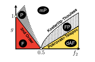
Figure 10: Schematic phase diagram of the $J_{1}$-$J_{2}$QIM: Ferromagnetic (F), dimerized anti-ferromagnetic (dAF), paramagnetic (P), modulated paramagnetic (mP), and floating (FP) phases. These states of matter are separated by different types of quantum phase transitions (Second Order, Kosterlitz-Thouless, and Pokrovsky-Talapov), and by the disorder line (dashed line).

We are interested on the impact that quantum fluctuations may have on these degeneracies. For $g\gg 1\gg f_{2}$, the ground state corresponds to a single paramagnetic (P) state with all spins pointing towards the direction of the transverse field

$$|{\rm P}\rangle=\left|{}_{\rightarrow}{}^{\rightarrow}_{\rightarrow}\cdots_{\rightarrow}{}^{\rightarrow}_{\rightarrow}\right\rangle,$$ (46)

where $|{\rightarrow}\rangle=(|{\uparrow}\rangle+|{\downarrow}\rangle)/\sqrt{2}$. The situation gets more interesting for intermediate fields, whereby additional exotic phases and a variety of quantum phase transitions occur. Since the model is no longer integrable, the analysis of the full phase diagram has been a big challenge, requiring the combination of a variety of techniques. For instance, the mapping to a classical 2D model annni_hamiltonian yields a direct link to commensurate-incommensurate thermal phase transitions classical_annni_review ; annni_comensurability . Hence, it is possible to use the methods developed in this area in order to understand the magnetic phases of the quantum model, being numerical Monte Carlo annni_montecarlo and free-fermion approximations annni_fermionization two representative examples. Together with the more recent application of bosonization techniques allen_bosonization and numerical renormalization group methods anni_dmrg , these studies yield the rich phase diagram represented in Fig. 10. Note that in addition to the aforementioned phases, there is a modulated paramagnetic phase (mP), and a highly-debated incommensurate floating phase (FP). Since all these different phases meet at $f_{\rm c}=\textstyle\frac{1}{2}$, this macroscopically-degenerate point is also known as the multi-phase point. There are several critical lines emerging from the multi-phase point, which give rise to quantum phase transitions of second order, Kosterlitz-Thouless kt_transition , or Pokrovski-Talapov pt_transition type.

Notwithstanding these big efforts, we emphasize that there still exists some controversy about the floating phase. In particular, the extent of the floating phase is still a question of debate. Whereas some results point towards a FP that prolongs towards $f_{2}\gg 1$, other treatments predict a finite region that terminates in a multi-critical Lifshitz point (see itf_glass and references therein). This makes a QS of the utmost interest to settle down these discrepancies. Moreover, as we discuss in detail below, the introduction of long-range interactions leads to additional open questions that have not been previously addressed to the best of our knowledge. From our numerical survey, we conjecture that the dipolar-range of the couplings leads to the splitting of the multi-phase point and the appearance of an intermediate phase (see Fig. 11).

VI.2 Dipolar-range $J_{1}$-$J_{2}$ quantum Ising model

Trapped ions are an ideal platform to test the effects of long-range Ising interactions. For non-frustrated systems, even if the model belongs to the same universality class as the nearest-neighbor case, these long-range interactions may shift the critical point, and favor long-distance quantum correlations ising_porras . For the frustrated systems under study, the effect of long-range interactions is expected to be more significant.

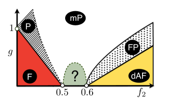
Figure 11: Conjectured phase diagram of the dipolar $J_{1}$-$J_{2}$QIM: The longer-range dipolar Ising couplings, typical of Coulomb-mediated interactions, lead to the splitting of the multiphase point, and the appearance of a different ordered phase in between.

By considering the dipolar range of the trapped-ion ladder Hamiltonian (22), the $J_{1}$-$J_{2}$QIM (43) must be modified to

$$\begin{split}H_{\bigtriangleup\bigtriangledown\bigtriangleup}=-|J_{1}|\bigg{(}&\sum_{i}\sum_{\delta\in{\rm odd}}f_{\delta}\sigma_{i}^{z}\sigma_{i+\delta}^{z}-\\ &-\sum_{i}\sum_{\delta\in{\rm even}}f_{\delta}\sigma_{i}^{z}\sigma_{i+\delta}^{z}+\sum_{i}g\sigma_{i}^{x}\bigg{)},\end{split}$$ (47)

where we have introduced the ratios $f_{\delta}=J_{\delta}/|J_{1}|$, such that $J_{\delta}$ account for the dipolar decay of the interactions. In this notation, the frustration ratio of the nearest-neighbor chain is $f_{2}=J_{2}/|J_{1}|$, and we can study the additional frustration coming from the dipolar range $f_{3},f_{4}...$. We have analyzed numerically the phase diagram of such a long-range frustrated spin model by means of an optimized Lanczos algorithm that allows us to reach efficiently ladders with $L=24$ spins. All the results showed below have been performed including the $f_{3}$ and $f_{4}$ terms of the dipolar tail, in addition to the competing nearest-neighbor ($J_{1}$) and next-to-nearest-neighbor ($J_{2}$) couplings. We have checked that the effect of including longer ranged interactions (i.e., those corresponding to $f_{5}$ and $f_{6}$ couplings) does not affect qualitatively the results.

In order to distinguish the phases, we focus on the two-body correlators, which show the following scaling when $|i-j|\gg 1$

$$\begin{split}&\langle\sigma_{i}^{z}\sigma_{j}^{z}\rangle_{\rm F{\phantom{AF}}}\sim\hskip 4.30554ptm_{0}^{2}\cos(q_{\rm F}(i-j)),\\ &\langle\sigma_{i}^{z}\sigma_{j}^{z}\rangle_{\rm dAF}\sim\hskip 4.30554ptm_{0}^{2}\cos(q_{\rm dAF}(i-j)),\\ &\langle\sigma_{i}^{z}\sigma_{j}^{z}\rangle_{\rm P{\phantom{AF}}}\sim\hskip 4.30554ptm_{0}^{2}\cos(q_{\rm P}(i-j)){\rm e}^{-|i-j|/\xi_{\rm P}},\\ &\langle\sigma_{i}^{z}\sigma_{j}^{z}\rangle_{\rm mP{\phantom{ii}}}\sim\hskip 4.30554ptm_{0}^{2}\cos(q_{\rm mP}(i-j)){\rm e}^{-|i-j|/\xi_{\rm mP}},\\ &\langle\sigma_{i}^{z}\sigma_{j}^{z}\rangle_{\rm FP{\phantom{F}}}\sim\hskip 4.30554ptm_{0}^{2}\cos(q_{\rm FP}(i-j)){|i-j|^{-\eta}},\\ \end{split}$$ (48)

where $0<m_{0}<1$, $\xi_{\rm P},\xi_{\rm mP}$ stand for the correlation lengths of the paramagnets, $\eta>0$ characterizes the algebraic decay of the correlations in the gapless floating phase, and the different modulation parameters $q_{[\dots]}$ have been listed in Table 1.

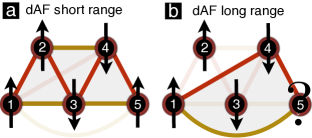
Figure 12: Incompatible sources of partial frustration: (a) The partial frustration for $f_{2}<\textstyle\frac{1}{2}$ in the short-range model can be minimized by one of the four possible dAF ground-states. (b) The introduction of longer-range couplings yields additional sources of frustration, which are incompatible with the dAF ground-state, and thus responsible of the splitting of the multi-phase point.

Table 1: Magnetic modulation parameters

$\hskip 8.61108ptq_{\rm F}\hskip 8.61108pt$	$\hskip 8.61108ptq_{\rm dAF}\hskip 8.61108pt$	$\hskip 8.61108ptq_{\rm P}\hskip 8.61108pt$	$\hskip 8.61108ptq_{\rm mP}\hskip 8.61108pt$	$\hskip 8.61108ptq_{\rm FP}\hskip 8.61108pt$	$\hskip 8.61108ptq_{?}\hskip 8.61108pt$
$0$	$\frac{\pi}{2}$	$0$	$\hskip 8.61108ptq_{\rm mP}(g,f_{2})\hskip 8.61108pt$	$\hskip 8.61108ptq_{\rm FP}(g,f)\hskip 8.61108pt$	?

According to these expressions, the F and d-AF display long-range magnetic order with different periodicities, whereas the P and mP phases are disordered. Finally, the FP phase has quasi-long range order with a modulation parameter that flows with the ratios $f_{2},g$ (hence the adjective floating), and is generally incommensurate with the underlying lattice.

An observable capable of capturing the periodic modulations of the long-range ordered phases, and thus the features of the phase diagram, is the so-called magnetic structure factor. It is defined as the Fourier transform of the spin correlations

$$S_{zz}(q)=\sum_{ij}\langle\sigma_{i}^{z}\sigma_{j}^{z}\rangle{\rm e}^{{\rm i}q(i-j)},$$ (49)

with $q\in[0,2\pi)$, and should attain a maximum at the different values shown in Table 1 for each of the phases. In order to evaluate the magnetic structure factor numerically, we have considered periodic boundary conditions, which shall capture the bulk properties in the center of the trapped-ion ladders.

According to the scheme depicted in fig. 11, the main features of phase diagram of the dipolar $J_{1}$-$J_{2}$QIM can be divided into three different regions: the region where the ferromagnetic order prevails ($f_{2}<0.5$), the region with the dimerized-AF order ($f_{2}>0.6$), and the new intermediate region (roughly, $f_{2}\in(0.5,0.6)$) that appears due to the competition of different long-ranged frustration mechanisms. In Figs. 12(a)-(b), we show how the dAF phase is destabilized by these competing mechanisms, which accounts schematically for the splitting of the multi-phase point. We will show below how the numerical evaluation of the structure factor supports this division. We note that the structure factor has been normalized to unity.

In Fig. 13(a), we plot the order parameter $S_{zz}(\frac{\pi}{2})$ corresponding to the dAF phase. It can be observed that both phase transitions, namely the discontinuous transition (Pokrovski-Talapov type) separating the dAF phase from the FP, and the continuous transition (Kosterlitz-Thouless type) between the FP and the mP phases, reflect themselves clearly in the structure factor as two consecutive jumps with increasing transverse field. The fact that only one transition is observed for lower values of $f_{2}$ hint at the possibility that the multicritical point has been shifted from $g=0$ to some finite value. Whether this shift survives for larger lattices, or corresponds to a finite-size effect, is an open question that cannot be addressed due to the limitations of the diagonalization routine.

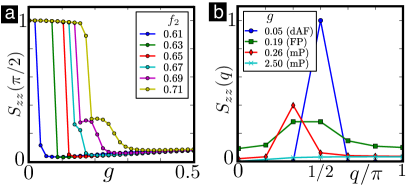
Figure 13: Dipolar $J_{1}$-$J_{2}$QIM (dAF region, L=24): (a) Antiferromagnetic order parameter $S_{zz}(\pi/2)$. (b) Structure factor $S_{zz}(q)$ for $f_{2}=0.69$.

The dependence of the structure factor with the lattice momentum $q$ can be seen in Fig. 13(b). Here, we represent the evolution of this magnitude as we increase $g$ for a fixed value of $f_{2}$. We have chosen some representatives for each phase: for low fields $g$, we are well into the dAF phase, whose periodicity is given by a single $q=\frac{\pi}{2}$ component. Increasing the transverse field $g$, the state undergoes a transition to the FP, showing a ($f_{2}$-, $g$-dependent) incommensurate modulation. Upon further increase of the field, we reach the mP phase. Note that for moderate $g$, the modulation of this phase is apparent in the peaked form of its structure factor. Increasing further the magnetic field polarizes the spins in the transversal direction yielding a flat vanishing structure factor.

The same analysis has been carried out in the ferromagnetic region. In Fig. 14(a), we have plotted the $S_{zz}(0)$ component characteristic of a ferromagnet. In this case, however, only one clear phase transition arises as we increase the transverse field $g$ for a fixed value of $f_{2}$. Also in accordance with this observation, the modulation of the ground-state in Fig. 14(b), shows a shift between a pure ferromagnetic order for low values of $g$, to a modulated paramagnetic one with increasing field, and finally to the completely polarized paramagnet for $g\gg 1$. This suggests the possibility that the unmodulated paramagnetic phase observed in the $J_{1}$-$J_{2}$QIM is not stable upon the effect of further dipolar couplings, or that its extent in the phase diagram is small enough to prevent to be accurately captured with finite-sized lattices.

In the $J_{1}$-$J_{2}$QIM, there exists a one-point boundary between the ferromagnetic and dimerized-antiferromagnetic phases precisely located at the muticritical point $(g=0,f_{2}=0.5)$. Interestingly enough, in the dipolar $J_{1}$-$J_{2}$QIM this is no longer true and both phases are separated by a finite region. In Fig. 15(a), we have plotted the structure factor $S_{zz}(q)$ for the lattice size $L=16$ along a fixed value of $f_{2}$ in between the F- and dAF-phases. In this graph, a new type of modulation shows up in the form of two diferentiated peaks with momenta $q_{1}=\frac{\pi}{4}$ and $q_{2}=\frac{3\pi}{4}$. However, the precision in the determination of such peaks is limited by the size of our lattice. We have carried out additional numerics for $L=24$, which allow us to bound these peaks between $q_{1}\in[\frac{\pi}{6},\frac{\pi}{3}]$ and $q_{2}\in[\frac{2\pi}{3},\pi]$. We have checked that the relative amplitude of these peaks does not depend on the ratio between the intra- and inter-leg couplings. In Fig. 15(b), we plot the amplitude of these two characteristic peaks with increasing $g$. The shaded area represents the range where both peaks coexist, i.e, the extent of the new ordered state. It would be very interesting to explore the precise origin of these modulations via the trapped-ion QS.

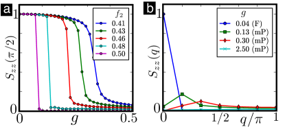
Figure 14: Dipolar $J_{1}$-$J_{2}$QIM (F region, L=24): (a) Ferromagnetic order parameter $S_{zz}(0)$. (b) Structure factor $S_{zz}(q)$ for $f_{2}=0.45$

We remark that the modulations $q_{1}$ and $q_{2}$ coexist for low transverse fields. As we increase $g$, only the modulation with lower lattice momentum survives as a differentiated peak. Indeed, the momentum of this surviving modulation is compatible with that found in the mP phase for intermediate fields (compare the light-blue curve in Fig. 15(a) with the red ones in Figs. 14(b) and 13(b)). Whether this is a crossover or a quantum phase transition between the new conjectured phase and the mP, goes beyond the limitations of our numerical tools.

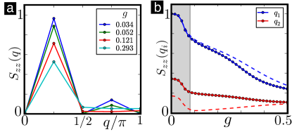
Figure 15: Dipolar $J_{1}$-$J_{2}$QIM (intermediate region): (a) Structure factor computed in a lattice of size $L=16$. (b) Amplitude of the two differentiated peaks in the intermediate region. The accuracy of its location is conditioned by the size of the lattice: (solid lines) $L=24$, $q_{1}=\frac{\pi}{3}$ and $q_{2}=\frac{5\pi}{3}$ (dashed lines) $L=16$, $q_{1}=\frac{\pi}{4}$, $q_{2}=\frac{3\pi}{4}$.

All the above results have been computed in ladders

$$\tilde{x}_{i}^{0}=\frac{d}{2}(-1)^{i},\hskip 4.30554pt\tilde{y}_{i}^{0}=0,\hskip 4.30554pt\tilde{z}_{i}^{0}=(i-\textstyle\frac{1}{2}N)a,$$ (50)

with lattice parameters $d=a$ . Note that a ladder composed of equilateral triangles would correspond to $d=\sqrt{3}a$. The extent of the new intermediate phase in the dipolar $J_{1}$-$J_{2}$QIM is indeed strongly dependent on the geometry of the triangular plaquettes. A straightforward way of measuring the extent of this phase is computing the distance between the F and dAF phases along the line $g=0$. In Fig. 16, we show the order parameters $S_{zz}(0)$, $S_{zz}(\pi/4)$ and $S_{zz}(\pi/2)$ for different values of the anisotropy ratio $d/a$, which correspond to the F phase, the new intermediate phase, and the dAF phase, respectively. From these graphs (qualitatively similar results are obtained with $L=24$), it is apparent that the splitting of the multiphase point is strongly enhanced in anisotropic lattices.

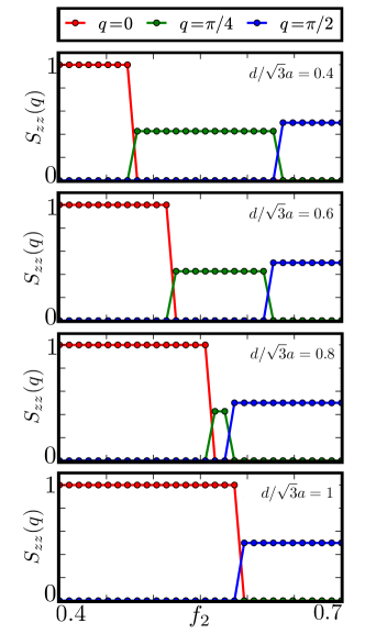
Figure 16: Splitting of the multiphase critical point: order parameters corresponding to the F ($S_{zz}(0)$) intermediate ($S_{zz}(\pi/4)$)and dAF ($S_{zz}(\pi/2)$) phases computed in a $L=16$ lattice. Each figure corresponds to a fixed anisotropy ratio $d/a$. The homogeneous equilateral zigzag lattice corresponds to $d/a=\sqrt{3}$ (figure at the bottom).

VII Conclusions and Outlook

Low-dimensional quantum Ising magnets are often representative models for a variety of emergent cooperative phenomena. Unfortunately, in contrast to their Heisenberg counterparts, the identification of materials accurately described by these models has turned out to be a much more difficult task. Moreover, whenever the models include anisotropic interactions and tunable ladder structures, the prospects of realizing them diminish even further. A promising alternative to overcome such difficulties are the so-called quantum simulators.

In this work, we have shown that cold ion crystals are promising candidates for the quantum simulation of a variety of quantum spin-ladder compounds. This avenue of research will allow for the study of collective phenomena due to the combination of frustration, quantum fluctuations, long-range interactions, and dimensional crossover. In particular, these ion crystals can be used to explore paradigmatic, yet controversial, models of quantum Ising ladders whereby analytical and numerical techniques seem to disagree. Moreover, they may also allow for the study of previously unexplored features of the models, such as the effects of long-range interactions.

First, we have shown how to control the geometry of different self-assembled trapped-ion ladders. Based on this possibility, we have presented a protocol to tailor the anisotropy of the magnetic interaction mediated by the transverse phonons, which couple pairs of distant ions indirectly. When these ions belong to different legs of the ladder, it is possible to tune both the sign and the magnitude of the spin-spin couplings by manipulating the laser-beam arrangement. The validity of this technique is supported by a detailed discussion of the possible sources of error in current ion-trap experiments, and by numerics showing an excellent agreement with our predictions.

This tool opens a vast amount of possibilities for trapped-ion-based QS of cooperative magnetic phenomena. For instance, we have presented a thorough description of the QS for the cornerstone of frustrated quantum Ising magnets, the $J_{1}$-$J_{2}$ quantum Ising model. Moreover, we have also discussed how the QS has the potential of realizing quantum Ising ladders with connections to the exotic quantum dimer models introduced in the context of high-temperature superconductivity, and address the intriguing dimensional crossover phenomena. Finally, we have also pointed out how this QS may yield a route towards the long-sought quantum spin liquid phases.

Appendix A Spin-dependent dipole forces and dissipation

In this Appendix, we present a detailed derivation of the effective laser-ion interaction sd_force ; sd_force_review in Eq. (10). By taking into account the spontaneous decay from the excited level (see Fig. 3), we can discuss the regime where the spin-dependent dipole forces arise, and also analyze the sources of error due to photon scattering in the experiments. We consider the master equation for the Lambda scheme in Fig. 3, namely

$$\frac{{\rm d}\rho}{{\rm d}t}=-{\rm i}[H_{0}+V,\rho(t)]+\mathcal{D}(\rho(t)).$$ (51)

The coherent part of the evolution is given by

$$H_{0}=\!\!\!\!\sum_{m=r,\uparrow,\downarrow}\!\!\!\!\!\epsilon_{m}|m\rangle\langle m|,\hskip 4.30554ptV=\!\!\!\sum_{l=1,2}\sum_{s=\uparrow,\downarrow}\!\textstyle\frac{1}{2}\Omega_{l,s}|r\rangle\langle s|{\rm e}^{-{\rm i}\omega_{l}t}+\text{H.c.},$$ (52)

where we have introduced the energies of the internal states $\epsilon_{r},\epsilon_{\uparrow},\epsilon_{\downarrow}$, the Rabi frequencies of the transitions $\Omega_{l,s}$, and the laser frequencies $\omega_{l}$. The dissipator describing the spontaneous decay from the excited state is of the Lindblad form

$$\mathcal{D}(\rho)=\sum_{n=1,2}\left(L_{n}\rho L_{n}^{\dagger}-\textstyle\frac{1}{2}L_{n}^{\dagger}L_{n}\rho-\textstyle\frac{1}{2}\rho L_{n}^{\dagger}L_{n}\right),$$ (53)

with the following jump operators $L_{1}=\sqrt{\Gamma}|{\downarrow}\rangle\langle r|$, and $L_{2}=\sqrt{\Gamma}|{\uparrow}\rangle\langle r|$, where $\Gamma$ is the spontaneous decay rate from the excited state back to the spin manifold (see Fig. 3). Let us now define the detunings for all possible transitions

$$\delta_{l,s}=\epsilon_{r}-\epsilon_{s}-\omega_{l}.$$ (54)

As announced in the main text, when these detunings are much larger than the Rabi frequencies and the decay rate, namely $\delta_{l,s}\gg\Omega_{l,s},\Gamma$, it is possible to adiabatically eliminate the excited state from the dynamics, and obtain an effective master equation within the spin manifold. We use the formalism introduced in eff_jumps , and obtain the master equation

$$\begin{split}\frac{{\rm d}\rho}{{\rm d}t}&=-{\rm i}[H_{\rm eff},\rho(t)]+\\ &+\sum_{n}\left(L^{\rm eff}_{n}\rho(L^{\rm eff}_{n})^{\dagger}-\textstyle\frac{1}{2}(L^{\rm eff}_{n})^{\dagger}L^{\rm eff}_{n}\rho-\textstyle\frac{1}{2}\rho(L^{\rm eff}_{n})^{\dagger}L^{\rm eff}_{n}\right),\end{split}$$ (55)

where the Hamiltonian is $H_{\rm eff}=H_{\rm s}+H_{\rm r}+H_{\rm d}$, such that

$$H_{\rm s}=(\epsilon_{\downarrow}+\Delta\epsilon_{\downarrow})|{\downarrow}\rangle\langle{\downarrow}|+(\epsilon_{\uparrow}+\Delta\epsilon_{\uparrow})|{\uparrow}\rangle\langle{\uparrow}|$$ (56)

includes the following ac-Stark shifts

$$\Delta\epsilon_{s}=-\sum_{l=1,2}\frac{|\Omega_{l,s}|^{2}\delta_{l,s}}{4\delta_{l,s}^{2}+\Gamma_{\rm t}^{2}},$$ (57)

and we have introduced the sum of the two decay rates $\Gamma_{\rm t}=2\Gamma$. Additionally, we get the following two-photon stimulated Raman transitions

$$H_{\rm r}=\sum_{l,l^{\prime}}\textstyle\frac{1}{2}\Omega^{\rm r}_{l,l^{\prime}}\sigma^{-}{\rm e}^{{\rm i}(\omega_{l}-\omega_{l^{\prime}})t}+{\rm H.c.},$$ (58)

where we have introduced $\sigma^{-}=|{\downarrow}\rangle\langle{\uparrow}|=(\sigma^{+})^{\dagger}$, and the effective Rabi frequencies for the different Raman transitions

$$\Omega^{\rm r}_{l,l^{\prime}}=-\frac{\Omega_{l,\downarrow}^{*}\Omega_{l^{\prime},\uparrow}(\delta_{l,\downarrow}+\delta_{l^{\prime},\uparrow})}{(2\delta_{l,\downarrow}+{\rm i}\Gamma_{\rm t})(2\delta_{l^{\prime},\uparrow}-{\rm i}\Gamma_{\rm t})},$$ (59)

which involve the absorption of a photon from the beam $l^{\prime}=1,2$ and posterior photon emission into the beam $l=1,2$. The last term of the effective Hamiltonian is the one responsible for the spin-dependent dipole forces

$$H_{\rm d}=\sum_{s=\uparrow,\downarrow}\textstyle\frac{1}{2}\Omega^{\rm d}_{s}|s\rangle\langle s|{\rm e}^{{\rm i}(\omega_{1}-\omega_{2})t}+\text{H.c.},$$ (60)

where we have introduced the following Rabi frequencies

$$\Omega^{\rm d}_{s}=-\frac{\Omega_{1,s}^{*}\Omega_{2,s}(\delta_{1,s}+\delta_{2,s})}{(2\delta_{1,s}+{\rm i}\Gamma_{\rm t})(2\delta_{2,s}-{\rm i}\Gamma_{\rm t})}.$$ (61)

Now, depending on the particular laser frequencies $\omega_{l}$, it is possible to select whether the laser-ion interaction leads to a stimulated Raman transition (i.e. $\omega_{\rm L}:=\omega_{1}-\omega_{2}\approx\epsilon_{\uparrow}-\epsilon_{\downarrow}=:\omega_{0}$), or to a spin-dependent dipole force (i.e. $\omega_{\rm L}\ll\omega_{0}$). The effects of the spin-dependent dipole force are more transparent by rewriting Eq. (60) as follows

$$H_{\rm d}=\textstyle\frac{1}{2}\tilde{\Omega}_{\rm L}\mathbb{I}{\rm e}^{-{\rm i}\omega_{\rm L}t}+\textstyle\frac{1}{2}{\Omega}_{\rm L}\sigma^{z}{\rm e}^{-{\rm i}\omega_{\rm L}t}+\text{H.c.},$$ (62)

where we have introduced $\sigma^{z}=|{\uparrow}\rangle\langle{\uparrow}|-|{\downarrow}\rangle\langle{\downarrow}|$, and

$$\tilde{\Omega}_{\rm L}=\textstyle\frac{1}{2}\big{(}\Omega^{\rm d}_{\uparrow}+\Omega^{\rm d}_{\downarrow}\big{)}^{*},\hskip 4.30554pt{\Omega}_{\rm L}=\textstyle\frac{1}{2}\big{(}\Omega^{\rm d}_{\uparrow}-\Omega^{\rm d}_{\downarrow}\big{)}^{*}.$$ (63)

Once the coherent part of the effective master equation has been derived, one must obtain the effective jump operators. In our setup, they can be expressed as follows

$$\begin{split}L_{1}^{\rm eff}&=\sqrt{\Gamma}\left(\frac{\Omega_{1,\downarrow}{\rm e}^{-{\rm i}\omega_{1}t}}{\delta_{1,\downarrow}-{\rm i}\Gamma_{\rm t}}+\frac{\Omega_{2,\downarrow}{\rm e}^{-{\rm i}\omega_{2}t}}{\delta_{2,\downarrow}-{\rm i}\Gamma_{\rm t}}\right)|{\downarrow}\rangle\langle{\downarrow}|+\\ &+\sqrt{\Gamma}\left(\frac{\Omega_{1,\uparrow}{\rm e}^{-{\rm i}\omega_{1}t}}{\delta_{1,\uparrow}-{\rm i}\Gamma_{\rm t}}+\frac{\Omega_{2,\uparrow}{\rm e}^{-{\rm i}\omega_{2}t}}{\delta_{2,\uparrow}-{\rm i}\Gamma_{\rm t}}\right)|{\downarrow}\rangle\langle{\uparrow}|,\\ L_{2}^{\rm eff}&=\sqrt{\Gamma}\left(\frac{\Omega_{1,\uparrow}{\rm e}^{-{\rm i}\omega_{1}t}}{\delta_{1,\uparrow}-{\rm i}\Gamma_{\rm t}}+\frac{\Omega_{2,\uparrow}{\rm e}^{-{\rm i}\omega_{2}t}}{\delta_{2,\uparrow}-{\rm i}\Gamma_{\rm t}}\right)|{\uparrow}\rangle\langle{\uparrow}|+\\ &+\sqrt{\Gamma}\left(\frac{\Omega_{1,\downarrow}{\rm e}^{-{\rm i}\omega_{1}t}}{\delta_{1,\downarrow}-{\rm i}\Gamma_{\rm t}}+\frac{\Omega_{2,\downarrow}{\rm e}^{-{\rm i}\omega_{2}t}}{\delta_{2,\downarrow}-{\rm i}\Gamma_{\rm t}}\right)|{\uparrow}\rangle\langle{\downarrow}|.\\ \end{split}$$ (64)

Note that the first term of each of the effective jump operators corresponds to the so-called Rayleigh photon scattering, which takes place without modifying the internal spin state. In this formulation, it becomes clear why the Rayleigh scattering will only introduce dephasing when the amplitudes (i.e. terms between brackets) of each jump operator are different, as observed in recent experiments photon_scattering_2 . The second term of each jump operator corresponds to the Raman scattering, whereby the spin state is changed after the emission of the photon.

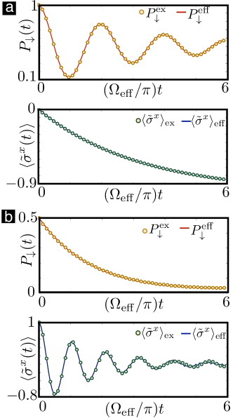
Figure 17: Effective dissipative dynamics: (a) Population $P_{\downarrow}(t)={\rm Tr}\big{\{}|{\downarrow}\rangle\langle{\downarrow}|\rho(t)\big{\}}$, and coherences $\langle\tilde{\sigma}^{x}\rangle={\rm Tr}\big{\{}|{\downarrow}\rangle\langle{\uparrow}|{\rm e}^{-{\rm i}\omega_{0}t}\rho(t)\big{\}}+\text{c.c.}$ in the regime of two-photon stimulated Raman transitions. (b) Same observables in the regime of spin-dependent dipole forces.

In order to study the accuracy of this effective description (55), we confront it with the exact numerical integration of the original master equation (51). In Fig. 17(a), we compare both predictions for $\epsilon_{\uparrow}/\epsilon_{r}=0.1,\epsilon_{\downarrow}/\epsilon_{r}=0.05$, and setting the laser parameters such that $\delta_{1,\uparrow}/\epsilon_{r}=0.5$, $\omega_{\rm L}=\omega_{0}$, $\Omega_{2,\uparrow}/\epsilon_{r}=\Omega_{1,\downarrow}/\epsilon_{r}=0.05$, and $\Omega_{1,\uparrow}=\Omega_{2,\downarrow}=0$. This set of parameters leads to the regime of stimulated two-photon transitions, so that we expect to find periodic Rabi oscillations in the populations with a frequency $\Omega_{\rm eff}/\epsilon_{r}=2.5\cdot 10^{-3}$ when the initial state is $|\psi_{0}\rangle=|{\downarrow}\rangle$. As shown in the upper panel of Fig. 17(a), these oscillations get damped due to the spontaneous decay $\Gamma/\epsilon_{r}=0.05$, where a clear agreement of the exact and effective dynamics can be observed. In the lower panel, we represent the time-evolution of the coherences, which are damped due to the photon scattering.

More interesting to our purposes are the results displayed in Fig. 17(b), where we have kept the same parameters as above, but set $\omega_{\rm L}=10^{-3}\omega_{0}$. This guarantees the absence of two-photon Raman transitions. By switching on the additional laser beams, such that $\Omega_{2\downarrow}/\epsilon_{r}=-\Omega_{1\uparrow}/\epsilon_{r}=0.05$, the non-vanishing differential Rabi frequency in Eq. (63) should lead to the $\sigma^{z}$ dipole force (62). Accordingly, we expect to find damped Rabi oscillations in the coherences for $|\psi_{0}\rangle=(|\uparrow\rangle+|\downarrow\rangle)/\sqrt{2}$, whereas the populations should only show an exponential damping. This agrees with the results displayed in Fig. 17(b), which also support the accuracy of the effective master equation in this regime.

To recover the action of the lasers on the vibrational degrees of freedom, one should substitute $\Omega_{l,s}\to\Omega_{l,s}{\rm e}^{{\rm i}{\bf k}_{l}\cdot{\bf r}}$ in all the expressions above. Besides, in the regime of interest

$$|\Omega^{\rm r}_{l,l^{\prime}}|\ll\omega_{0}\ll\epsilon_{r}-\epsilon_{\uparrow},\hskip 4.30554pt{\rm and}\hskip 4.30554pt\Gamma_{\rm t}\ll\delta_{l,s}\approx\delta_{1,\uparrow}=:\Delta,$$ (65)

and summing over all the trapped ions, one recovers the dipole force term in Eq. (10) with the effective Rabi frequency $\Omega_{\rm L}=\frac{1}{2\Delta}\big{(}\Omega_{1,\downarrow}\Omega_{2,\downarrow}^{*}-\Omega_{1,\uparrow}\Omega_{2,\uparrow}^{*}\big{)}$. Let us note that the running wave of strength $\tilde{\Omega}_{\rm L}$ that only couples to the vibrational excitations, together with the ac-Stark shifts contained in (57), must be compensated experimentally. Finally, the expression for the effective jump operators is the following

$$\begin{split}L_{1}^{\rm eff}&=\frac{\sqrt{\Gamma}}{\Delta}\left(\Omega_{1,\downarrow}{\rm e}^{{\rm i}({\bf k}_{1}\cdot{\bf r}-\omega_{1}t)}+\Omega_{2,\downarrow}{\rm e}^{{\rm i}({\bf k}_{2}\cdot{\bf r}-\omega_{2}t)}\right)|{\downarrow}\rangle\langle{\downarrow}|+\\ &+\frac{\sqrt{\Gamma}}{\Delta}\left(\Omega_{1,\uparrow}{\rm e}^{{\rm i}({\bf k}_{1}\cdot{\bf r}-\omega_{1}t)}+\Omega_{2,\uparrow}{\rm e}^{{\rm i}({\bf k}_{2}\cdot{\bf r}-\omega_{2}t)}\right)|{\downarrow}\rangle\langle{\uparrow}|,\\ L_{2}^{\rm eff}&=\frac{\sqrt{\Gamma}}{\Delta}\left(\Omega_{1,\uparrow}{\rm e}^{{\rm i}({\bf k}_{1}\cdot{\bf r}-\omega_{1}t)}+\Omega_{2,\uparrow}{\rm e}^{{\rm i}({\bf k}_{2}\cdot{\bf r}-\omega_{2}t)}\right)|{\uparrow}\rangle\langle{\uparrow}|+\\ &+\frac{\sqrt{\Gamma}}{\Delta}\left(\Omega_{1,\downarrow}{\rm e}^{{\rm i}({\bf k}_{1}\cdot{\bf r}-\omega_{1}t)}+\Omega_{2,\downarrow}{\rm e}^{{\rm i}({\bf k}_{2}\cdot{\bf r}-\omega_{2}t)}\right)|{\uparrow}\rangle\langle{\downarrow}|.\\ \end{split}$$ (66)

Since we are considering that $|\Omega_{l,s}|\ll\Delta$, it becomes clear that the effective scattering rates scale as $\Gamma_{\rm eff}=\Gamma(|\Omega_{l,s}|/\Delta)^{2}$.

Appendix B Analysis of the ion micromotion

In this Appendix, we take into account the micromotion by considering the radio-frequency (r.f.) trapping fields rather than the effective pseudo-potential in Eq. (1) ion_trap_book . More precisely, the trapping potential is

$$\begin{split}V_{\rm t}(\{{\bf r}_{j}\})=&-\frac{e}{2}V_{0}\cos(\Omega_{\rm rf}t)\sum_{i}\left(1+\frac{1}{r_{0}^{2}}\left(x_{i}^{2}-y_{i}^{2}\right)\right)\\ &-e\kappa_{\rm g}U_{0}\sum_{i}\frac{1}{z_{0}^{2}}\left(z_{i}^{2}+\frac{1}{2}\left(x_{i}^{2}+y_{i}^{2}\right)\right),\end{split}$$ (67)

where $V_{0},U_{0}$ are the a.c. and d.c. potentials of the trap, $r_{0},z_{0}$ are the distances from the trap center to the electrodes and end-caps respectively, and $\kappa_{\rm g}<1$ is a geometric factor. Together with the Coulomb interaction, this trapping potential leads to a set of coupled Mathieu equations

$$\frac{{\rm d}^{2}r_{i\alpha}}{{\rm d}t^{2}}+\frac{\Omega_{\rm rf}^{2}}{4}[a_{\alpha}+2q_{\alpha}\cos(\Omega_{\rm rf}t)]r_{i\alpha}-\frac{e^{2}}{m}\sum_{j\neq i}\frac{r_{i\alpha}-r_{j\alpha}^{\phantom{3/3}}}{|{\bf r}_{i}-{\bf r}_{j}|^{3}}=0,$$ (68)

where we have defined $a_{x}=4e\kappa_{\rm g}U_{0}/mz_{0}^{2}\Omega_{\rm rf}^{2}=a_{y}=-a_{z}/2$, and $q_{x}=-2eV_{0}/mr_{0}^{2}\Omega_{\rm rf}^{2}=-q_{y},q_{z}=0$. In the majority of the experimental setups, these parameters fulfill $a_{\alpha},q_{\alpha}^{2}\ll 1$, so that one finds the following solution

$$r_{i\alpha}=r_{i\alpha}^{0}\left(1+\textstyle\frac{1}{2}q_{\alpha}\cos(\Omega_{\rm rf}t)\right)+\Delta r_{i\alpha}(t)$$ (69)

where $\Delta{\bf r}_{i}(t)$ stand for the secular vibrations of the ions and frequency shifts due to micromotion Ferdiand_exp ; Landa_micromotion that shall lead to the phonon Hamiltonian (9), and ${\bf r}_{i}^{0}$ are the equilibrium positions of the ion crystal. To lowest order in $a_{\alpha},q_{\alpha}^{2}$, these are found from the static part of Eq. (68), after solving

$$\frac{m}{4}\Omega_{\rm rf}^{2}\left(a_{\alpha}+\frac{1}{2}q_{\alpha}^{2}\right)r_{i\alpha}^{0}-e^{2}\sum_{i\neq j}\frac{r^{0}_{i\alpha}-r^{0}_{j\alpha}}{|{{\bf r}^{0}_{i}-{\bf r}^{0}_{j}|^{3}}}=0,$$ (70)

which is equivalent to Eq. (2) after identifying the effective trapping frequencies $\omega_{\alpha}=\textstyle\frac{1}{2}\Omega_{\rm rf}(a_{\alpha}+\textstyle\frac{1}{2}q_{\alpha}^{2})^{1/2}$. From Eq. (69), one identifies two sources of radial micromotion. The second term corresponds to the micromotion associated to the small-amplitude secular vibrations of the ions, whereas the first term stands for an additional micromotion connected to the equilibrium positions lying off the trap axis. The former can be minimized by laser cooling, whereas the latter is a driven motion that cannot be cooled, and is intrinsically linked to the planar structure of the ladder geometries (i.e. for linear ion chains, this micromotion can be compensated by aligning the ions along the trap axis). Let us remark that for the regimes of interest, $q_{x}\approx 0.1$-$0.2$, $l_{z}\approx 1$-$10$ $\mu$m, this micromotion can largely exceed that created by the secular oscillations, and must be thus considered as a potential source of error in our QS. The discussion below focuses on this type of micromotion $r_{i\alpha}^{0}(t)=r_{i\alpha}^{0}\left(1+\textstyle\frac{1}{2}q_{\alpha}\cos(\Omega_{\rm rf}t)\right)$, which is usually referred to as the excess micromotion micromotion_wineland .

Micromotion heating: One possible consequence of the micromotion is undesired heating, either due to the r.f. field of the ion trap, or to the additional lasers used for cooling. In particular, we focus on the transverse phonons since they are responsible for the spin-spin interaction.

One term in the effect of micromotion can be understood from the interplay between the excess micromotion and those terms in the vibrational Hamiltonian (3) that do not conserve the number of vibrational excitations. By working in the local vibrational basis used in Sec. III, these terms amount to

$$\Delta H(t)=\frac{\omega_{z}}{2}\sum_{i,j}\kappa_{y}^{1/2}\mathcal{\tilde{V}}_{ij}^{yy}(t)a_{i,y}^{\dagger}a_{j,y}^{\dagger}{\rm e}^{2{\rm i}\omega_{y}t}+{\rm H.c.},$$ (71)

where the couplings $\mathcal{\tilde{V}}_{ij}^{yy}(t)=\mathcal{{V}}_{ij}^{yy}(t)/(e^{2}/l_{z}^{3})$ correspond to those of Eq. (4) after taking into account the micromotion

$$r_{i\alpha}^{0}\to r_{i\alpha}^{0}(t)=r_{i\alpha}^{0}\left(1+\textstyle\frac{1}{2}q_{\alpha}\cos(\Omega_{\rm rf}t)\right).$$ (72)

In order to neglect $\Delta H(t)$, which is responsible of the r.f. heating, we expand Eq. (71) to leading order in $q_{\alpha}\ll 1$, and find that all the relevant terms can be neglected under a RWA if the following condition is fulfilled

$$\kappa_{y}^{1/2}|\mathcal{\tilde{V}}^{yy}_{ij}|\ll\frac{|2\omega_{y}\pm\Omega_{\rm rf}|}{\omega_{z}}\approx\frac{\Omega_{\rm rf}}{\omega_{z}}.$$ (73)

Since the ladder compounds present $\kappa_{y}\ll 1$, and $\Omega_{\rm rf}\gg\omega_{z}$, the validity of the RWA is easily fulfilled. Thus the leading r.f. heating mechanism would be due to non linearities. This mechanism was analysed numerically in Schuessler_Heating ; Drewsen_Heating , where scaling laws for the r.f. heating rates were predicted. In these studies, the heating rates originate from non linearities and thus scale with the initial temperature of the crystal. For the temperatures that apply for our scheme, the r.f. heating would be much smaller than the anomalous heating and thus could be neglected in our analysis.

A different possibility is that of laser heating. Note that the QS requires laser cooling of the transverse phonon modes, although not necessarily to the ground-state. As emphasized in laser_micromotion_heating ; micromotion_wineland , depending on the ratio of the r.f. frequency to the decay rate of the cooling transition, either a broadening of the transition or the appearance of multiple micromotion sidebands may occur, which can lead to undesired heating even when the laser frequency is tuned below the atomic resonance. To overcome this effect, one must carefully tune the laser frequency according to the regimes described in micromotion_wineland .

Micromotion contribution to the spin-dependent forces: An important question to address is whether the micromotion modifies the spin-dependent dipole force, as derived in Appendix A. In the interaction picture, the Hamiltonian describing the laser coupling (52) for the whole ion crystal becomes

$$V(t)=\sum_{l,s}\sum_{i}\frac{1}{2}\Omega_{l,s}|r_{i}\rangle\langle s_{i}|{\rm e}^{{\rm i}{\bf k}_{l}\cdot{\bf r}_{i}}{\rm e}^{{\rm i}\xi_{li}\cos(\Omega_{\rm rf}t)}{\rm e}^{{\rm i}\delta_{l,s}t}+\text{H.c.},$$ (74)

after including the micromotion. Here, we have introduced $\xi_{li}=q_{x}{\bf k}_{l}\cdot{\bf r}_{i}^{0}/2$, which represents the ratio of the radial excess micromotion (69) to the wavelength of the laser radiation.

To carry on with the analysis, we need to specify a particular laser-beam arrangement (see the inset of Fig. 2(b)). We parametrize the laser wavevectors as follows

$${\bf k}_{l}=\frac{2\pi}{\lambda_{\rm sp}}(\cos\alpha_{l}{\bf e}_{x}+\sin\alpha_{l}{\bf e}_{y}),$$ (75)

where $\alpha_{l}$ determines their angle with respect to the $x$-axis, and $\lambda_{\rm sp}$ is the wavelength of the $n^{2}S_{1/2}$-$n^{2}P_{3/2}$ transition (see Fig. 3). Let us recall that in order to control the anisotropy of the spin interactions (19), $\tilde{J}^{\rm eff}_{ij}\propto\cos(\phi_{ij})$, the corresponding angles must span the range $\phi_{ij}\in[0,2\pi]$. This implies that the laser-beam arrangement must fulfill $\alpha_{1}=-\alpha_{2}-\Delta\alpha$, where $\Delta\alpha\ll|\alpha_{l}|$. One particular choice is the following

$$\alpha_{2}=\frac{\pi}{2},\hskip 4.30554pt\alpha_{1}=-\frac{\pi}{2}-\Delta\alpha,\hskip 12.91663pt\Delta\alpha\approx\frac{\lambda_{\rm sp}}{2d}\ll 1,$$ (76)

where $d$ is the inter-leg distance (see Fig. 4). With this choice, we find $\xi_{2i}=0$, and $\xi_{1i}=\pm\frac{\pi}{4}q_{x}$, both fulfilling $|\xi_{li}|\ll 1$. This property will allow us to truncate the following series

$${\rm e}^{{\rm i}\xi_{li}\cos(\Omega_{\rm rf}t)}=\sum_{m\in\mathbb{Z}}{\rm i}^{m}J_{m}(\xi_{li}){\rm e}^{{\rm i}m\Omega_{\rm rf}t},$$ (77)

where $J_{m}(x)$ are the Bessel functions of the first kind. By substituting the series (77) in the laser-ion coupling (74), we obtain a sum over all possible micromotion sidebands

$$V(t)\propto\sum_{l,s,i}\sum_{m}\frac{1}{2}\Omega_{l,s}J_{m}(\xi_{li})|r_{i}\rangle\langle s_{i}|{\rm e}^{{\rm i}{\bf k}_{l}\cdot{\bf r}_{i}}{\rm e}^{{\rm i}(\delta_{l,s}-m\Omega_{\rm rf})t}+\text{H.c.}.$$ (78)

According to Eq. (65), we can set $\Delta\approx\delta_{l,s}$, such that for a sufficiently large detuning $\Omega_{\rm rf}/2\pi\approx 0.1$ GHz $\ll\Delta/2\pi\approx 10$ GHz, we find that the micromotion sidebands only introduce a resonance for $m\approx 10$. However, the contribution of such terms is negligible since $\xi_{li}\ll 1$, and $J_{m}(\xi_{li})\propto(\xi_{li})^{m}$. As shown in Wineland_micromotion , the correction to the leading term should be taken into account by adjusting the Rabi frequency. Let us also note that the remaining non-resonant sidebands can also be neglected in a RWA, since $|\Omega_{l,s}|\ll\Delta$. Hence, we conclude that the validity of the spin-dependent dipole force derived in Appendix A is not compromised by the micromotion.

To quantify the accuracy of this argument, we introduce

$$\epsilon_{{\rm m}}={\rm max}_{t}\left\{\big{|}\langle\tilde{\sigma}^{x}(t)\rangle_{\rm mic}-\langle\tilde{\sigma}^{x}(t)\rangle_{\rm eff}\big{|},\hskip 2.15277ptt\in\left[0,\textstyle{\frac{6\pi}{\Omega_{\rm L}}}\right]\right\},$$ (79)

where $\langle\tilde{\sigma}^{x}(t)\rangle={\rm Tr}\big{\{}|{\downarrow}\rangle\langle{\uparrow}|{\rm e}^{-{\rm i}\omega_{0}t}\rho(t)\big{\}}+\text{c.c.}$ represents the coherences. In this expression, the effective evolution under the dipole force $\langle\tilde{\sigma}^{x}(t)\rangle_{\rm eff}$, as represented in Fig. 17(b), is compared to the time evolution including the micromotion sidebands $\langle\tilde{\sigma}^{x}(t)\rangle_{\rm mic}$. Accordingly, $\epsilon_{{\rm m}}$ sets an upper bound to the error of the dipole force (10). In Fig. 18, we represent this error bound as a function of the relative micromotion amplitude $\xi_{1i}$. We use the same parameters as in Appendix A, and set the r.f. frequency to $\Omega_{\rm rf}/\epsilon_{r}=5\cdot 10^{-3}$, which is consistent with the constraint $\Omega_{\rm rf}\ll\Delta$. We observe that the micromotion sidebands only contribute with a small error (4-5%) for the regimes of interest $\xi_{1i}=\frac{\pi}{4}q_{x},\xi_{2i}=0$ (shaded region).

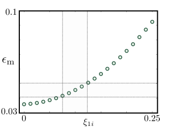
Figure 18: Micromotion error: Scaling of the micromotion error bound $\epsilon_{\rm m}$ with the ratio of the excess micromotion to the laser wavelength $\xi_{1i}$. The shaded area represents the parameters of interest.

Once this has been shown, we must consider the effects of the micromotion on the derivation of the spin-phonon term (12). Following a similar procedure, we obtain the micromotion contributions to the Lamb-Dicke expansion connecting the dipole force (10) to the spin-phonon coupling (12)

$$H_{\rm d}=\frac{\Omega_{\rm L}}{2}\sum_{i,m,p}J_{m}(\xi_{{\rm L}i}){\rm e}^{{\rm i}{\bf k}_{\rm L}\cdot{\bf r}_{i}^{0}}\sigma_{i}^{z}f_{p}(\{a_{n}\}){\rm e}^{{\rm i}(m\Omega_{\rm rf}-\omega_{\rm L})t}+\text{H.c.},$$ (80)

where we have introduced $\xi_{{\rm L}i}=q_{x}{\bf k}_{\rm L}\cdot{\bf r}_{i}^{0}/2$, and

$$f_{p}(\{a_{n}\})=\frac{1}{p!}\left({\rm i}\sum_{n}\eta_{n\bot}\mathcal{M}_{in}^{\bot}\left(a_{n}{\rm e}^{-{\rm i}\Omega_{n}^{\bot}t}+a_{n}^{\dagger}{\rm e}^{{\rm i}\Omega_{n}^{\bot}t}\right)\right)^{p}.$$ (81)

Note that the above expression (80) includes all the possible resonances between the secular and micromotion sidebands with the laser beatnote $\omega_{\rm L}=\omega_{1}-\omega_{2}$. The leading-order term for small Lamb-Dicke parameter $\eta_{n\bot}\ll 1$ occurs for the secular resonance $m=0$, and $p=1$. This term leads directly to the desired spin-phonon coupling (12) provided that

$$\omega_{\rm L}\approx\Omega_{n}^{\bot},\hskip 4.30554pt|\Omega_{\rm L}|\ll\omega_{\rm L}.$$ (82)

Considering the different orders of magnitude in the problem $\omega_{\rm L}/2\pi\approx\omega_{y}/2\pi\approx$10 MHz $\ll\Omega_{\rm rf}/2\pi\approx 0.1$ GHz, the leading micromotion resonance would occur for the term $\Omega_{\rm L}\eta_{n\bot}^{p}J_{m}(\xi_{{\rm L}i}){\rm e}^{{\rm i}(-p\Omega_{n}^{\bot}+m\Omega_{\rm rf}-\omega_{\rm L})t}$ with $m=1$ and $p\approx 9$. Since these terms scale as $(\eta_{n\bot})^{p}$ with $\eta_{n\bot}\ll 1$, they get exponentially suppressed and can be thus neglected. Let us note that the remaining off-resonant sidebands can also be neglected via a RWA in the regime of interest $\Omega_{\rm L}\ll\omega_{\rm L}\ll\Omega_{\rm rf}$. Therefore, we conclude that the micromotion does not modify the spin-phonon coupling (12).

Micromotion contribution to unwanted transitions: Equation (74) implicitly assumes that the dynamics due to the Raman-beam configuration can be accurately described by only three levels $|{\uparrow_{i}}\rangle,|{\downarrow_{i}}\rangle,|r_{i}\rangle$. While this is always true for Zeeman ions, some special care must be taken for hyperfine ones, where the laser beams may excite some of the remaining states of the ground-state manifold due to the extra resonances introduced by the micromotion. Hence, the laser-ion Hamiltonian in Eq. (74) must be supplemented $V+\Delta V$ by

$$\Delta V(t)=\sum_{l,i,a}\frac{\Omega_{l,a}}{2}|r_{i}\rangle\langle a_{i}|{\rm e}^{{\rm i}{\bf k}_{l}\cdot{\bf r}_{i}}{\rm e}^{{\rm i}\xi_{li}\cos\Omega_{\rm rf}t}{\rm e}^{{\rm i}\delta_{l,a}t}+\text{H.c.},$$ (83)

which includes all the additional states $|a_{i}\rangle$ of the ground-state manifold with energies $\epsilon_{a}$, and we have introduced the detunings $\delta_{l,a}=\epsilon_{r}-\epsilon_{a}-\omega_{l}$. These detunings can be controlled by the Zeeman shifts of the ground-state manifold $\{|a_{i}\rangle\}$ caused by an external magnetic field. Note that the aforementioned unwanted transitions that take the state out of the spin subspace $s\in\{\uparrow,\downarrow\}$ follow from two-photon processes evolving like $\Omega_{1,a}\Omega_{2,\uparrow}^{*}J_{m}(\xi_{1i})J_{m^{\prime}}(\xi_{2i})^{*}{\rm e}^{-{\rm i}(\delta_{a,\uparrow}-\omega_{\rm L}-(m-m^{\prime})\Omega_{\rm rf})t}$. Therefore, the Zeeman splittings $\delta_{a,s}=\epsilon_{a}-\epsilon_{s}$ must be tuned to

$$|\Omega_{1,a}\Omega_{2,s}^{*}|\ll|\delta_{a,s}-\omega_{\rm L}\pm\Omega_{\rm rf}|,$$ (84)

such that these unwanted transitions become highly off-resonant and can be neglected in a RWA.

Appendix C Thermal fluctuations and phonon heating

In this appendix, we discuss an alternative derivation of the effective spin models based on the Heisenberg equation of motion, which shall allow us to predict the effects of finite temperatures for the results presented in Sec. III. The starting point is the time-independent spin-phonon Hamiltonian in Eq. (15), rewritten here for convenience

$$\tilde{H}_{\rm p}+\tilde{H}_{\rm d}=\sum_{n}\delta_{n}^{\bot}a_{n}^{\dagger}a_{n}^{\phantom{\dagger}}+\sum_{i,n}(\mathcal{F}_{in}\sigma_{i}^{z}a_{n}^{\dagger}+\text{H.c.}),$$ (85)

where we have introduced $\mathcal{F}_{in}={\rm i}\frac{\Omega_{\rm L}}{2}{\rm e}^{{\rm i}{\bf k}_{\rm L}\cdot{\bf r}_{i}^{0}}\eta_{n\bot}\mathcal{M}_{in}^{\bot}$. In this picture, the evolution of the operators is given by the following system of coupled differential equations

$$\begin{split}\frac{{\rm d}\sigma_{i}^{+}(t)}{{\rm d}t}&=\sigma_{i}^{+}(t)\sum_{n}2{\rm i}(\mathcal{F}_{in}a_{n}^{\dagger}(t)+\mathcal{F}^{*}_{in}a_{n}^{\phantom{\dagger}}(t)),\\ \frac{{\rm d}\hskip 0.43057pta_{n}^{\phantom{+}}(t)}{{\rm d}t}&=-{\rm i}\delta_{n}^{\bot}a_{n}^{\phantom{\dagger}}(t)-{\rm i}\sum_{i}\mathcal{F}_{in}\sigma_{i}^{z}(t),\\ \frac{{\rm d}\sigma_{i}^{z\phantom{i}}(t)}{{\rm d}t}&=0.\end{split}$$ (86)

Thanks to the last conserved quantity $\sigma_{i}^{z}(t)=\sigma_{i}^{z}(0)$, we can integrate this system of equations exactly. The evolution of the phonon operators corresponds to that of a forced quantum harmonic oscillator, namely

$$a_{n}^{\phantom{\dagger}}(t)=a_{n}^{\phantom{\dagger}}(0){\rm e}^{-{\rm i}\delta_{n}^{\bot}t}+\sum_{i}\frac{\mathcal{F}_{in}}{\delta_{n}^{\bot}}\sigma_{i}^{z}(0)\left({\rm e}^{-{\rm i}\delta_{n}^{\bot}t}-1\right).$$ (87)

By substituting on the remaining equation, we find a homogeneous linear differential equation for $\sigma_{i}^{+}(t)$, which can be integrated exactly. We are interested in deriving an estimate for the scaling of the error at finite temperatures

$$\epsilon_{T}=\frac{|\langle\sigma_{i}^{x}\rangle_{T}-\langle\sigma_{i}^{x}\rangle_{T=0}|}{|\langle\sigma_{i}^{x}\rangle_{T=0}|},$$ (88)

where $T$ is the temperature determining the phonon Gibbs state $\rho_{\rm th}=Z^{-1}{\rm e}^{-\beta\sum_{n}\Omega_{n}^{\bot}a_{n}^{\dagger}a_{n}},$ such that $Z={\rm Tr}\{{\rm e}^{-\beta\sum_{n}\Omega_{n}^{\bot}a_{n}^{\dagger}a_{n}}\}$ is the partition function, and $\beta=(k_{\rm B}T)^{-1}$ is expressed in terms of the Boltzman constant $k_{\rm B}$. By considering a separable initial state $\rho(0)=|\psi_{\rm s}\rangle\langle\psi_{\rm s}|\otimes\rho_{\rm th}$, where $|\psi_{\rm s}\rangle$ is a pure spin state, we find the following expression for the relative thermal error

$$\epsilon_{T}=\left(1-{\rm Tr}\left\{\rho_{\rm th}{\rm e}^{\sum_{n}\frac{2\mathcal{F}_{in}}{\delta_{n}^{\bot}}({\rm e}^{{\rm i}\delta_{n}^{\bot}t}-1)a_{n}^{\dagger}-\rm{H.c.}}\right\}\right).$$ (89)

This expectation value can be evaluated exactly to yield the following result

$$\epsilon_{T}=\left(1-{\rm e}^{-\sum_{m}\frac{8|\mathcal{F}_{im}|^{2}}{(\delta_{m}^{\bot})^{2}}\big{(}1-\cos\delta_{m}^{\bot}t\big{)}\bar{n}_{m}^{\bot}}\right),$$ (90)

where the effects of the zero-point motion have been included in $\langle\sigma_{i}^{x}\rangle_{T=0}$, and we have introduced the mean phonon numbers for each of the vibrational modes $\bar{n}_{m}^{\bot}=\langle a_{m}^{\dagger}a_{m}\rangle$. It is interesting to note that, as argued for the so-called quantum phase gates sd_force_review , the error can be minimized by considering evolution times that are multiples of the detuning of the closest vibrational mode $\delta^{\bot}_{m^{*}}$, namely $t_{\rm f}=2\pi n/\delta_{m^{*}}^{\bot}$, where $n\in\mathbb{Z}$.

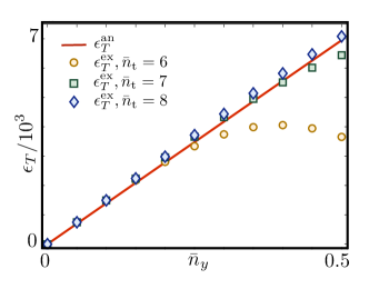
Figure 19: Relative thermal error: Scaling of the relative thermal error $\epsilon_{T}$ with the mean number of phonons in the center-of-mass mode $\bar{n}_{y}$.The analytical estimate $\epsilon_{T}^{\rm an}$ in Eq. (90) (red solid line) is compared to the exact numerical results $\epsilon_{T}^{\rm ex}$ (doted lines) for different truncations of the phonon Hilbert space $\bar{n}_{\rm t}=6,7,8$.

In order to check the validity of our derivation, we have confronted the prediction (90) to the exact time evolution of the spin-phonon model in Eq. (85). We use the parameters of Sec. III, namely, the trap frequency $\omega_{y}/2\pi=20$ MHz, and the laser parameters $\eta_{y}=0.1$, $\omega_{\rm L}=1.1\omega_{y}$, $\Omega_{\rm L}=0.15|\delta_{y}|/\eta_{y}$, and ${\bf e}_{x}\cdot{\bf k}_{\rm L}=0$. In Fig. 19, we represent the exact results for the thermal error $\epsilon_{\rm T}^{\rm ex}$ (dotted lines) obtained by the numerical integration of the Liouville equation ${\rm d}\rho/{\rm d}t=-{\rm i}[\tilde{H}_{\rm p}+\tilde{H}_{\rm d},\rho]$ up to $t_{\rm f}=\pi/8J_{\rm eff}$ for the Hamiltonian (85). Note that we truncate the Hilbert space of each vibrational mode to $\bar{n}_{\rm t}=6$ (yellow circles), $\bar{n}_{\rm t}=7$ (green squares), and $\bar{n}_{\rm t}=8$ (blue diamonds). These results are compared to the analytical estimate $\epsilon_{\rm T}^{\rm an}$ (red solid line) in Eq. (90), showing a remarkable agreement for a sufficiently large truncation of the phonon Hilbert space.

We now derive a useful expression for the scaling of the error in terms of experimental parameters, in the limit of $|\mathcal{F}_{in}|\ll\delta_{n}^{\bot}$. We perform a Taylor expansion of Eq. (90) for $\kappa_{y}\ll 1$, and take into account the orthonormality properties of the normal-mode displacements $\mathcal{M}_{in}^{\bot}$. For low- and high-temperatures, we have $\bar{n}_{n}^{\bot}\approx\beta\Omega_{n}^{\bot}$ and $\bar{n}_{n}^{\bot}\approx(\beta\Omega_{n}^{\bot})^{-1}$ respectively, where $\beta=1/k_{\rm B}T$. In both regimes, we find the following upper bound for the error

$$\epsilon_{T}\leq\epsilon_{\rm th}={\rm max}_{t}\{\epsilon_{T}\}=\left(1-{\rm e}^{-\frac{4|\Omega_{\rm L}|^{2}\eta_{y}^{2}}{\delta_{y}^{2}}\bar{n}_{y}}\right),$$ (91)

where we have introduced $\bar{n}_{y}=(\beta\omega_{y})$, which corresponds to the mean phonon number for the center-of-mass mode. Finally, in the low-temperature regime, one finds

$$\epsilon_{T}\leq\epsilon_{\rm th}=\frac{4|\Omega_{\rm L}|^{2}\eta_{y}^{2}}{\delta_{y}^{2}}\bar{n}_{y}$$ (92)

By controlling the experimental parameters, this error term should be minimized for the QS. Note that this linear scaling of the relative error with the mean number of phonons coincides with the results shown in Fig. 19.

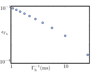
Figure 20: Relative heating error: Scaling of the relative heating error $\epsilon_{\Gamma_{\rm h}}$ with the inverse of the heating rate $\Gamma_{\rm h}^{-1}$ (logarithmic scale).

Another important question to address is the error caused by heating mechanisms. The heating of a particular vibrational mode may be induced by a variety of factors, such as the combination of stray electric fields and fluctuating trap parameters, elastic collisions with a background gas, fluctuating patch fields in the trap electrodes, or non-linear static electric fields (see ion_trap_reviews for details). Therefore, we shall not focus on a particular microscopic model, but use instead a phenomenological master equation

$$\frac{{\rm d}\rho}{{\rm d}t}=-{\rm i}[\tilde{H}_{\rm p}+\tilde{H}_{\rm d},\rho(t)]+\mathcal{D}_{\rm h}(\rho(t)),$$ (93)

where the coherent dynamics is given by Eq. (85), and the heating dissipator corresponds to

$$\mathcal{D}_{\rm h}(\rho)=\sum_{n}\Gamma_{\rm h}\left(a_{n}^{\dagger}\rho a_{n}-\textstyle\frac{1}{2}a_{n}a_{n}^{\dagger}\rho-\textstyle\frac{1}{2}\rho a_{n}a_{n}^{\dagger}\right).$$ (94)

Here, we have considered that the heating rate $\Gamma_{\rm h}$ is equal for all the vibrational modes. In addition to Eq. (90), the heating mechanism provides another source of error. In order to single out such a contribution, we consider an initially ground-state-cooled ion crystal, and integrate numerically the above master equation. To estimate the relative error caused by the heating mechanism, we evaluate the following figure of merit

$$\epsilon_{{\rm h}}=\frac{|\langle\sigma_{i}^{x}\rangle_{\Gamma_{\rm h}}-\langle\sigma_{i}^{x}\rangle_{\Gamma_{\rm h}=0}|}{|\langle\sigma_{i}^{x}\rangle_{\Gamma_{\rm h}=0}|}.$$ (95)

By considering a small timescale $t_{\rm f}\ll(\Gamma_{\rm h})^{-1}$, the evolution of the mean number of phonons due to the dissipator (94) yields a simple linear heating $\bar{n}^{\bot}_{n}(t)=\langle a_{n}^{\dagger}a_{n}\rangle\approx\Gamma_{\rm h}t$. We set $t_{\rm f}=1\pi/(8J_{\rm eff})$, in such a way that $\bar{n}^{\bot}_{n}(t)\ll\bar{n}_{\rm t}=2$. The remaining parameters are the same as above. In Fig. 20, we represent the relative error (95) as a function of the inverse heating rate $\Gamma_{\rm h}^{-1}$, which sets the timescale for the creation of one vibrational excitation. As can be seen in this figure, heating times above 5 ms/ phonon, only have a small contribution (1%) to the overall error of the QS.

References

- (1) P. W. Anderson, Science 177, 393 (1972).
- (2) X. Wen, Quantum Field Theory of Many-body Systems (Oxford Univ. Press, New York, 2004).
- (3) R. P. Feynman, Int. J. Theo. Phys. 21, 467 (1982); S. Lloyd, Science 273, 1073 (1996).
- (4) I. Buluta and F. Nori, Science 326, 108 (2009).
- (5) Insight on Quantum Simulation, Nat. Phys. 8, 263-299 (2012).
- (6) D. J. Wineland, et al., J. Res. Natl. Inst. Stand. Tech. 103, 259 (1998); D. Leibfried, et al., Rev. Mod. Phys. 75, 281 (2003); H. Haeffner, et al., Phys. Rep. 469, 155 (2008).
- (7) J. T. Barreiro et al., Nature 470, 486 (2011); B. P. Lanyon, et al. Science 334, 57 (2011).
- (8) A. Friedenauer, et al., Nat. Phys. 4, 757 (2008); K. Kim, et al., Phys. Rev. Lett. 103, 120502 (2009); E. E. Edwards, et al., Phys. Rev. B 82, 060412(R) (2010).
- (9) K. Kim, et al., Nature 465, 590 (2010).
- (10) R. Islam, et al., Nat. Comm. 2, 377 (2011).
- (11) R. Gerritsma, et al., Nature 463, 68 (2010); R. Gerritsma, et al., Phys. Rev. Lett. 106, 060503, (2011).
- (12) J. W. Britton, B. C. Sawyer, A. C. Keith, C.-C. J. Wang, J. K. Freericks, H. Uys, M. J. Biercuk and J. J. Bollinger, Nature 484, 489 (2012).
- (13) M. Johanning, A. F. Varon, and C. Wunderlich, J. Phys. B. 42, 154009 (2009); C. Schneider, D. Porras, and T. Schaetz, Rep. Prog. Phys. 75, 024401 (2012).
- (14) L. Lamata, J. Leon, T. Schaetz, and E. Solano, Phys. Rev. Lett. 98, 253005 (2007); A. Bermudez, M.A. Martin-Delgado, and E. Solano, Phys. Rev. A 76, 041801 (R) (2007); N. C. Menicucci and G. J. Milburn, Phys. Rev. A 76, 052105 (2007); R. Schützhold, et al., Phys. Rev. Lett. 99, 201301 (2007); A. Bermudez, M.A. Martin-Delgado, and A. Luis, Phys. Rev. A 77, 033832 (2008); B. Horstmann, B. Reznik, S. Fagnocchi, and J. I. Cirac, Phys. Rev. Lett. 104, 250403 (2010); J. Casanova et al., Phys. Rev. X. 1, 021018 (2011); J. Casanova, et al., Phys. Rev. Lett. 107, 260501 (2011); M. del Rey, D. Porras, and E. Martin-Martinez, Phys. Rev. A 85, 022511 (2012).
- (15) D. Porras and J.I. Cirac, Phys. Rev. Lett. 92, 207901 (2004); X.-L. Deng, D. Porras, and J. I. Cirac, Phys. Rev. A 72, 063407 (2005).
- (16) M. Pons, et al., Phys. Rev. Lett. 98, 023003 (2007); A. Bermudez, D. Porras, and M. A. Martin-Delgado, Phys. Rev. A 79, 060303 (R) (2009); P. Hauke, et al., New J. Phys. 12, 113037 (2010); P. A. Ivanov and F. Schmidt-Kaler, New J. Phys. 13, 125008 (2011); R. Schmied, J. H. Wesenberg, and D. Leibfried, New J. Phys. 13, 115011 (2011).
- (17) G.-D. Lin, C. Monroe, and L.-M. Duan, Phys. Rev. Lett. 106, 230402 (2011)
- (18) A. Bermudez, et al., Phys. Rev. Lett. 107, 207209 (2011).
- (19) D. Porras and J.I. Cirac, Phys. Rev. Lett. 93, 263602 (2004); X.-L. Deng, D. Porras, and J.I. Cirac, Phys. Rev. A 77, 033403 (2008); R. Schmied, et al., New J. Phys. 10, 045017 (2008); A. Bermudez, M. A. Martin-Delgado, and D. Porras, New J. Phys. 12, 123016 (2010); A. Bermudez, T. Schaetz, and D. Porras, Phys. Rev. Lett. 107, 150501 (2011); A. Bermudez, T. Schaetz, and D. Porras, New J. Phys. 14, 05304 (2012).
- (20) D. Porras, F. Marquardt, J. von Delft, and J.I. Cirac, Phys. Rev. A 78, 010101 (R) (2008); P. A. Ivanov, et al., Phys. Rev. A 80, 060301(R) (2009); D. Porras, P. A. Ivanov, and F. Schmidt-Kaler, Phys. Rev. Lett. 108, 235701 (2012; A. Bermudez and M. B. Plenio, Phys. Rev. Lett. 109, 010501 (2012).
- (21) I. García-Mata, O. V. Zhirov, and D. L. Shepelyansky, Eur. Phys. J. D 41, 325 (2007); A. Benassi, A. Vanossi, and E. Tosatti, Nat. Commun. 2, 236 (2011); T. Pruttivarasin, et al., New J. Phys. 13 075012 (2011); G.-D. Lin and L.-M. Duan, New J. Phys. 13, 075015 (2011).
- (22) P. Lechemitant, in Frustrated spin systems, edited by H. T. Diep, (World-Scientific, Singapore, 2004).
- (23) S. Sachdev, Quantum Phase Transtions, (Cambridge University Press, Cambridge, 1999).
- (24) P. W. Anderson, Science 235, 1196 (1987).
- (25) P. Pfeuty, Ann. Phys. 57, 79 (1970).
- (26) P. Lemmens, G. Guntherodt, and C. Gros, Phys. Rep. 375, 1 (2003).
- (27) R. Coldea, et al., Science 327, 177 (2010).
- (28) We note that the spin model for the cobalt niobate is not strictly one-dimensional, but corresponds to a three-dimensional model of ferromagnetic Ising chains weakly coupled in a triangular lattice cobalt_balents . A more realistic model for the chains includes a weak transverse exchange typical of Heisenberg magnets. See the supporting online material of tfi_solid . Besides, there is also an antiferromagnetic nearest-neighbor Ising coupling cobalt_moore . However, this coupling is sufficiently weak so that its consequences to the magnetic frustration are not relevant.
- (29) S. Lee, R. K. Kaul, and L. Balents, Nat. Physics 6, 702 (2010).
- (30) J. A. Kjäll, F. Pollmann, and J. E. Moore, Phys. Rev. B 83, 020407 (R) (2011).
- (31) J. Simon, et al., Nature 472, 307 (2011).
- (32) G. H. Wannier, Phys. Rev. 79, 357 (1950).
- (33) S. T. Bramwell, and M. J. P. Gingras, Science 294, 1495 (2001); R. Moessner and A. P. Ramirez, Phys. Today 59, 24 (2006).
- (34) A. Dutta, et al., Transverse field spin models: From Statistical Physics to Quantum Information, arXiv:1012.0653 (2010).
- (35) A. P. Ramirez, Annu. Rev. Mat. Sci. 24, 453 (1994).
- (36) R. Liebmann, Statistical Mechanics of Periodic Frustrated Ising Systems, (Springer-Verlag, New York, 1986).
- (37) R. Moessner, S. L. Sondhi, and P. Chandra, Phys. Rev. Lett. 84, 4457 (2000); R. Moessner and S. L. Sondhi, Phys. Rev. B 63, 224401 (2001).
- (38) E. Dagotto and T. M. Rice, Science 271, 618 (1996).
- (39) J.G. Bednorz and K.A. Muller, Z. Phys. B 64, 188 (1986)
- (40) G. Sierra, in Lecture Notes in Physics, vol. 478, eds. G. Sierra, and M.A. Martin-Delgado, (Springer-Verlag, Berlin, 1997).
- (41) F. Diedrich, et al., Phys. Rev. Lett. 59, 2931 (1987); D. J. Wineland, et al., Phys. Rev. Lett. 59, 2935 (1987).
- (42) I. Waki, S. Kassner, G. Birkl, and H. Walther, Phys. Rev. Lett. 68, 2007 (1992); M. Drewsen, et al., Phys. Rev. Lett. 81, 2878 (1998); L. Hornekaer, N. Kjaergaard, A. M. Thommesen, and M. Drewsen, Phys. Rev. Lett. 86, 1994 (2001); N. Kjaergaard and M. Drewsen, Phys. Rev. Lett. 91, 095002 (2003); A. Mortensen, E. Nielsen, T. Matthey, and M. Drewsen, Phys. Rev. Lett. 96, 103001 (2006).
- (43) J. P. Schiffer, Phys. Rev. Lett. 70, 818 (1993); D. H. E. Dubin, Phys. Rev. Lett. 71, 2753 (1993).
- (44) G. Birkl, S. Kassner, and H. Walther, Nature 357, 310 (1992); D. G. Enzer, et al., Phys. Rev. Lett. 85, 2466 (2000); T. Schaetz, U. Schramm, and D. Habs, Nature 412, 717 (2001).
- (45) S. Fishman, G. De Chiara, T. Calarco, and G. Morigi, Phys. Rev. B 77, 064111 (2008); A. Retzker, R. C. Thompson, D. M. Segal, and M. B. Plenio, Phys. Rev. Lett. 101, 260504 (2008); Z-X. Gong, G.-D. Lin, and L.-M. Duan, Phys. Rev. Lett. 105, 265703 (2010); E. Shimshoni, G. Morigi, and S. Fishman, Phys. Rev. Lett 106, 010401 (2011); R. Nigmatullin, et al., arXiv:1112.1305 (2011).
- (46) A. del Campo, et al., Phys. Rev. Lett. 105, 075701 (2010).
- (47) J. Chiaverini and W.E. Lybarger Jr., Phys. Rev. A 77, 022324 (2008); J. Labaziewicz et al., Phys. Rev. Lett. 100, 013001 (2008); R. Schmied, J.H. Wesenberg, and D. Leibfried, Phys. Rev. Lett. 102, 233002 (2009); N. Daniilidis et al., New J. Phys. 13, 013032 (2011); G. R. Brady et al., arXiv:1008.2977 (2010); J. J. McLoughlin et al., Phys. Rev. A 83, 013406 (2011).
- (48) R. P. Feynman, Statistical Mechanics: A Set Of Lectures (Ben- jamin/Cummings Publishing, Massachusetts, 1972).
- (49) J.I. Cirac, and P. Zoller, Nature 404, 579 (2000); G. J. Milburn, S. Schneider, and D. F. V. James, Fortschr. Phys. 48, 801 (2000); C. Wunderlich, Laser Physics at the Limit, p. 261 (Berlin, Springer, 2002).
- (50) C. Monroe, et al., Science 272, 1131 (1996); D. Leibfried, et al., Nature 422, 412 (2003); P. C. Haljan, et al., Phys. Rev. Lett 94, 153602 (2005); U. G. Poschinger, A. Walther, K. Singer, and F. Schmidt-Kaler, Phys. Rev. Lett. 105, 263602 (2010).
- (51) K-A Brickman Soderberg and C. Monroe, Rep. Prog. Phys. 73 036401(2010).
- (52) For optical ions, such as , it is possible to use a single-photon scheme and implement the spin couplings via a pair of sidebands according to the Mølmer-Sørensen scheme. However, once the direction of the beams is fixed, the ratio of their wavelength to the mutual ion distance, which determines the anisotropy of the spin couplings, cannot be modified further.
- (53) C. Ospelkaus, et al., Nature 476, 181 (2011); A. Khromova, et al., Phys. Rev. Lett. 108, 220502 (2012).
- (54) M. A. Ruderman and C. Kittel, Phys. Rev. 96, 99 (1954); T. Kasuya, Prog. Theor. Phys. 16, 45 (1956); K. Yosida, Phys. Rev. 106, 893 (1957).
- (55) The canonical transformation in Eq. (14) resembles the so-called Lang-Firsov transformation customary of polaron physics (see polaron_book and references therein). This spin-dependent displacement was first used in the field of paramagnetic salts with impurities kanamori (see also elliot ). In the context of trapped ions, it has been exploited for quantum-logic spin_displacement_wunderlich , and quantum simulations purposes ising_porras .
- (56) A. S. Alexandrov and J. T. Devreese, Advances in Polaron Physics, (Springer-Verlag, Berlin, 2010)
- (57) J. Kanamori, J. Appl. Phys. 31, S14 (1960).
- (58) R. J. Elliot, et al., J. Phys. C 4, L179 (1971)
- (59) F. Mintert and C. Wunderlich, Phys. Rev. Lett. 87 257904 (2001).
- (60) G. Toulouse, Commun. Phys. 2, 115 (1977); J. Villain, J. Phys. C 10, 1717 (1977).
- (61) S. M. Giampaolo, G. Gualdi, A. Monras, and F. Illuminati, Phys. Rev. Lett. 107, 260602 (2011).
- (62) S. Korenblit, et al., arXiv:1201.0776 (2012).
- (63) D. T. Gillespie, Am. J. Phys. 64, 3 (1996).
- (64) K. Singer, et al., Rev. Mod. Phys. 82, 2609 (2010).
- (65) C. F. Roos, et al., Phys. Rev. Lett. 85, 5547 (2000); F. Schmidt-Kaler, et al. Appl. Phys. B 73, 807 (2001).
- (66) S. Schulz et al., Fortschr. Phys. 54, 648 (2006).
- (67) M. Paris and J. Rehacek, eds., Quantum State Estimation, (Springer, Heidelberg, 2004).
- (68) M. Cramer et al., Nat. Commun. 1, 149 (2010); T. Baumgratz, D. Gross, M. Cramer and M.B. Plenio, arXiv:1207.0358 (2012).
- (69) R. H. Lehmberg, Phys. Rev. A 2, 883 (1970); G. S. Agarwal, Quantum Statistical Theories of Spontaneous Emission and their Relation to Other Approaches, (Springer, Berlin, 1974).
- (70) I. de Vega, J. I. Cirac, and D. Porras, Phys. Rev. A 77, 051804(R) (2008).
- (71) M. Cramer, M.B. Plenio, and H. Wunderlich, Phys. Rev. Lett. 106, 020401 (2011).
- (72) D. J. Berkeland, et al., J. Appl. Phys. 83, 5025 (1998).
- (73) N. Timoney, et al., Nature 476, 185 (2011).
- (74) A. Bermudez, P. O. Schmidt, M. B. Plenio, and A. Retzker, Phys. Rev. A 85, 040302(R) (2012).
- (75) M. B. Plenio and P. Knight, Phys. Rev. A 53, 2986 (1996); M. B. Plenio and P. Knight, Proc. Roy. Soc. A 453, 2017 (1997).
- (76) R. Ozeri, et al., Phys. Rev. Lett. 95, 030403 (2005).
- (77) H. Uys, et al., Phys. Rev. Lett. 105, 200401 (2010).
- (78) R. J. Elliot, Phys. Rev. 124, 346 (1961); ; M.E. Fisher and W. Selke, Phys. Rev. Lett. 44, 1502 (1980).
- (79) The full phase diagram of the -QIM is spanned by the ratios , and . However, in the absence of a longitudinal field, it suffices to restrict to , such that the model consists of competing nearest-neighbor ferromagnetic interactions , and next-to-nearest neighbor antiferromagnetic ones . The magnetic phases with can be obtained by a inversion that only involves next-to-nearest neighboring spins.
- (80) H. Uys, M. J. Biercuk, J. Britton, and J. J. Bollinger, Toward Spin Squeezing with Trapped Ions, arXiv:1111.4792 (2011).
- (81) D. Porras and J.I. Cirac, Phys. Rev. Lett. 96, 250501 (2006).
- (82) R. Moessner and K. S. Raman, in Introduction to Frustrated Magnetism, Eds. C. Lacroix, P. Mendels, and F. Mila (Springer Series in Solid-State Sciences, Berlin 2011).
- (83) D. S. Rokhsar and S. A. Kivelson, Phys. Rev. Lett. 61, 2376 (1998).
- (84) J. Villain, R. Bidaux, J.-P. Carton and R. Conte, J. Physique 41, 1263 (1980).
- (85) L. Balents, Nature 464, 199 (2010).
- (86) D. J. Priour, M. P. Gelfand, and S. L. Sondhi, Phys. Rev. B 64, 134424 (2001).
- (87) W. H. Zurek, U. Dorner, and P. Zoller, Phys. Rev. Lett. 95, 105701 (2005); A. Bermudez, D. Patane, L. Amico, and M. A. Martin-Delgado, Phys. Rev. Lett. 102, 135702 (2009); J. Dziarmaga, W. H. Zurek, and M. Zwolak, Nat. Physics 8, 49 (2012).
- (88) W. Selke, Phys. Rep. 170, 213 (1988).
- (89) S. Redner, J. Stat. Phys. 25, 15 (1981).
- (90) M. N. Barber and P. M. Duxbury, J. Phys. A 14, L251 (1981).
- (91) P. Bak, Rep. Prog. Phys. 45, 587 (1989).
- (92) W. Selke and M. E. Fisher, Z. Phys. B 40, 71 (1980); W. Selke, Z. Phys. B 43, 335 (1981).
- (93) J. Villain and P. Bak, J. Physique 42, 657 (1981).
- (94) D. Allen, P. Azaria, and P. Lecheminant, J. Phys. A 34, L305 (2001).
- (95) M. Beccaria, M. Campostrini, and A. Feo, Phys. Rev. B 73, 052402 (2006); ibid 76, 094410 (2007).
- (96) J. M. Kosterlitz and D. J. Thouless, J. Phys. C 6, 1181 (1973).
- (97) V. L. Pokrovsky and A. L. Talapov, Phys. Rev. Lett. 42, 65 (1979).
- (98) H. C. Nägerl, et al., Phys. Rev. A 60, 145 (1999).
- (99) F. Reitner and A. S. Sørensen, Phys. Rev. A 85, 032111 (2012).
- (100) O. K. Gosh, Ion Traps, (Oxford University Press, USA ,1996).
- (101) J. P. Schiffer, M. Drewsen, J. S. Hangst, and L. Hornekaer, Proc. Natl. Acad. Sci. USA 97 10697 (2000).
- (102) V. L. Ryjkov, X. Zhao, and H. A. Schuessler, Phys. Rev. A 71, 033414 (2005).
- (103) Q. A. Turchette, et al., Phys. Rev. Lett. 81, 3631 (1998).
- (104) H. Kaufmann, et al., arXiv:1208.4040 (2012).
- (105) H. Landa, M. Drewsen, B. Reznik, A. Retzker, arXiv:1206.4006 (2012).
- (106) R. G. DeVoe, J. Hoffnagle, and R. G. Brewer, Phys. Rev. A 39, 4362 (1989).