A Comprehensive Analysis of Time Series Segmentation on the Japanese Stock Prices

Abstract

This study conducts a comprehensive analysis of time series segmentation on the Japanese stock prices listed on the first section of the Tokyo Stock Exchange during the period from 4 January 2000 to 30 January 2012. A recursive segmentation procedure is used under the assumption of a Gaussian mixture. The daily number of each quintile of volatilities for all the segments is investigated empirically. It is found that from June 2004 to June 2007, a large majority of stocks are stable and that from 2008 several stocks showed instability. On March 2011, the daily number of instable securities steeply increased due to societal turmoil influenced by the East Japan Great Earthquake. It is concluded that the number of stocks included in each quintile of volatilities provides useful information on macroeconomic situations.

1 Introduction

Recently, interests in a relationship between price movements and events or news seem to increase Kenett:12; Ilaria; Preis. The traded prices are assumed to be signals resulting from both exogenous and endogenous factors.

Agent-based models of financial markets have been developed for the last decade Zhang:98; Challet:00; Bornholdt:01; Krawiecki:02; Alfrano:2005; Feng. Normally buyers and sellers are assumed in the model. A market including several agents is considered. Fundamentalists, chartists, and noise traders may interplay in financial markets. The fundamentalists know actual value of stock but the actual value fluctuates in time. The chartists watch price movements and determine their prices based on the price movements. The chartists are classified into trend followers and contrarians. The noise traders determine their trading prices randomly. As modelled above, the financial market consists of various types of participants is a kind of agent-based information processing systems embedded in the real world.

In the last two decades, statistical properties of asset price returns have been successively studies in the literature of econophysics Mantegna ; Bouchaud . One of the important properties is that the probability distribution of returns exhibits a fat-tailed distribution Mandelbrot ; Gopikrishnan . Several researchers reported that the tail distributions of log returns have the power-law and are well fitted by Student’s $t$-distributions Praetz or $q$-Gaussian distributions founded in nonextensive statistical thermo dynamics Tsallis ; Aki-Hiro:10 . The Beck model introduced as a dynamical foundation of Tsallis statistics Beck:Dyn Although it is originally intended to describe mechanical systems such as turbulence, its basic idea of fluctuating temperature is well consistent with the heteroscedasticity of markets. Thus, in recent studies, it is employed to elucidate price fluctuations in markets Kozuki ; Ausloos and it is called superstatistics Beck:Sup . Moreover, the boom-bust cycle is associated with the existence of bubbles in stock markets. This cycle may be quantified by collective behavior of stock prices. Researchers have shown that there is some degree of collective behavior and synchronization in the return of actual stocks Shapira.

Macroeconomics situations strongly influence money flows at all the levels of society. Stocks at each sector are traded by investors and traders through the stock exchange markets every minute. Moreover, stock prices are so sensitive to the money flows that stock prices of all the sectors depend on demand-supply situations of the money by economic actors. Therefore, they are expected to be useful for detecting a changes of macroeconomic situations.

In this study, we hope to provide some insights on the problem on quantification of Japanese macroeconomic situations through a comprehensive analysis of stock prices traded in the Tokyo Stock Exchange. In the context of economics and finance, there are various methods to segment highly nonstationary financial time series into stationary segments called regimes or trends. Following the pioneering works by Goldfeld and Quandt Goldfeld , there is an enormous literature on detecting structural breaks or change points separating stationary segments. Recently, a recursive entropic scheme to segment financial time series was proposed Siew:11 . In fact they investigate segments for Japanese stock indices, however, they did not consider stock prices themselves.

A recursive segmentation procedure is applied to analyze security prices of 1,413 Japanese firms listed on the first section of the Tokyo Stock Exchange. In this paper, the number of segments in quintiles in terms of variance is computed in order to detect change points of money flows of the Japanese security market.

This article is organized as follows. In Sec. 2, the recursive segmentation procedure is briefly explained. In Sec. 3 the segmentation procedure is performed for artificial time series. In Sec. 4, the empirical analysis with daily log-returns for the last 10 years is conducted. Sec. 5 is devoted to conclusion.

2 Method

2.1 Segmentation procedure

Let $O_{i,t}$ and $E_{i,t}$ be, respectively, daily opening and closing prices of $i$-th stock $(i=1,\ldots,M)$ at day $t\quad(t=1,\ldots,n)$. $M$ and $n$ are denoted as the total number of stock and the total number of observations. The daily log-return (opening to closing) time series $x_{i,t}\quad(i=1,\ldots,M;t=1,\ldots,n)$ is computed as

$$x_{i,t}=\log E_{i,t}-\log O_{i,t}.$$ (1)

According to the seminal work by Mantegna and Stanley Mantegna , the log-return time series of stock prices are modeled by Lévy distributions. Superstatistics suggests that a mixture of Gaussian distributions with $\chi^{2}$-distributions in terms of variance gives a Lévy distribution. Therefore, we may assume that each segment is sampled from a Gaussian distribution with different mean and variance. Namely, it is assumed that the log-return time series consist of $m_{i}$ stationary segments. Each segment follows a stationary Gaussian distribution with mean $\mu_{i,j}$ and variance $\sigma_{i,j}^{2}$ ($j=1,\ldots,m_{i}$).

To find the $m_{i}-1$ unknown segment boundaries $t_{i,j}$ separating segment $j$ and $j+1$, the recursive segmentation scheme introduced by Siew et al and Bernaola et al Siew:11 ; Bernaola . Their segmentation scheme is fundamentally based on the likelihood-ratio test under an i.i.d Gaussian null model and a joint consisting two different Gaussian models for the total time series.

Firstly, suppose that there are $n$ observations $x_{s}\quad(s=1,\ldots,n)$. Let $g(x;\mu,\sigma^{2})$ be a Gaussian distribution

$$g(x;\mu,\sigma^{2})=\frac{1}{\sqrt{2\pi\sigma^{2}}}\exp\Bigl{[}-\frac{(x-\mu)^{2}}{2\sigma^{2}}\Bigr{]},$$ (2)

with parameters $\mu$ and $\sigma^{2}$. Assuming that the observations $x_{s}$ should be segmented at $t$ and that the observations on the left hand side are sampled from $g(x;\mu_{L},\sigma_{L}^{2})$, and ones on the right hand side are from $g(x;\mu_{R},\sigma_{R}^{2})$, we define likelihood functions

$$L_{1} = \prod_{s=1}^{n}g(x_{s};\mu,\sigma^{2}),$$ (3)

$$L_{2}(t) = \prod_{s=1}^{t}g(x_{s};\mu_{L},\sigma_{L}^{2})\prod_{s=t+1}^{n}g(x_{s};\mu_{R},\sigma_{R}^{2}).$$

Furthermore, we define the logarithmic likelihood-ratio between $L_{1}$ and $L_{2}(t)$ as,

$$\Delta(t)=\log L_{2}(t)-\log L_{1}\Bigr{.}$$ (5)

Inserting Eq. (2) into Eq. (5) we have

$$\Delta(t)=\sum_{s=1}^{t}\log g(x_{s};\mu_{L},\sigma^{2}_{L})+\sum_{s=t+1}^{n}\log g(x_{s};\mu_{R},\sigma^{2}_{R})-\sum_{s=1}^{n}\log g(x_{s};\mu,\sigma^{2}).$$ (6)

By using the approximations

$$\frac{1}{n}\sum_{s=1}^{n}\log g(x_{s};\mu,\sigma^{2}) \approx \int_{-\infty}^{\infty}g(x;\mu,\sigma^{2})\log g(x;\mu,\sigma^{2})\mbox{d}x=-\frac{1}{2}\log\Bigl{(}2\pi e\sigma^{2}\Bigr{)},$$

$$\frac{1}{t}\sum_{s=1}^{t}\log g(x_{s};\mu_{L},\sigma_{L}^{2}) \approx \int_{-\infty}^{\infty}g(x;\mu_{L},\sigma_{L}^{2})\log g(x;\mu_{L},\sigma_{L}^{2})\mbox{d}x=-\frac{1}{2}\log\Bigl{(}2\pi e\sigma_{L}^{2}\Bigr{)},$$

$$\frac{1}{n-t}\sum_{s=t+1}^{n}\log g(x_{s};\mu_{R},\sigma_{R}^{2}) \approx \int_{-\infty}^{\infty}g(x;\mu_{R},\sigma_{R}^{2})\log g(x;\mu_{R},\sigma_{R}^{2})\mbox{d}x=-\frac{1}{2}\log\Bigl{(}2\pi e\sigma_{R}^{2}\Bigr{)},$$

$\Delta(t)$ is rewritten as

$$\Delta(t)=n\log\sigma-t\log\sigma_{L}-(n-t)\log\sigma_{R}\geq 0.$$ (7)

$\sigma$, $\sigma_{L}$ and $\sigma_{R}$ are further approximated as maximum likelihood estimators given by empirical standard deviations

$$\sigma = \sqrt{\frac{1}{n}\sum_{s=1}^{n}x^{2}_{s}-\Bigl{(}\frac{1}{n}\sum_{s=1}^{n}x_{s}\Bigr{)}^{2}},$$ (8)

$$\sigma_{L} = \sqrt{\frac{1}{t}\sum_{s=1}^{t}x^{2}_{s}-\Bigl{(}\frac{1}{t}\sum_{s=1}^{t}x_{s}\Bigr{)}^{2}},$$ (9)

$$\sigma_{R} = \sqrt{\frac{1}{n-t}\sum_{s=t+1}^{n}x^{2}_{s}-\Bigl{(}\frac{1}{n-t}\sum_{s=t+1}^{n}x_{s}\Bigr{)}^{2}}.$$ (10)

$\Delta(t)$ can be used as an indicator to separate the observations into two parts. An adequate way to separate the observations is that segmentation is conducted at $t$ where $\Delta(t)$ takes the maximum value. Namely, an adequate segmentation should be done at

$$t^{*}=\arg\max\Delta(t).$$ (11)

If $\max\Delta(t)$ is less than a threshold value $\Delta_{c}$, then the segmentation should be terminated. The hierarchical segmentation procedure is also applied to the time series. After segmentation, we also apply this procedure for each segment recursively. In order to stop the segmentation procedure we assume that the minimum value $\Delta_{c}$. If $\max\Delta(t)$ is less than $\Delta_{c}$, then we do not apply the segmentation procedure any more. This is used as the stopping condition of the recursive segmentation procedure. Statistical theory tells us that as the sample size $t$ approaches $\infty$, $2\Delta(t)$ is asymptotically $\chi^{2}$ distributed with degrees of freedom equal to the difference between the number of alternative model parameters and the number of null model parameters. In this Gaussian case, the degrees of freedom is set as $2=4-2$. The cumulative distribution of $\chi^{2}(x,2)$ is given by

$$F(x)=1-\exp\bigl{(}-\frac{x}{2}\bigr{)}.$$ (12)

Therefore, for the level of significance $\alpha(0<\alpha<1)$, the threshold is given as

$$\Delta_{c}=-2\log(1-\alpha).$$ (13)

Consequently, for stock $i\quad(i=1,\ldots,M)$, we obtain $m_{i}$ segments and $m_{i}$ sets of Gaussian parameters $\{\mu_{i,j},\sigma_{i,j}^{2}\}\quad(j=1,\ldots,m_{i})$.

2.2 General case

More generally, let us define the discriminator $\Delta(t)$ given in Eq. (7). Assume that $p(x;\theta)$ is a probability density function (model) parameterized by $\theta$. Let $\hat{\theta}$, $\hat{\theta}_{L}$, and $\hat{\theta}_{R}$ be maximum likelihood functions computed by

$$\hat{\theta} = \arg\max_{\theta}\sum_{s=1}^{n}\log p(x_{s};\theta),$$ (14)

$$\hat{\theta}_{L} = \arg\max_{\theta}\sum_{s=1}^{t}\log p(x_{s};\theta),$$ (15)

$$\hat{\theta}_{R} = \arg\max_{\theta}\sum_{s=t+1}^{n}\log p(x_{s};\theta).$$ (16)

where $\hat{\theta}_{L}$ and $\hat{\theta}_{R}$ are maximum likelihood estimators in left and right sequences, respectively. Assuming likelihood functions

$$L_{1} = \prod_{s=1}^{n}p(x_{s};\theta),$$ (17)

$$L_{2}(t) = \prod_{s=1}^{t}p(x_{s};\theta_{L})\prod_{s=t+1}^{n}p(x_{s};\theta_{R}),$$ (18)

we can rewrite Eq. (5) as

$$\Delta(t) = -n\int_{-\infty}^{\infty}p(x;\hat{\theta})\log p(x;\hat{\theta})dx$$ (19)

$$+ t\int_{-\infty}^{\infty}p(x;\hat{\theta}_{L})\log p(x;\hat{\theta}_{L})dx+(n-t)\int_{-\infty}^{\infty}p(x;\hat{\theta}_{R})\log p(x;\hat{\theta}_{R})dx,$$

$\Delta(t)/n$ is equivalent to

$$\frac{\Delta(t)}{n}=H\Bigl{[}p(x;\hat{\theta})\Bigr{]}-\frac{t}{n}H\Bigl{[}p(x;\hat{\theta}_{L})\Bigr{]}-\frac{n-t}{n}H\Bigl{[}p(x;\hat{\theta}_{R})\Bigr{]},$$ (20)

where $H[p(x;\theta)]$ represents the notation of Shannon entropy defined as

$$H\Bigl{[}p(x)\Bigr{]}=-\int_{-\infty}^{\infty}p(x;\theta)\log p(x;\theta)dx.$$ (21)

In this Gaussian case, the degrees of freedom $k$ is set as the dimensionality of a set of model parameters $\theta$. The cumulative distribution of $\chi^{2}$ distribution with degrees of freedom $k$ is given as the regularized incomplete gamma function,

$$F(x)=\gamma\Bigl{(}\frac{k}{2},\frac{x}{2}\Bigr{)}=\frac{1}{\Gamma\bigl{(}\frac{k}{2}\bigr{)}}\int_{0}^{\frac{x}{2}}t^{\frac{k}{2}-1}\exp(-t)dt.$$ (22)

The threshold for the terminated condition under a given level of significance $\alpha$ is calculated from the regularized incomplete gamma function, such that

$$\gamma\Bigl{(}\frac{k}{2},\frac{\Delta_{c}}{2}\Bigr{)}=\alpha.$$ (23)

3 Numerical study

Artificial time series are generated from i.i.d standard normal random variables with different variances. Time series consisting of 4 segments with different variance are generated. The time series in the first segment is sampled from the normal distribution with mean 0 and standard deviation 1. The second is generated from the normal distribution with mean 0 and standard deviation 2. The third is from mean 0 and standard deviation 1. The fourth is from mean 0 and standard deviation 3. The length of each segment is set as 500. Let $x(t)$ be $T=2,000$ independent normal random variables with different variances generated by means of the Box-Muller algorithm. $\Delta_{c}$ is fixed as 10 ($\alpha=0.99995$).

Fig. 1 shows the time series segmented by the proposed hierarchical procedure. The length, mean and standard deviation of each segment is shown in Tab. 1. From the table, it is found that both the first and fourth segments are completely determined. Both the second and third segments are slightly different from the actual setting. The segments determined by the recursive segmentation procedure are approximately ones assumed in advance. We confirmed that the proposed procedure can determine the position where each variance changed.

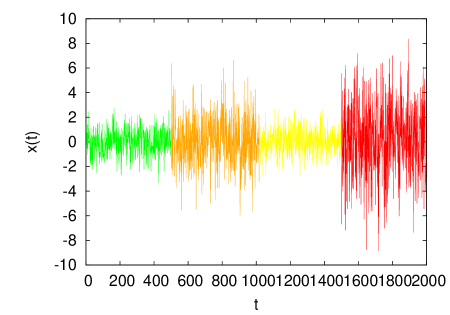
(a)

Figure 1: The time series consisting of 4 segments. Sequences in each segment are sampled from a zero-mean Gaussian distribution. The standard deviation is set as 1, 2, 1, and 3 from the left segment. The length of each segment is set as 500.

Table 1: The length, mean and standard deviation of each segment detected by the proposed method.

segment	start	end	length	mean	std. dev.
1	1	500	500	-0.00691	1.000
2	501	1017	517	0.0524	1.986
3	1018	1500	493	0.0320	0.980
4	1501	2000	500	0.212	2.929

4 Empirical analysis

1,413 companies listed on the first section of Tokyo Stock Exchange are selected for empirical analysis ($M=1,413$). The duration is 4th January 2000 to 30 January 2012. There are 2,675 business days during the observation period ($n=2,675$). These companies last during the observation period. I apply the recursive segmentation procedure to 1,413 security prices. I conducted the segmentation analysis of daily log-return time series between daily opening and ending prices defined in Eq. (1). Throughout the investigation $\Delta_{c}$ is fixed as 10 ($\alpha=0.99995$).

Fig. 2 shows the daily log return time series of Toyota Motor Corp (7203) segmented by using the proposed procedure. 9 segments are obtained in this case. The boundaries are computed in 2000-07-03, 2004-05-10, 2004-09-03, 2005-09-16, 2008-01-08, 2008-10-03, 2008-12-15, and 2009-04-16.

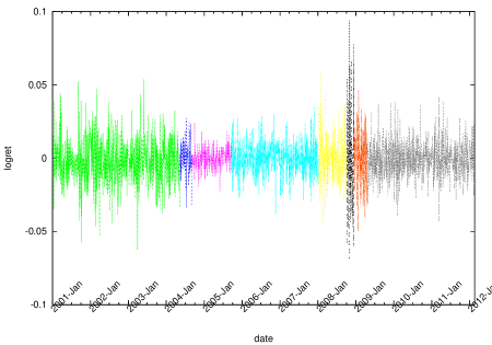
Figure 2: The daily log return time series of Toyota Motor Corp (7203) during the period from 4th January 2000 to 30th January 2012.

Fig. 3 shows the number of starting dates of segments for 1,413 log-return time series. The number of segments increase at (a) June 2000, (b) April 2004, (c) February 2006, and (d) 2007 to 2009. These seem to correspond to regimes or change points on Japanese economy. Specifically, during the latest global financial crisis the number of segments tend to increase (about 260 segments can be found at this period). Furthermore, after (e) 11 March 2011, the Great East Japan Earthquake, the number of segments steeply increased larger than the latest global financial crisis.

Figure 3: The number of staring dates of segments for 1,413 log-return time series during the period from 4th January 2000 to 30th January 2012.

The number of segments belonging to the same quintile of variances is counted. I computed order statistics of variance $\{\sigma_{i,(1)}\leq\ldots\leq\sigma_{i,(m_{i})}\}$ in $m_{i}$ segments of stock $i$. Next, each segment of stock $i$ is labeled $k=\{1,2,3,4,5\}$ depending on variance which belongs to the quintile. The number of segments which have the same labels is counted at each day. Fig. 4 shows the number of segments belonging to each quintile at every day. The number of first quintile segments shows stability of economic affairs, and the number of fifth quintile segments indicates instability of economic affairs. It is found that from 2003 to 2007 (I) the Japanese economy was in stable regime. From the end of 2007 (II) the unstable regime was observed. Specifically September 2008 (III), when we experienced the Lehman shock, the number of fifth quintile regimes steeply increased. This implies that the money flows of Japanese economy became unstable just after the Lehman shock. From March 2009 (IV) the money flow eventually recovered and the number of unstable regimes decreased and the number of stable segments eventually increased. From 11 March to 10 April 2011 (V), the number of unstable regimes steeply increased due to the Great East Japan Earthquake. However, after that the number of stable regimes rapidly increased and the Japanese macroeconomic affairs have been recovered eventually.

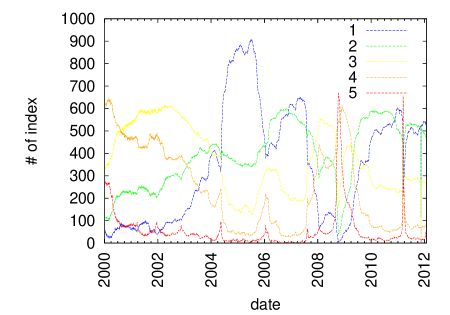
Figure 4: The number of segments in each quintiles for 1,413 log-return time series during 4th January 2000 to 30th January 2012.

Normally, we use only the past time series and want to foresee future macroeconomic conditions. To do so, at least the obtained results should be robust. In order to confirm the robustness, stability of the number of each regime, we consider two different time periods. We use two time periods for 2000-2010 (estimation) and for 2000-2012 (realization) and compare their results. The second is the same time series as ones shown in Fig. 4. Fig. 5 shows the number of regimes belonging to each quintile for two different periods. As seen from them it is confirmed that they are almost same until 2010. Namely, the time series may be employed to foresee future macroeconomic conditions.

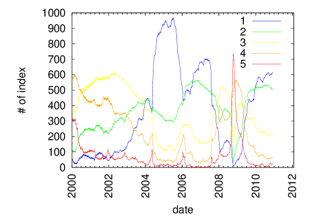
Figure 5: The number of segments in each quintiles for 1,413 log-return time series during 4th January 2000 to 14th December 2010.

5 Conclusion

A comprehensive time series segmentation analysis of the Japanese security prices was conducted. The daily log-returns for 1,413 security prices listed on the first section of the Tokyo Stock Exchange for 4 January 2000 to 14 December 2010 were analyzed by using a recursive segmentation procedure based on Jensen-Shannon divergence.

It was found that the number of segments increase at (a) June 2000, (b) April 2004, (c) February 2006, (d) 2007 to 2009, and (e) March 2011. These seemed to correspond to regimes or change points on Japanese economy.

The number of segments belonging to the same quintile of variances was counted. It was found that from 2003 to 2007 (I) the Japanese economy was in stable regime. From the end of 2007 (II) the unstable regime was observed. Specifically September 2008 (III), when we experienced the Lehman shock, the number of fifth quintile regimes steeply increased. This implies that the money flows of Japanese economy became unstable just after the Lehman shock. From March 2009 (IV) the money flow eventually recovered and the number of unstable regimes decreased and the number of stable segments eventually increased. After 11 March 2011 (V), the Great East Japan Earthquake, the number of segments steeply increased. From 11 March to 10 April 2011, the macroeconomic situations seemed to be negative, however, they were eventually recovered after that.

The volatility distribution computed from daily log-returns for a broad spectrum of stock prices traded in the Tokyo Stock Exchange market provides us with information on money flows at several economic levels. It may be further useful to understand the macroeconomic affairs of Japan in the quantitative way.

References

- (1) Mantegna, R.N. and Stanley, H.E.: An Introduction to Econophysics –Correlations and Complexity in Finance. Cambridge University Press, Cambridge (2000)
- (2) Bouchaud, J.P. and Potters, M.: Theory of Financial Risks and Derivative Pricing: From Statistical Physics to Risk Management, Cambridge University Press, Cambridge (2003)
- (3) Mandelbrot, B. : The Variation of Certain Speculative Prices, Journal of Business, 36, 394–419 (1963)
- (4) Gopikrishnan, P., Plerou, V. Liu, Y., L.A.N. Amaral, Gabaix, X, Stanley, H.E.: Scaling and correlation in financial time series, Physica A, 287, 362–373 (2000)
- (5) Praetz, P.D.: The Distribution of Share Price Changes. Journal of Business, 45, 49–55. (1972)
- (6) Gell-Mann, M. and Tsallis, C.: Nonextensive Entropy: Interdisciplinary Applications, Oxford University Press, New York (2004).
- (7) Sato, A.-H.: -Gaussian distributions and multiplicative stochastic processes for analysis of multiple financial time series. Journal of Physics: Conference Series, 201, 012008, 1–8 (2010)
- (8) Beck, C.: Dynamical Foundations of Nonextensive Statistical Mechanics, Physical Review Letters, 87 (2001) 180601.
- (9) Kozuki, N. and Fuchikami, N.: Dynamical model of financial markets: fluctuating ‘temperature’ causes intermittent behavior of price changes, Physica A, 329 (2003) 222–230
- (10) Ausloos, M. and Ivanova, K.: Dynamical model and nonextensive statistical mechanics of a market index on large time windows, Physical Review E, 68 (2003) 046122.
- (11) Beck, C.: Superstatistics: theory and applications, Continuum Mech. Thermodyn., 16 (2004) 293–304.
- (12) Goldfeld, S.M., and Quandt, R.E. : A Markov model for switching regressions. Journal of Econometrics, 1 (1973) 3–16.
- (13) S.A. Cheong, R.P. Fornia, G.H.T Lee, J.L. Kok, W.S. Yim, D.Y. Xu, and Y. Zhang: The Japanese Economy in Crises –A Time Series Segmentation Study, Economycs E-journal, 6 (2012) 2012-5, www.economics-ejournal.org.
- (14) Bernaola-Galván, P, Román-Roldán, R, and Oliver, J.L.: Gompositional segmentation and long-range fractal correlations in DNA sequences, Physical Review E, 53, 5181–5189 (1996)
- (15) Lin, J.: Divergence measures base on the Shannon entropy. IEEE Transactions on Information Theory, 37, 145–151 (1991)