A Theory of Quantum Observation and the Emergence of the Born Rule

Abstract

A realist description of our universe requires a twofold concept of locality. On one hand, there are the strictly Einstein-local interactions which generate the time evolution. On the other hand, the quantum state space calls for a non-local description of multi-particle states. This article uses a behavioristic approach to argue, that an observer in a universe like this has to rely on local interactions to learn about its properties and behavior. Such an observer is fundamentally restricted in his ability to understand and structurally reconstruct the individual local physical universe. We argue, that this reconstruction based on dynamically available information is the defining process of observation in quantum theory. The observer-centric view of the global quantum dynamics is shown to be non-unitary and non-linear in general, even if the universe itself evolves unitarily.

Interactions with massless free particles are found to have great influence on observation, because of their special role in the light-cone structure of an Einstein-local universe. For a specific scattering process with a photon of unknown state, the observed outcome can be subjectively random and follow the Born statistic, while the output state is really determined by the photon polarization. Based on this result, a theory of quantum measurement is formulated, which describes a measurement device as a cascade of scattering events.

I Introduction

Quantum theory is an enormously successful theory. We can use it to predict the behavior of nature very precisely up to the limits of measurement. This is even more astounding as we have almost no understanding of what “measuring” really means. Quantum theory equips us with an algorithm (Wallace2007, ) to describe, how the possible outcomes of a measurement can be calculated and predicted statistically. However, the measurement postulate of traditional quantum theory does not define, what a measurement instrument physically is, nor how it could possibly function. Even worse, it appears, that the process of measurement is not compatible with the smooth unitary evolution so fundamental to quantum theory.

A lot of effort has been placed into resolving this measurement problem and has resulted in a collection of interpretations of quantum theory (Schlosshauer2003, ; Wallace2007, ). Despite significant progress in some areas like decoherence theory, a generally accepted solution to the measurement problem is not currently known. From a realist perspective, one of the most important aspects of such a solution has to be a derivation of the statistical law of observations, the Born rule (Born1926, ), from fundamental properties of bare quantum theory. While such derivations have been attempted (Everett1957, ; SchlosshauerFine2005, ; Zurek2004, ; Zurek2007, ; Zurek2009, ), they usually involve non-obvious assumptions or have been shown to rely on circular or in other ways problematic arguments (Adler2003, ; Baker2006, ; Barnum1999, ; Dawid2013, ; Finkelstein2009, ; Hemmo2007, ; Jarlskog2011, ; Kent1990, ; Kent2009, ; Mohrhoff2004, ; Myrvold2005, ; Rae2008, ).

This article attempts to derive the discontinuous and random, yet stable results of observation as stated in the measurement postulate only from generally accepted first principles. This is done by assuming the position of an observer, who studies his environment in order to collect information about its behavior. Because the behavior is uniquely and completely determined by the well defined dynamics of the system, the result qualifies for a true realistic theory of quantum observation. That includes the possibility of experimental verification.

Everything we know about the universe is a result of our interaction with it, while being a part of it. As obvious as this statement may seem, it is of fundamental importance to our understanding of the way we describe the universe, create physical theories and interpret them. Even in the non-local setting of quantum theory, all interactions are subject to locality. In a relativistic universe, an observer is limited to his light cone and does not have access, in the form of interaction, to the complete state of the universe.

The idea of considering limited knowledge is not fundamentally new. The information available to the observer and the change of knowledge during measurement are also subject of the Copenhagen Interpretation, more precisely the quantum subjectivism proposed by Werner Heisenberg (Heisenberg1979, ). However, his idea has not evolved into a quantitative theory and it does not state the exact nature of the lack of knowledge.

Obtaining a quantitative characterization of the information available to the local observer corresponds to describing the state of the universe, that the observer would be able to reconstruct, based on its behavior, just from interaction without any additional assumptions.

To demonstrate the key idea, consider a simplified relativistic universe, containing just two (well localized) particles and an observer located close to one of these particles. The particles are supposed to have interacted a long time ago and are spatially well separated, to make sure that they cannot interact for another sufficiently long time. The observer, only being able to interact with one of the particles, is not in the position to tell if the two particles are entangled. In fact, he is unable to tell if a second particle exists at all. Based on the system’s behavior and not making unfounded assumptions, the observer’s description of the universe must not contain the other particle. The state he reconstructs, or assumes, if you will, is specifically not an improper mixed state, because that too would require knowledge about the existence of the other particle. He is left with the option of describing a single particle with a pure state, as we will discuss later in more detail.

A different, but similar, scenario is created by the interaction of the local system with free massless particles. Instead of a distant particle, imagine a photon, that has just been emitted into the environment. The information it carries is inaccessible as soon, as it leaves the observer’s horizon. Incoming photons also only become accessible the very instant, they reach the observer. The moment of interaction creates a discontinuity in the observer’s best guess for the state of the universe. The transport of information to and from the observer by interaction with the ambient radiation field also creates a source of randomness. The unknown state of the incoming radiation influences the local system in a way unpredictable to the local observer. The effect of the random perturbation is not entirely unpredictable however. It is restricted by the nature of the interaction, and shaped by the way the system couples to the radiation field. This opens the door for a statistical distribution, that correlates with the previously known state of the system, just like the Born distribution does. We will see, that the relevant no-go arguments are not applicable, because the linear structure of the state space is compromised by the local information constraint.

II The Postulates

In order to build the theory of local observation onto firm grounds, we use the following postulates. They formalize the assumptions used in the derivations presented and are well founded in what we already know about quantum theory. Most importantly, they do not introduce any new kind of structure.

1. The evolution of the state of the universe is unitary and generated only by interactions within the universe.

2. The interactions in the universe are local and in agreement with Special Relativity.

3. The observer mechanism is part of the universe, and its relevant parts are physically realized within a finite region of spacetime.

4. The description of the universe, as constructed by the observer, is based on his local state history, without any additional assumptions.

As observers, we do not have access to the state of the universe and a reduction of information from top to bottom might seem unnatural. We have to rely on Occam’s principle to argue, that a theory, which predicts local observations from an unknown global mechanisms, is valid, if the assumptions made on the global scale are very plain and simple. This is true for the postulates listed above and therefore supports the postulate of a global unitary evolution.

Postulate 4 not only restricts the description of the universe to the information processing happening in the observer system. It also defines, what we can regard to be physically distinguishable properties of the universe. Properties, that no imaginable observer can distinguish, cannot be part of the ontological description of the universe. It is only the dynamical sequence of the states of the universe—its behavior—, that results in an emergent physical reality.

In addition to these postulates, we still have to make one assumption about the universe to be able to derive the Born rule. That is the existence of a free massless neutral spin-1 boson field, that interacts with the observer. The photon takes this role in our universe.

The rest of this article uses these postulates to derive fundamental properties of all possible descriptions of the universe by an observer. There is no possible strategy, a local mechanism could follow to circumvent these properties. They are binding and must be taken into account when discussing the apprearance of the universe from an observer point of view.

III Local State Behavior

III.1 The state space of the universe

Our first postulate demands unitary evolution of the state of the universe, but it does not specify the state space. Instead, we will try to construct the state space from first principles.

The state space must be able to hold unitary representations of the observed symmetries of the universe. It must also be able to encode superposition and interference of states. These requirements are fulfilled by a complex vector space with a sesquilinear inner product, where the inner product allows unitary transforms to be defined. It is not entirely unreasonable to assume, that the state space is finite dimensional, but it is mathematically more convenient to allow for an infinite number of dimensions. In this case, the convergence of the inner product must be listed as an additional requirement. And we arrive at the well known separable Hilbert space $\mathcal{H}$ of square integrable functions.

Another possible state space, which meets all requirements, is the space of linear operators on the specified Hilbert space. We can embed the Hilbert space vectors as projectors within this larger space and inherit the inner product in the form of the trace of an operator product. Again, for an infinite dimensional state space this trace must exist. As such, one is limited to trace class linear operators.

The dynamic evolution of the universe acts in these state spaces with a time dependent unitary transform. The transform is one-sided for the Hilbert space and two-sided for the operator space. This is also true for all other unitary (symmetry) transforms.

$$\ket{\phi(t)} =U(t_{0},t)\ket{\phi(t_{0})}$$ (1)

$$\Phi(t) =U(t_{0},t)\Phi(t_{0})U(t_{0},t)^{\dagger}$$ (2)

Following postulate 4, only the sequence of states generated by the dynamical evolution is of physical relevance. As a result, state descriptions that are equivalent by a bijection $f$, which commutes with the evolution, are physically indistinguishable, because it allows switching back and forth between two representations at any point in time.

An important bijection is the left multiplication of $\Phi(t)$ with a unitary, possibly time dependent, but easily predictable operator, that commutes with the evolution of the universe. This operation can be undone at any point in time and satisfies the general equivalence condition

$$U(t_{0},t)f(\Phi)U^{\dagger}(t_{0},t) =f(U(t_{0},t)\Phi U^{\dagger}(t_{0},t))$$ (3)

with $f(\Phi):=S\Phi$ and $[S,U(t_{0},t)]=0$ for this case. So this $f(\Phi)$ is a redundant representation of $\Phi$. However, the redundancy does not correspond to an actual symmetry of the universe, because those symmetries act on both sides of the state representation. Therefore, these redundant states are not significant for the description of the universe and have to be removed for a unique state description. The subspace of Hermitian trace class operators does not allow for this one sided transform and using it for the state space gets rid of some of the redundant states. The non-negative Hermitian trace class operators $\mathcal{P}$ are even exactly the quotient of the trace class operators and equivalence by left (or right) unitary multiplication. Hence they are an even less redundant choice for the state space.

Both possible state spaces $\mathcal{H}$ and $\mathcal{P}$ can be reduced even further. The linear structure of the spaces allows for scalar multiplication as bijection that trivially commutes with the dynamics. The two equivalence relations

$$(\ket{a},\ket{b})\in R_{1} \Leftrightarrow\exists c\neq 0\in\mathbb{C}:\ket{a}=c\ket{b}$$ (4)

$$(A,B)\in R_{2} \Leftrightarrow\exists r>0:A=rB$$ (5)

generate the quotient spaces $\mathcal{H}/R_{1}$ and $\mathcal{P}/R_{2}$ of normalized states vectors in the Hilbert space $\mathcal{H}$ and the non-negative unit-trace Hermitian operator space $\mathcal{P}$ respectively.

The state space $\mathcal{P}/R_{2}$ is usually constructed as the space of “classical ensembles” of quantum systems, realized by the convex sum of projectors on the Hilbert space $\mathcal{H}$. It is also used to describe the state of subsystems by tracing over the environment. The first of these two uses relies strongly on the prior existence of the measurement postulate and cannot be used for our purpose. As for the second, tracing over the environment is not a possible operation when describing the whole universe. And tracing is not clearly motivated regarding the exact meaning of the result, apart from the compatibility with the measurement postulate. Here, the state space $\mathcal{P}/R_{2}$ was specifically constructed from basic requirements to show that it is a valid state space, just like the projective Hilbert space $\mathcal{H}/R_{1}$, without the need for an additional interpretation as space of ensembles or subsystem states. Any meaningful interpretation must naturally follow from the behavior of the state representation under the system evolution. This is an important insight for the arguments used further down.

We can apply postulate 4 again to group dynamically indistinguishable states, that describe the same physical behavior. Consider a state $\Phi(t_{0})\in\mathcal{P}$ and its evolution:

$$\Phi(t) =U(t_{0},t)\Phi U(t_{\text{0}},t)^{\dagger}$$ (6)

Then, with the unitarity of $U$ it follows, that

$$\Phi(t)^{2} =U(t_{0},t)\Phi(t_{0})U(t_{0},t)^{\dagger}U(t_{0},t)\Phi(t_{0})U(t_{0},t)^{\dagger}$$ (7)

$$=U(t_{0},t)\Phi(t_{0})^{2}U(t_{0},t)^{\dagger}$$ (8)

implying $\Phi^{2}$ evolves in exactly the same way as $\Phi$. At any point in time, we can switch back and forth between these two states, without making a difference dynamically, because squaring is a bijection on non-negative Hermitian operators and commutes with the evolution. The two states $\Phi$ and $\Phi^{2}$ are dynamically equivalent, and as such both describe the same physical system. The same holds true for all natural powers of a state $\Phi$, they too are bijections.

More generally, let

$$g\,:\,\mathbb{R}_{\geq 0} \longrightarrow\mathbb{R}_{\geq 0}$$ (9)

be an analytic bijection. Such a function is necessarily strictly monotonic and $g(0)=0$. It can be analytically extended to non-negative Hermitian operators and is a bijection there too. Any such $g$ creates a state, that is dynamically equivalent to the state it acts on. The equivalence classes generated by these bijections $g$ are again a better description of physical states.

One subset of the equivalence classes can be directly identified: The projectors in $\mathcal{P}$ are invariant under $g$, up to scalar multiplication, and each forms an equivalence class of its own. When $g$ acts on a state $\Phi$ it preserves two properties: The mutually orthogonal eigensubspaces are invariant. And the ordering of the eigenvalues is also strictly preserved, because $g$ is strictly increasing on the non-negative real numbers. The number of eigenvalues is countable because $\mathcal{H}$ is separable, and the trace-class bounds the sum of the non-negative eigenvalues, so that the maximum of the eigenvalues exists. It follows, that a possible representation of the equivalence classes of physical states then consists of a list of orthogonal eigensubspaces in order of decreasing eigenvalues, and nothing else. Particularly, the eigenvalues do not have to be specified, as they do change with $g$. For a finite list, the last entry is the nullspace, which is invariant under $g$. It is redundant, because it is the unique orthogonal complement of the direct sum of the other list entries. Therefore, this last entry may be omitted.

Depending on the equivalence class, the subspace list can have a different number of entries. For a simple projector it only has one entry, the eigensubspace with the maximum eigenvalue, which trivially equals 1. That is also the one property, that all equivalence classes share. All equivalence classes can be partially characterized with the eigensubspace of the greatest eigenvalue, which always exists.

Applying the unitary evolution of the universe to the eigensubspace lists shows, that the evolution acts independently on each subspace and does not change the dimensions of the subspaces or the length of the list. The character of the equivalence classes is therefore invariant under time evolution. This effectively splits up the state space into an infinite set of state spaces with common character and each connected by unitary transforms.

With all these considerations in place, the result is an infinite number of possible state spaces, that each allow for unitary evolution of the universe and do not encode the identified symmetries. Each state space is fully characterized by a finite list or infinite sequence of natural numbers or countable infinity, describing the dimensions of a the subspaces. The evolution acts unitarily on each subspace. For example, the original Hilbert space $\mathcal{H}$ is contained in the set of state spaces as the sequence $(\,1\,)$, representing a single one dimensional subspace, which the evolution acts on.

The n-dimensional projectors state space $(\,n\,)$ creates a physical universe that slightly differs from $\mathcal{H}$. One can decide to describe such a universe with a single vector from the eigensubspace and will get consistent dynamics. So the one dimensional state description is not unique, and even several different one dimensional descriptions could be used at the same time. This universe can be understood as a generated by $n$ non-interfering superpositions of orthogonal, but not uniquely determined $\mathcal{H}$ universes. Observers would notice the absence of interference in certain situations. But for finite $n$ that effect would be so rare that such a universe is practically indistinguishable from a $(\,1\,)$ universe. Furthermore a coincidence of eigenvalues to form a more than 1-dimensional eigensubspace is very unlikely, in fact those configurations form a subset of measure zero for all practical measures on the operator representation.

For universes with a state space with more than one relevant subspace $(\,n,\ldots\,)$, the description of their behavior can be simplified further. There must be, at least in principle, an experiment, that can distinguish different values of a quantity for it to be of physical relevance. This is equivalent to saying, the evolution must be able to produce different outcomes depending on that quantity. In the case of the unitary evolution we are discussing here, there is no way for the dynamics to depend on the number of subspaces in the state list. The number of subspaces is therefore not a feature of the state’s behavior. It is not physically relevant.

With the number of subspaces inherently unknown, the description of the individual subspaces also cannot be relevant. Consequently, there is not much left to be used for a state description. We know from deduction, that one subspace must always exist; the one with the greatest eigenvalue.

This can also be motivated by applying an explicit bijection

$$g_{k}(\Phi) =\Phi^{k}$$ (10)

for natural $k$ to a non-negative trace class Hermitian operator representation. For sufficiently large $k$, the largest eigenvalue dominates as strongly as desired. So the dynamics of the equivalence class representatives realized as a state operator can get arbitrarily close to the dynamics of the states in $(\,n\,)$. And for $k\to\infty$ we recover that space as the limit. As a result, there is no new physics to be expected in $(\,n,\ldots\,)$ universes compared to an $(\,n\,)$ universe, which is an accumulation point of the equivalence class.

It follows, that the map $g_{k}$ for $k\to\infty$, corresponding to the projection onto the eigensubspace with the largest eigenvalue, is a useful tool for reducing the complexity of the dynamical description in non-projection state space universes.

Summing up, the behavior of a unitarily evolving system is fully captured in a $(\,n\,)$ state description, which for $n=1$ is reduced to the traditional Hilbert space $\mathcal{H}$. This conclusion and the corresponding construction will be used further down to describe the behavior of the universe, as perceived by a local observer. There, additional constraints due to the light-cone structure of the universe will become relevant.

III.2 Local interactions and available state information

One of the most obvious weaknesses of the measurement postulate of traditional quantum theory lies in the lack of a precise definition of an observer. For our purpose, an observer must be a mechanism equipped with a memory and realized by physical interactions in the universe. It analyzes its environment, stores information and makes predictions based on these observations. This comes with the implicit emergence of a certain subjective reality for the observer, based on the behavior of the universe around him.

An observer of this kind can be human, but it does not have to be. The complexity and details of the mechanism are not of importance for the essential properties of our observer. Accordingly, these aspects will not be part of the model. The mere presence of an observer within the system will be assumed, even if the number of degrees of freedom is much too small to actually contain any sensible realization of such an observer mechanism. We will also assume, that there is a rest frame for the observer. A discussion of the precise nature of the observer-centric constraints follows.

III.2.1 Stripping the universe

In its rest frame, we can assume the relevant parts of the observer to be contained in a spherical spatial region of radius $r_{l}$. The universe outside of this radius is not part of the observer mechanism, but it does influence the observer by interaction up to a radius

$$r_{h}: =r_{l}+c\,T$$ (11)

limited by the observation time $T$ of the observer and the upper speed bound $c$ for the propagation of the effect of interactions. During the observation, this radius is a strict horizon for the information, the observer can recover about the universe. Anything outside the horizon is dynamically inaccessible and therefore not part of the local behavior and his experience of reality.

In a classical universe, we could simply remove all objects or fields on the far side of the horizon and the observer would not notice. The observer can only reconstruct the state of the universe as one without any structure outside the horizon, if he does not want to rely on arbitrary guesswork.

In principle, the same applies to a quantum universe, but with a non-trivial complication. Each particle carries its own copy of spatial information, instead of sharing one spatial background like in a classical universe. Starting with a single particle Hilbert space $\mathcal{H}_{1}$ and ignoring indistinguishability and different kinds of particles for now, we can define the $n$-particle space by taking the tensor product power

$$\mathcal{H}_{n}: =\mathcal{H}_{1}^{\otimes n}$$ (12)

and in the next step the Fock space of the particles as the direct sum of all possible $n$-particle spaces. The one dimensional vacuum space is denoted by $\mathcal{H}_{1}^{\otimes 0}$.

$$\mathcal{H}_{F} :=\bigoplus_{n=0}^{\infty}\mathcal{H}_{1}^{\otimes n}$$ (13)

For a single particle space, we can introduce two projection operators $P_{a}$ and $P_{i}$, that project onto the dynamically accessible and inaccessible states respectively. Naturally, $P_{a}+P_{i}=\mathbf{1}$ must hold. In case that accessibility is determined by the horizon with radius $r_{h}$ as defined above, we can explicitly express the projectors in the position basis of the single particle Hilbert space.

$$P_{a} :=\int_{r\leq r_{h}}\ket{\mathbf{r}}\bra{\mathbf{r}}d^{3}\mathbf{r}$$ (14)

$$P_{i} :=\int_{r>r_{h}}\ket{\mathbf{r}}\bra{\mathbf{r}}d^{3}\mathbf{r}$$ (15)

The eigensubspaces of both of these projectors, $\mathcal{H}_{a}$ and $\mathcal{H}_{i}$, hold the accessible and inaccessible states. We can write the single particle Hilbert space as a direct sum of these two orthogonal subspaces.

$$\mathcal{H}_{1}=\mathcal{H}_{a}\oplus\mathcal{H}_{i}$$ (16)

Expanding the Fock space definition with this substitution results in

$$\mathcal{H}_{F} =\mathcal{H}_{1}^{\otimes 0}\oplus\bigoplus_{n=1}^{\infty}\mathcal{H}_{a}^{\otimes n}\oplus\bigoplus_{n=1}^{\infty}\mathcal{H}_{i}^{\otimes n}$$ (17)

$$\oplus\bigoplus_{n,m=1}^{\infty}S\left(\mathcal{H}_{a}^{\otimes n},\mathcal{H}_{i}^{\otimes m}\right)$$

where $S\left(\mathcal{H}_{a}^{\otimes n},\mathcal{H}_{i}^{\otimes m}\right)$ is the symmetrized direct sum of the tensor product of $n$ times $\mathcal{H}_{a}$ and $m$ times $\mathcal{H}_{i}$. For example the symmetrization $S\left(\mathcal{H}_{a}^{\otimes 2},\mathcal{H}_{i}^{\otimes 1}\right)$ expands to:

$$S\left(\mathcal{H}_{a}^{\otimes 2},\mathcal{H}_{i}^{\otimes 1}\right)= \left(\mathcal{H}_{a}\otimes\mathcal{H}_{a}\otimes\mathcal{H}_{i}\right)$$

$$\oplus \left(\mathcal{H}_{a}\otimes\mathcal{H}_{i}\otimes\mathcal{H}_{a}\right)$$

$$\oplus \left(\mathcal{H}_{i}\otimes\mathcal{H}_{a}\otimes\mathcal{H}_{a}\right)$$ (18)

If we want to strip the inaccessible information from $\mathcal{H}_{F}$ in equation (17), we can first drop the pure $\mathcal{H}_{i}$ powers, similarly to the classical situation. The remaining inaccessible parts of the state space appear in tensor products with the accessible subspace. Removing these inaccessible parts, while keeping as much as possible of the accessible parts intact, will also remove relative phase information contained in the eliminated factor. This is in full agreement with the preservation of the local behavior. If we have two state components, that are orthogonal in the full state space, then they will not interfere. The reduction procedure may however map them to identical local states, which are still not allowed to interfere, because that is the behavior to be preserved.

So we cannot add the two states coherently. We would not know the relative phase anyway. The stripped state space must therefore contain a way to superimpose states without interference, while containing the Fock space $\mathcal{H}_{F}$.

The expanded state space for local reductions is given by the trace class non-negative hermitian operators on $\mathcal{H}_{F}$ denoted by $T(\mathcal{H}_{F})$, with the canonical embedding of the first as projections in the latter. The dynamics preserving map

$$S\left(\mathcal{H}_{a}^{\otimes n},\mathcal{H}_{i}^{\otimes m}\right) \to T\left(\mathcal{H}_{a}^{\otimes n}\right)$$ (19)

can then be realized by tracing over the inaccessible tensor factor spaces. This operation keeps the relative weights and eliminates all structural information in the inaccesible factor spaces without touching the accessible factor spaces.

Let $\ket{\Psi}$ be a Fock state and $\ket{\psi_{n}}$ its $n$-particle component.

$$\ket{\Psi} =\sum_{n=0}^{\infty}c_{n}\ket{\psi_{n}}$$ (20)

The projection operators $P_{a}^{(k,n)}$ and $P_{i}^{(k,n)}$ act on the $k$-th particle in the $n$-particle subspace. Stripping only the 1-particle subspace starts with distributing the projectors over the state.

$$\ket{\psi_{1}} =\left(P_{a}^{(1,1)}+P_{i}^{(1,1)}\right)\ket{\psi_{1}}$$ (21)

$$=P_{a}^{(1,1)}\ket{\psi_{1}}+P_{i}^{(1,1)}\ket{\psi_{1}}$$

If the particle is entirely accessible and therefore

$$P_{i}^{(1,1)}\ket{\psi_{1}} =0$$ (22)

we already have a stripped state. If the particle is entirely inaccessible we have

$$P_{a}^{(1,1)}\ket{\psi_{1}} =0$$ (23)

and dropping the inaccessible part would result in a physically undefined state, the $0$-vector. Instead, the observer should simply find no particle, or in other words, the vacuum state $\ket{\psi_{0}}$. The vacuum state can already be part of $\ket{\Psi}$ however, and the observed subjective vacuum must not interfere with the true vacuum. The two vacua must add incoherently. To simplify the notation we can identify the vacuum space $\mathcal{H}_{1}^{\otimes 0}$ with the complex scalars and choose:

$$\ket{\psi_{0}} =1\in\mathbb{C}$$ (24)

So if we apply the stripping map

$$\Lambda:\mathcal{H}_{F} \to T\left(\mathcal{H}_{F}\right)$$ (25)

to the vacuum and single particle subspaces we get

$$\Lambda\left(c_{0}\ket{\psi_{0}}+c_{1}\ket{\psi_{1}}\right)$$ (26)

$$=\Lambda\left(c_{0}\ket{\psi_{0}}+c_{1}P_{a}^{(1,1)}\ket{\psi_{1}}+c_{1}P_{i}^{(1,1)}\ket{\psi_{1}}\right)$$

$$=T\left(c_{0}\ket{\psi_{0}}+c_{1}P_{a}^{(1,1)}\ket{\psi_{1}}\right)+\mathrm{tr}_{\mathcal{H}_{1}}\left(T\left(c_{1}P_{i}^{(1,1)}\ket{\psi_{1}}\right)\right)$$

where

$$T\left(\ket{\phi}\right): =\ket{\phi}\bra{\phi}$$ (27)

is the natural embedding. The trace results in a complex number representing the vacuum state.

If we also consider two-particle states, we get additional terms from

$$\ket{\psi_{2}} =\left(P_{a}^{(1,2)}+P_{i}^{(1,2)}\right)\left(P_{a}^{(2,2)}+P_{i}^{(2,2)}\right)\ket{\psi_{2}}$$ (28)

$$=P_{a}^{(1,2)}P_{a}^{(2,2)}\ket{\psi_{2}}+P_{i}^{(1,2)}P_{i}^{(2,2)}\ket{\psi_{2}}$$

$$+P_{a}^{(1,2)}P_{i}^{(2,2)}\ket{\psi_{2}}+P_{i}^{(1,2)}P_{a}^{(2,2)}\ket{\psi_{2}}$$

The first term is not changed by $\Lambda$. The second term is mapped to the vacuum. And the last two terms are traced over to result in an incoherently mixing single particle state.

$$\Lambda\left(c_{0}\ket{\psi_{0}}+c_{1}\ket{\psi_{1}}+c_{2}\ket{\psi_{2}}\right)$$ (29)

$$=T\left(c_{0}\ket{\psi_{0}}+c_{1}P_{a}^{(1,1)}\ket{\psi_{1}}+c_{2}P_{a}^{(1,2)}P_{a}^{(2,2)}\ket{\psi_{2}}\right)$$

$$+\mathrm{tr}_{\mathcal{H}_{i}}\left(T\left(c_{1}P_{i}^{(1,1)}\ket{\psi_{1}}+c_{2}P_{a}^{(1,2)}P_{i}^{(2,2)}\ket{\psi_{2}}\right.\right.$$

$$\quad\left.\left.+c_{2}P_{i}^{(1,2)}P_{a}^{(2,2)}\ket{\psi_{2}}\right)\right)$$

$$+\mathrm{tr}_{\mathcal{H}_{i}^{\otimes 2}}\left(T\left(c_{2}P_{i}^{(1,2)}P_{i}^{(2,2)}\ket{\psi_{2}}\right)\right)$$

The trace is over all terms with a single inaccessible particle. The different position of the traced tensor factor space in each term is not problematic. Reordering the inaccessible spaces does not change the result, as they are traced over eventually. So we can think of that reordering implicitly happening while tracing.

As can be seen, this becomes tedious and complicated to write down for an increasing number of particle number eigenspace contributions. The definition of $\Lambda$ is a lot easier, if we express it in terms of an occupation number basis of $\mathcal{H}_{F}$, starting from a single particle eigenbasis of the projection operators $P_{a}$ and $P_{i}$ and assuming indistinguishable particles this time. With the bases $\ket{k}_{a}$ and $\ket{k}_{i}$ for $\mathcal{H}_{a}$ and $\mathcal{H}_{i}$ respectively and natural $k$, we can characterize a fully symmetric $n$-particle state by listing the number of particles $n_{k;a}$ and $n_{k;i}$ in each accessible and inaccessible single particle base state. The total particle number is then

$$n =\sum_{k=0}^{\infty}\left(n_{k;a}+n_{k;i}\right)$$ (30)

and we can label the state

$$\ket{\left(n_{0;a},n_{1;a},n_{2;a},\cdots\right);\left(n_{0;i},n_{1;i},n_{2;i},\cdots\right)}$$ (31)

or in a more compact form

$$\ket{\mathbf{n}_{a};\mathbf{n}_{i}}$$ (32)

with the occupation lists $\mathbf{n}_{a}$ and $\mathbf{n}_{i}$ respectively.

For our convenience we define

$$\left|\mathbf{n}_{a}\right|: =\sum_{k=0}^{\infty}n_{k;a}$$ (33)

and likewise for $\left|\mathbf{n}_{i}\right|$, so that:

$$n =\left|\mathbf{n}_{a}\right|+\left|\mathbf{n}_{i}\right|$$ (34)

With the occupation number basis of the Fock space, it can be seen from direct calculation, that $\ket{\mathbf{n}_{a};0}$ remains unchanged under $\Lambda$, while states with inaccessible single particle states are mapped to stripped states.

$$\ket{\mathbf{n}_{a};\mathbf{n}_{i}} \mapsto T\left(\ket{\mathbf{n}_{a};0}\right)$$ (35)

This already includes the case of all inaccessible states being mapped to the vacuum. The full stripping map is then defined for both bosonic and fermionic states and explicitly given by the following expression.

$$\Lambda\,:\,\mathcal{H}_{F} \longrightarrow T\left(\mathcal{H}_{F}\right)$$ (36)

$$\ket{\Psi} \longmapsto\Lambda\left(\ket{\Psi}\right)$$

$$\Lambda\left(\ket{\Psi}\right) :=\sum_{\mathbf{n}_{i}}T\left(\sum_{\mathbf{n}_{a}}\ket{\mathbf{n}_{a};0}\braket{\mathbf{n}_{a};\mathbf{n}_{i}}{\Psi}\right)$$

For an entirely accessible state we get

$$\Lambda\left(\ket{\Psi_{a}}\right) =\ket{\Psi_{a}}\bra{\Psi_{a}}$$ (37)

while fully inaccessible states are mapped to the vacuum.

$$\Lambda\left(\ket{\Psi_{i}}\right) =\ket{\circ}\bra{\circ}$$ (38)

The construction of the stripping map guarantees, that an observer interacting with the universe will not be able to distinguish the real state of the universe $\ket{\Psi}$ from the stripped state $\Lambda(\ket{\Psi})$. He certainly cannot construct a more accurate description of the universe than the stripped state. But does he even have the means to reconstruct the stripped state itself? The answer must be, that he cannot, for the following two reasons.

First, the classification of accessible and inaccessible states based on the horizon radius discussed above is not very precise. While all states marked as dynamically inaccessible are in fact certainly not accessible, not all states marked as accessible really are practically accessible. That means, the stripped state contains information, that is not available to the observer even under almost ideal conditions. We will discuss this in more depth below, when we look at the process of observing an experiment.

The second reason is the inability of the observer to distinguish state representations, that are equivalent under unitary evolution. The localized state description will not evolve unitarily in general, nonetheless unitarity is an important special case for which the reduction has to be applicable and consistent. Like discussed in section III.1, $\Lambda(\ket{\Psi})$ is, for example, intrinsically indistinguishable from its positive integer powers, if we assume unitary evolution. Consequently, the observer does not have enough information to reconstruct the stripped state without further assumptions about the state of the universe. As we have seen, the only assumption, that does not require the addition of arbitrarily made up information is, that the reconstructed state of the universe is a $(\,n\,)$ state. Following the earlier discussion about the state of the universe, we define the normalized stripped state in $\mathcal{H}_{F}$ as the normalized limit of the bijection (10).

$$\bar{\Lambda}:\mathcal{H}_{F}^{\prime} \longrightarrow\mathcal{H}_{F}$$ (39)

$$\ket{\Psi} \longmapsto T^{-1}\left(\bar{\Lambda}(\ket{\Psi})\right)$$

$$\bar{\Lambda}(\ket{\psi}) :=\lim_{k\to\infty}\frac{\Lambda(\ket{\Psi})^{k}}{\mathrm{tr}\left(\Lambda(\ket{\Psi})^{k}\right)}$$

The limit is a projection operator onto the eigensubspace of $\Lambda(\ket{\Psi})$ with the greatest eigenvalue. For a so called pure state, the eigensubspace must be one dimensional, which can then be naturally mapped back to the Hilbert space $\mathcal{H}_{F}$ by $T^{-1}$. If we assume, that the eigenvalues are essentially random, then it is extremely unlikely, that eigenvalues become exactly equal and form an eigensubspace with dimension greater than one. So it seems to be safe to assume, that $\bar{\Lambda}(\ket{\Psi})$ practically always results in a pure state. The states that do not get mapped back to a pure state are formally removed from $\mathcal{H}_{F}^{\prime}$. We will see, that the time evolution of the resulting state becomes essentially non-linear once we drop the unitarity assumption for the stripped state evolution.

III.2.2 Making an observation

The process of observation is based on interactions and limited by their finite propagation speed in a relativistic universe. Hence, the reconstructed state refers to a time slice in the past of the observer. This time asymmetry is created by the requirement of a memory to consolidate the state information. The implied arrow of time does not affect the measurement process at this point and reconstructing a future state leads to the same fundamental properties. We will see, that the process itself will allow for an independent time arrow to be inherited from the radiation field.

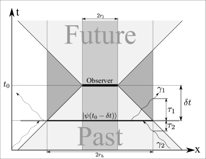
Figure 1: The observer reconstructs the state $\ket{\psi}$ based on the information collected from past interactions. The photons $\gamma_{1}$ and $\gamma_{2}$ transport information to and from the environment beyond the observation horizon.

Figure 1 shows the situation in spacetime. The observer with radius $r_{l}$ reconstructs the state $\ket{\psi(t_{0}-\delta t)}$ at the time $t_{0}$ from information in his past light cone. The observation delay $\delta t$ and the radius of the reconstructed state horizon are related by $r_{h}=r_{l}+c\,\delta t$. During an observation the delay is held constant, so that the observed system evolves on the same time base as the observer. Anything outside the world volume swept by the space inside the horizon is not part of the observer’s subjective reality.

In a typical experimental setup, the observer focuses on a more or less isolated object at relative rest. It is a reasonable simplification to assume, that the only exchange of information with the unobserved universe is due to electromagnetic interactions. The two photons shown on the left do not have any effect on the reconstructed reality of the observer, because their interaction is constrained to the spatial region outside the reconstruction horizon. This is not true for the photons $\gamma_{1}$ and $\gamma_{2}$. They do interact with the reconstructed state. The corresponding durations of the interaction with the world volume of the state are $\tau_{1}$ and $\tau_{2}$. During that time, the state reconstruction performed by the observer will change in a non-unitary way. Furthermore, the observer will not be able to directly reconstruct the existence of either photon, because it does not pass through his own world volume.

As discussed before, the reconstructed state is described by a single Hilbert space vector. The outgoing and incoming photons are of unknown polarization state, which leads to a random element being introduced to the reconstructed state. The change of the state happens on the same , almost instant, time scale as the typical interaction with a photon. The reconstructed subjective state description will therefore change suddenly and non-unitarily to a random outcome state. This is not only in agreement with the measurement postulate. At this point it seems natural to conjecture a relationship between the interaction with photons and what is called quantum measurement. The next chapter discusses the relevant process in more detail.

IV Simple interactions between Radiation and Matter

Let us consider a system consisting of only a single qubit. There is nothing else, the observer can use to compare the qubit to. Not even the observer itself exists as part of the quantum system in this simple model. The qubit is the entire observable universe, and we can apply the reconstruction procedure to it.

Nonetheless, the qubit is not completely insulated, as we assume it couples to the radiation field. The interaction is described by a unitary evolution on the entire unobserved universe. To keep it simple, the only states of the radiation field, that are considered, are inaccessible. The incoming state can be thought of as a single photon with a 2-dimensional representation of its polarization. The outgoing states can more complicated than that, depending on the scattering process, and we do not specifically keep track of polarization. We call these scattering processes elementary, because only two qubits, one for the photon and one local to the observer, are given as the input state.

We will discuss three canonical cases of elementary scattering processes explicitly. In all of them, the state of the local qubit is represented in the orthonormal basis $\{\ket{0},\ket{1}\}$, which is chosen to coincide with the physically preferred basis for the resulting process. The incoming photon state will be written as a linear combination of the orthonormal basis states $\{\ket{\leftrightarrow},\ket{\updownarrow}\}$. For the outgoing radiation states an arbitrary orthonormal basis $\{\ket{\rightsquigarrow_{n}}\,:\,n\in\mathbb{N}\}$ is used. The vacuum state is $\ket{\circ}$. All processes are unitary, because they map orthonormal states in the input space to orthonormal states in the output space.

The input state corresponds to the objective state of the universe just before the interaction. And the output state is the objective state just after the interaction. Both, input and output radiation states are locally inaccessible and will be removed in the local state reconstruction, so that we can study the scattering process as observed locally. The state of the photon is considered to be entirely unknown. We will write the photon component of the input state to the left of the qubit component and for the output state to the right of the qubit, only to indicate the incoming and outgoing radiation and without any deeper mathematical or physical meaning.

The general input state in this setup is

$$\ket{\psi} :=\left(\alpha\ket{\updownarrow}+\beta\ket{\leftrightarrow}\right)\left(a\ket{0}+b\ket{1}\right)$$ (40)

$$=\alpha a\ket{\updownarrow}\ket{0}+\alpha b\ket{\updownarrow}\ket{1}$$

$$+\beta a\ket{\leftrightarrow}\ket{0}+\beta b\ket{\leftrightarrow}\ket{1}$$ (41)

for $\alpha,\beta,a,b\,\in\mathbb{C}$ with the non-vanishing condition:

$$\alpha\alpha^{*}+\beta\beta^{*} >0$$ (42)

$$aa^{*}+bb^{*} >0$$ (43)

The local reconstruction of the input $\ket{\psi}$ is then simply

$$\bar{\Lambda}(\ket{\psi}) =T((a\ket{0}+b\ket{0})\ket{\circ})$$ (44)

which is equivalent to the local qubit state, just like one would expect.

IV.1 The uniform elementary scattering process

Consider the following unitary mapping of the input space basis to the output space basis:

$$U_{u}\,:\, \left.\begin{array}[]{r}\ket{\updownarrow}\ket{\text{0}}\\ \ket{\updownarrow}\ket{1}\\ \ket{\leftrightarrow}\ket{0}\\ \ket{\leftrightarrow}\ket{1}\end{array}\right\}\longmapsto\left\{\begin{array}[]{l}\ket{0}\ket{\rightsquigarrow_{1}}\\ \ket{0}\ket{\rightsquigarrow_{2}}\\ \ket{1}\ket{\rightsquigarrow_{3}}\\ \ket{1}\ket{\rightsquigarrow_{4}}\end{array}\right.$$ (53)

The objective input state $\ket{\psi}$ is then mapped to

$$U_{u}\ket{\psi} =\alpha a\ket{0}\ket{\rightsquigarrow_{1}}+\alpha b\ket{0}\ket{\rightsquigarrow_{2}}$$ (54)

$$+\beta a\ket{1}\ket{\rightsquigarrow_{3}}+\beta b\ket{1}\ket{\rightsquigarrow_{4}}$$

The stripped local state of the output is then

$$\Lambda(U_{u}\ket{\psi}) =T\left(\alpha a\ket{0}\ket{\circ}\right)+T\left(\alpha b\ket{0}\ket{\circ}\right)$$ (55)

$$+T\left(\beta a\ket{1}\ket{\circ}\right)+T\left(\beta b\ket{1}\ket{\circ}\right)$$

$$=\alpha\alpha^{*}(aa^{*}+bb^{*})\ket{0}\bra{0}\ket{\circ}\bra{\circ}$$ (56)

$$+\beta\beta^{*}(aa^{*}+bb^{*})\ket{1}\bra{1}\ket{\circ}\bra{\circ}$$

After taking the projection limit and mapping the result into the Hilbert space, we get

$$\bar{\Lambda}(U_{u}\ket{\psi}) =\begin{cases}\ket{0}\ket{\circ}&\text{if}\;\alpha\alpha^{*}>\beta\beta^{*}\\ \ket{1}\ket{\circ}&\text{if}\;\alpha\alpha^{*}<\beta\beta^{*}\end{cases}$$ (57)

The state of the photon is entirely unknown and we can assume that any polarization state has the same probability. Then the symmetry of the result allows the deduction of the probabilities of either outcome and we find both to be equally likely. The case of exact equality of $\alpha\alpha^{*}$ and $\beta\beta^{*}$ is of zero measure and can be ignored in the statistics.

Summarizing, we have a process $U$ that acts locally like

$$U_{u}\,:\,a\ket{0}+b\ket{1} \mapsto\begin{cases}\ket{0}&\text{with probability}\,p_{\text{0}}=\frac{1}{2}\\ \ket{1}&\text{with probability}\,p_{1}=\frac{1}{2}\end{cases}$$ (58)

Notably, the result does not depend on the state of the local input qubit. A local observer just sees a fully random outcome that can be predicted only in terms of probabilities, while the global process is entirely deterministic. The missing information about the exact photon state creates the illusion of a spontaneous random change of the local quantum state.

IV.2 The maximum elementary scattering process

After having seen a process whose result only depends on the photon state, the existence of a process with only local qubit dependence is not very surprising. A small, yet significant, modification of the unitary map generates such a scattering result: outcome:

$$U_{m}\,:\, \left.\begin{array}[]{r}\ket{\updownarrow}\ket{\text{0}}\\ \ket{\updownarrow}\ket{1}\\ \ket{\leftrightarrow}\ket{0}\\ \ket{\leftrightarrow}\ket{1}\end{array}\right\}\longmapsto\left\{\begin{array}[]{l}\ket{0}\ket{\rightsquigarrow_{1}}\\ \ket{1}\ket{\rightsquigarrow_{2}}\\ \ket{0}\ket{\rightsquigarrow_{3}}\\ \ket{1}\ket{\rightsquigarrow_{4}}\end{array}\right.$$ (67)

The objective input state $\ket{\psi}$ is mapped to

$$U_{m}\ket{\psi} =\alpha a\ket{0}\ket{\rightsquigarrow_{1}}+\alpha b\ket{1}\ket{\rightsquigarrow_{2}}$$ (68)

$$+\beta a\ket{0}\ket{\rightsquigarrow_{3}}+\beta b\ket{1}\ket{\rightsquigarrow_{4}}$$

which is stripped and results in

$$\Lambda(U_{m}\ket{\psi}) =T\left(\alpha a\ket{0}\ket{\circ}\right)+T\left(\alpha b\ket{1}\ket{\circ}\right)$$ (69)

$$+T\left(\beta a\ket{0}\ket{\circ}\right)+T\left(\beta b\ket{1}\ket{\circ}\right)$$

$$=aa^{*}(\alpha\alpha^{*}+\beta\beta^{*})\ket{0}\bra{0}\ket{\circ}\bra{\circ}$$ (70)

$$+bb^{*}(\alpha\alpha^{*}+\beta\beta^{*})\ket{1}\bra{1}\ket{\circ}\bra{\circ}$$

Eventually, with the limit and the Hilbert space map in place we arrive at

$$\bar{\Lambda}(U_{m}\ket{\psi}) =\begin{cases}\ket{0}\ket{\circ}&\text{for}\,aa^{*}>bb^{*}\\ \ket{1}\ket{\circ}&\text{for}\,aa^{*}<bb^{*}\end{cases}$$ (71)

So in total we get the local observation of the form

$$U_{m}\,:\,a\ket{0}+b\ket{1} \mapsto\begin{cases}\ket{0}&\text{if}\;|a|>|b|\\ \ket{1}&\text{if}\;|b|>|a|\end{cases}$$ (72)

The unknown photon state does not influence the outcome. And the process is fully deterministic, even for a local observer. The result is a perceived projection onto the dominant component of the qubit in the preferred basis.

IV.3 The Born rule generating elementary scattering process

The two scattering processes discussed above only use information from either the qubit or the photon state to determine the local output. Next, we will discuss a process that mixes the influence of both equally and results in a statistical rule that also depends on the state of the qubit. The map, that creates this behavior is

$$U_{B}\,:\, \left.\begin{array}[]{r}\ket{\updownarrow}\ket{\text{0}}\\ \ket{\updownarrow}\ket{1}\\ \ket{\leftrightarrow}\ket{0}\\ \ket{\leftrightarrow}\ket{1}\end{array}\right\}\longmapsto\left\{\begin{array}[]{l}\ket{0}\ket{\rightsquigarrow_{1}}\\ \left(\ket{1}\ket{\rightsquigarrow_{2}}+\ket{0}\ket{\rightsquigarrow_{3}}\right)/\sqrt{2}\\ \left(\ket{0}\ket{\rightsquigarrow_{4}}+\ket{1}\ket{\rightsquigarrow_{5}}\right)/\sqrt{2}\\ \ket{1}\ket{\rightsquigarrow_{6}}\end{array}\right.$$ (81)

and produces the output state

$$U_{B}\ket{\psi} =\alpha a\ket{0}\ket{\rightsquigarrow_{1}}+\beta b\ket{1}\ket{\rightsquigarrow_{6}}$$ (82)

$$+\alpha b\left(\ket{1}\ket{\rightsquigarrow_{2}}+\ket{0}\ket{\rightsquigarrow_{3}}\right)/\sqrt{2}$$

$$+\beta a\left(\ket{0}\ket{\rightsquigarrow_{4}}+\ket{1}\ket{\rightsquigarrow_{5}}\right)/\sqrt{2}$$

which strips to

$$\Lambda(U_{B}\ket{\psi})=T\left(\alpha a\ket{0}\ket{\circ}\right)\\ +\frac{1}{2}\left(T\left(\alpha b\ket{1}\ket{\circ}\right)+T\left(\alpha b\ket{0}\ket{\circ}\right)\right)\\ +\frac{1}{2}\left(T\left(\beta a\ket{0}\ket{\circ}\right)+T\left(\text{$\beta$a}\ket{1}\ket{\circ}\right)\right)\\ +T\left(\beta b\ket{1}\ket{\circ}\right)\\ =\left(\alpha\alpha^{*}aa^{*}+\frac{1}{2}\left(\alpha\alpha^{*}bb^{*}+\beta\beta^{*}aa^{*}\right)\right)\ket{0}\bra{0}\ket{\circ}\bra{\circ}\\ +\left(\beta\beta^{*}bb^{*}+\frac{1}{2}\left(\alpha\alpha^{*}bb^{*}+\beta\beta^{*}aa^{*}\right)\right)\ket{1}\bra{1}\ket{\circ}\bra{\circ}$$ (83)

and after mapping the result to pure states we get:

$$\bar{\Lambda}(U_{B}\ket{\psi}) =\begin{cases}\ket{0}\ket{\circ}&\text{if}\;\alpha\alpha^{*}aa^{*}>\beta\beta^{*}bb^{*}\\ \ket{1}\ket{\circ}&\text{if}\;\alpha\alpha^{*}aa^{*}<\beta\beta^{*}bb^{*}\end{cases}$$ (84)

The outcome of the scattering process depends on both, the amplitudes of the qubit in the preferred basis and the unknown incoming photon state.

We do not have any information about the state of the photon, but we know that it is in a state that is fully described by $\alpha$ and $\beta$. Total ignorance implies that the statistical distribution of $\alpha$ and $\beta$ does not depend on the choice of a basis, or in other words, the distribution of $(\alpha,\beta)$ must be invariant under $SU(2)$ transforms.

One possible distribution that realizes this symmetry is given by

$$\alpha :=G_{1}+iG_{2}$$ (85)

$$\beta :=G_{3}+iG_{4}$$ (86)

Where $G_{n}$ are mutually independent identically distributed Gaussian random variables with zero mean. Because the sum of two independent Gaussian variables results in a new Gaussian variable, this construction is invariant under unitary transformations. This guarantees $SU(2)$ uniformity of the distribution. The case $\alpha=\beta=0$ leads to an invalid state, but is of zero measure, so we can safely ignore it. The magnitude of a complex gaussian random variable is Rayleigh distributed, so that we have

$$|\alpha| =R_{1}$$ (87)

$$|\beta| =R_{2}$$ (88)

with two equally distributed, but independent Rayleigh variables $R_{1}$ and $R_{2}$. The probability density function of each is:

$$f(x) =x\exp(-\frac{x^{2}}{2})$$ (89)

The probability $p\left(|a|\,|\alpha|>|b|\,|\beta|\right)$ can be expressed in terms of this probability density function:

$$p\left(|a|\,|\alpha|>|b|\,|\beta|\right) =\int_{0}^{\infty}\int_{0}^{\frac{|a|}{|b|}x_{1}}f(x_{1})f(x_{2})dx_{2}dx_{1}$$ (90)

$$=\frac{|a|^{2}}{|a|^{2}+|b|^{2}}$$ (91)

And of course, for the complementary event we find:

$$p\left(|a|\,|\alpha|<|b|\,|\beta|\right) =\frac{|b|^{2}}{|a|^{2}+|b|^{2}}$$ (92)

The local observation is therefore

$$U_{B}\,:\,a\ket{0}+b\ket{1} \mapsto\begin{cases}\ket{0}&\text{with }\,p_{\text{0}}=\frac{|a|^{2}}{|a|^{2}+|b|^{2}}\\ \\ \ket{1}&\text{with }\,p_{1}=\frac{|b|^{2}}{|a|^{2}+|b|^{2}}\end{cases}$$ (93)

which constitutes the Born rule.

This process realizes two key aspects of the measurement postulate. The outcome locally appears to be a pure state, randomly selected from a preffered set of orthogonal states. And the probability of seeing a specific outcome is proportional to the squared magnitude amplitude of the possible outcome states.

We do not yet have the entire measurement postulate however. A complete derivation must deal with robustness under repeated “measurements” and systems larger than a single qubit. The next section will resolve these two remaining issues.

V Local Quantum Reality

V.1 Emergent reality and disrupted time

In the previous section we have been able to demonstrate the emergence of the Born rule from the local reconstruction of the behavior of an evolving global state. The analysis of the scattering processes has been restricted to a single qubit in an otherwise unpopulated observer regime and an initially pure quantum state.

Unfortunately, after a single scattering pass the state will not be subjectively pure anymore, but instead consist of two branches, encoded by the eigenvectors of the reduced state. A second pass will again map to the only two possible local output branches and the eigenvalues will mix between the two previous branches. We cannot expect the Born rule to hold under these conditions. And it turns out, that it does not in general.

A minor modification to the local system takes care of this problem and also makes our assumptions more realistic. An observer, who wants to test for the validity of the Born rule, has to be able to compare sequential observation results. Consequently, he has to have access to a recorded history of events. Adding a memory device to the local state of the observer makes the different outcomes of branches belonging to different iterations distinguishable and keeps them from mixing. The number of branches therefore doubles with each recorded qubit scattering process.

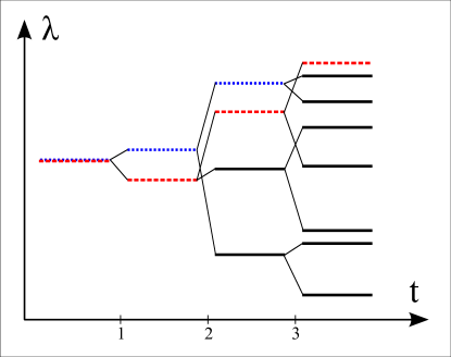
Figure 2: Evolution of the branches and their eigenvalues under Born scattering. The scattering events occur at times 1, 2 and 3. They result in new branches containing the records of the previous history the respective branch. The dotted blue lines show the dominant branch and its history after the first and second scattering events. One event later the red dashed line becomes the dominant branch with its own history. The single initial branch is part of both histories.

Figure 2 shows a sequence of Born scattering processes and the resulting change of the reconstructable branch, which the local observer is aware of. Looking only at the sequence of dominant branches, one can verify that the Born rule holds for the transitions 1 and 2, because the new dominant branch is created from the previous dominant branch. The situation is identical to the elementary scattering event with a single branch initial state. That does not hold true for the third scattering process. The formerly suppressed branch splits into the new dominant branch. Depending on the actual states, this sequence of branches usually breaks the Born rule.

Despite the partly compromised Born rule for the sequence of reconstructed states, the observer will never see any results, that are in disagreement with the Born rule. The reason for this lies in the way the observer tests the statistics of the results. He keeps a list of old results to compare to the new ones, and the branch switch not only determines the current observed result, but also the list of remembered states. This is also illustrated in figure 2. After the third branch switch, the observer remembers the history marked with the dashed red line. And this history describes a sequence of observation outcomes, which is in agreement with the Born rule.

Everything, that the observer would consider as part of his reality is contained in the current reconstructed state of the universe and his memory. We can therefore call the sequence of branches, which leads to the current reconstructed branch and that is stored in the memory of the observer an emergent subjective reality. A branch switch will not only change the current perception, but also the perception of history leading up to this state. The observer can switch between realities without even noticing, because all records will agree with the newly formed reality. This picture leaves subjective time and history disrupted by observed scattering events. This is a drastic, but seemingly unavoidable consequence of observation. A rough estimation of probabilities however stongly suggests, that an event, which uncovers a long time hidden reality branch is extremely unlikely. So the observer’s subjective history is stable after only a few scattering events.

V.2 Macroscopic interactions and quantum measurement

The three elementary scattering processes with the locally perceived non-unitary outcome as described here all act on single qubit systems. While their mechanisms are very similar, Born scattering comes with the unique property of scalability to macroscopic systems, as we will discuss now.

Consider a set of projectors

$$\mathbb{P} =\{P_{n}\,:\,n\text{$\in\mathbb{N}$}\}$$ (94)

acting on the Hilbert space $\mathcal{H}_{P}$ with the constraint, that all their commutators vanish:

$$[P_{m},P_{n}] =0$$ (95)

We also define the identity operator $\mathbb{I}_{P}$ on $\mathcal{H}_{P}$ and the complementary projectors

$$\bar{P}_{n} =\mathbb{I}_{P}-P_{n}$$ (96)

We call this set of projectors complete, if there is a special orthonormal basis $\{\ket{k_{P}}\}$ of $\mathcal{H}_{P}$ and we can find two (disjoint) sets $I_{1}(k),I_{2}(k)\subset\mathbb{N}$, so that

$$\ket{k_{P}}\bra{k_{P}} =\prod_{n\in I_{1}(k)}P_{n}\prod_{m\in I_{2}(k)}\bar{P}_{m}$$ (97)

for all $k$. The set is independent, if we cannot remove any projectors from $\mathbb{P}$ without giving up completeness.

With the set of projectors, there is a natural way to define a unitary evolution to split up vectors in $\mathcal{H}_{P}$.

$$U_{n} : \ket{\psi} \longmapsto P_{n}\ket{\psi}\otimes\ket{0}+\bar{P}_{n}\ket{\psi}\otimes\ket{1}$$ (98)

Here, $\{\ket{0},\ket{1}\}$ is the basis of a qubit and we can apply the Born scattering evolution to it, with the local result

$$\bar{\Lambda}(U_{B}U_{n}\ket{\psi})= \begin{cases}P_{n}\ket{\psi}\ket{0}&\text{with }p=\frac{\braket{\psi}{P_{n}}{\psi}}{\braket{\psi}{\psi}}\\ \\ \bar{P}_{n}\ket{\psi}\ket{1}&\text{with }p=\frac{\braket{\psi}{\bar{P}_{n}}{\psi}}{\braket{\psi}{\psi}}\end{cases}$$ (99)

We have seen, that the recorded subjective observation of qubits is consistent and stable, allowing us to restrict our discussion to the dominant branch and taking the position of the local observer. Repeating the observation with a different projector $P_{m}$ and a fresh qubit maps the first branch to $P_{m}P_{n}\ket{\psi}\ket{0}\ket{0}$ with the old qubit state as the last factor. For a cleaner notation, we write the qubit state ordered list inside a single ket $\ket{0,0}$. The probability of finding this branch combines the probabilities from both scattering events and results in:

$$p =\frac{\braket{\psi}{P_{n}^{\dagger}P_{m}^{\dagger}P_{m}P_{n}}{\psi}}{\braket{\psi}{P_{n}}{\psi}}\cdot\frac{\braket{\psi}{P_{n}}{\psi}}{\braket{\psi}{\psi}}$$ (100)

$$=\frac{\braket{\psi}{P_{m}P_{n}}{\psi}}{\braket{\psi}{\psi}}$$ (101)

As can be seen from generalizing this calculation, further scatterings only result in adding more projectors to the numerator of the probability expression. The order is arbitrary, because the projectors commute by definition. This is also true for the projectors in front of the state $\ket{\psi}$. We can therefore choose the canonical ordering of the index without changing the properties of the result, as far as they relate to the state $\ket{\psi}$. The order of the qubit history will change however. This motivates the definition of the operator

$$M =\prod_{n=1}^{N}U_{B}U_{n}$$ (102)

where each factor comes with a fresh qubit. We also define $\ket{[j]}$ as the qubit list with the $N$-digit binary expansion of $j$. Similarly, we define $P_{[j]}$ to be the product sequence with the digits $\{P_{n},\bar{P}_{n}\}$ following the $N$-digit binary representation of $j$.

The subjective local result of the application of $M$ on the state $\ket{\psi}$ is then:

$$\bar{\Lambda}(M\ket{\psi}) =\begin{cases}P_{[0]}\ket{\psi}\ket{[0]}&\text{with }p=\frac{\braket{\psi}{P_{[0]}}{\psi}}{\braket{\psi}{\psi}}\\ P_{[1]}\ket{\psi}\ket{[1]}&\text{with }p=\frac{\braket{\psi}{P_{[1]}}{\psi}}{\braket{\psi}{\psi}}\\ \vdots&\vdots\\ P_{[2^{N}-2]}\ket{\psi}\ket{[2^{N}-2]}&\text{with }p=\frac{\braket{\psi}{P_{[2^{N}-2]}}{\psi}}{\braket{\psi}{\psi}}\\ P_{[2^{N}-1]}\ket{\psi}\ket{[2^{N}-1]}&\text{with }p=\frac{\braket{\psi}{P_{[2^{N}-1]}}{\psi}}{\braket{\psi}{\psi}}\end{cases}$$ (103)

We are interested in the limit of very large $N$. In this case, the $P_{[k]}$ contain all possible projector lists as sublists. For a given list of projections, that multiplies to a projector on a single dimensional subspace, we can find a unique binary sequence, which produces this list as a sublist and preserves that subspace in the remaining projectors, because either $P$ or $\bar{P}$ preserves the subspace. All other lists containing the same sublist must multiply to $0$.

The consequence is, if we have a complete set of projectors $\mathbb{P}$, then there is exactly one outcome with non-zero probability resulting in the state $\ket{k_{P}}\otimes\ket{[j]}$, with a probability of

$$p =\frac{\braket{\psi}{k_{P}}\braket{k_{P}}{\psi}}{\braket{\psi}{\psi}}$$ (104)

Summarized, for complete $\mathbb{P}$ and sufficiently large $N$, the scattering iteration

$$\bar{\Lambda}(M\ket{\psi}) =\ket{k_{P}}\otimes\ket{[j]} p=\frac{\left|\braket{k_{P}}{\psi}\right|^{2}}{\braket{\psi}{\psi}}$$ with (105)

results in the Born rule for measurement in the basis $\{\ket{k_{P}}\}.$

We have constructed a measurement mechanism, that works for measured Hilbert spaces of arbitrary size and can therefore be applied to macroscopic systems. The mechanism does not need very special initial condition or careful tuning. In fact, it is very robust, as the order of the elementary scattering processes does not change the outcome, nor does the actual choice of projectors. A physical device realizing this mechanism should not be hard to design and build, given the single qubit scattering process can be realized.

So far, we only discussed the case of a complete set of projectors. The framework presented allows for generalizations, that are not discussed here however. It is interesting to note, that the Born rule is the only rule, which delivers robust and consistent results for a macroscopic system built from single qubit interactions, mostly due to the canceling terms in equation (100).

V.3 Realizing Born scattering on a qubit

The Born scattering process presented in the last section is very generic and does not refer to a specific physical system. As an example of a simple system, that can realize the scattering process, we will discuss the interaction between a single electron bound inside an atom and its interaction with the electromagnetic radiation field. We are looking at a transition of the electron, that happens between two energy levels and also changes the angular momentum. For example, in terms of the standard hydrogen quantum numbers, the states could be $\ket{n=1,l=0}$ and $\ket{n=2,l=1}$. For a simpler notation, we use the qubit notation $\ket{0}$ and $\ket{1}$ respectively.

With the angular momentum eigenstates for the qubit, the incoming single photon is best described in terms of a circular polarization basis $\ket{\rightsquigarrow\circlearrowleft}$ and $\ket{\rightsquigarrow\circlearrowright}$. The arrow to the right merely indicates the direction of the photon trajectory towards the atom prior to the collision.

If the incoming photon carries the wrong angular momentum for the transition, then nothing happens:

$$\ket{\rightsquigarrow\circlearrowleft}\ket{0}\mapsto\ket{0}\ket{\rightsquigarrow\circlearrowleft}$$ (106)

The photon with the opposite angular momentum can either be absorbed while exciting the electron, or shake the system a little and radiate away in a different direction. We assign the same amplitude to both options. The relative phase between them is irrelevant, it cancels in the reduction process.

$$\ket{\rightsquigarrow\circlearrowright}\ket{0}\mapsto\left(\ket{1}\ket{\circ}+\ket{0}\ket{\leftrightsquigarrow\circlearrowright}\right)\frac{1}{\sqrt{2}}$$ (107)

Here, $\ket{\circ}$ is the relative 0-photon state and $\ket{\leftrightsquigarrow}$ is the state of the scattered photon, which is orthogonal to the unchanged outgoing photon state.

Trying to add another angular momentum quantum to the already excited state also has to leave the system unchanged:

$$\ket{\rightsquigarrow\circlearrowright}\ket{1}\mapsto\ket{1}\ket{\rightsquigarrow\circlearrowright}$$ (108)

However, if we take the angular momentum of the excited state back by sending in and oppositely polarized photon, we can again have two possible effects. The incoming photon can either trigger the emission of a second photon with the same properties. Or the incoming photon only shakes the atom slightly and leaves in a new direciton. As above, the amplitudes of both processes are assumed to be equal while relative phase is not of importance.

$$\ket{\rightsquigarrow\circlearrowleft}\ket{1}\mapsto\left(\ket{0}\ket{\rightsquigarrow\circlearrowleft,\rightsquigarrow\circlearrowleft}+\ket{1}\ket{\leftrightsquigarrow\circlearrowleft}\right)\frac{1}{\sqrt{2}}$$ (109)

These four maps between an orthonormal basis of the input space and an orthogonal basis of a significantly different output space together describe a unitary evolution, that matches all the criteria, we have identified earlier for generating the Born rule for a local observer.

If it can be shown, that the equal amplitude assumption for the scattering outcome states is in agreement with light-matter interaction theory, then we should expect to find this mechanism everywhere around us.

VI Conclusion

We have presented a possible solution to the quantum measurement problem, that does not require any modification of the dynamics or state space of traditional quantum theory. Nor does it demand conditions for classicality or a specific kind of observer. The results are derived solely from a realist understanding of the state of the universe and the assumption, that identically behaving systems are in fact physically identical.

One of the main results is, that any internal description of the quantum universe leads to a non-linear model of the state of the universe and its evolution. This description can change discontinuously upon the interaction with ambient photons. We have seen, that, under certain conditions, the projective and random outcome, as described by the measurement postulate, emerges naturally. The corresponding mechanism and its consequences are within reach of experimental verification.

The derived measurement process nicely generalizes to arbitrarily large systems. A POVM (Audretsch2007, ) description of measurements is also covered, in the form of projective measurements on larger spaces. Furthermore, we have given a generalization of the concept of a quantum subsystem (Neumann1927, ), that does no longer have to be a tensor-factor space of the state space.

The derived results are compatible with relativistic quantum theory. In fact, they require a relativistic universe to be deducible. At the same time, the physicality of the nonlocality of the quantum state space is revealed, that is normally hidden under the inderterminism of observations. The underlying breach of Lorentzian symmetry might become experimentally accessible, if deterministic control of measurement outcomes can be physically realized.

The key idea of physical behaviorism does not play a relevant role in any main stream interpretation of quantum theory. While this fact alone makes it stand out, there are still many more fundamental differences. A great advantage is, that the locally perceived pure state of the universe is very robust and well defined, unlike in theories, that exclusively rely on entanglement to define features of histories, events and relationships. Examples for these interpretations include MWI (Everett1957, ; DeWitt1973, ), consistent histories (Dowker1996, ; Griffiths1984, ; Okon2013, ), but also bare decoherence (Zeh1993, ; Zurek2002, ; Schlosshauer2007, ; Joos2003, ) and decoherent histories (Bassi1998, ).

Everett’s relative state interpretation takes the idea of subjective reality very far. Not only does every observer experience his own reality, each observer also splits up into a vast number of copies, who also experience all possible histories (Everett1957, ). The theory we present here leads to a much more restricted notion of subjective reality. A single observer’s perception of reality is greatly restricted by what he does not know about the universe. That is foremostly the state of incoming or outgoing photons. Two observers at roughly the same position in spacetime will share practically all of their ignorance about these states and therefore come to the same conclusions about their local reality. By extension and covering a whole time-slice with observers, that have spatially overlapping descriptions of their immediate past, we can deduce the existence of a single connected subjective reality. There is only one “world”. And it specifically does not depend on the strategy of the observer to deal with it. Still, we do share the branching structure with MWI and we have seen, that, on a short time scale, many different realities can be realized, but one at a time. Only a single one of those realities does have a realized future in the long run, but all do have a full recorded history reaching into the past.

Ontologically, the given theory of quantum measurement is very attractive. It combines the objective realism of the universal quantum state with subjective features of one’s own description of this state. All postulates are harmless, from a philosophical point of view, and they represent well established physics. The notion of an all-creating dynamical law reduces the ontological requirements of the theory to the absolute minimum. It also allows to avoid fuzzy concepts, like improper mixtures for the description of what we know about quantum states.

One mostly philosophical problem does emerge however. The concept of linear time as a reference for events in reality cannot be maintained from the global perspective of the subjective reality. Undetectable to the observer, different alternate realities can fight for becoming the dominant one, at least over a short period of time. This effect appears to be highly unsettling and not really greatly preferable to the world-splitting in the Everett interpretation. Currently, and with the evidence presented here, there does not seem to be a way around it. Further research will have to analyze this in more depth and may offer alternatives.

The local observation theory uniquely features a physical mechanism with an objective source of randomness. That means unlike MWI, no additional probability structure is needed for us to be able to consistently speak about the frequency of observed events. Also unlike Bohmian mechanics (Bell1982, ; Bell2004, ), there are no fragile initial conditions to be met in order to recover the Born statistic.

A certain detail in the derivation Born rule needs some further attention. The assumption of equal amplitude magnitudes for the two concurring scattering processes is not obviously true. The symmetry of the choice and the existence of certain conservation laws seem to favor the equality, but it is by no means guaranteed to hold. This is an area, which will need more investigation and a better model. The predictive power of this choice is nevertheless so great, that the assumption can be just justified for now. This is particularly true with the Born rule being the only statistical process, that survives macroscopification, bringing in the aspect of natural selection for observable processes.

The proposed solution significantly differs in all relevant aspects from the established interpretations of quantum theory and is at the same time experimentally accessible. Even more, it has the potential to make the nonlocal nature of quantum theory directly available for experiments. The possibility of controlling subjectively indeterministic processes by manipulation of the underlying scattering processes could greatly extend the tool set of quantum manipulations and forces us to rethink established results, that rely on the fundamentality of randomness in quantum observations or linearity.

- [1] Stephen L. Adler. Why decoherence has not solved the measurement problem: a response to P.W. Anderson. Studies In History and Philosophy of Science Part B: Studies In History and Philosophy of Modern Physics, 34(1):135–142, March 2003.
- [2] G.C. Ghirardi Angelo Bassi. Decoherent histories and realism. Journal of statistical physics, pages 457–494, 1998.
- [3] Jürgen Audretsch. Entangled Systems: New Directions in Quantum Physics. Wiley-VCH, 2007.
- [4] N. Graham B. DeWitt, editor. The many-worlds interpretation of quantum mechanics. Princeton University Press, 1973.
- [5] David Baker. Measurement outcomes and probability in everettian quantum mechanics. Studies In History and Philosophy of Science Part B, 38(1):153–169, May 2007.
- [6] H. Barnum, C. M. Caves, J. Finkelstein, C. A. Fuchs, and R. Schack. Quantum probability from decision theory? Proc. R. Soc. Lond. A, 456:1175–1182, 2000.
- [7] J. S. Bell. Speakable and Unspeakable in Quantum Mechanics: Collected Papers on Quantum Philosophy. Cambridge University Press, 2. edition, June 2004.
- [8] John Stewart Bell. On the impossible pilot wave. Found. Phys., 12:989–999, Jun 1982.
- [9] Max Born. Zur Quantenmechanik der Stoßvorgänge. Zeitschrift für Physik, 37(12):863–867, December 1926.
- [10] Richard Dawid and Karim P Y Thebault. Against the empirical viability of the deutsch wallace approach to quantum mechanics. Preprint: http://philsci-archive.pitt.edu/9541/, January 2013.
- [11] Fay Dowker and Adrian Kent. On the consistent histories approach to quantum mechanics. Journal of Statistical Physics, 82(5):1575–1646, 1996.
- [12] C. Kiefer D. Giulini I.O. Stametescu E. Joos, H.D. Zeh. Decoherence and the Appearance of a Classical World in Quantum Theory. Berlin: Springer, 2nd edition, 2003.
- [13] Hugh Everett. Relative state formulation of quantum mechanics. Reviews of Modern Physics, 29:454–462, 1957.
- [14] J. Finkelstein. Has the born rule been proven? arXiv:0907.2064 [quant-ph], 2009.
- [15] G. C. Ghirardi, A. Rimini, and T. Weber. Unified dynamics for microscopic and macroscopic systems. Phys. Rev. D, 34:470–491, Jul 1986.
- [16] Robert B. Griffiths. Consistent histories and the interpretation of quantum mechanics. Journal of Statistical Physics, 36(1):219–272, 1984.
- [17] Werner Heisenberg. Quantentheorie und Philosophie. Reclam, 1979.
- [18] Meir Hemmo and Itamar Pitowsky. Quantum probability and many worlds. Studies in History and Philosophy of Science Part B, 38(2):333–350, 2007.
- [19] Cecilia Jarlskog. A comment on a recent derivation of the born rule by zurek. arXiv:1107.3736 [quant-ph], 2011.
- [20] A. Kent. Against many-worlds interpretations. International Journal of Theoretical Physics, A5:1745, 1990.
- [21] A. Kent. One world versus many: The inadequacy of everettian accounts of evolution, probability, and scientific confirmation. arXiv: quant-ph/0905.0624, 2009.
- [22] Arthur Fine Maximillian Schlosshauer. On Zurek’s derivation of the Born rule. Foundations of Physics, 35(2), February 2003.
- [23] Ulrich Mohrhoff. Probabilities from envariance? International Journal of Quantum Information, 2(2):221–230, 2004.
- [24] W. C. Myrvold. Why I am not an Everettian. Unpublished manuscript. http://users.ox.ac.uk/~everett/docs/Myrvold%20Not%20an%20Everettian.pdf.
- [25] Elias Okon and Daniel Sudarsky. On the consistency of the consistent histories approach to quantum mechanics. arXiv:1301.2586 [gr-qc], January 2013.
- [26] Alastair I. M. Rae. Everett and the Born rule. Studies In History and Philosophy of Science Part B, 40(3):243–250, 2009.
- [27] Maximilian Schlosshauer. Decoherence, the measurement problem and interpretations of quantum mechanics. arxiv: quant-ph/0312059, 2003.
- [28] Maximilian A. Schlosshauer. Decoherence and the Quantum-To-Classical Transition. Springer, April 2008.
- [29] John von Neumann. Wahrscheinlichkeitstheoretischer Aufbau der Quantenmechanik. Nachr. Ges. Wiss. Göttingen, pages 245–272, 1927.
- [30] David Wallace. The quantum measurement problem: State of play. arXiv:0712.0149v1 [quant-ph], 2007.
- [31] W. K. Wootters and W. H. Zurek. A single quantum cannot be cloned. Nature, 299(5886):802–803, 1982.
- [32] H.D. Zeh. There are no quantum jumps, nor are there particles! Physics Letters A172, page 189, 1993.
- [33] W. H. Zurek. Decoherence and the transition from quantum to classical—revisited. Los Alamos Science, 27:2–25, 2002.
- [34] W. H. Zurek. Probabilities from entanglement, Born’s rule from envariance. arXiv:quant-ph/0405161v2, 2004.
- [35] W. H. Zurek. Quantum darwinism. Nature Physics, 5:181–188, 2009.
- [36] Wojciech H. Zurek. Relative states and the environment: Einselection, envariance, quantum darwinism, and the existential interpretation. arXiv:0707.2832 [quant-ph], 2007.