Force-extension relation of cross-linked anisotropic polymer networks

Abstract

Cross-linked polymer networks with orientational order constitute a wide class of soft materials and are relevant to biological systems (e.g., F-actin bundles). We analytically study the nonlinear force-extension relation of an array of parallel-aligned, strongly stretched semiflexible polymers with random cross-links. In the strong stretching limit, the effect of the cross-links is purely entropic, independent of the bending rigidity of the chains. Cross-links enhance the differential stretching stiffness of the bundle. For hard cross-links, the cross-link contribution to the force-extension relation scales inversely proportional to the force. Its dependence on the cross-link density, close to the gelation transition, is the same as that of the shear modulus. The qualitative behavior is captured by a toy model of two chains with a single cross-link in the middle.

I Introduction

Anisotropic networks are abundant in nature and among man-made materials. For example, nematic elastomers WT or actin-myosin assemblies in cells Cooper . These networks are constructed from anisotropic building blocks, nematogens such as stiff rods or semiflexible polymers which are well modelled by wormlike chains (WLCs) STY . Isotropic networks of WLCs have been studied extensively in experiment Kroy_Bausch , driven by the interest in biological networks such as the cytoskeleton or the extracellular matrix. Theoretical approaches have dealt with entangled solution Morse as well as chemically cross-linked networks of WLCs Head ; Wilhelm . The former build on the tube model whereas the latter generalise concepts from rubber elasticity. Aligning linkers can give rise to a variety of morphologies which have been studied by means of a generalised Onsager approach Borukhov as well as within a microscopic model BZ ; Kiemes . Of particular interest are bundles of filaments which occur in a broad range of cytosceletal structures and show much richer elastic behaviour than the usual WLC Claessens ; Lieleg ; Heussinger . Two parallel-aligned, stretched semiflexible filaments cross-linked by a motor cluster have been used as the minimal elastic element of an active gel MCM .

Here, we consider an anisotropic network of WLCs which have been aligned along a preferred axis chosen as the $z$–direction. The alignment is not due to cross-links which we model as springs. Instead possible mechanisms for alignment are a nematic environment, pulling forces, grafting surfaces or the Onsager mechanism. A sketch of such a network is shown in Fig. 1. If the alignment is strong, the WLC model can be replaced by a weakly bending chain (WBC) as first suggested by Marco and Siggia MS for DNA molecules. The advantage for an analytical approach is enormous because the single chain model is Gaussian. Our focus in this paper lies on the force-extension curve of a randomly cross-linked anisotropic network of strongly aligned filaments. We first consider a toy model, consisting of two cross-linked filaments. The model allows us to disentangle the contributions to the effective extension which are due to either bending stiffnes or cross-links. Subsequently, we analyse the effects of cross-links for a macroscopic network.

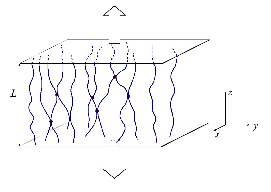
Figure 1: network of aligned wormlike chains under pulling force

II Model

Our starting point is the energy of a stretched WLC in terms of the tangent vector ${\bf t}(s)=\frac{d{\bf r}(s)}{ds}=(\frac{d{\bf r}_{\perp}}{ds},\frac{dz}{ds})\;$,

$${\cal H}[{\bf t}(s)]=\frac{\kappa}{2}\int_{0}^{L}ds\Big{(}\frac{d{\bf t}(s)}{ds}\Big{)}^{2}-f\int_{0}^{L}ds\frac{dz}{ds}\;.$$ (1)

Here $\kappa$ denotes the bending stiffnes which is related to the persistence length $L_{p}$ via $L_{p}=2\kappa/((d-1)k_{B}T)$, where $d$ is the dimensionality of the embedding space. The pulling force is denoted by $f$, and $0\leq s\leq L$ is the arclength. The local inextensibility constraint of the WLC is expressed by the condition $|{\bf t}(s)|=1$. We assume that the chain is strongly stretched so that tilting of the tangent vector away from the $z$–axis is small and we can use the approximation

$$\frac{dz}{ds}=\sqrt{1-\Big{(}\frac{d{\bf r}_{\perp}}{ds}\Big{)}^{2}}\approx 1-\frac{1}{2}\Big{(}\frac{d{\bf r}_{\perp}}{ds}\Big{)}^{2}$$ (2)

leading to the weakly bending model introduced by Marco and Siggia MS

$${\cal H}_{0}[{\bf r}_{\perp}(s)]=\frac{\kappa}{2}\int_{0}^{L}ds\Big{(}\frac{d^{2}{\bf r}_{\perp}(s)}{ds^{2}}\Big{)}^{2}+\frac{f}{2}\int_{0}^{L}ds\Big{(}\frac{d{\bf r}_{\perp}(s)}{ds}\Big{)}^{2}$$ (3)

The central quantity of interest is the extension of the chain under an applied force $f$, which in the weakly bending approximation is computed from the thermal fluctuations transverse to the aligning direction:

$$\langle z(L)-z(0)\rangle = \int_{0}^{L}ds{\Big{\langle}}\frac{dz}{ds}{\Big{\rangle}}$$ (4)

$$= \int_{0}^{L}ds{\Big{(}}1-{\Big{\langle}}\frac{1}{2}{\Big{(}}\frac{d{\bf r}_{\perp}}{ds}{\Big{)}}^{2}{\Big{\rangle}}{\Big{)}}$$

III Toy model: 2 cross-linked chains

Before addressing the full problem of a randomly cross-linked array of aligned chains, we discuss the much simpler case of two strongly stretched chains in two dimensions with one cross-link in the middle, see Fig. 2.

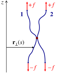
Figure 2: Two aligned chains with one cross-link in the middle

In two dimensions, ${\bf r}_{\perp}(s)=y(s)$ and the Hamiltonian reads

$${\cal H}={\cal H}_{0}[y_{1}(s)]+{\cal H}_{0}[y_{1}(s)]+\frac{g}{2}\Big{(}y_{1}({L}/{2})-y_{2}({L}/{2})\Big{)}^{2}$$ (5)

The cross-link is modeled as a harmonic spring of stiffness $g$. For simplicity we impose hinged-hinged boundary conditions: $y_{1}(0)=y_{1}(L)=0,\;y_{2}(0)=y_{2}(L)=D$ and $y^{\prime\prime}_{1}(0)=y^{\prime\prime}_{1}(L)=0,\;y^{\prime\prime}_{2}(0)=y^{\prime\prime}_{2}(L)=0$ for the two chains which are a distance $D$ apart (the prime denotes derivative with respect to $s$). According to the boundary conditions that we use, the eigenfunction representation should be

$$y_{1}(s)=\sum_{l=1}^{\infty}A_{l}\sin(q_{l}s)$$

$$y_{2}(s)-D=\sum_{l=1}^{\infty}B_{l}\sin(q_{l}s)$$

and wavenumbers are restricted to values $q_{l}=\frac{\pi}{L}l\;$, $l\in\mathbb{Z}$. These eigenfunctions diagonalise the Hamiltonian of the weakly bending chain, whereas the cross-link gives rise to a term which is quadratic in the amplitudes but not diagonal. Introducing vectors

$$\Gamma = (A_{1},B_{1},A_{2},...)\;,$$

$$u = g^{1/2}(\sin(q_{1}L/2),\;-\sin(q_{1}L/2),\;\sin(q_{2}L/2),...)$$

and matrices

$$C=\frac{L}{2}\begin{pmatrix}q_{1}^{2}(\kappa q_{1}^{2}+f)&0&0&\ldots\\ 0&q_{1}^{2}(\kappa q_{1}^{2}+f)&0&\ldots\\ 0&0&q_{2}^{2}(\kappa q_{1}^{2}+f)&\ldots\\ \vdots&\vdots&\vdots&\ddots\end{pmatrix}$$

the Hamiltonian is rewritten as

$$H=\frac{1}{2}\sum_{l,m=1}^{\infty}\Gamma_{l}G_{l,m}\Gamma_{m}+Dg^{1/2}\sum_{l=1}^{\infty}u_{l}\Gamma_{l}$$ (6)

with $G_{l,m}=C_{l,m}+u_{l}u_{m}.$ The matrix $G$ is easily inverted:

$$G^{-1}=C^{-1}-\frac{C^{-1}uu^{T}C^{-1}}{1+u^{T}C^{-1}u}\;,$$ (7)

so that we can compute the force-extension curve, say of chain 1, exactly

$$\langle z_{1}(L)\rangle\;=\;L-\frac{L}{4}\sum_{l}q_{l}^{2}\langle A_{l}^{2}\rangle\;.$$ (8)

Our model has three characteristic energies: the bending energy, $\kappa/L$, the work done by the external force, $fL$ and the thermal energy, $T$ (we set $k_{B}\equiv 1$). Use of the weakly bending approximation requires $\kappa/L\gg T$ (which is equivalent to $L_{p}/L\gg 1$) or $fL\gg T$. This leaves us with one free parameter, $x:=fL/(\kappa/L)$, namely the ratio of work done by the external force to bending energy. This dimensionless quantity can also be interpreted as the squared ratio of two lengthscales: the total contour length $L$ to the length $\sqrt{\kappa/f}$ over which the boundary conditions penetrate into the bulk (i.e., the size of a link in an effective freely-jointed chain) PBET . Actually, we have two additional lengthscales, the distance between chains, $D$, which we assume to be negligible and the length of the cross-link ($\propto 1/{\sqrt{g}})$ or alternatively the energy of a cross-link relative to the work done by the pulling force, $gL/f$.

The result for general $x$ and cross-link strength $g$

$$\frac{\langle z_{1}\rangle}{L}-1\;=\;-\Delta_{MS}-\Delta_{XL}$$ (9)

can be decomposed into a contribution, $\Delta_{MS}$, which is characteristic for a weakly bending chain and well-known from the work of Marko and Siggia MS and a contribution due to the cross-link, $\Delta_{XL}$

$$\Delta_{XL} = -\frac{gT}{16f^{2}}\frac{u_{2}(x)}{u_{0}(x)}$$

$$u_{0}(x) = \sqrt{x}+\frac{gL}{2f}\Big{(}\sqrt{x}-2\tanh(\sqrt{x}/2)\Big{)}$$

$$u_{2}(x) = 2\sqrt{x}+\sqrt{x}/(\cosh({\sqrt{x}/2}))^{2}-6\tanh(\sqrt{x}/2)$$

In the limit of large $x$, the cross-link contribution is given by

$$\Delta_{XL}=-\frac{gT}{8f^{2}}\left(1+\frac{gL}{2f}\right)^{-1}.$$ (10)

For soft cross-links $\Delta_{XL}$ falls off as $f^{-2}$, whereas in the limit of hard cross-links, $gL/f\to\infty$, we find $\Delta_{XL}=-T/(4fL)$. In any case, the contribution of the cross-link is subdominant in the limit of strong pulling force. Note that $\Delta_{XL}$ is independent of $\kappa$, which shows us that the contribution from the cross-link is purely entropic. This contribution could in fact be evaluated from a directed polymer model which does not involve any bending rigidity.

Collecting the leading terms for hard cross-links and strong pulling force, yields

$$\frac{\langle z_{1}\rangle}{L}-1\;=\;-\frac{T}{(4\kappa f)^{1/2}}-\frac{T}{4fL}-\frac{D^{2}}{8L^{2}}.$$ (11)

Here we have restored the term due to a finite distance, $D$, between the chains, which gives rise to a geometric reduction in length due to the cross-link. This term is presumably unimportant in a network, where $D/L$ is expected to be small. This term will be neglected in the following.

The weakly bending approximation is satisfied as long as the r.h.s. of Eq. (9) is small. We point out that, in the case of $L_{p}\gg L$, this approximation is fulfilled even without having very large $x$ (strong stretching). We show the relative extension as a function of pulling force in Fig. 3 for hard cross-links. As discussed, cross-linking enhances the extension due to the reduction of thermal fluctuations, but the effect becomes less and less pronounced in the strong stretching limit. It is also of interest to consider a situation, where a strong pulling force has been applied and subsequently the change in extension in response to a small change in the pulling force is measured. This response is determined by the differential stiffness ${df}/d\langle z_{1}\rangle$. In Fig. 4 we show the inverse stiffness for the same set of parameters as in Fig. 3

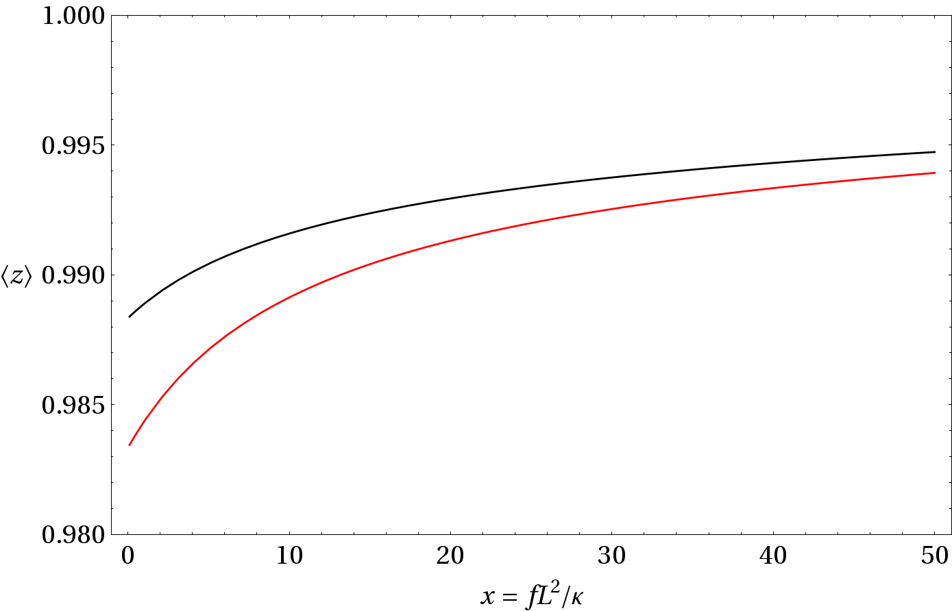
Figure 3: Force-extension curve for $L/L_{p}=1$; red (black) curve without (with) cross-link

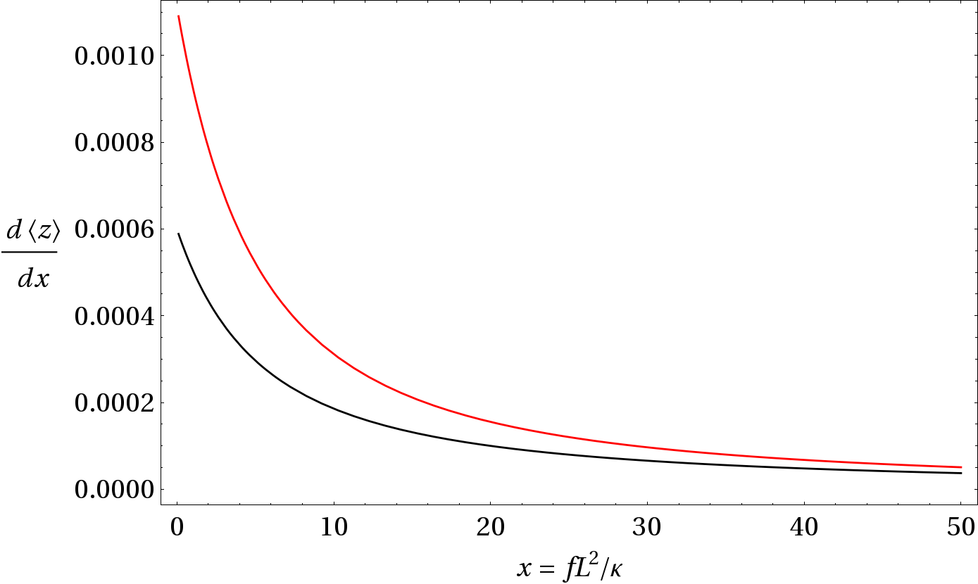
Figure 4: Inverse differential stiffnes for $L/L_{p}=1$; red (black) curve without (with) cross-link

As expected the cross-link enhances the differential stiffness. If the chains are already strongly stretched, the cross-link has little effect. However for weakly stretched chains the enhancement is considerable.

IV Randomly cross-linked network

In this Section, we are going to compute the force-extension relation of a randomly cross-linked ensemble of oriented chains approximately. We are guided by the result for the cross-linked pair of chains, which consists of a single chain contribution, $\sim T/(\kappa f)^{1/2}$, and a contribution due to the cross-link, $\sim T/(fL)$, which is independent of the bending rigidity $\kappa$. We decompose the calculation for the network accordingly: In the uncross-linked network, the force-extension relation is determined by the single chain contribution. To assess the effect of cross-linking, we compute the free energy difference of the cross-linked network relative to the uncross-linked system.

Our starting point is the Hamiltonian

$${\cal H}=\sum_{i=1}^{N}{\cal H}_{0}[{\bf r}_{i}(s)]+{\cal H}_{\text{ev}}+{\cal H}_{\text{Xlink}}(\mathcal{C}_{M})$$ (12)

with ${\cal H}_{0}$ given in Eq. (3). To simplify the notation, we have dropped the subscript ${\bf r}^{i}_{\perp}(s)\to{\bf r}_{i}(s)$, such that ${\bf r}_{i}$ denotes the transverse excursion of chain $i$. The excluded volume interaction

$${\cal H}_{\text{ev}}=\sum_{i<j}\frac{\lambda}{2}\int_{0}^{L}ds\,\delta\big{(}{\bf r}_{i}(s)-{\bf r}_{j}(s)\big{)}$$ (13)

is introduced to balance the attractive interactions due to cross-linking. The latter are modelled by harmonic springs

$${\cal H}_{\text{Xlink}}(\mathcal{C}_{M})=\frac{g}{2}\sum_{e=1}^{M}\big{(}{\bf r}_{i_{e}}(s_{e})-{\bf r}_{j_{e}}(s_{e})\big{)}^{2}.$$ (14)

where $\mathcal{C}_{M}:=\{i_{e},j_{e};s_{e}\}$ is a quenched configuration of $M$ cross-links connecting polymers $i_{e},j_{e}$ at arclength $s_{e}$.

The partition function of the cross-linked system relative to the uncross-linked melt for a specific realization of cross-links, $\mathcal{C}_{M}$, reads

$$Z(\mathcal{C}_{M})=\left\langle\exp\!\left(-\frac{{\cal H}_{\text{Xlink}}(\mathcal{C}_{M})}{T}\right)\right\rangle.$$ (15)

Here $\langle...\rangle$ denotes the thermal average over all polymer configurations with the Boltzmann weight $\exp(-{\cal H^{\prime}}/T)$ of the uncross-linked melt ${\cal H^{\prime}}=\sum_{i=1}^{N}{\cal H}_{0}[{\bf r}_{i}(s)]+{\cal H}_{\text{ev}}$.

Physical observables can be calculated from the quenched-disorder averaged free energy, $\Delta F=-T[\ln Z]$, where $[...]$ denotes average over all realizations of random cross-links. We assume that the number of cross-links can vary and a realization with $M$ cross-links follows the Deam-Edwards distribution DE :

$$P(\mathcal{C}_{M})\propto\frac{1}{M!}\left(\frac{{\mu}^{2}A}{2N(2{\pi}a^{2})}\right)^{M}Z(\mathcal{C}_{M})\;,$$ (16)

where $a^{2}\equiv T/g$. The parameter ${\mu}^{2}$ controls the average number of cross-links per polymer and the physical meaning of this distribution is that polymer segments close to each other in the melt have a high probabiblity to be linked. Of particular interest is the derivative of the free energy change due to cross-linking with respect to the pulling force

$$\frac{\partial\Delta F}{\partial f}=-\frac{1}{2}\sum_{i}\int_{0}^{L}ds[\langle(\partial_{s}{\bf r}_{i})^{2}\rangle]$$ (17)

which yields the mean extension per chain $\frac{1}{N}\sum_{i}[\langle z_{i}(L)-z_{i}(0)\rangle]$ relative to the uncrosslinked melt.

The above model is expected to have a gelation transition UZB at a critical cross-link concentration $\mu^{2}\sim 1$. As far as the force-extension relation is concerned, we expect to find the single polymer contribution (Marko-Siggia) below the gelation transition and a correction due to cross-links above it. The latter will be computed from the directed polymer model ($\kappa=0$), because it is dominated by the long wavelength transverse excursions of the polymers which are correctly captured by the second term in Eq. (3). A similar mechanism underlies the well-known observation deGennes that the tranverse fluctuations of a strongly stretched wormlike chain are independent of $\kappa$.

We compute the free energy difference, $\Delta F$, for a network of cross-linked directed polymers, confined between two planes with their endpoints free to slide on them. This calculation is analogous to our previous work on directed polymers UZB and some details are layed out in the Appendix. We point out that our calculation is restricted to the vicinity of the gel point. Adding the single chain contribution and denoting the distance from the gelation point by $\epsilon=\mu^{2}-1$, we find for the total mean force-extension

$$\frac{1}{NL}\sum_{i}[\langle z_{i}(L)-z_{i}(0)\rangle]-1=-\Delta_{MS}-\Delta_{XL}$$

$$\Delta_{MS}=\;-\frac{T}{(4\kappa f)^{1/2}}+\frac{T}{(2fL)}$$

$$\Delta_{XL}=\frac{\epsilon^{3}}{3}\frac{T}{fL+3f^{2}/g}.$$ (18)

The above result is quite remarkable in several respects. Whereas the contribution due to bending shows the $1/\sqrt{f}$ behaviour typical for WLC, the cross-link contribution is proportional to $1/f$ (hard cross-links), which is characteristic of freely jointed chains. For strong stretching, $x\gg 1$, the cross-link contribution has qualitatively the same dependence on the pulling force, $f$, and the cross-link strength, $g$, as the corresponding contribution in the two-chain toy model of the previous Section. There is a singular contribution to the stretching stiffness at the gelation transition, which has the same scaling as the shear modulus, namely $\sim\epsilon^{3}$. In analogy to the behaviour of the shear modulus in the well cross-linked regime UMGZ , we expect the contribution of the cross-links to the force extension relation to scale as the density of cross-links, i.e. to be of the form $\Delta_{XL}\sim\mu^{2}T/(fL)$. The excluded-volume interaction, which is included in the gelation theory in order to prevent collapse of the system upon cross-linking, does not affect the force-extension relation in the strong stretching regime. Replacing the excluded-volume interaction of each chain with its neighbours by an effective harmonic “cage” Nelson , one notices that for strong pulling forces the effect of the “cage” becomes negligible Wang .

V Conclusions-Outlook

In conclusion, we have calculated the effect of random cross-links on the force-extension relation of an array of parallel-aligned WLCs. Our calculation is restricted to the strong stretching regime, close to the gelation transition. The main result is a contribution to the nonlinear force-extension relation which scales as $\sim 1/f$ for hard cross-links and suppresses the thermal flucuations thus stiffening the (thermal) stretching modulus. Hard cross-links are sufficient in the large $L$ limit as the cross-link size $a$ enters through $TL/(a^{2}f)$. Our result is based on a replica field theory of randomly cross-linked directed polymers originally developed in Ref. UZB . Remarkably, apart from numerical prefactors, the effect of cross-links is the same as in the case of a simple two-dimensional model with two chains and a single cross-link in the middle.

An interesting extension of this work would consider cross-links which are non-local in the $z$-direction. That would imply discontinuities in the tension of the involved chains as discussed in Ref. MCM . This problem will be addressed in a future publication.

VI appendix

Here, we outline the calculation of the free energy $\Delta F=-T\,[\ln Z(\mathcal{C}_{M})]$, Eqs. (15) and (16) of a disorder averaged randomly cross-linked network relative to the uncrosslinked state. For that, we start with the replica trick:

$$-\frac{\Delta F}{T}=[\ln Z]=\lim_{n\to 0}\frac{[Z^{n}]-1}{n}$$ (19)

As usual UZB this leads to replicated, $D(n\!+\!1)$-dimensional vectors denoted by a hat, e. g. $\hat{r}=({\bf r}_{0},...,{\bf r}_{n})$. With that, we can express

$$[Z^{n}] =\frac{\mathcal{Z}_{n+1}}{\mathcal{Z}_{1}}\quad\text{with}$$ (20)

$$\mathcal{Z}_{n+1} =\left\langle\exp\bigg{(}\frac{\mu^{2}}{2NL\phi}\int_{0}^{L}ds\sum_{i,j}\Delta(\hat{r}_{i}(z)-\hat{r}_{j}(z))\bigg{)}\right\rangle^{\mathcal{H}_{0}+\mathcal{H}_{\text{ev}}}_{n+1}$$ (21)

In the effective replica partition function $\mathcal{Z}_{n+1}$, the averaging $\langle...\rangle^{\mathcal{H}_{0}+\mathcal{H}_{\text{ev}}}_{n+1}$ is done with the statistical weights $\mathcal{H}_{0}+\mathcal{H}_{\text{ev}}$, and convenviently, in this form, the disorder average has not to be taken into account anymore. The degrees of freedom are the replicated particle positions $\{\hat{r}_{i}(z)\}_{i=1,...,N}$ and the definition $\Delta(\hat{x}):=\exp(-\hat{x}^{2}/(2a^{2}))$ resembles the interaction of the cross-linkers.

In this form the Hubbard-Stratonovich transformation can be used to change the degrees of freedom from the particle positions to a (replicated and Fourier-space) density field $\Omega(\hat{q},s)=\langle\frac{1}{N}\sum_{i}\mathop{\mathrm{e}}\nolimits^{i\hat{q}\hat{r}_{i}(s)}\rangle$:

$$\mathcal{Z}_{n+1}=\int\mathcal{D}\Omega\;\mathop{\mathrm{e}}\nolimits^{-Nf_{n+1}(\Omega)}$$ (22)

Here, the effective replica Hamiltonian $f_{n+1}(\Omega)$ is given by:

$$f_{n+1}(\Omega)=f_{0}+\frac{\phi^{n}\mu^{2}}{2L}\sum_{\hat{q}\in\text{HRS}}\Delta(\hat{q})\int_{0}^{L}\mathrm{d}s|\Omega(\hat{q},s)|^{2}-\ln\mathfrak{z}$$ (23)

with the Fourier transform $\Delta(\hat{q})$ of $\Delta(\hat{x})$ and a single polymer partition function:

$$\mathfrak{z}=\int\mathcal{D}\hat{r}(s)\exp\!\left(\frac{\phi^{n}\mu^{2}}{L}\sum_{\hat{q}\in\text{HRS}}\Delta(\hat{q})\int_{0}^{L}\mathrm{d}s\,\Omega(\hat{q},s)\mathop{\mathrm{e}}\nolimits^{i\hat{q}\hat{r}(s)}\right)$$ (24)

HRS stands for the higher replica sector, the set of $\hat{q}$-vectors with at least two non-zero replica components. As been done several times before GelationReview ; UZB , the excluded volume interaction is assumed to be strong enough to make the network incompressible. Hence density fluctuations, which would be represented by $\Omega(\hat{q},s)$ with $\hat{q}$ having a non-zero component in only one replica, do not appear in the Hamiltonian $f_{n+1}(\Omega)$. $f_{0}$ in (23) is an unimportant contribution, which does not depend on $\Omega$.

As next step, we perform the saddle point approximation of (22). The saddle point value of $\Omega$ is given by:

$$\bar{\Omega}(\hat{q},s)=Q\delta_{{\bf q}_{0}+...+{\bf q}_{n},{\bf 0}}\int\mathrm{d}\xi^{2}\mathcal{P}(\xi^{2},s)\exp\!\left(\frac{\hat{q}^{2}\xi^{2}}{2}\right)\;.$$ (25)

Here the gel fraction $Q$ is the fraction of chains which are localized, which means they cannot traverse the whole sample, but perform fluctuations around a preferred position. The localization lengths $\xi$ quantify the extent of these in-plane fluctuations, which can depend on the height $s$ in the sample. Their probability distribution $\mathcal{P}(\xi^{2},s)$ has been determined in UZB .

We now plug the saddle point value $\bar{\Omega}$ into Eq. (22) and restrict ourselves to the vincinity of the gelation transition, i. e. small gel fractions $Q$. Bearing in mind that $\bar{\Omega}\propto Q$, we can expand Eq. (24) in powers of $Q$ and easily perform the functional integral over $\hat{r}(s)$:

$$\mathfrak{z}=1+\mu^{2}Q+\frac{\mu^{4}Q^{2}}{2!}\mathfrak{z}_{(2)}+\frac{\mu^{6}Q^{3}}{3!}\mathfrak{z}_{(3)}+\mathcal{O}(Q^{4})\;.$$ (26)

Here the coefficients $\mathfrak{z}_{(2)}$ and $\mathfrak{z}_{(3)}$ are given by:

$$\mathfrak{z}_{(2)}= \sum_{\hat{q}\in\text{HRS}}|\Delta(\hat{q})|^{2}\int_{0}^{L}\frac{\mathrm{d}s_{1}\mathrm{d}s_{2}}{L^{2}}\frac{\bar{\Omega}(\hat{q},s_{1})\bar{\Omega}(-\hat{q},s_{2})}{Q^{2}}$$

$$\quad\times\exp\!\left(-\frac{\hat{q}^{2}}{2f}|s_{2}-s_{1}|\right)$$ (27)

$$\mathfrak{z}_{(3)}= \sum_{\hat{q}_{1},\hat{q}_{2},\hat{q}_{3}\in\text{HRS}}\delta_{\hat{q}_{1}+\hat{q}_{2}+\hat{q}_{3},\hat{0}}\Delta(\hat{q}_{1})\Delta(\hat{q}_{2})\Delta(\hat{q}_{3})$$

$$\times\int_{0}^{L}\frac{\mathrm{d}s_{1}\mathrm{d}s_{2}\mathrm{d}s_{3}}{L^{3}}\frac{\bar{\Omega}(\hat{q}_{1},s_{1})\bar{\Omega}(\hat{q}_{2},s_{2})\bar{\Omega}(\hat{q}_{3},s_{3})}{Q^{3}}$$

$$\times\exp\!\left(-\frac{1}{2f}\left(\hat{q}_{1}\hat{q}_{2}|s_{1}\!\!-\!\!s_{2}|+\hat{q}_{1}\hat{q}_{3}|s_{1}\!\!-\!\!s_{3}|+\hat{q}_{2}\hat{q}_{3}|s_{2}\!\!-\!\!s_{3}|\right)\right)$$ (28)

For simplification, we present the calculation for hard cross-links, i. e. $a=0$. However, the extension to arbitrary $a$ is straightforward. Also, while we present the calculation for a three-dimensional system, the generalization to arbitrary dimension is possible. The result for these generalizations is shown at the end.

We now perform the sums over $\hat{q}$. Assuming that the surface area $A$ of the sample in the in-plane directions is large compared to microscopic details of the network, these sums can be changed to integrals. We obtain up to linear order in $n$:

$$\mathfrak{z}_{(2)}= 1-n\int\mathrm{d}(\xi_{1}^{2},s_{1})\mathrm{d}(\xi_{2}^{2},s_{2})$$

$$\Bigg{(}\ln\!\left(\frac{\xi_{1}^{2}+\xi_{2}^{2}+|s_{1}-s_{2}|/f}{A}\right)+c\Bigg{)}$$ (29)

$$\mathfrak{z}_{(3)}= 1-n\int\mathrm{d}(\xi_{1}^{2},s_{1})\mathrm{d}(\xi_{2}^{2},s_{2})\mathrm{d}(\xi_{3}^{2},s_{3})$$

$$\Bigg{(}\ln\!\left(\frac{\xi_{1}^{2}\xi_{2}^{2}+\xi_{1}^{2}\xi_{3}^{2}+\xi_{2}^{2}\xi_{3}^{2}}{A^{2}}\right)+2c\Bigg{)}(1+\mathcal{O}(\varepsilon))$$ (30)

Here, $\varepsilon:=\mu^{2}-1$ is the distance from the sol-gel transition. It is related to the gel fraction by $Q=2\varepsilon+\mathcal{O}(\varepsilon^{2})$. For a better readability, we defined $\int\mathrm{d}(\xi_{\alpha}^{2},s_{\alpha}):=\frac{1}{L}\int_{0}^{L}\mathrm{d}s_{\alpha}\int\mathrm{d}\xi_{\alpha}^{2}\mathcal{P}(\xi_{\alpha}^{2},s_{\alpha})$, and $c=1+\ln(2\pi)$ is a numerical constant.

In a similar fashion, the sum over $\hat{q}$ can be performed in the second term of Eq. (23).

$$\frac{1}{Q^{2}}\sum_{\hat{q}\in\text{HRS}} \Delta(\hat{q})\int_{0}^{L}\mathrm{d}s{|\Omega(\hat{q},s)|^{2}}=1-n\int_{0}^{L}\frac{\mathrm{d}s}{L}$$

$$\int\mathrm{d}\xi_{1}^{2}\mathcal{P}(\xi_{1}^{2},s)\mathrm{d}\xi_{2}^{2}\mathcal{P}(\xi_{2}^{2},s)\Bigg{(}\ln\!\left(\frac{\xi_{1}^{2}+\xi_{2}^{2}}{A}\right)+c\Bigg{)}$$ (31)

As one can see from Eq. (19), (20) and (22), the disorder averaged free energy density is – in saddle point approximation – the term of $f_{n+1}(\bar{\Omega})$ linear in $n$:

$$\frac{1}{N}\frac{\Delta F}{T}=\left.\frac{\partial f_{n+1}}{\partial n}\right|_{n=0}$$ (32)

Hence, using the results (29)-(31), we can now recompose the free energy up to third order in $\varepsilon$. With spatial dimension $D+1$ and cross-link length $a$, the we obtain:

$$\frac{1}{DNT}\frac{\partial\Delta F}{\partial f}=-\frac{\varepsilon^{3}}{3}\frac{L}{Lf+3f^{2}a^{2}}+\mathcal{O}(\varepsilon^{4})\;.$$ (33)

References

- (1) M. Warner and E. M. Terentjev, Liquid Crystal Elastomers, (Oxford University Press, New York, 2003).
- (2) G. M. Cooper, The Cell, (Sinauer, Sunderland (MA), 2000).
- (3) N. Saitô, K. Takahashi and Y. Yunoki, J. Phys. Soc. Jpn. 22, 219 (1967).
- (4) A. R. Bausch and K. Kroy, Nature Phys. 2, 231 (2006).
- (5) D. C. Morse, Macromolecules 31, 7030 (1998); 31, 7044 (1998); 32, 5934 (1999).
- (6) D. A. Head, A. J. Levine and F. MacKintosh, 91, 108102 (2003).
- (7) J. Wilhelm and E. Frey, Phys. Rev. Lett. 91, 108103 (2003).
- (8) I. Borukhov, R. Bruinsma, W. M. Gelbart, and A. J. Liu, Proc. Natl. Acad. Sci. USA 102, 3673 (2005).
- (9) P. Benetatos and A. Zippelius, Phys. Rev. Lett. 99, 198301 (2007).
- (10) M. Kiemes, P. Benetatos and A. Zippelius, Phys. Rev. E 83, 021905 (2011).
- (11) M. M. A. E. Claessens, M. Bathe, E. Frey, and A. Bausch, Nature Materials 5, 748 (2006).
- (12) P. M. Goldbart, H. E. Castillo and A. Zippelius, Advances in Physics 45, 393 (1996).
- (13) O. Lieleg, M. M. A. E. Claessens, C. Heussinger, E. Frey, and A. Bausch, Phys.Rev. Lett. 99, 088102 (2007).
- (14) C. Heussinger, M. Bathe, and E. Frey, Phys. Rev. Lett 99, 048101 (1998).
- (15) T. B. Liverpool, M. C. Marchetti, J.-F. Joanny, and J. Prost, Europhys. Lett. 85 18007 (2009).
- (16) J. F. Marco and E. D. Siggia, Macromolecules 28, 8759 (1995).
- (17) P. Benetatos and E. M. Terentjev, Phys. Rev. E 81, 031802 (2010).
- (18) R. T. Deam and S. F. Edwards, Proc. Trans, R. Soc. (London) A 280, 317 (1976).
- (19) S. Ulrich, A. Zippelius and P. Benetatos, Phys. Rev. E 81, 021802 (2010).
- (20) P. G. de Gennes, in Polymer Liquid Crystals, edited by A. Ciferri, W. R. Kringbaum and R. B. Meyer (Academic Press, New York, 1982) Chapter 5.
- (21) S. Ulrich, X. Mao, P. M. Goldbart and A. Zippelius, Europhys. Lett. 76, 677 (2006).
- (22) D. Ertas and D. Nelson, Physica C 272, 79 (1996).
- (23) J. Wang and H. Gao, J. Mater. Sci. 42, 8838 (2007).