Discerning New Physics in tt¯𝑡¯𝑡t\bar{t} Production using Top Spin Observables at Hadron Colliders

Svjetlana Fajfer Department of Physics, University of Ljubljana, Jadranska 19, 1000 Ljubljana, Slovenia J. Stefan Institute, Jamova 39, P. O. Box 3000, 1001 Ljubljana, Slovenia    Jernej F. Kamenik Department of Physics, University of Ljubljana, Jadranska 19, 1000 Ljubljana, Slovenia J. Stefan Institute, Jamova 39, P. O. Box 3000, 1001 Ljubljana, Slovenia    Blaženka Melić Rudjer Bošković Institute, Theoretical Physics Division,Bijenička c. 54, 10000 Zagreb, Croatia
Abstract

Copious production of top - anti top quark pairs at hadron colliders has enabled various probes into the properties and interactions of top quarks. Among the various presently measured observables, the forward-backward asymmetry (FBA) in tt¯𝑡¯𝑡t\bar{t} production measured at the Tevatron significantly deviates from the standard model predictions, and many models of new physics have been invented to explain the puzzle. We consider the consistency of the simplified single-resonance models containing a color octet axial-vector (“axigluon”), color triplet or sextet weak singlet scalars, weak isodoublet scalar, flavor-changing neutral Zsuperscript𝑍Z^{\prime}, or charged Wsuperscript𝑊W^{\prime} vector boson with existing tt¯𝑡¯𝑡t\bar{t} production measurements. Among the considered models only an axigluon can reproduce all Tevatron observables, without being in severe tension with the recent LHC results on tt¯𝑡¯𝑡t\bar{t} production cross section, charge asymmetry and top-spin correlations. The LHC charge asymmetry measurements exclude the Wsuperscript𝑊W^{\prime} and Zsuperscript𝑍Z^{\prime} explanations of the Tevatron FBA anomaly. On the other hand, all scalar models predict notable deviations in several top spin observables, and the recent top spin correlation measurement using the “helicity” spin quantization axis by ATLAS already provides a significant constraint on possible explanations of the Tevatron FBA anomaly. Future precise measurements of top spin correlations and especially top polarization could differentiate between scalar t𝑡t-channel models, while they are less sensitive to pure axigluon contributions.

I INTRODUCTION

Excellent performances of the Tevatron and recently the LHC have enriched our knowledge of top quark physics with many interesting results. Most intriguing are the observed deviations from the Standard Model (SM) predictions for the Forward-Backward Asymmetry (FBA) in tt¯𝑡¯𝑡t\bar{t} production at Tevatron. At the same time the measured inclusive tt¯𝑡¯𝑡t\bar{t} production cross section and its tt¯𝑡¯𝑡t\bar{t} invariant mass (mtt¯subscript𝑚𝑡¯𝑡m_{t\bar{t}}) distribution are in a good agreement with SM predictions. Similarly, early tt¯𝑡¯𝑡t\bar{t} production Charge Asymmetry (CA) measurements at the LHC show no deviations from zero, consistent with tiny SM predictions. This observed pattern of deviations motivated many studies of New Physics (NP) aiming to explain the puzzling phenomena. The required size of possible NP contributions to the FBA points towards tree-level effects and most studies employ the description in terms of s𝑠s, t𝑡t or u𝑢u-channel resonance exchanges (c.f. ttreview for a recent review). There are several candidate states which can serve to explain the Tevatron experimental results, such as the s𝑠s-channel axial-vector color octet (“axigluon”), or alternatively u𝑢u, or t𝑡t-channel exchanged scalars (isosinglet color triplet or sextet, and color-neutral weak isodoublet) or flavor-changing neutral (Zsuperscript𝑍Z^{\prime}) or charged (Wsuperscript𝑊W^{\prime}) vector bosons.

In order to shed light on the possible role of NP in top - anti top pair production at the Tevatron and the LHC, it is important to investigate all possible observables. For more than a decade proposals have been made to investigate top quark spin polarization and correlation effects. Namely, due to its very short lifetime, top quark spin information is not spoilt by hadronization effects and can be reconstructed from the angular distribution of decaying particles ttspin . With the large tt¯𝑡¯𝑡t\bar{t} datasets at the LHC, the possible presence of NP in tt¯𝑡¯𝑡t\bar{t} production might be tested through new variables such as the (anti)top spin polarization and top-antitop spin-spin correlations Krohn:2011tw ; Cao:2011hr ; Bai:2011uk . The intricate relations between the tt¯𝑡¯𝑡t\bar{t} charge asymmetric production, the underlying helicity amplitude structure and angular distributions of top quark decay products in tt¯𝑡¯𝑡t\bar{t} production have also been pointed out recently in Falkowski:2011zr ; Berger:2012nw .

Motivated by these developments and recent first precision measurements of CA and top spin observables at the LHC we reinvestigate effective single resonance NP models which aim to address the Tevatron anomalous FBA. Performing a fit of NP model parameters taking into account the presently measured tt¯𝑡¯𝑡t\bar{t} production observables at the Tevatron and the LHC we determine the viable parameter regions in each model (previously, a similar analysis using the first LHC data has been performed in AguilarSaavedra:2011ug ). In this we pay special attention to the apparent tension between the large FBA values as measured at the Tevatron and the existing tight constraints on the CA from the LHC. For the viable model parameter regions we predict top spin observables at the Tevatron and the LHC, evaluate the impact of existing measurements, and point out which near future experimental analyses could discriminate between the various NP proposals for the FBA puzzle.

This paper is organized as follows: in Secs. II and III we introduce the effective NP resonance models addressing the FBA anomaly, and the relevant Tevatron and LHC observables constraining these models, respectively. The concordance of the NP models with existing tt¯𝑡¯𝑡t\bar{t} production measurements is quantified in Sec. IV and the corresponding best fit regions are identified. In Sec. V we discuss the top spin phenomenology in hadronic tt¯𝑡¯𝑡t\bar{t} production and give the FBA correlated NP model predictions for the relevant top spin observables at the Tevatron and the LHC. Finally we conclude in Sec. VI

II Models

We consider NP models which affect the tt¯𝑡¯𝑡t\bar{t} production at hadronic colliders at the tree level and consider a single NP amplitude interfering with the SM contributions at a time. Such scenarios can then be classified according to the new resonances coupling to quarks and exchanged in slimit-from𝑠s-, tlimit-from𝑡t- or ulimit-from𝑢u-channel. We note however that our analysis is applicable also to NP models with more new degrees of freedom accessible at low energies (as for example in approximately flavor symmetric models JureBenAlex ) but where the tt¯𝑡¯𝑡t\bar{t} production phenomenology is dominated by the exchanges of a single intermediate state. Among the plethora of possible spin, weak isospin, charge and color assignments, only a few of such states can produce a sizable positive FBA at the Tevatron without being in gross conflict with the measurements of the total cross-section and/or the mtt¯subscript𝑚𝑡¯𝑡m_{t\bar{t}} spectrum AguilarSaavedra:2011vw . These include an slimit-from𝑠s-channel exchanged (axial-)vector color octet (axigluon Gsuperscript𝐺G^{\prime}) boson axig ; Barcelo ; Schmalz , neutral (Zsuperscript𝑍Z^{\prime}Zp or charged (Wsuperscript𝑊W^{\prime}Wp vector bosons, coupling chirally to quarks and exchanged in the tlimit-from𝑡t-channel, a scalar isodoublet doublet whose neutral component (ϕ0superscriptitalic-ϕ0\phi^{0}) contributes in the tlimit-from𝑡t-channel, as well as scalar color triplet (ΔΔ\DeltaShu:2009xf ; triplet or sextet (ΣΣ\SigmaShu:2009xf coupling chirally to up-type quarks and contributing in the ulimit-from𝑢u-channel. The relevant interaction Lagrangians for all the considered models can be found in Appendix A.

III Observables & Methodology

We probe the parameter space of considered NP models with presently measured observables in tt¯𝑡¯𝑡t\bar{t} production both at the Tevatron and the LHC. First, there is the inclusive FBA as measured by both the CDF AFBCDF and DØ AFBD0 collaborations. Combining all the measurements on independent datasets by both experiments and adding the uncertainties in quadrature leads to a naïve average

AFB=0.187±0.037,subscript𝐴𝐹𝐵plus-or-minus0.1870.037A_{FB}=0.187\pm 0.037\,, (1)

compared to the NLO QCD prediction AFBNLO ; AFBCDF ; MCNLO (consistent with recent NLO+NNLL estimates AFBSM within errors) including leading electroweak (EW) contributions AFBEW ; Manohar:2012rs of AFBSM=0.07(2)subscriptsuperscript𝐴SM𝐹𝐵0.072A^{\rm SM}_{FB}=0.07(2). At the LHC, the most precise measurements of the Charge Asymmetry (CA) to date by ATLAS ACATLAS and CMS ACCMS can again be naïvely combined to yield

AC=0.001±0.014,subscript𝐴𝐶plus-or-minus0.0010.014A_{C}=0.001\pm 0.014\,, (2)

and compared to the SM prediction of ACSM=0.007(1)superscriptsubscript𝐴𝐶SM0.0071A_{C}^{\rm SM}=0.007(1) AFBNLO ; ACATLAS ; MCNLO ; AFBEW ; Manohar:2012rs .

On the other hand, while both CDF and DØ  have also presented FBA measurements in bins of mtt¯subscript𝑚𝑡¯𝑡m_{t\bar{t}} and top - anti top rapidity differences, only CDF AFBCDF presents results unfolded to the partonic (truth) level with the result for two mtt¯subscript𝑚𝑡¯𝑡m_{t\bar{t}} bins

AFBlAFB(mtt¯<450GeV)subscriptsuperscript𝐴𝑙𝐹𝐵subscript𝐴𝐹𝐵subscript𝑚𝑡¯𝑡450GeV\displaystyle A^{l}_{FB}\equiv A_{FB}(m_{t\bar{t}}<450~{}{\rm GeV}) =\displaystyle= 0.078±0.054,plus-or-minus0.0780.054\displaystyle 0.078\pm 0.054\,, (3a)
AFBhAFB(mtt¯>450GeV)subscriptsuperscript𝐴𝐹𝐵subscript𝐴𝐹𝐵subscript𝑚𝑡¯𝑡450GeV\displaystyle A^{h}_{FB}\equiv A_{FB}(m_{t\bar{t}}>450~{}{\rm GeV}) =\displaystyle= 0.296±0.067,plus-or-minus0.2960.067\displaystyle 0.296\pm 0.067\,, (3b)

to be compared with SM predictions AFBNLO ; AFBCDF ; MCNLO ; AFBEW ; Manohar:2012rs of AFBl,SM=0.05(1)subscriptsuperscript𝐴𝑙SM𝐹𝐵0.051A^{l,\rm SM}_{FB}=0.05(1) and AFBh,SM=0.11(2)subscriptsuperscript𝐴SM𝐹𝐵0.112A^{h,\rm SM}_{FB}=0.11(2). Since these measurements are not independent of the inclusive FBA average, we take two complementary approaches. In the first (approach A) we use the inclusive AFBsubscript𝐴𝐹𝐵A_{FB}, while in the second (B) we instead consider only the two binned FBA values AFBl,hsubscriptsuperscript𝐴𝑙𝐹𝐵A^{l,h}_{FB} (we take the associated uncertainties as uncorrelated). In both approaches we also treat the production cross-section measurements a bit differently (see below). We compare the constraints on NP model parameters in both approaches (A and B) in the next section. Similar mtt¯subscript𝑚𝑡¯𝑡m_{t\bar{t}} binned CA measurements have been performed by ATLAS ATLASACmtt and CMS ACCMS , but with large uncertainties, which make these observables at present less constraining than the inclusive CA measurements.

Also crucially important observables at the Tevatron are the total inclusive tt¯𝑡¯𝑡t\bar{t} production cross-section, with a recent experimental average of sigmaTEV

σTEV=(7.5±0.48)pb,subscript𝜎TEVplus-or-minus7.50.48pb\sigma_{\rm TEV}=(7.5\pm 0.48)\,\rm pb\,, (4)

compared to the recent NNLO+NNLL QCD prediction of σTEVSM=7.07(26)pbsuperscriptsubscript𝜎TEVSM7.0726pb\sigma_{\rm TEV}^{\rm SM}=7.07(26)~{}\,\rm pb sigmaTEVSM ; as well as the mtt¯subscript𝑚𝑡¯𝑡m_{t\bar{t}} spectrum (dσTEV/dmtt¯𝑑subscript𝜎TEV𝑑subscript𝑚𝑡¯𝑡d\sigma_{\rm TEV}/dm_{t\bar{t}}) measured in several bins by the CDF collaboration CDFmtt and in good agreement with NLO+NNLL QCD predictions mttSM .111It has been pointed out recently, that sizable EW corrections can reduce the SM dσ/dmtt¯𝑑𝜎𝑑subscript𝑚𝑡¯𝑡d\sigma/dm_{t\bar{t}} predictions in the high mtt¯subscript𝑚𝑡¯𝑡m_{t\bar{t}} region Manohar:2012rs , thus leaving more room for potential NP contributions. However, such effects are smaller than the current experimental uncertainties CDFmtt and can at present be safely neglected. Since again the two observables are not independent, we consider one of them in each of the two complementary approaches (A and B) discussed above. In the first (approach A) we use σTEVsubscript𝜎TEV\sigma_{\rm TEV} but also the next-to-last bin (mtt¯[700,800]subscript𝑚𝑡¯𝑡700800m_{t\bar{t}}\in[700,800] GeV) of the CDF mtt¯subscript𝑚𝑡¯𝑡m_{t\bar{t}} spectrum measurement CDFmtt

σTEVh=(80±37)fb,subscriptsuperscript𝜎TEVplus-or-minus8037fb\sigma^{h}_{\rm TEV}=(80\pm 37)\,\rm fb\,, (5)

to be compared with the SM expectation of σTEVh,SM=80(8)fbsubscriptsuperscript𝜎SMTEV808fb\sigma^{h,\rm SM}_{\rm TEV}=80(8)\,\rm fb mttSM . While the two observables are not completely independent, the effect of the high mtt¯subscript𝑚𝑡¯𝑡m_{t\bar{t}} tail of the spectrum on the total cross-section measurement is negligible (i..e much smaller than the experimental error of σTEVsubscript𝜎TEV\sigma_{\rm TEV}). In the second approach (B) we do not use the total inclusive cross-section σTEVsubscript𝜎TEV\sigma_{\rm TEV} at all, but instead employ all the mtt¯subscript𝑚𝑡¯𝑡m_{t\bar{t}} bins of the measured CDF spectrum. In this we consider the statistical uncertainties as uncorrelated among the bins, but we use a 100% correlation approximation for both the systematic as well as SM theoretical uncertainties.

At the LHC, the most precise inclusive tt¯𝑡¯𝑡t\bar{t} production cross-section determinations are presently provided by ATLAS sigmaATLAS and CMS sigmaCMS when combining their dilepton, single-lepton and all-hadronic final state analyses. Again performing a naïve average of both experiments, we obtain

σLHC=(172±10)pb,subscript𝜎LHCplus-or-minus17210pb\sigma_{\rm LHC}=(172\pm 10)\,\rm pb\,, (6)

in good agreement with the approximate NNLO QCD prediction of σLHCSM=(16310+11)subscriptsuperscript𝜎SMLHCsubscriptsuperscript1631110\sigma^{\rm SM}_{\rm LHC}=(163^{+11}_{-10}) pb sigmaLHCSM . On the other hand the existing high mtt¯subscript𝑚𝑡¯𝑡m_{t\bar{t}} spectrum measurements mttLHC are limited by moderate statistics and significant systematic uncertainties topneutron . In particular, in the mtt¯>1subscript𝑚𝑡¯𝑡1m_{t\bar{t}}>1 TeV region they yield the constraint mttLHC

σLHChσLHCh,SM<2.6@ 95%C.L..formulae-sequencesubscriptsuperscript𝜎LHCsubscriptsuperscript𝜎SMLHC2.6@percent95CL\frac{\sigma^{h}_{\rm LHC}}{\sigma^{h,\rm SM}_{\rm LHC}}<2.6~{}@\,95\%\,\rm C.L.\,. (7)

Since the dominant sources of uncertainty should be significantly reduced with more data, the mtt¯subscript𝑚𝑡¯𝑡m_{t\bar{t}} spectrum measurements could yield important constraints on NP contributions to tt¯𝑡¯𝑡t\bar{t} production in the near future.

Finally, tt¯𝑡¯𝑡t\bar{t} spin correlations (as defined in Sec. V.1) have been observed both at the Tevatron spinTEV ; spinTEV1 and the LHC spinLHC ; Aad:2012sm . At the Tevatron presently the most precise determination has been performed in the “beamline” basis by the DØ collaboration spinTEV1 , obtaining

CbeamTEV=0.66±0.23,subscriptsuperscript𝐶TEVbeamplus-or-minus0.660.23C^{\rm TEV}_{\rm beam}=0.66\pm 0.23\,, (8)

in agreement with NLO QCD prediction of Cbeam,SMTEV=0.780.04+0.03subscriptsuperscript𝐶TEVbeamSMsubscriptsuperscript0.780.030.04C^{\rm TEV}_{\rm beam,SM}=0.78^{+0.03}_{-0.04} spinSM . On the other hand, the most recent “helicity” basis analysis by CDF spinTEV yields

ChelTEV=0.60±0.52,subscriptsuperscript𝐶TEVhelplus-or-minus0.600.52C^{\rm TEV}_{\rm hel}=-0.60\pm 0.52\,, (9)

where we have combined the statistical and systematic uncertainties in quadrature. Within the large uncertainties this is in agreement with the SM expectation of Chel,SMTEV0.35similar-to-or-equalssubscriptsuperscript𝐶TEVhelSM0.35C^{\rm TEV}_{\rm hel,SM}\simeq-0.35 spinSM . At the LHC, the recent ATLAS measurement Aad:2012sm of the “helicity” axis spin correlation coefficient

ChelLHC=0.400.08+0.09,subscriptsuperscript𝐶LHChelsubscriptsuperscript0.400.090.08C^{\rm LHC}_{\rm hel}=0.40^{+0.09}_{-0.08}\,, (10)

in agreement with the SM prediction of ChelLHC,SM0.31similar-to-or-equalssuperscriptsubscript𝐶helLHCSM0.31C_{\rm hel}^{\rm LHC,SM}\simeq 0.31 spinSM already provides a significant constraint on possible explanations of the Tevatron FBA anomaly. A detailed discussion of the impact of present and future measurements of tt¯𝑡¯𝑡t\bar{t} spin observables on the NP models under consideration is given in section V.

Some of the models we consider can also be constrained by phenomenology not directly related to tt¯𝑡¯𝑡t\bar{t} production like same-sign and single top production, dijets, electroweak precision observables and rare B processes (c.f. ttreview for a recent review and also Gresham:2012wc ). Since in the present analysis we want to focus on the discriminating power of tt¯𝑡¯𝑡t\bar{t} observables at the Tevatron and the LHC, we will assume that other constraints can be evaded in suitable UV completions of the considered effective single-resonance models.

We compute the SM+NP contributions to the selected observables at the partonic level employing the MSTW2008 parton distribution functions MSTW at fixed factorization and renormalization scale μF=μR=mt=172.5subscript𝜇𝐹subscript𝜇𝑅subscript𝑚𝑡172.5\mu_{F}=\mu_{R}=m_{t}=172.5 GeV – the top quark mass used also in the above quoted measurements to which we compare our predictions. For all observables we compute all interfering SM (QCD) and NP contributions at leading order in αssubscript𝛼𝑠\alpha_{s} (at the tree level). We then normalize our SM+NP tree-level estimates to the pure SM result, i.e. we define normalized cross-sections σ¯¯𝜎\bar{\sigma}

σ¯th=σLOσQCDLO,superscript¯𝜎thsuperscript𝜎LOsubscriptsuperscript𝜎LOQCD\bar{\sigma}^{\rm th}=\frac{\sigma^{\rm LO}}{\sigma^{\rm LO}_{\rm QCD}}\,, (11)

and compare these to the experimental cross-sections normalized to the state-of-the-art SM predictions,

σ¯exp=σexpσSM.superscript¯𝜎expsuperscript𝜎expsubscript𝜎SM\bar{\sigma}^{\rm exp}=\frac{\sigma^{\rm exp}}{\sigma_{\rm SM}}\,. (12)

In this way we hope to capture a (universal) part of the higher order QCD corrections to the observables under study. 222Presently, leading QCD corrections have only been computed within the Wsuperscript𝑊W^{\prime} QCDWp and axigluon QCDAG NP models and for a limited set of observables. These known results suggest that higher order QCD effects in NP contributions are indeed similar in size to SM higher order QCD corrections. In the case of forward-backward, charge asymmetries and top spin observables which are defined normalized to the production cross section, we first subtract our pure LO QCD estimates to obtain an estimate of the NP (and interference) contributions, i.e. for observable 𝒪𝒪\mathcal{O} we define

Δ𝒪th𝒪LO𝒪QCDLO.Δsuperscript𝒪thsuperscript𝒪LOsubscriptsuperscript𝒪LOQCD\Delta\mathcal{O}^{\rm th}\equiv\mathcal{O}^{\rm LO}-\mathcal{O}^{\rm LO}_{\rm QCD}\,. (13)

We compare these to the experimental values for the asymmetries and top spin observables from which we have subtracted the state-of-the-art SM predictions, corrected for the change in the normalized cross-section

Δ𝒪exp𝒪exp1σ¯th𝒪SM.Δsuperscript𝒪expsuperscript𝒪exp1superscript¯𝜎thsubscript𝒪SM\Delta\mathcal{O}^{\rm exp}\equiv\mathcal{O}^{\rm exp}-\frac{1}{\bar{\sigma}^{\rm th}}\mathcal{O}_{\rm SM}\,. (14)

In practice the strong experimental bound on NP contributions to σTEVsubscript𝜎TEV\sigma_{\rm TEV} in Eq. (4) restricts σ¯th1similar-to-or-equalssuperscript¯𝜎th1\bar{\sigma}^{\rm th}\simeq 1 for inclusive observables (especially at the LHC due to the dominance of the gluon-fusion subprocess, not affected by NP in all models under consideration) and the associated corrections to Δ𝒪expΔsuperscript𝒪exp\Delta\mathcal{O}^{\rm exp} are always small.

A second issue regards experimental acceptance corrections due to limited rapidity coverage of the CDF and DØ  detectors. In deconvolving the measured detector level observables to the truth (partonic) level, the existing analyses assume (anti)top rapidity distributions resembling the SM predictions. However, NP models with light mediators exchanged in the tlimit-from𝑡t- and ulimit-from𝑢u- channels can exhibit a forward scattering peak thus enhancing (or suppressing) the cross-section relative to the SM at high rapidities Gresham . To correct for these effects we employ the procedure suggested in JureBenAlex by computing and applying efficiency corrections to the NP cross-section distributions in bins of top - anti top rapidity difference and mtt¯subscript𝑚𝑡¯𝑡m_{t\bar{t}}.

In addition to the above mentioned acceptance effects, tlimit-from𝑡t- or ulimit-from𝑢u- channel models can contribute to tt¯+limit-from𝑡¯𝑡t\bar{t}+jet production for resonance masses above mtsubscript𝑚𝑡m_{t} via associated resonance-top production. This could in principle affect also the tt¯𝑡¯𝑡t\bar{t} measurements by increasing the reconstructed cross-sections Gresham . The magnitude of such effects however is proportional to the branching fraction for the decay of the resonances into t+limit-from𝑡t+jet which could in principle be reduced in UV completions of the effective models by the presence of other decay channels. In addition their relevance also depends somewhat on the details of the experimental analyses. Consequently we do not include them in our procedure.

Finally, tlimit-from𝑡t- or ulimit-from𝑢u- channel resonances with masses below mtsubscript𝑚𝑡m_{t} can contribute new decay channels of the top quark, thus enhancing its width. While such effects are constrained by the single top production measurements singleTop , the exact sensitivity of existing measurements is difficult to asses. Thus we do not strictly impose any such constraint, but do highlight such effects if significant in certain part of NP model parameter space. On the other hand, all of the present tt¯𝑡¯𝑡t\bar{t} production experimental analyses rely on the kinematic reconstruction of top quarks assuming the standard decay mode tbW𝑡𝑏𝑊t\to bW. In particular they require tight reconstruction criteria for the W𝑊W in both hadronic and leptonic final states (c.f. CDFPhD ). We will assume that any new decay mode of the top quark would not pass the top reconstruction criteria thus effectively reducing the measured cross-section. We take this effect into account by multiplying the predicted cross-sections by the square of the ratio of the total SM top width (assuming Vtb=1subscript𝑉𝑡𝑏1V_{tb}=1) and the NP enhanced top width (both computed at leading order in QCD). In particular, we correct Eq. (11) to

σ¯th=σLOσQCDLOBr(tbW)2.superscript¯𝜎thsuperscript𝜎LOsubscriptsuperscript𝜎LOQCDBrsuperscript𝑡𝑏𝑊2\bar{\sigma}^{\rm th}=\frac{\sigma^{\rm LO}}{\sigma^{\rm LO}_{\rm QCD}}{\rm Br}(t\to bW)^{2}\,. (15)

IV Model Fits

In constraining the NP models from tt¯𝑡¯𝑡t\bar{t} production phenomenology we combine the observables discussed in the previous section into a global χ2superscript𝜒2\chi^{2} fit (AFB,AC,σTEVsubscript𝐴𝐹𝐵subscript𝐴𝐶subscript𝜎TEVA_{FB},\,A_{C},\,\sigma_{\rm TEV}, σTEVhsuperscriptsubscript𝜎TEV\sigma_{\rm TEV}^{h}, σLHCsubscript𝜎LHC\sigma_{\rm LHC} and σLHChsubscriptsuperscript𝜎LHC\sigma^{h}_{\rm LHC} in approach A, or AFBl,h,ACsubscriptsuperscript𝐴𝑙𝐹𝐵subscript𝐴𝐶A^{l,h}_{FB},\,A_{C}, σLHCsubscript𝜎LHC\sigma_{\rm LHC}, σLHChsubscriptsuperscript𝜎LHC\sigma^{h}_{\rm LHC} and dσTEV/dmtt¯𝑑subscript𝜎TEV𝑑subscript𝑚𝑡¯𝑡d\sigma_{\rm TEV}/dm_{t\bar{t}} in approach B as explained in the previous section). While we do not assign a statistical significance to the particular χ2superscript𝜒2\chi^{2} values, we consider NP model parameter regions as acceptable if they improve upon the χ2superscript𝜒2\chi^{2} obtained in the pure SM (χA,SM2=1.9subscriptsuperscript𝜒2𝐴SM1.9\chi^{2}_{A,\rm SM}=1.9/d.o.f. in approach A and χB,SM2=1.6subscriptsuperscript𝜒2𝐵SM1.6\chi^{2}_{B,\rm SM}=1.6/d.o.f. in approach B). For these regions, which represent scenarios addressing the FBA discrepancy and being in reasonable agreement with other existing tt¯𝑡¯𝑡t\bar{t} production measurements, we predict the relevant top spin observables at the Tevatron and the LHC in Sec. V.
Refer to caption
Refer to caption
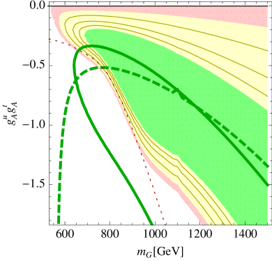
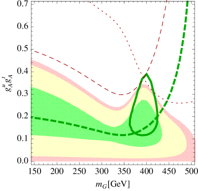
Figure 1: tt¯𝑡¯𝑡t\bar{t} production constraints on the axigluon model in approach B, showing “low” (left plot) and “high” (right plot) mass regions: binned FBA at 1σ1𝜎1\sigma in thick full green line, inclusive CA at 1σ1𝜎1\sigma (2σ2𝜎2\sigma) in thick dashed green line (thin dashed red line), CDF mtt¯subscript𝑚𝑡¯𝑡m_{t\bar{t}} spectrum at 2σ2𝜎2\sigma in thin red dotted line. Parameter regions where the model can improve the SM χ2superscript𝜒2\chi^{2} by Δχ2>0,1,4Δsuperscript𝜒2014-\Delta\chi^{2}>0,1,4 are shaded in red, yellow and green respectively.

IV.1 Axigluon

Among the possible interactions of a heavy color-octet (axial)vector Gsuperscript𝐺G^{\prime}, only the purely axial couplings to uu¯𝑢¯𝑢u\bar{u} (gAusuperscriptsubscript𝑔𝐴𝑢g_{A}^{u}) and tt¯𝑡¯𝑡t\bar{t} (gAtsuperscriptsubscript𝑔𝐴𝑡g_{A}^{t}) currents contribute to the FBA at the tree-level.333Maintaining purely axial quark-axigluon couplings in an electroweak gauge invariant way requires identical couplings to down quarks. However, since at the Tevatron and the LHC, the corresponding dd¯𝑑¯𝑑d\bar{d} parton lumionsities are much smaller than uu¯𝑢¯𝑢u\bar{u}, we neglect the small dd¯𝑑¯𝑑d\bar{d} initial state axigluon contributions to our observables. We thus consider their product gAugAtsuperscriptsubscript𝑔𝐴𝑢superscriptsubscript𝑔𝐴𝑡g_{A}^{u}g_{A}^{t} together with the axigluon mass (mGsubscript𝑚𝐺m_{G}) as the free parameters of the model. Since the effects of a slimit-from𝑠s-channel resonance on the mtt¯subscript𝑚𝑡¯𝑡m_{t\bar{t}} spectrum depend crucially on its width we follow the approach of Barcelo ; Schmalz and assign an axigluon width of ΓG/mG0.2similar-tosubscriptΓ𝐺subscript𝑚𝐺0.2\Gamma_{G}/m_{G}\sim 0.2, deferring the explanation of such a large width to a UV completion of the model. The singular features of an slimit-from𝑠s-channel resonance on tt¯𝑡¯𝑡t\bar{t} spectrum also make the approach B (using the mtt¯subscript𝑚𝑡¯𝑡m_{t\bar{t}} spectrum instead of the total cross-section and inclusive FBA) much preferred for the axigluon model. The results of the global χ2superscript𝜒2\chi^{2} fit together with the impact of individual constraints is presented in Fig. 1. We single out two interesting parameter plane regions as the “low” and “high” mass region focused on the left and the right plots respectively (consistent with results of previous studies, c.f. Bai:2011ed ). We observe that even with the large unexplained axigluon width, axigluon masses which fall within the measured CDF mtt¯subscript𝑚𝑡¯𝑡m_{t\bar{t}} spectrum bins are significantly constrained and in particular cannot improve upon the SM agreement with current experimental results. On the other hand the finite axigluon width effects become insignificant in the “low” region around and below tt¯𝑡¯𝑡t\bar{t} production threshold (for mG450less-than-or-similar-tosubscript𝑚𝐺450m_{G}\lesssim 450 GeV, consistent with the findings of Schmalz ) and in the “high” region above the kinematic reach of the Tevatron (for mG>700subscript𝑚𝐺700m_{G}>700 GeV, as pointed out in Barcelo ). At least in the later, σLHChsubscriptsuperscript𝜎LHC\sigma^{h}_{\rm LHC} mttLHC already contributes a relevant constraint for mG1greater-than-or-equivalent-tosubscript𝑚𝐺1m_{G}\gtrsim 1 TeV and future precise LHC tt¯𝑡¯𝑡t\bar{t} spectrum measurements could have a significant impact. We also note that for this model the tension between FBA and CA measurements is apparent but can be reduced to the 1σ1𝜎1\sigma level. The tension is expected to be larger when symmetric couplings to d𝑑d quarks (as formally required by SM gauge invariance for a pure axigluon) are included AFBvsAC .

IV.2 Zsuperscript𝑍Z^{\prime} and Wsuperscript𝑊W^{\prime}

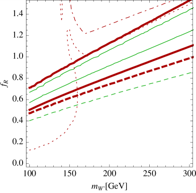
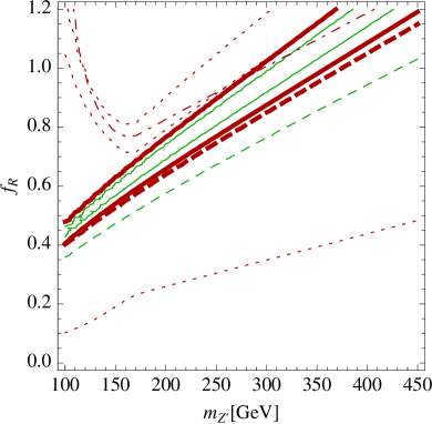
For the Zsuperscript𝑍Z^{\prime} and Wsuperscript𝑊W^{\prime} models we consider only right-handed flavor changing ut𝑢𝑡u-t and dt𝑑𝑡d-t couplings (denoted by fRsubscript𝑓𝑅f_{R}) respectively since these are sufficient to induce a positive FBA contribution. The resulting parameter fits for approach A are represented in Fig. 2.
Refer to caption
Refer to caption
Figure 2: tt¯𝑡¯𝑡t\bar{t} production constraints on the Zsuperscript𝑍Z^{\prime} (left plot) and Wsuperscript𝑊W^{\prime} (right plot) models in approach A: FBA at 1σ1𝜎1\sigma (2σ2𝜎2\sigma)in thin full green line (thick full red line), CA at 1σ1𝜎1\sigma (2σ2𝜎2\sigma) in thin dashed green line (thick dashed red line), σTEVsubscript𝜎TEV\sigma_{\rm TEV} at 2σ2𝜎2\sigma in thin red dotted line, σTEVhsubscriptsuperscript𝜎TEV\sigma^{h}_{\rm TEV} at 2σ2𝜎2\sigma in thin red dash-dotted line. In no parameter region can either of the two models improve upon the SM fit due to the tension between the FBA and CA measurements.

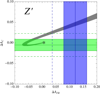
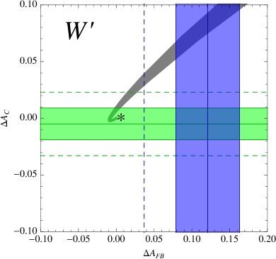
We observe immediately that while a consistent description of tt¯𝑡¯𝑡t\bar{t} observables at the Tevatron can be obtained (in accordance with previous findings Bhattacherjee:2011nr ), these models cannot improve upon the SM results once the LHC measurements are taken into account. This can be traced to the inherent tension between the FBA and CA measurements (and thus independent of approach A or B to the cross-section measurements). For Zsuperscript𝑍Z^{\prime}(Wsuperscript𝑊W^{\prime}) these are tightly correlated (as previously pointed out in AguilarSaavedra:2011vw ), as also illustrated in Fig. 3 where we have varied fRsubscript𝑓𝑅f_{R} within the perturbative regime (|fR|[0,4π]subscript𝑓𝑅04𝜋|f_{R}|\in[0,4\pi]) and the Zsuperscript𝑍Z^{\prime} (Wsuperscript𝑊W^{\prime}) masses in the region mZ(W)[100,500]subscript𝑚superscript𝑍superscript𝑊100500m_{Z^{\prime}(W^{\prime})}\in[100,500] GeV.

Refer to caption
Refer to caption
Figure 3: Correlation between the FBA (ΔAFBΔsubscript𝐴𝐹𝐵\Delta A_{FB}) and CA (ΔACΔsubscript𝐴𝐶\Delta A_{C}) contributions of Zsuperscript𝑍Z^{\prime} (left plot) and Wsuperscript𝑊W^{\prime} (right plot) models in shaded narrow gray bands. The thickness of the bands is given by the Zsuperscript𝑍Z^{\prime} (Wsuperscript𝑊W^{\prime}) mass variation in the range [100,500]100500[100,500] GeV. The Tevatron average of FBA measurements minus the SM prediction at 1σ1𝜎1\sigma (2σ2𝜎2\sigma) is represented by the vertical blue band (dashed vertical lines). The ATLAS measurement of CA minus the SM prediction (the SM reference point is marked with ”*”) at 1σ1𝜎1\sigma (2σ2𝜎2\sigma) is represented by the horizontal green band (dashed horizontal lines). The tension between the two observables increases with increasing mediator mass (inner edge of the band corresponds to lowest mediator mass).

In particular from these plots it is clear that the tension cannot be reduced below the 2σ2𝜎2\sigma level. We also note that the tension increases slightly towards higher Zsuperscript𝑍Z^{\prime} (Wsuperscript𝑊W^{\prime}) masses (when marginalized over the couplings). Consequently, we conclude that these models are excluded as viable FBA explanations and do not consider them any further.

IV.3 Scalar isodoublet

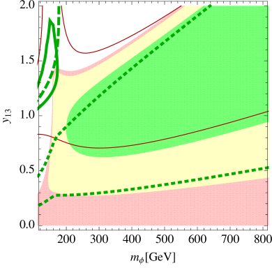
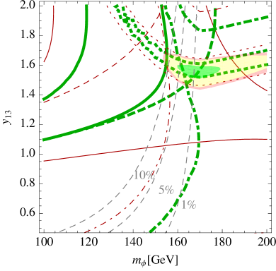
In this model the parameter scan is performed over the u¯RtLsubscript¯𝑢𝑅subscript𝑡𝐿\bar{u}_{R}t_{L} coupling (y13subscript𝑦13y_{13}) and mass (mϕsubscript𝑚italic-ϕm_{\phi}) of the neutral isodoublet component ϕ0superscriptitalic-ϕ0\phi^{0}.444We do not consider the potential dd¯tt¯𝑑¯𝑑𝑡¯𝑡d\bar{d}\to t\bar{t} contributions mediated by the charged isodoublet component, which are suppressed by smaller parton luminosities. The resulting parameter fits for approach A and B are presented in Fig. 4.
Refer to caption
Refer to caption
Figure 4: tt¯𝑡¯𝑡t\bar{t} production constraints on the scalar isodoublet model in approach A (left plot) and B (right plot): FBA (inclusive in left plot and binned in right plot) at 1σ1𝜎1\sigma (2σ2𝜎2\sigma) in thick full green line (thin full red line), inclusive CA at 1σ1𝜎1\sigma (2σ2𝜎2\sigma) in thick dashed green line (thin dashed red line). In left plot σTEVsubscript𝜎TEV\sigma_{\rm TEV} at 1σ1𝜎1\sigma (2σ2𝜎2\sigma) in thick green dotted line (thin red dotted line), σLHCsubscript𝜎LHC\sigma_{\rm LHC} at 1σ1𝜎1\sigma (2σ2𝜎2\sigma) in thick green dash-dotted line (thin red dash-dotted line). In right plot CDF mtt¯subscript𝑚𝑡¯𝑡m_{t\bar{t}} spectrum at 1σ1𝜎1\sigma (2σ2𝜎2\sigma) in thick green dotted line (thin red dotted line). Parameter regions where the model can improve the SM χ2superscript𝜒2\chi^{2} by Δχ2>0,1,4Δsuperscript𝜒2014-\Delta\chi^{2}>0,1,4 are shaded in red, yellow and green respectively. Finally in left plot for mϕ<mtsubscript𝑚italic-ϕsubscript𝑚𝑡m_{\phi}<m_{t}, the contours of constant branching fraction Br(tuϕ0)Br𝑡𝑢superscriptitalic-ϕ0{\rm Br}(t\to u\phi^{0}) are displayed in thin gray dashed lines.

We observe that in approach A (using σTEVsubscript𝜎TEV\sigma_{\rm TEV} and σTEVhsubscriptsuperscript𝜎TEV\sigma^{h}_{\rm TEV}) there is a small preferred parameter region at low ϕ0superscriptitalic-ϕ0\phi^{0} masses (mϕmtless-than-or-similar-tosubscript𝑚italic-ϕsubscript𝑚𝑡m_{\phi}\lesssim m_{t}, consistent with findings of doublet ). Interestingly, mϕsubscript𝑚italic-ϕm_{\phi} is bounded from below by the LHC inclusive cross-section measurement. This is because the new tϕ0u𝑡superscriptitalic-ϕ0𝑢t\to\phi^{0}u decay channel tends to suppress the reconstructed cross-sections (see Eq. (15)) irrespective of the production mechanism inducing a tension between the Tevatron and LHC results. When considering instead the complete CDF mtt¯subscript𝑚𝑡¯𝑡m_{t\bar{t}} spectrum (approach B), the mϕmtless-than-or-similar-tosubscript𝑚italic-ϕsubscript𝑚𝑡m_{\phi}\lesssim m_{t} region is no longer favored. This happens because a light scalar exchanged in the tlimit-from𝑡t-channel tends to harden the dσ/dmtt¯𝑑𝜎𝑑subscript𝑚𝑡¯𝑡d\sigma/dm_{t\bar{t}} spectrum compared to SM QCD predictions, inducing a tension with the binned spectrum measurement by CDF (in this particular case, the discrepancy is most pronounced in the lowest mtt¯subscript𝑚𝑡¯𝑡m_{t\bar{t}} bin which was measured precisely by CDF CDFmtt ). Given our rough treatment of the correlated uncertainties entering dσTEV/dmtt¯𝑑subscript𝜎TEV𝑑subscript𝑚𝑡¯𝑡d\sigma_{\rm TEV}/dm_{t\bar{t}} and also the neglect of subleading SM contributions Manohar:2012rs , we shall keep the low mass region, disfavored by the dσ/dmtt¯𝑑𝜎𝑑subscript𝑚𝑡¯𝑡d\sigma/dm_{t\bar{t}} observables, in our analysis. What remains in addition is a less interesting intermediate to heavy ϕ0superscriptitalic-ϕ0\phi^{0} mass region (mϕ>200subscript𝑚italic-ϕ200m_{\phi}>200 GeV) where the FBA cannot be reproduced at the 1σ1𝜎1\sigma level however the overall agreement with the present experimental data is improved with respect to the SM (in order to clearly distinguish it from the light ϕ0superscriptitalic-ϕ0\phi^{0} region, we shall only consider parameter values where the overall fit improvement with respect to the SM is at least Δχ2>4Δsuperscript𝜒24-\Delta\chi^{2}>4, shaded green in right plot of Fig. 4). Finally in this model the tension between the inclusive FBA and CA measurements can be reduced below the 2σ2𝜎2\sigma level, even though the 68%percent6868\% CL regions for both observables cannot be reached simultaneously.

IV.4 Scalar color triplet and sextet

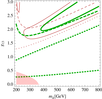
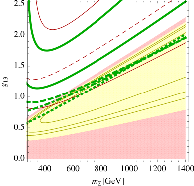
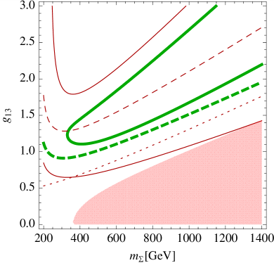
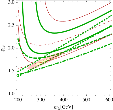
We consider chiral couplings of ΔΔ\Delta and ΣΣ\Sigma to right-handed di-quark currents u¯RtRCsubscript¯𝑢𝑅superscriptsubscript𝑡𝑅𝐶\bar{u}_{R}t_{R}^{C} with a coupling constant g13subscript𝑔13g_{13}. The results of the corresponding parameter fits are presented in Figs. 5 and 6.
Refer to caption
Refer to caption
Figure 5: tt¯𝑡¯𝑡t\bar{t} production constraints on the scalar color triplet model in approach A (left plot) and B (right plot): FBA (inclusive in left plot and binned in right plot) at 1σ1𝜎1\sigma (2σ2𝜎2\sigma) in thick full green line (thin full red line), inclusive CA at 1σ1𝜎1\sigma (2σ2𝜎2\sigma) in thick dashed green line (thin dashed red line). In left plot σTEVsubscript𝜎TEV\sigma_{\rm TEV} at 1σ1𝜎1\sigma (2σ2𝜎2\sigma) in thick green dotted line (thin red dotted line), σTEVhsubscriptsuperscript𝜎TEV\sigma^{h}_{\rm TEV} at 2σ2𝜎2\sigma in thin red dash-dotted line. In right plot CDF mtt¯subscript𝑚𝑡¯𝑡m_{t\bar{t}} spectrum at 1σ1𝜎1\sigma (2σ2𝜎2\sigma) in thick green dotted line (thin red dotted line). Parameter regions where the model can improve the SM χ2superscript𝜒2\chi^{2} by Δχ2>0,1Δsuperscript𝜒201-\Delta\chi^{2}>0,1 are shaded in red and yellow respectively.
Refer to caption
Refer to caption
Figure 6: tt¯𝑡¯𝑡t\bar{t} production constraints on the scalar color sextet model in approach A (left plot) and B (right plot): FBA (inclusive in left plot and binned in right plot) at 1σ1𝜎1\sigma (2σ2𝜎2\sigma) in thick full green line (thin full red line), inclusive CA at 2σ2𝜎2\sigma in thin dashed red line. In left plot σTEVsubscript𝜎TEV\sigma_{\rm TEV} at 1σ1𝜎1\sigma in thick green dotted line, σTEVhsubscriptsuperscript𝜎TEV\sigma^{h}_{\rm TEV} at 1σ1𝜎1\sigma in thick green dash-dotted line. In right plot CDF mtt¯subscript𝑚𝑡¯𝑡m_{t\bar{t}} spectrum at 2σ2𝜎2\sigma in thin red dotted line. Parameter regions where the model can improve the SM χ2superscript𝜒2\chi^{2} by χ2>0,1superscript𝜒201-\chi^{2}>0,1 are shaded in red and yellow respectively.

Both of these models experience a tension between the FBA and the tt¯𝑡¯𝑡t\bar{t} spectrum measurements Gresham , in particular at high mtt¯subscript𝑚𝑡¯𝑡m_{t\bar{t}}. While in approach A an overall improvement in the goodness of fit can still be obtained in some parameter regions of the two models (see left plots in Figs. 5 and 6); taking into account the complete binned mtt¯subscript𝑚𝑡¯𝑡m_{t\bar{t}} spectrum measurement by CDF removes these preferred regions and the FBA discrepancy can no longer be addressed. Again, taking into account the possible caveats of the dσ/dmtt¯𝑑𝜎𝑑subscript𝑚𝑡¯𝑡d\sigma/dm_{t\bar{t}} constraints, we shall keep the ΔΔ\Delta and ΣΣ\Sigma model parameter regions preferred in approach A in our analysis of top spin observables.

V TOP SPIN OBSERVABLES

V.1 Definitions

Since the spin information of a decaying top quark is not diluted by hadronization it is possible to investigate various top-spin polarization effects at hadron colliders. The starting point is the calculation of the production spin density matrices for the dominant partonic production channels of top quark pairs,

q(p1)+q¯(p2)t(k1,st)+t¯(k2,st¯),superscriptabsent𝑞subscript𝑝1¯𝑞subscript𝑝2𝑡subscript𝑘1subscript𝑠𝑡¯𝑡subscript𝑘2subscript𝑠¯𝑡\displaystyle q(p_{1})+\overline{q}(p_{2})\stackrel{{\scriptstyle}}{{\to}}t(k_{1},s_{t})+\overline{t}(k_{2},s_{\overline{t}})\,,
g(p1)+g(p2)t(k1,st)+t¯(k2,st¯),superscriptabsent𝑔subscript𝑝1𝑔subscript𝑝2𝑡subscript𝑘1subscript𝑠𝑡¯𝑡subscript𝑘2subscript𝑠¯𝑡\displaystyle g(p_{1})+g(p_{2})\stackrel{{\scriptstyle}}{{\to}}t(k_{1},s_{t})+\overline{t}(k_{2},s_{\overline{t}})\,, (16)

via the relevant scattering amplitudes Isubscript𝐼\mathcal{M}_{I} where I=qq¯,gg𝐼𝑞¯𝑞𝑔𝑔I=q\overline{q},gg. The differential cross sections for these partonic processes can be written as dσI(st,st¯)=ΦI|I|2dΓtt¯𝑑subscript𝜎𝐼subscript𝑠𝑡subscript𝑠¯𝑡subscriptΦ𝐼superscriptsubscript𝐼2𝑑subscriptΓ𝑡¯𝑡d\sigma_{I}(s_{t},s_{\overline{t}})=\Phi_{I}|\mathcal{M}_{I}|^{2}d\Gamma_{t\bar{t}} where ΦIsubscriptΦ𝐼\Phi_{I} is the relevant initial state flux normalization and dΓtt¯𝑑subscriptΓ𝑡¯𝑡d\Gamma_{t\bar{t}} is the tt¯𝑡¯𝑡t\bar{t} phase space differential. The problem is thus reduced to evaluating the absolute squares of the relevant polarized scattering amplitudes

|I|2=14Tr[ρI(𝟏+𝐬^t𝝈)(𝟏+𝐬^t¯𝝈)],superscriptsubscript𝐼214Trdelimited-[]tensor-productsubscript𝜌𝐼1subscript^𝐬𝑡𝝈1subscript^𝐬¯𝑡𝝈\displaystyle|\mathcal{M}_{I}|^{2}=\frac{1}{4}{\rm Tr}[\rho_{I}({\bf 1}+\mathbf{\hat{s}}_{t}\cdot\boldsymbol{\sigma})\otimes({\bf 1}+\mathbf{\hat{s}}_{\overline{t}}\cdot\boldsymbol{\sigma})]\,, (17)

where ρIsubscript𝜌𝐼\rho_{I} is the corresponding partonic production spin density matrix describing the production of (on-shell) top quark pairs in a specific spin configuration, while 𝐬^tsubscript^𝐬𝑡\mathbf{\hat{s}}_{t} (𝐬^t¯subscript^𝐬¯𝑡\mathbf{\hat{s}}_{\overline{t}}) is the unit polarization vector of the top (anti top) quark in its rest frame and 𝝈=(σ1,σ2,σ3)T𝝈superscriptsubscript𝜎1subscript𝜎2subscript𝜎3𝑇\boldsymbol{\sigma}=(\sigma_{1},\sigma_{2},\sigma_{3})^{T} is a vector of Pauli matrices.

Conveniently, one starts with the most general decomposition of the spin density matrix ρ𝜌\rho (suppressing the initial state subscript I𝐼I) for the production of a top quark pair

ρ=A 1𝟏+Bitσi𝟏+Bit¯ 1σi+Cijσiσj,𝜌tensor-product𝐴11tensor-productsuperscriptsubscript𝐵𝑖𝑡subscript𝜎𝑖1tensor-productsuperscriptsubscript𝐵𝑖¯𝑡1subscript𝜎𝑖tensor-productsubscript𝐶𝑖𝑗subscript𝜎𝑖subscript𝜎𝑗\displaystyle\rho=A\,{\bf 1}\otimes{\bf 1}+B_{i}^{t}\,\sigma_{i}\otimes{\bf 1}+B_{i}^{\overline{t}}\,{\bf 1}\otimes\sigma_{i}+C_{ij}\,\sigma_{i}\otimes\sigma_{j}\,, (18)

where the functions A𝐴A, Bitsuperscriptsubscript𝐵𝑖𝑡{B}_{i}^{t} (Bit¯superscriptsubscript𝐵𝑖¯𝑡{B}_{i}^{\overline{t}}) and Cijsubscript𝐶𝑖𝑗C_{ij} describe the spin-averaged production cross section, polarization of a top (anti top) quarks and the top - anti top spin-spin correlations, respectively. Using the spin four-vectors defined as

stμsuperscriptsubscript𝑠𝑡𝜇\displaystyle s_{t}^{\mu} =\displaystyle= (𝐤1𝐬^tmt,𝐬^t+𝐤1(𝐤1𝐬^t)mt(Et+mt)),subscript𝐤1subscript^𝐬𝑡subscript𝑚𝑡subscript^𝐬𝑡subscript𝐤1subscript𝐤1subscript^𝐬𝑡subscript𝑚𝑡subscript𝐸𝑡subscript𝑚𝑡\displaystyle\left(\frac{\mathbf{k}_{1}\cdot\mathbf{\hat{s}}_{t}}{m_{t}},\mathbf{\hat{s}}_{t}+\frac{\mathbf{k}_{1}(\mathbf{k}_{1}\cdot\hat{\mathbf{s}}_{t})}{m_{t}(E_{t}+m_{t})}\right)\,,
st¯μsuperscriptsubscript𝑠¯𝑡𝜇\displaystyle s_{\overline{t}}^{\mu} =\displaystyle= (𝐤2𝐬^t¯mt,𝐬^t¯+𝐤2(𝐤2𝐬^t¯)mt(Et¯+mt)),subscript𝐤2subscript^𝐬¯𝑡subscript𝑚𝑡subscript^𝐬¯𝑡subscript𝐤2subscript𝐤2subscript^𝐬¯𝑡subscript𝑚𝑡subscript𝐸¯𝑡subscript𝑚𝑡\displaystyle\left(\frac{\mathbf{k}_{2}\cdot\mathbf{\hat{s}}_{\overline{t}}}{m_{t}},\mathbf{\hat{s}}_{\overline{t}}+\frac{\mathbf{k}_{2}(\mathbf{k}_{2}\cdot\mathbf{\hat{s}}_{\overline{t}})}{m_{t}(E_{\bar{t}}+m_{t})}\right)\,, (19)

the decomposition of the squared scattering amplitude ||2superscript2|\mathcal{M}|^{2} can be written as

||2=a+bμtstμ+bμt¯st¯μ+cμνstμst¯ν,superscript2𝑎subscriptsuperscript𝑏𝑡𝜇superscriptsubscript𝑠𝑡𝜇subscriptsuperscript𝑏¯𝑡𝜇superscriptsubscript𝑠¯𝑡𝜇subscript𝑐𝜇𝜈superscriptsubscript𝑠𝑡𝜇superscriptsubscript𝑠¯𝑡𝜈\displaystyle|\mathcal{M}|^{2}=a+b^{t}_{\mu}s_{t}^{\mu}+b^{\overline{t}}_{\mu}s_{\overline{t}}^{\mu}+c_{\mu\nu}s_{t}^{\mu}s_{\overline{t}}^{\nu}\,, (20)

and by comparing expressions (18) and (20) one can extract the functions A𝐴A, Bitsuperscriptsubscript𝐵𝑖𝑡{B}_{i}^{t} (Bit¯superscriptsubscript𝐵𝑖¯𝑡{B}_{i}^{\overline{t}}) and Cijsubscript𝐶𝑖𝑗C_{ij}. With this at hand, the various top spin observables 𝒪delimited-⟨⟩𝒪\langle{\cal O}\rangle can be calculated as

𝒪(𝐒t,𝐒t¯)I=ΦIσI𝑑Γtt¯Tr[ρI𝒪(𝐒t,𝐒t¯)],subscriptdelimited-⟨⟩𝒪subscript𝐒𝑡subscript𝐒¯𝑡𝐼subscriptΦ𝐼subscript𝜎𝐼differential-dsubscriptΓ𝑡¯𝑡Trdelimited-[]subscript𝜌𝐼𝒪subscript𝐒𝑡subscript𝐒¯𝑡\displaystyle\langle{\cal O}(\mathbf{{S}}_{t},\mathbf{{S}}_{\overline{t}})\rangle_{I}=\frac{\Phi_{I}}{\sigma_{I}}\int d\Gamma_{t\bar{t}}{{\rm Tr}[\rho_{I}\cdot{\cal O}(\mathbf{{S}}_{t},\mathbf{{S}}_{\overline{t}})]}\,, (21)

where σI=ΦI𝑑Γtt¯Tr[ρI]subscript𝜎𝐼subscriptΦ𝐼differential-dsubscriptΓ𝑡¯𝑡Trdelimited-[]subscript𝜌𝐼\sigma_{I}=\Phi_{I}\int d\Gamma_{t\bar{t}}{\rm Tr}[\rho_{I}] is the unpolarized production cross-section and 𝐒t=𝝈/2𝟏(𝐒t¯=𝟏𝝈/2)subscript𝐒𝑡tensor-product𝝈21subscript𝐒¯𝑡tensor-product1𝝈2\mathbf{{S}}_{t}=\boldsymbol{\sigma}/2\otimes{\bf 1}\,(\mathbf{{S}}_{\overline{t}}={\bf 1}\otimes\boldsymbol{\sigma}/2) is the top (anti top) spin operator. In particular, we consider the following spin observables

𝒪1subscript𝒪1\displaystyle{\cal O}_{1} =\displaystyle= 𝐒t𝐒t¯,subscript𝐒𝑡subscript𝐒¯𝑡\displaystyle\mathbf{{S}}_{t}\cdot\mathbf{S}_{\overline{t}}\,,
𝒪2subscript𝒪2\displaystyle{\cal O}_{2} =\displaystyle= 𝐒t𝐚^,𝒪¯2=𝐒t¯𝐛^,subscript𝐒𝑡^𝐚subscript¯𝒪2subscript𝐒¯𝑡^𝐛\displaystyle\mathbf{{S}}_{t}\cdot\mathbf{\hat{a}}\,,\quad\bar{\cal O}_{2}=\mathbf{{S}}_{\bar{t}}\cdot\mathbf{\hat{b}}\,,
𝒪3subscript𝒪3\displaystyle{\cal O}_{3} =\displaystyle= 4(𝐒t𝐚^)(𝐒t¯𝐛^),4subscript𝐒𝑡^𝐚subscript𝐒¯𝑡^𝐛\displaystyle 4(\mathbf{{S}}_{t}\cdot\mathbf{\hat{a}})(\mathbf{S}_{\overline{t}}\cdot\mathbf{\hat{b}})\,, (22)

which give the net spin polarization of the top - anti top system, polarization of the (anti) top quark, and the top - anti top spin correlation both with respect to spin quantization axes 𝐚^^𝐚\mathbf{\hat{a}} and 𝐛^^𝐛\mathbf{\hat{b}}, respectively. At the parton level 𝒪3subscript𝒪3{\cal O}_{3} is related to the spin correlation function Cijsubscript𝐶𝑖𝑗C_{ij} in Eq. (18), namely

𝒪3=σtt¯()+σtt¯()σtt¯()σtt¯()σtt¯()+σtt¯()+σtt¯()+σtt¯(),\displaystyle\braket{{\cal O}_{3}}=\frac{\sigma_{t\bar{t}}(\uparrow\uparrow)+\sigma_{t\bar{t}}(\downarrow\downarrow)-\sigma_{t\bar{t}}(\uparrow\downarrow)-\sigma_{t\bar{t}}(\downarrow\uparrow)}{\sigma_{t\bar{t}}(\uparrow\uparrow)+\sigma_{t\bar{t}}(\downarrow\downarrow)+\sigma_{t\bar{t}}(\uparrow\downarrow)+\sigma_{t\bar{t}}(\downarrow\uparrow)}\,, (23)

where the arrows refer to the up and down spin orientations of the top and the anti top quark with respect to the 𝐚^^𝐚\mathbf{\hat{a}} and 𝐛^^𝐛\mathbf{\hat{b}} quantization axes, respectively. It can be measured using the double differential angular distribution of the top and anti top quark decay products:

1σd2σdcosθfdcosθf¯=14(1+Btcosθf+Bt¯cosθf¯Ccosθfcosθf¯),1𝜎superscript𝑑2𝜎𝑑subscript𝜃𝑓𝑑subscript𝜃¯𝑓141subscript𝐵𝑡subscript𝜃𝑓subscript𝐵¯𝑡subscript𝜃¯𝑓𝐶subscript𝜃𝑓subscript𝜃¯𝑓\displaystyle\frac{1}{\sigma}\frac{d^{2}\sigma}{d\cos\theta_{f}d\cos\theta_{\bar{f}}}=\frac{1}{4}\left(1+B_{t}\cos\theta_{f}+B_{\bar{t}}\cos\theta_{\bar{f}}-C\cos\theta_{f}\cos\theta_{\bar{f}}\right)\,, (24)

where θf(θf¯)subscript𝜃𝑓subscript𝜃¯𝑓\theta_{f}(\theta_{\bar{f}}) is the angle between the direction of the top (anti top) spin analyzer f,(f¯)𝑓¯𝑓f,\,(\bar{f}) (which can be either a direct t𝑡t (t¯¯𝑡\bar{t}) daughter W+,bsuperscript𝑊𝑏W^{+},b (W,b¯superscript𝑊¯𝑏W^{-},\bar{b}) or a W+(W)superscript𝑊superscript𝑊W^{+}(W^{-}) decay product +(),ν(ν¯)superscriptsuperscript𝜈¯𝜈\ell^{+}(\ell^{-}),\nu(\bar{\nu}) or jets) in the t𝑡t (t¯)¯𝑡(\bar{t}) rest frame and the 𝐚^^𝐚\hat{\bf a} (𝐛^^𝐛\hat{\bf b}) direction in the tt¯𝑡¯𝑡t\bar{t} center of mass frame (when the corresponding frame transformation is a rotation free boost, c.f. spinSM ). Analogously 𝒪2subscript𝒪2{\cal O}_{2} and 𝒪¯2subscript¯𝒪2\bar{\cal O}_{2} are related to the (anti)top spin polarization coefficients Btsubscript𝐵𝑡B_{t} and Bt¯subscript𝐵¯𝑡B_{\bar{t}}. We note in passing that in absence of CP violation BBt=Bt¯𝐵subscript𝐵𝑡minus-or-plussubscript𝐵¯𝑡B\equiv B_{t}=\mp B_{\bar{t}} for 𝐚^=±𝐛^^𝐚plus-or-minus^𝐛\hat{\bf a}=\pm\hat{\bf b}. For perfect (anti)top spin analyzers whose flight directions are 100%percent100100\% correlated with the directions of the (anti)top spin then

𝒪3=C,𝒪2=Bt,𝒪¯2=Bt¯.formulae-sequenceexpectationsubscript𝒪3𝐶formulae-sequenceexpectationsubscript𝒪2subscript𝐵𝑡expectationsubscript¯𝒪2subscript𝐵¯𝑡\braket{\mathcal{O}_{3}}=C\,,\quad\braket{\mathcal{O}_{2}}=B_{t}\,,\quad\braket{\bar{\mathcal{O}}_{2}}=B_{\bar{t}}\,. (25)

This limit is a good approximation for the charged leptons from W𝑊W decays Brandenburg:2002xr . For other (anti)top spin analyzers one needs to apply the corresponding top spin analyzing power factors κf(f¯)subscript𝜅𝑓¯𝑓\kappa_{f(\bar{f})} (where κ+()1similar-to-or-equalssubscript𝜅superscriptsuperscript1\kappa_{\ell^{+}(\ell^{-})}\simeq 1) in Eq. (24) as

CCκfκf¯,Bt(t¯)Bt(t¯)κf(f¯).formulae-sequence𝐶𝐶subscript𝜅𝑓subscript𝜅¯𝑓subscript𝐵𝑡¯𝑡subscript𝐵𝑡¯𝑡subscript𝜅𝑓¯𝑓C\to C\kappa_{f}\kappa_{\bar{f}}\,,\quad B_{t(\bar{t})}\to B_{t(\bar{t})}\kappa_{f(\bar{f})}\,. (26)

The values of κf(f¯)subscript𝜅𝑓¯𝑓\kappa_{f(\bar{f})} are presently known at NLO in QCD and can be found in Brandenburg:2002xr . Finally, 𝒪1subscript𝒪1{\cal O}_{1} can be probed using the spin analyzer opening angle distribution

1σdσdcosϕ=12(1Dcosϕ),1𝜎𝑑𝜎𝑑italic-ϕ121𝐷italic-ϕ\displaystyle\frac{1}{\sigma}\frac{d\sigma}{d\cos\phi}=\frac{1}{2}\left(1-D\cos\phi\right)\,, (27)

where ϕitalic-ϕ\phi is the angle between the direction of flight of the two (top and anti top) spin analyzers, defined in the t𝑡t and t¯¯𝑡\bar{t} frames, respectively. Again, for f=+𝑓superscriptf=\ell^{+}, f¯=¯𝑓superscript\bar{f}=\ell^{-} one then obtains

𝒪1=D,expectationsubscript𝒪1𝐷\braket{\mathcal{O}_{1}}=D\,, (28)

while for other spin analyzers the appropriate κf(f¯)subscript𝜅𝑓¯𝑓\kappa_{f(\bar{f})} corrections should be applied.

The arbitrary unit vectors 𝐚^^𝐚\bf{\hat{a}} and 𝐛^^𝐛\bf{\hat{b}} specify different spin quantization axes which can be chosen to maximize the desired polarization and correlation effects. We work with the following choices:

𝐚^^𝐚\displaystyle\hat{\bf a} =𝐛^=𝐤^1,absent^𝐛subscript^𝐤1\displaystyle=-\hat{\bf b}=\hat{\bf k}_{1}\,, (``helicity"basis),``helicity"basis\displaystyle({\rm``helicity"\;basis})\,,
𝐚^^𝐚\displaystyle\hat{\bf a} =𝐛^=𝐩^,absent^𝐛^𝐩\displaystyle=\hat{\bf b}=\hat{\bf p}\,, (``beamline"basis),``beamline"basis\displaystyle({\rm``beamline"\;basis})\,,
𝐚^^𝐚\displaystyle\hat{\bf a} =𝐛^=𝐝^X,absent^𝐛subscript^𝐝𝑋\displaystyle=\hat{\bf b}=\hat{\bf d}_{X}\,, (``offdiagonal"basis,specificformodelX),``offdiagonal"basisspecificformodelX\displaystyle({\rm``off-diagonal"\;basis,\;specific\;for\;model\;X})\,, (29)

where 𝐩^^𝐩\hat{\bf p} is the direction of the incoming beam and 𝐤^1subscript^𝐤1\hat{\bf k}_{1} is the direction of the outgoing top quark, both in the tt¯𝑡¯𝑡t\bar{t} center of mass frame.

By the detailed study of the top (anti top) decay products one can obtain valuable information about top spin observables and use them to distinguish among the different models addressing the FBA puzzle. In order to maximize top spin effects it is advisable to choose a proper spin quantization axis. For the leading order QCD quark-antiquark annihilation dominating the tt¯𝑡¯𝑡t\bar{t} production at the Tevatron, a special off-diagonal axis was shown to exist Parke:1996pr , for which the top spins are 100%percent100100\% correlated. It is given by quantizing the spins with the axis 𝐝^qq¯,SMsubscript^𝐝𝑞¯𝑞SM\hat{\bf d}_{q\bar{q},\rm SM} determined as

𝐝^qq¯,SM=𝐩^+(1γ)z𝐤^11(1γ2)z2,subscript^𝐝𝑞¯𝑞SM^𝐩1𝛾𝑧subscript^𝐤111superscript𝛾2superscript𝑧2\displaystyle\hat{\bf d}_{q\bar{q},\rm SM}=\frac{-\hat{\bf p}+(1-\gamma)z\;\hat{\bf k}_{1}}{\sqrt{1-(1-\gamma^{2})z^{2}}}\,, (30)

where z=𝐩^𝐤^1=cosθ𝑧^𝐩subscript^𝐤1𝜃z=\hat{\bf p}\cdot\hat{\bf k}_{1}=\cos\theta and γ=Et/mt=1/1β2𝛾subscript𝐸𝑡subscript𝑚𝑡11superscript𝛽2\gamma=E_{t}/m_{t}=1/\sqrt{1-\beta^{2}} and interpolates between the beamline basis at the threshold (γ1𝛾1\gamma\to 1) and the helicity basis for ultrarelativistic energies (γ𝛾\gamma\to\infty). There is no such optimal axis for the gluon-gluon fusion process (dominating the tt¯𝑡¯𝑡t\bar{t} production at the LHC)555At low mtt¯subscript𝑚𝑡¯𝑡m_{t\bar{t}} the top quark pair production via gluon-gluon fusion is dominated by like-helicity gluons. Consequently, spin correlations are maximal in the helicity basis Mahlon:2010gw ., but it is always possible to find a basis, in which spin correlations are maximal. A general procedure for finding such an off-diagonal basis is given in Mahlon:1997uc ; Uwer:2004vp . The idea is to determine the maximal eigenvalue of the matrix function Cijsubscript𝐶𝑖𝑗C_{ij} in Eq. (18) and the corresponding eigenvector, which provides the off-diagonal quantization axis 𝐝^Xsubscript^𝐝𝑋\hat{\bf d}_{X}. Such an off-diagonal axis can be constructed for any model. As an example we present the explicit formula for the axigluon model (see also Bai:2011uk )

𝐝^A=𝐩^+((1γ)zgA2γ21ssmA2)𝐤^11(1γ2)z2+2γγ21gA2s/(smA2)z(1γ2)gA4s2/(smA2)2,subscript^𝐝𝐴^𝐩1𝛾𝑧superscriptsubscript𝑔𝐴2superscript𝛾21𝑠𝑠superscriptsubscript𝑚𝐴2subscript^𝐤111superscript𝛾2superscript𝑧22𝛾superscript𝛾21superscriptsubscript𝑔𝐴2𝑠𝑠superscriptsubscript𝑚𝐴2𝑧1superscript𝛾2superscriptsubscript𝑔𝐴4superscript𝑠2superscript𝑠superscriptsubscript𝑚𝐴22\displaystyle\hat{\bf d}_{A}=\frac{-\hat{\bf p}+\left((1-\gamma)z-g_{A}^{2}\sqrt{\gamma^{2}-1}\frac{s}{s-m_{A}^{2}}\right)\,\hat{\bf k}_{1}}{\sqrt{1-(1-\gamma^{2})z^{2}+2\gamma\sqrt{\gamma^{2}-1}g_{A}^{2}s/(s-m_{A}^{2})z-(1-\gamma^{2})g_{A}^{4}s^{2}/(s-m_{A}^{2})^{2}}}\,, (31)

where gAsubscript𝑔𝐴g_{A} and mGsubscript𝑚𝐺m_{G} are free parameters of the axis. The qq¯𝑞¯𝑞q\bar{q} annihilation induced top spin correlations in this basis are maximal when these parameters match the actual axigluon resonance parameters (i.e. when gA=gAugAtsubscript𝑔𝐴superscriptsubscript𝑔𝐴𝑢superscriptsubscript𝑔𝐴𝑡g_{A}=g_{A}^{u}g_{A}^{t} and mA=mGsubscript𝑚𝐴subscript𝑚𝐺m_{A}=m_{G}). It turns out however, that such custom axes are not necessarily better in discriminating between the SM and NP contributions to top pair production via qq¯𝑞¯𝑞q\bar{q} annihilation. This can be easily understood by treating the SM and SM+NP as two competing hypotheses, among which we wish do discriminate using top spin correlations. Then the SM qq¯𝑞¯𝑞q\bar{q} off-diagonal axis is already optimal for one of the hypotheses (it maximizes the leading QCD qq¯𝑞¯𝑞q\bar{q} induced spin correlations) and is furthermore completely fixed by known SM parameters. Conversely any NP model off-diagonal axis needs to reduce to the SM one in the limit where the NP parameters determining the NP off-diagonal basis decouple (gA0subscript𝑔𝐴0g_{A}\to 0 and/or mAsubscript𝑚𝐴m_{A}\to\infty for the axigluon axis in Eq. (31)). In the case of the axigluon model off-diagonal axis, we have checked explicitly, that in the interesting regions of parameter space and for arbitrary values of gA,mAsubscript𝑔𝐴subscript𝑚𝐴g_{A},m_{A}, the axigluon predictions do not deviate from SM values significantly more than in the helicity or the SM qq¯𝑞¯𝑞q\bar{q} off-diagonal axis. Consequently, in our numerical study we use the helicity (for spin correlation Chelsubscript𝐶helC_{\rm hel} and polarization Bhelsubscript𝐵helB_{\rm hel} coefficients), beamline (for Cbeamsubscript𝐶beamC_{\rm beam}, Bbeamsubscript𝐵beamB_{\rm beam}) and SM qq¯𝑞¯𝑞q\bar{q} off-diagonal (for Coffsubscript𝐶offC_{\rm off}, Boffsubscript𝐵offB_{\rm off}) spin quantization axes defined in Eqs. (29) and (30) respectively.

V.2 Results

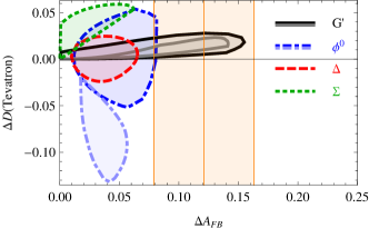
In this section we present predictions for the various top spin observables at the Tevatron as well as the 777 TeV (and 888 TeV) LHC within the various NP model parameter regions which are able to address the FBA puzzle, as determined in Sec. IV. In particular we present correlations between the inclusive and high mtt¯subscript𝑚𝑡¯𝑡m_{t\bar{t}} FBA values as measured at the Tevatron, and the shifts of the various spin observables from their corresponding SM values. We define (see Sec. III) ΔAFBAFBAFBSMΔsubscript𝐴𝐹𝐵subscript𝐴𝐹𝐵superscriptsubscript𝐴𝐹𝐵SM\Delta A_{FB}\equiv A_{FB}-A_{FB}^{\rm SM}, ΔCiCiCiSMΔsubscript𝐶𝑖subscript𝐶𝑖superscriptsubscript𝐶𝑖SM\Delta C_{i}\equiv C_{i}-C_{i}^{\rm SM} and ΔDDDSMΔ𝐷𝐷superscript𝐷SM\Delta D\equiv D-D^{\rm SM}. On the other hand since QCD produced top quarks are not polarized, (neglecting tiny electroweak contributions) we assume BiSM0similar-to-or-equalssuperscriptsubscript𝐵𝑖SM0B_{i}^{\rm SM}\simeq 0 and present results for Bisubscript𝐵𝑖B_{i} in presence of NP directly. The predictions for the relevant spin observables at the Tevatron are shown in Fig. 7.
Refer to caption
Refer to caption
Refer to caption
Refer to caption
Refer to caption
Refer to caption
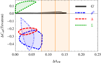
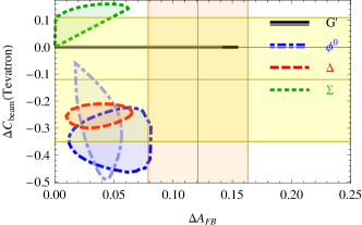
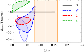
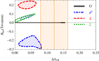
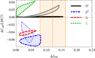
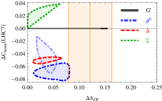
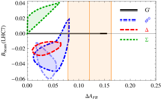
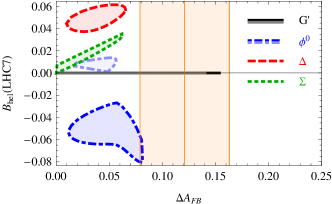
Figure 7: Correlations between the NP contributions to the inclusive FBA and various spin observables at the Tevatron (see text for details and definitions). The present experimental results (68%percent6868\% C.L. regions) are shaded in horizontal and vertical bands. The NP model predictions are determined from the global fit as specified in Sec. IV and are bounded by full (axigluon Gsuperscript𝐺G^{\prime} in the low (mG450less-than-or-similar-tosubscript𝑚𝐺450m_{G}\lesssim 450 GeV in black) and high (mG700greater-than-or-equivalent-tosubscript𝑚𝐺700m_{G}\gtrsim 700 GeV in gray) mass regions), dashed (scalar color triplet ΔΔ\Delta), dotted (scalar color sextet ΣΣ\Sigma) and dot-dashed (neutral component of the scalar isodoublet ϕ0superscriptitalic-ϕ0\phi^{0} in the low (mϕmtless-than-or-similar-tosubscript𝑚italic-ϕsubscript𝑚𝑡m_{\phi}\lesssim m_{t} in darker shade) and high (mϕ>200subscript𝑚italic-ϕ200m_{\phi}>200 GeV in lighter shade) mass region) contours.

First note that the results for the SM qq¯𝑞¯𝑞q\bar{q} off-diagonal axis at the Tevatron turn out to be almost identical to the beamline axis (and very similar at the LHC, see Fig. 8). Both bases provide good potential discrimination between color sextet on one hand, and color triplet or isodoublet scalar models on the other hand. The off-diagonal basis exhibits marginally better sensitivity only for the axigluon (Gsuperscript𝐺G^{\prime}) model. However, since purely axial couplings of Gsuperscript𝐺G^{\prime} to quarks do not produce polarized top quarks, Bisubscript𝐵𝑖B_{i} vanishes for the axigluon model and consequently we do not plot Boffsubscript𝐵offB_{\rm off} dependence separately.

We observe that existing spin observable measurements at the Tevatron do not overly constrain selected NP models. Some sensitivity to the light scalar isodoublet model is exhibited by the recent beamline axis spin correlation measurement by DØ spinTEV1 as seen in the center left plot in Fig. 7. On the other hand (anti)top polarization (Bisubscript𝐵𝑖B_{i} both in the beamline and in the helicity basis) offers a very powerful probe of scalar t𝑡t-channel models and a 𝒪(20%)𝒪percent20\mathcal{O}(20\%) precision measurement (in helicity basis) could already test (and discriminate between) the scalar color triplet (ΔΔ\Delta) and isodoublet (ϕ0superscriptitalic-ϕ0\phi^{0}) model explanations of the FBA. Finally, the axigluon (Gsuperscript𝐺G^{\prime}) models in general give very small contributions to the chosen spin observables. For example, at the Tevatron, spin correlation measurements at 𝒪(2%)𝒪percent2\mathcal{O}(2\%) precision would be required to probe such FBA explanations.

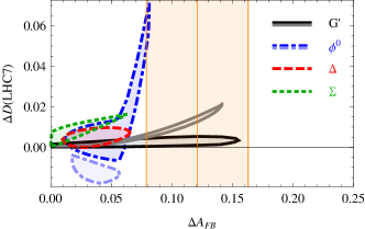
The results for the relevant spin observables at the 7 TeV LHC are shown in Fig. 8.666The results for ΔDΔ𝐷\Delta D, ΔCiΔsubscript𝐶𝑖\Delta C_{i} and Bisubscript𝐵𝑖B_{i} at the 7 TeV and 8 TeV LHC are almost identical and we do not show the later separately.
Refer to caption
Refer to caption
Refer to caption
Refer to caption
Refer to caption
Refer to caption
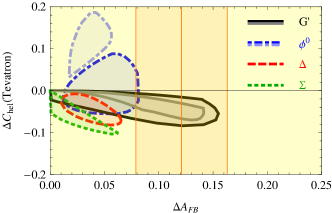
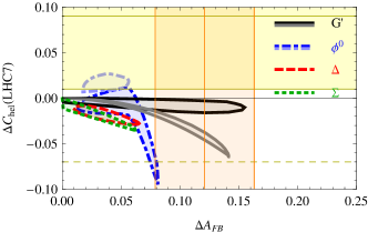
Figure 8: Correlations between the NP contributions to the inclusive FBA at the Tevatron and various spin observables at the 7 TeV LHC (see text for details and definitions). The present experimental results (68%percent6868\% C.L. regions) are shaded in horizontal and vertical bands. For ΔChelΔsubscript𝐶hel\Delta C_{\rm hel} we also show the 95%percent9595\% C.L. contour in thin dashed line. The NP model predictions are determined from the global fit as specified in Sec. IV and are bounded by full (axigluon Gsuperscript𝐺G^{\prime} in the low (mG450less-than-or-similar-tosubscript𝑚𝐺450m_{G}\lesssim 450 GeV in black) and high (mG700greater-than-or-equivalent-tosubscript𝑚𝐺700m_{G}\gtrsim 700 GeV in gray) mass regions), dashed (scalar color triplet ΔΔ\Delta), dotted (scalar color sextet ΣΣ\Sigma) and dot-dashed (neutral component of the scalar isodoublet ϕ0superscriptitalic-ϕ0\phi^{0} in the low (mϕmtless-than-or-similar-tosubscript𝑚italic-ϕsubscript𝑚𝑡m_{\phi}\lesssim m_{t} in darker shade) and high (mϕ>200subscript𝑚italic-ϕ200m_{\phi}>200 GeV in lighter shade) mass region) contours.

Among these, presently the most powerful probe of FBA inspired models is the helicity basis spin correlation as measured recently by ATLAS Aad:2012sm . In particular it already represents a non-trivial constraint for the scalar isodoublet and heavy axigluon models. In the light scalar isodoublet scenario, the large negative deviation in ΔChelΔsubscript𝐶hel\Delta C_{\rm hel} can be traced to sizable non-standard tϕ0u𝑡superscriptitalic-ϕ0𝑢t\to\phi^{0}u decay rate, reducing the experimental tt¯𝑡¯𝑡t\bar{t} reconstruction efficiency (which is then compensated by enhancing the uu¯tt¯𝑢¯𝑢𝑡¯𝑡u\bar{u}\to t\bar{t} cross-section contribution). In term this leads effectively to a reduced gluon fusion component in the tt¯𝑡¯𝑡t\bar{t} cross-section which in this basis contributes sizable positive spin correlations in the SM.

Comparably sensitive (and presently unmeasured) observables are also the opening angle spin correlation coefficient D𝐷D, beamline axis spin correlations (Cbeamsubscript𝐶beamC_{\rm beam}) and helicity axis top polarization (Bhelsubscript𝐵helB_{\rm hel}). 𝒪(5%)𝒪percent5\mathcal{O}(5\%) precision measurements of these quantities could discern among the t𝑡t-channel scalar models. Finally, again we observe that the axigluon (Gsuperscript𝐺G^{\prime}) model (especially in the light mG450less-than-or-similar-tosubscript𝑚𝐺450m_{G}\lesssim 450 GeV region) gives very small contributions to the chosen spin observables at the LHC and will be difficult to probe in this way.

VI Conclusions

We have performed a comprehensive analysis of tt¯𝑡¯𝑡t\bar{t} production phenomenology at the Tevatron and the LHC within effective single NP resonance models addressing the FBA puzzle. We have quantified an inherent tension between the large positive FBA measurements at the Tevatron and precise CA measurements at the LHC (consistent with zero). In particular the later conclusively exclude the Wsuperscript𝑊W^{\prime} and Zsuperscript𝑍Z^{\prime} explanations of the FBA anomaly. Among the considered models, only a color octet axial-vector axigluon state (of mass mG400similar-tosubscript𝑚𝐺400m_{G}\sim 400 GeV or mG1greater-than-or-equivalent-tosubscript𝑚𝐺1m_{G}\gtrsim 1 TeV) can reproduce the central experimentally determined values of the inclusive and the high mtt¯subscript𝑚𝑡¯𝑡m_{t\bar{t}} bin FBA without being in severe conflict with other tt¯𝑡¯𝑡t\bar{t} constraints. In addition, a light scalar isodoublet (mϕmtless-than-or-similar-tosubscript𝑚italic-ϕsubscript𝑚𝑡m_{\phi}\lesssim m_{t}) model predictions can barely reach the one sigma region for the inclusive FBA average, while the central value is in conflict with the LHC cross-section and CA measurements and also the recent top spin correlation measurement by ATLAS. Finally, the scalar color triplet and sextet models are constrained by cross-section and mtt¯subscript𝑚𝑡¯𝑡m_{t\bar{t}} spectrum measurements at the Tevatron. However, given the caveats associated with properly evaluating the contributions of these models (and also the isodoublet model) to the existing experimentally reconstructed mtt¯subscript𝑚𝑡¯𝑡m_{t\bar{t}} spectra (unfolded using SM signal templates), we suggest the experiments at the Tevatron and the LHC perform dedicated studies to settle the issue.

For the favored NP model parameter regions we have derived predictions of (anti)top spin polarization and tt¯𝑡¯𝑡t\bar{t} spin correlation observables at the Tevatron and the LHC. All scalar models addressing the FBA puzzle predict significant deviations in several top spin observables. At the Tevatron the most promising are the (anti)top polarization fractions with respect to the helicity spin quantization axis, which can deviate by more than 20%percent2020\% from their SM predicted values and their measurement could discriminate between scalar isodoublet and color triplet models. At the 777 (and 888) TeV LHC the scalar t(u)𝑡limit-from𝑢t-(u-)channel models predict smaller effects, but helicity axis top spin correlation and polarization measurements at the 510%5percent105-10\% accuracy can yield competitive constraints, as exemplified by the recent ATLAS Aad:2012sm result. On the other hand, a light (mG450less-than-or-similar-tosubscript𝑚𝐺450m_{G}\lesssim 450 GeV) axigluon model predicts very small effects in top spin observables both at the Tevatron and at the LHC, and will be difficult to constrain in this way (much larger effects may be expected only if in addition to the axial component, a vector coupling to qq¯𝑞¯𝑞q\bar{q} pairs is present Falkowski:2011zr ; AFBvsAC ).

While in the present top spin observables’ analysis we have focused on inclusive tt¯𝑡¯𝑡t\bar{t} samples, binned distributions of these quantities in mtt¯subscript𝑚𝑡¯𝑡m_{t\bar{t}} and (anti)top rapidities could further enhance NP effects relative to the SM dominant ggtt¯𝑔𝑔𝑡¯𝑡gg\to t\bar{t} subprocess and help to discriminate between various possible contributions (c.f. Kagan:2011yx ; Arguin:2011xm ; Krohn:2011tw ; Bai:2011uk ; Falkowski:2011zr ; Berger:2012nw for recent proposals along these lines).

Acknowledgements.
J.F.K gratefully acknowledges useful discussions with Gilad Perez and Jure Zupan. The work of S.F. and J.F.K. was supported in part by the Slovenian Research Agency.

Appendix A Partonic Amplitudes

A.1 Parametrization of Standard Model and New Physics Contributions

At the partonic level in the SM the q(p1)q¯(p2)t(k1,st)t¯(k2,st¯)𝑞subscript𝑝1¯𝑞subscript𝑝2𝑡subscript𝑘1subscript𝑠𝑡¯𝑡subscript𝑘2subscript𝑠¯𝑡q(p_{1})\bar{q}(p_{2})\to t(k_{1},s_{t})\bar{t}(k_{2},s_{\bar{t}}) amplitude is given by

iSMqq¯(st,st¯)=igs2sv¯(p2)γμTau(p1)u¯(k1,st)γμTav(k2,st¯),𝑖superscriptsubscript𝑆𝑀𝑞¯𝑞subscript𝑠𝑡subscript𝑠¯𝑡𝑖subscriptsuperscript𝑔2𝑠𝑠¯𝑣subscript𝑝2superscript𝛾𝜇superscript𝑇𝑎𝑢subscript𝑝1¯𝑢subscript𝑘1subscript𝑠𝑡subscript𝛾𝜇superscript𝑇𝑎𝑣subscript𝑘2subscript𝑠¯𝑡i\mathcal{M}_{SM}^{q\bar{q}}(s_{t},s_{\bar{t}})=i\frac{g^{2}_{s}}{s}\bar{v}(p_{2})\gamma^{\mu}T^{a}u(p_{1})\bar{u}(k_{1},s_{t})\gamma_{\mu}T^{a}v(k_{2},s_{\bar{t}})\,, (32)

with s=(p1+p2)2=(k1+k2)2𝑠superscriptsubscript𝑝1subscript𝑝22superscriptsubscript𝑘1subscript𝑘22s=(p_{1}+p_{2})^{2}=(k_{1}+k_{2})^{2}, t=(p1k1)2𝑡superscriptsubscript𝑝1subscript𝑘12t=(p_{1}-k_{1})^{2} and u=(p1k2)2𝑢superscriptsubscript𝑝1subscript𝑘22u=(p_{1}-k_{2})^{2}. Also, gssubscript𝑔𝑠g_{s} denotes the QCD coupling while Tasuperscript𝑇𝑎T^{a} are the Gell-Mann SU(3)𝑆𝑈3SU(3) generator matrices.

Then the unpolarized qq¯𝑞¯𝑞q\bar{q} SM cross section is

dσSMqq¯,unpol.dt=2παs29s2[2(1cos2θ)β2],𝑑superscriptsubscript𝜎𝑆𝑀𝑞¯𝑞unpol𝑑𝑡2𝜋superscriptsubscript𝛼𝑠29superscript𝑠2delimited-[]21superscript2𝜃superscript𝛽2\displaystyle\frac{d\sigma_{SM}^{q\bar{q},\rm unpol.}}{dt}=\frac{2\pi\alpha_{s}^{2}}{9s^{2}}[2-(1-\cos^{2}\theta)\beta^{2}]\,, (33)

while for gg𝑔𝑔gg initial state

dσSMgg,unpol.dt=παs248s2[9(1+β2cos2θ)2](1β2cos2θ)2[1+2β2(1β2)(1cos2θ)β4cos4θ],𝑑superscriptsubscript𝜎𝑆𝑀𝑔𝑔unpol𝑑𝑡𝜋superscriptsubscript𝛼𝑠248superscript𝑠2delimited-[]91superscript𝛽2superscript2𝜃2superscript1superscript𝛽2superscript2𝜃2delimited-[]12superscript𝛽21superscript𝛽21superscript2𝜃superscript𝛽4superscript4𝜃\displaystyle\frac{d\sigma_{SM}^{gg,\rm unpol.}}{dt}=\frac{\pi\alpha_{s}^{2}}{48s^{2}}\frac{[9(1+\beta^{2}\cos^{2}\theta)-2]}{(1-\beta^{2}\cos^{2}\theta)^{2}}[1+2\beta^{2}(1-\beta^{2})(1-\cos^{2}\theta)-\beta^{4}\cos^{4}\theta]\,, (34)

where, as usual, β=14mt2/s𝛽14superscriptsubscript𝑚𝑡2𝑠\beta=\sqrt{1-4m_{t}^{2}/s} and θ𝜃\theta is the scattering angle in the tt¯𝑡¯𝑡t\bar{t} center of mass system.

Since we are also interested in top spin observables, we present also the results for the polarized cross sections. The new physics models which we consider have particles which couple exclusively to quarks and antiquarks and therefore their amplitudes interfere only with the SM qq¯𝑞¯𝑞q\bar{q} parts. The cross sections receive the contribution from the SM, the interference between the SM and the NP, and the NP part only. For all models, denoted by X𝑋X, we thus write

dσSM+Xqq¯,pol.dt=116πs214N2(|SMqq¯,pol.|2+|SMXpol.|2+|Xpol.|2),𝑑superscriptsubscript𝜎𝑆𝑀𝑋𝑞¯𝑞pol𝑑𝑡116𝜋superscript𝑠214superscript𝑁2superscriptsubscriptsuperscript𝑞¯𝑞pol𝑆𝑀2superscriptsubscriptsuperscriptpol𝑆𝑀𝑋2superscriptsubscriptsuperscriptpol𝑋2\displaystyle\frac{d\sigma_{SM+X}^{q\bar{q},\rm pol.}}{dt}=\frac{1}{16\pi s^{2}}\frac{1}{4N^{2}}(|\mathcal{M}^{q\bar{q},\rm pol.}_{SM}|^{2}+|\mathcal{M}^{\rm pol.}_{SM*X}|^{2}+|\mathcal{M}^{\rm pol.}_{X}|^{2})\,, (35)

where N=3𝑁3N=3 is the number of colors each square of the polarized amplitudes can be written as

|pol.|2superscriptsuperscriptpol2\displaystyle|\mathcal{M}^{\rm pol.}|^{2} =\displaystyle= a+bμtstμ+bμt¯st¯μ+cμνstμst¯ν,𝑎subscriptsuperscript𝑏𝑡𝜇superscriptsubscript𝑠𝑡𝜇subscriptsuperscript𝑏¯𝑡𝜇superscriptsubscript𝑠¯𝑡𝜇subscript𝑐𝜇𝜈superscriptsubscript𝑠𝑡𝜇superscriptsubscript𝑠¯𝑡𝜈\displaystyle a+b^{t}_{\mu}s_{t}^{\mu}+b^{\bar{t}}_{\mu}s_{\bar{t}}^{\mu}+c_{\mu\nu}s_{t}^{\mu}s_{\bar{t}}^{\nu}\,, (36)

and further

bμtstμsubscriptsuperscript𝑏𝑡𝜇superscriptsubscript𝑠𝑡𝜇\displaystyle b^{t}_{\mu}s_{t}^{\mu} =\displaystyle= b1t(p1st)+b2t(p2st),subscriptsuperscript𝑏𝑡1subscript𝑝1subscript𝑠𝑡subscriptsuperscript𝑏𝑡2subscript𝑝2subscript𝑠𝑡\displaystyle b^{t}_{1}(p_{1}\cdot s_{t})+b^{t}_{2}(p_{2}\cdot s_{t})\,, (37)
bμt¯st¯μsubscriptsuperscript𝑏¯𝑡𝜇superscriptsubscript𝑠¯𝑡𝜇\displaystyle b^{\bar{t}}_{\mu}s_{\bar{t}}^{\mu} =\displaystyle= b1t¯(p1st¯)+b2t¯(p2st¯),subscriptsuperscript𝑏¯𝑡1subscript𝑝1subscript𝑠¯𝑡subscriptsuperscript𝑏¯𝑡2subscript𝑝2subscript𝑠¯𝑡\displaystyle b^{\bar{t}}_{1}(p_{1}\cdot s_{\bar{t}})+b^{\bar{t}}_{2}(p_{2}\cdot s_{\bar{t}})\,, (38)
cμνstμst¯νsubscript𝑐𝜇𝜈superscriptsubscript𝑠𝑡𝜇superscriptsubscript𝑠¯𝑡𝜈\displaystyle c_{\mu\nu}s_{t}^{\mu}s_{\bar{t}}^{\nu} =\displaystyle= c(stst¯)+d[(p1st)(p1st¯)+(p2st)(p2st¯)],𝑐subscript𝑠𝑡subscript𝑠¯𝑡𝑑delimited-[]subscript𝑝1subscript𝑠𝑡subscript𝑝1subscript𝑠¯𝑡subscript𝑝2subscript𝑠𝑡subscript𝑝2subscript𝑠¯𝑡\displaystyle c(s_{t}\cdot s_{\bar{t}})+d[(p_{1}\cdot s_{t})(p_{1}\cdot s_{\bar{t}})+(p_{2}\cdot s_{t})(p_{2}\cdot s_{\bar{t}})]\,, (39)
+e(p1st)(p2st¯)+f(p2st)(p1st¯).𝑒subscript𝑝1subscript𝑠𝑡subscript𝑝2subscript𝑠¯𝑡𝑓subscript𝑝2subscript𝑠𝑡subscript𝑝1subscript𝑠¯𝑡\displaystyle+e(p_{1}\cdot s_{t})(p_{2}\cdot s_{\bar{t}})+f(p_{2}\cdot s_{t})(p_{1}\cdot s_{\bar{t}})\,.

Due to the CP invariance in our models, b1t¯=b2tsuperscriptsubscript𝑏1¯𝑡superscriptsubscript𝑏2𝑡b_{1}^{\bar{t}}=-b_{2}^{t} and b2t¯=b1tsuperscriptsubscript𝑏2¯𝑡superscriptsubscript𝑏1𝑡b_{2}^{\bar{t}}=-b_{1}^{t}.

The spin coefficients for the polarized qq¯𝑞¯𝑞q\bar{q} squared amplitude in the SM are as follows:

aSMqq¯superscriptsubscript𝑎𝑆𝑀𝑞¯𝑞\displaystyle a_{SM}^{q\bar{q}} =\displaystyle= CSMqq¯[2β2(1z2)],superscriptsubscript𝐶𝑆𝑀𝑞¯𝑞delimited-[]2superscript𝛽21superscript𝑧2\displaystyle C_{SM}^{q\bar{q}}\left[2-\beta^{2}(1-z^{2})\right]\,,
cSMqq¯superscriptsubscript𝑐𝑆𝑀𝑞¯𝑞\displaystyle c_{SM}^{q\bar{q}} =\displaystyle= CSMqq¯[β2(1z2)],superscriptsubscript𝐶𝑆𝑀𝑞¯𝑞delimited-[]superscript𝛽21superscript𝑧2\displaystyle C_{SM}^{q\bar{q}}\left[\beta^{2}(1-z^{2})\right]\,,
eSMqq¯superscriptsubscript𝑒𝑆𝑀𝑞¯𝑞\displaystyle e_{SM}^{q\bar{q}} =\displaystyle= CSMqq¯[4s(1+βz)],superscriptsubscript𝐶𝑆𝑀𝑞¯𝑞delimited-[]4𝑠1𝛽𝑧\displaystyle C_{SM}^{q\bar{q}}\left[-\frac{4}{s}(1+\beta z)\right]\,,
fSMqq¯superscriptsubscript𝑓𝑆𝑀𝑞¯𝑞\displaystyle f_{SM}^{q\bar{q}} =\displaystyle= CSMqq¯[4s(1βz)],superscriptsubscript𝐶𝑆𝑀𝑞¯𝑞delimited-[]4𝑠1𝛽𝑧\displaystyle C_{SM}^{q\bar{q}}\left[-\frac{4}{s}(1-\beta z)\right]\,, (40)

where CSMqq¯=16π2αs2(N21)superscriptsubscript𝐶𝑆𝑀𝑞¯𝑞16superscript𝜋2superscriptsubscript𝛼𝑠2superscript𝑁21C_{SM}^{q\bar{q}}=16\pi^{2}\alpha_{s}^{2}(N^{2}-1) and z=cosθ𝑧𝜃z=\cos\theta. All other coefficients are zero. On the other hand, the polarized SM gg𝑔𝑔gg-cross section has the form

dσSMgg,pol.dt=116πs214(N21)2|SMgg,pol.|2,𝑑superscriptsubscript𝜎𝑆𝑀𝑔𝑔pol𝑑𝑡116𝜋superscript𝑠214superscriptsuperscript𝑁212superscriptsubscriptsuperscript𝑔𝑔pol𝑆𝑀2\displaystyle\frac{d\sigma_{SM}^{gg,\rm pol.}}{dt}=\frac{1}{16\pi s^{2}}\frac{1}{4(N^{2}-1)^{2}}|\mathcal{M}^{gg,\rm pol.}_{SM}|^{2}\,, (41)

and |MSMgg,pol.|2superscriptsubscriptsuperscript𝑀𝑔𝑔pol𝑆𝑀2|M^{gg,\rm pol.}_{SM}|^{2} can be written with the help of

aSMggsuperscriptsubscript𝑎𝑆𝑀𝑔𝑔\displaystyle a_{SM}^{gg} =\displaystyle= CSMgg[1+2β2(1z2)(22z2+z4)β4],superscriptsubscript𝐶𝑆𝑀𝑔𝑔delimited-[]12superscript𝛽21superscript𝑧222superscript𝑧2superscript𝑧4superscript𝛽4\displaystyle C_{SM}^{gg}\left[1+2\beta^{2}(1-z^{2})-(2-2z^{2}+z^{4})\beta^{4}\right]\,,
cSMggsuperscriptsubscript𝑐𝑆𝑀𝑔𝑔\displaystyle c_{SM}^{gg} =\displaystyle= CSMgg[12β2+(22z2+z4)β4],superscriptsubscript𝐶𝑆𝑀𝑔𝑔delimited-[]12superscript𝛽222superscript𝑧2superscript𝑧4superscript𝛽4\displaystyle C_{SM}^{gg}\left[1-2\beta^{2}+(2-2z^{2}+z^{4})\beta^{4}\right]\,,
eSMggsuperscriptsubscript𝑒𝑆𝑀𝑔𝑔\displaystyle e_{SM}^{gg} =\displaystyle= CSMgg[4sβ2(1+βz)(1z2)],superscriptsubscript𝐶𝑆𝑀𝑔𝑔delimited-[]4𝑠superscript𝛽21𝛽𝑧1superscript𝑧2\displaystyle C_{SM}^{gg}\left[-\frac{4}{s}\beta^{2}(1+\beta z)(1-z^{2})\right]\,,
fSMggsuperscriptsubscript𝑓𝑆𝑀𝑔𝑔\displaystyle f_{SM}^{gg} =\displaystyle= CSMgg[4sβ2(1βz)(1z2)],superscriptsubscript𝐶𝑆𝑀𝑔𝑔delimited-[]4𝑠superscript𝛽21𝛽𝑧1superscript𝑧2\displaystyle C_{SM}^{gg}\left[-\frac{4}{s}\beta^{2}(1-\beta z)(1-z^{2})\right]\,, (42)

where CSMqq=32π2αs2(N2(1+β2z2)2)(1β2z2)2(N21)Nsuperscriptsubscript𝐶𝑆𝑀𝑞𝑞32superscript𝜋2superscriptsubscript𝛼𝑠2superscript𝑁21superscript𝛽2superscript𝑧22superscript1superscript𝛽2superscript𝑧22superscript𝑁21𝑁C_{SM}^{qq}=32\pi^{2}\alpha_{s}^{2}\frac{(N^{2}(1+\beta^{2}z^{2})-2)}{(1-\beta^{2}z^{2})^{2}}\frac{(N^{2}-1)}{N}. These expressions can be also found in Secs. 2.1.1. and 2.1.2 of spinSM .

A.2 New Physics Models

A.2.1 Axigluon

The relevant interaction part of the Lagrangian describing new physics in the tt¯𝑡¯𝑡t\bar{t} production due to s-channel axigluon Gsuperscript𝐺{G^{\prime}} exchange is given by ,

Gint.=q¯(gVqgAqγ5)/Gqt¯(gVtgAtγ5)/Gt,subscriptsuperscriptintsuperscript𝐺¯𝑞superscriptsubscript𝑔𝑉𝑞superscriptsubscript𝑔𝐴𝑞subscript𝛾5superscript𝐺𝑞¯𝑡superscriptsubscript𝑔𝑉𝑡superscriptsubscript𝑔𝐴𝑡subscript𝛾5superscript𝐺𝑡{\cal L}^{\rm int.}_{G^{\prime}}=-\bar{q}(g_{V}^{q}-g_{A}^{q}\gamma_{5}){/\!\!\!G^{\prime}}q-\bar{t}(g_{V}^{t}-g_{A}^{t}\gamma_{5}){/\!\!\!G^{\prime}}t\,, (43)

The new qq¯tt¯𝑞¯𝑞𝑡¯𝑡q\bar{q}\to t\bar{t} amplitude is then

iG=iTijaTkla1smG2+imGΓGv¯i(p2)γμ(gVq+gAqγ5)uj(p1)u¯k(k1,st)γμ(gVt+gAtγ5)vl(k2,st¯),𝑖subscriptsuperscript𝐺𝑖subscriptsuperscript𝑇𝑎𝑖𝑗subscriptsuperscript𝑇𝑎𝑘𝑙1𝑠superscriptsubscript𝑚𝐺2𝑖subscript𝑚𝐺subscriptΓ𝐺superscript¯𝑣𝑖subscript𝑝2superscript𝛾𝜇superscriptsubscript𝑔𝑉𝑞superscriptsubscript𝑔𝐴𝑞subscript𝛾5superscript𝑢𝑗subscript𝑝1superscript¯𝑢𝑘subscript𝑘1subscript𝑠𝑡subscript𝛾𝜇superscriptsubscript𝑔𝑉𝑡superscriptsubscript𝑔𝐴𝑡subscript𝛾5superscript𝑣𝑙subscript𝑘2subscript𝑠¯𝑡i\mathcal{M}_{G^{\prime}}=iT^{a}_{ij}T^{a}_{kl}\frac{1}{s-m_{G}^{2}+im_{G}\Gamma_{G}}\bar{v}^{i}(p_{2})\gamma^{\mu}(g_{V}^{q}+g_{A}^{q}\gamma_{5})u^{j}(p_{1})\bar{u}^{k}(k_{1},s_{t})\gamma_{\mu}(g_{V}^{t}+g_{A}^{t}\gamma_{5})v^{l}(k_{2},s_{\bar{t}})\,, (44)

where mGsubscript𝑚𝐺m_{G} is the axigluon mass and ΓGsubscriptΓ𝐺\Gamma_{G} is the manually introduced axigluon width. The resulting unpolarized qq¯tt¯𝑞¯𝑞𝑡¯𝑡q\bar{q}\to t\bar{t} cross section is of the form axig2

dσSM+Gqq¯,unpol.dt𝑑superscriptsubscript𝜎𝑆𝑀superscript𝐺𝑞¯𝑞unpol𝑑𝑡\displaystyle\frac{d\sigma_{SM+G^{\prime}}^{q\bar{q},\rm unpol.}}{dt} =\displaystyle= dσSMqq¯,unpol.dt+2π9s2αs2{s(smG2)(smG2)2+ΓG2mG22(g¯Vqg¯Vt(1+β2z2+4mt2/s)+2g¯Aqg¯Atβz)\displaystyle\frac{d\sigma_{SM}^{q\bar{q},\rm unpol.}}{dt}+\frac{2\pi}{9s^{2}}\alpha_{s}^{2}\Bigg{\{}\frac{s(s-m_{G}^{2})}{(s-m_{G}^{2})^{2}+\Gamma_{G}^{2}m_{G}^{2}}2\left(\bar{g}_{V}^{q}\bar{g}_{V}^{t}(1+\beta^{2}z^{2}+4m_{t}^{2}/s)+2\bar{g}_{A}^{q}\bar{g}_{A}^{t}\beta z\right) (45)
+\displaystyle+ s2(smG2)2+ΓG2mG2[((g¯Vq)2+(g¯Ag)2)((g¯Vt)2(1+β2z2+4mt2/s)\displaystyle\frac{s^{2}}{(s-m_{G}^{2})^{2}+\Gamma_{G}^{2}m_{G}^{2}}\left[\left((\bar{g}_{V}^{q})^{2}+(\bar{g}_{A}^{g})^{2}\right)\left((\bar{g}_{V}^{t})^{2}(1+\beta^{2}z^{2}+4m_{t}^{2}/s)\right.\right.
+(g¯At)2(1+β2z24mt2/s)+8βzg¯Vqg¯Vtg¯Aqg¯At)]},\displaystyle\left.\left.+(\bar{g}_{A}^{t})^{2}(1+\beta^{2}z^{2}-4m_{t}^{2}/s)+8\beta z\bar{g}_{V}^{q}\bar{g}_{V}^{t}\bar{g}_{A}^{q}\bar{g}_{A}^{t}\right)\right]\Bigg{\}}\,,

where now g¯V,Aq,t=gV,Aq,t/gssuperscriptsubscript¯𝑔𝑉𝐴𝑞𝑡superscriptsubscript𝑔𝑉𝐴𝑞𝑡subscript𝑔𝑠\bar{g}_{V,A}^{q,t}=g_{V,A}^{q,t}/g_{s}.

The polarized parts are given (for gVq=gVt=0superscriptsubscript𝑔𝑉𝑞superscriptsubscript𝑔𝑉𝑡0g_{V}^{q}=g_{V}^{t}=0) by the following expressions, eq. (39):

aSMGsubscript𝑎𝑆𝑀superscript𝐺\displaystyle a_{SM*G^{\prime}} =\displaystyle= CSMG[4βz],subscript𝐶𝑆𝑀superscript𝐺delimited-[]4𝛽𝑧\displaystyle C_{SM*G^{\prime}}[4\beta z]\,,
eSMGsubscript𝑒𝑆𝑀superscript𝐺\displaystyle e_{SM*G^{\prime}} =\displaystyle= CSMG[16mt2s2],subscript𝐶𝑆𝑀superscript𝐺delimited-[]16superscriptsubscript𝑚𝑡2superscript𝑠2\displaystyle C_{SM*G^{\prime}}\left[\frac{16m_{t}^{2}}{s^{2}}\right]\,,
fSMGsubscript𝑓𝑆𝑀superscript𝐺\displaystyle f_{SM*G^{\prime}} =\displaystyle= CSMG[16mt2s2],subscript𝐶𝑆𝑀superscript𝐺delimited-[]16superscriptsubscript𝑚𝑡2superscript𝑠2\displaystyle C_{SM*G^{\prime}}\left[\frac{-16m_{t}^{2}}{s^{2}}\right]\,, (46)

and

aGsubscript𝑎superscript𝐺\displaystyle a_{G^{\prime}} =\displaystyle= CG[14mt2/s+β2z2],subscript𝐶superscript𝐺delimited-[]14superscriptsubscript𝑚𝑡2𝑠superscript𝛽2superscript𝑧2\displaystyle C_{G^{\prime}}[1-4m_{t}^{2}/s+\beta^{2}z^{2}]\,,
cGsubscript𝑐superscript𝐺\displaystyle c_{G^{\prime}} =\displaystyle= CG[1+4mt2/s+β2z2],subscript𝐶superscript𝐺delimited-[]14superscriptsubscript𝑚𝑡2𝑠superscript𝛽2superscript𝑧2\displaystyle C_{G^{\prime}}[-1+4m_{t}^{2}/s+\beta^{2}z^{2}]\,,
eGsubscript𝑒superscript𝐺\displaystyle e_{G^{\prime}} =\displaystyle= CG[4s(14mt2/s+βz)],subscript𝐶superscript𝐺delimited-[]4𝑠14superscriptsubscript𝑚𝑡2𝑠𝛽𝑧\displaystyle C_{G^{\prime}}\left[\frac{4}{s}(1-4m_{t}^{2}/s+\beta z)\right]\,,
fGsubscript𝑓superscript𝐺\displaystyle f_{G^{\prime}} =\displaystyle= CG[4s(1+4mt2/s+βz)],subscript𝐶superscript𝐺delimited-[]4𝑠14superscriptsubscript𝑚𝑡2𝑠𝛽𝑧\displaystyle C_{G^{\prime}}\left[\frac{4}{s}(-1+4m_{t}^{2}/s+\beta z)\right]\,, (47)

where

CSMGsubscript𝐶𝑆𝑀superscript𝐺\displaystyle C_{SM*G^{\prime}} =\displaystyle= 16π2αs2(N21)gAqg¯Ats(smG2)(smG2)2+ΓG2mG2,16superscript𝜋2superscriptsubscript𝛼𝑠2superscript𝑁21superscriptsubscript𝑔𝐴𝑞superscriptsubscript¯𝑔𝐴𝑡𝑠𝑠superscriptsubscript𝑚𝐺2superscript𝑠superscriptsubscript𝑚𝐺22superscriptsubscriptΓ𝐺2superscriptsubscript𝑚𝐺2\displaystyle 16\pi^{2}\alpha_{s}^{2}(N^{2}-1)\frac{g_{A}^{q}\bar{g}_{A}^{t}\,s(s-m_{G}^{2})}{(s-m_{G}^{2})^{2}+\Gamma_{G}^{2}m_{G}^{2}}\,,
CGsubscript𝐶superscript𝐺\displaystyle C_{G^{\prime}} =\displaystyle= 16π2αs2(N21)(g¯Aq)2(g¯At)2s2(smG2)2+ΓG2mG2.16superscript𝜋2superscriptsubscript𝛼𝑠2superscript𝑁21superscriptsuperscriptsubscript¯𝑔𝐴𝑞2superscriptsuperscriptsubscript¯𝑔𝐴𝑡2superscript𝑠2superscript𝑠superscriptsubscript𝑚𝐺22superscriptsubscriptΓ𝐺2superscriptsubscript𝑚𝐺2\displaystyle 16\pi^{2}\alpha_{s}^{2}(N^{2}-1)\frac{(\bar{g}_{A}^{q})^{2}(\bar{g}_{A}^{t})^{2}\,s^{2}}{(s-m_{G}^{2})^{2}+\Gamma_{G}^{2}m_{G}^{2}}\,. (48)

Other coefficients in (39) are vanishing.

A.2.2 Zsuperscript𝑍Z^{\prime} and Wsuperscript𝑊W^{\prime}

The interactions of the heavy weak bosons Zsuperscript𝑍Z^{\prime} and Wsuperscript𝑊W^{\prime} contributing in the t-channel of the tt¯𝑡¯𝑡t\bar{t} production are given by the following Lagrangians:

Zint.=u¯γμ(fLZPL+fRZPR)tZ+h.c.,formulae-sequencesubscriptsuperscriptintsuperscript𝑍¯𝑢subscript𝛾𝜇superscriptsubscript𝑓𝐿superscript𝑍subscript𝑃𝐿superscriptsubscript𝑓𝑅superscript𝑍subscript𝑃𝑅𝑡superscript𝑍hc{\cal L}^{\rm int.}_{Z^{\prime}}=-\bar{u}\gamma_{\mu}(f_{L}^{Z^{\prime}}P_{L}+f_{R}^{Z^{\prime}}P_{R})tZ^{\prime}+\rm h.c.\,, (49)
Wint.=d¯γμ(fLWPL+fRWPR)tW+h.c..formulae-sequencesubscriptsuperscriptintsuperscript𝑊¯𝑑subscript𝛾𝜇superscriptsubscript𝑓𝐿superscript𝑊subscript𝑃𝐿superscriptsubscript𝑓𝑅superscript𝑊subscript𝑃𝑅𝑡superscript𝑊hc{\cal L}^{\rm int.}_{W^{\prime}}=-\bar{d}\gamma_{\mu}(f_{L}^{W^{\prime}}P_{L}+f_{R}^{W^{\prime}}P_{R})tW^{\prime}+\rm h.c.\,. (50)

The relevant amplitude induced by the new physics contributions is

iZ=iu¯(k1,st)γμ(fLZPL+fRZPR)u(p1)(gμνtmZ2+tμtνmZ2(tmZ2))v¯(p2)γν(fLZPL+fRZPR)v(k2,st¯)𝑖subscriptsuperscript𝑍𝑖¯𝑢subscript𝑘1subscript𝑠𝑡superscript𝛾𝜇superscriptsubscript𝑓𝐿superscript𝑍subscript𝑃𝐿superscriptsubscript𝑓𝑅superscript𝑍subscript𝑃𝑅𝑢subscript𝑝1superscript𝑔𝜇𝜈𝑡superscriptsubscript𝑚superscript𝑍2superscript𝑡𝜇superscript𝑡𝜈superscriptsubscript𝑚superscript𝑍2𝑡superscriptsubscript𝑚superscript𝑍2¯𝑣subscript𝑝2superscript𝛾𝜈superscriptsubscript𝑓𝐿superscript𝑍subscript𝑃𝐿superscriptsubscript𝑓𝑅superscript𝑍subscript𝑃𝑅𝑣subscript𝑘2subscript𝑠¯𝑡\displaystyle i\mathcal{M}_{Z^{\prime}}=i\bar{u}(k_{1},s_{t})\gamma^{\mu}(f_{L}^{Z^{\prime}}P_{L}+f_{R}^{Z^{\prime}}P_{R})u(p_{1})\left(-\frac{g^{\mu\nu}}{t-m_{Z^{\prime}}^{2}}+\frac{t^{\mu}t^{\nu}}{m_{Z^{\prime}}^{2}(t-m_{Z^{\prime}}^{2})}\right)\bar{v}(p_{2})\gamma^{\nu}(f_{L}^{Z^{\prime}}P_{L}+f_{R}^{Z^{\prime}}P_{R})v(k_{2},s_{\bar{t}})

where tμ=(p1k1)μsuperscript𝑡𝜇superscriptsubscript𝑝1subscript𝑘1𝜇t^{\mu}=(p_{1}-k_{1})^{\mu} , and similarly for the interaction with the Wsuperscript𝑊W^{\prime}, by the exchange ZWsuperscript𝑍superscript𝑊Z^{\prime}\to W^{\prime} and ud𝑢𝑑u\to d. Then

dσSM+Zuu¯,unpol.dt𝑑subscriptsuperscript𝜎𝑢¯𝑢unpol𝑆𝑀superscript𝑍𝑑𝑡\displaystyle\frac{d\sigma^{u\bar{u},\rm unpol.}_{SM+Z^{\prime}}}{dt} =\displaystyle= dσSMuu¯,unpol.dt+αs9s3(fLZ)2+(fRZ)2tmZ2{2ut2+2smt2+mt2mZ2(tt2+mt2s)}𝑑superscriptsubscript𝜎𝑆𝑀𝑢¯𝑢unpol𝑑𝑡subscript𝛼𝑠9superscript𝑠3superscriptsuperscriptsubscript𝑓𝐿superscript𝑍2superscriptsuperscriptsubscript𝑓𝑅superscript𝑍2𝑡superscriptsubscript𝑚superscript𝑍22superscriptsubscript𝑢𝑡22𝑠superscriptsubscript𝑚𝑡2superscriptsubscript𝑚𝑡2superscriptsubscript𝑚superscript𝑍2superscriptsubscript𝑡𝑡2superscriptsubscript𝑚𝑡2𝑠\displaystyle\frac{d\sigma_{SM}^{u\bar{u},\rm unpol.}}{dt}+\frac{\alpha_{s}}{9s^{3}}\frac{(f_{L}^{Z^{\prime}})^{2}+(f_{R}^{Z^{\prime}})^{2}}{t-m_{Z^{\prime}}^{2}}\{2u_{t}^{2}+2sm_{t}^{2}+\frac{m_{t}^{2}}{m_{Z^{\prime}}^{2}}(t_{t}^{2}+m_{t}^{2}s)\} (52)
+\displaystyle+ 116πs21(tmZ2)2{((fLZ)4+(fRZ)4)ut2+2(fLZ)2(fRZ)2s(s2mt2)\displaystyle\frac{1}{16\pi s^{2}}\frac{1}{(t-m_{Z^{\prime}}^{2})^{2}}\left\{\left((f_{L}^{Z^{\prime}})^{4}+(f_{R}^{Z^{\prime}})^{4}\right)u_{t}^{2}+2(f_{L}^{Z^{\prime}})^{2}(f_{R}^{Z^{\prime}})^{2}s(s-2m_{t}^{2})\right.
+mt44mZ4((fLZ)2+(fRZ)2)2(tt2+4smZ2)},\displaystyle\left.+\frac{m_{t}^{4}}{4m_{Z^{\prime}}^{4}}\left((f_{L}^{Z^{\prime}})^{2}+(f_{R}^{Z^{\prime}})^{2}\right)^{2}(t_{t}^{2}+4sm_{Z^{\prime}}^{2})\right\}\,,

where ut=s(1+βz)/2,tt=s(1βz)/2formulae-sequencesubscript𝑢𝑡𝑠1𝛽𝑧2subscript𝑡𝑡𝑠1𝛽𝑧2u_{t}=s(1+\beta z)/2,t_{t}=s(1-\beta z)/2.

The polarized case we consider only the right-handed couplings and the non-vanishing spin coefficients in (39) are

aSMZsubscript𝑎𝑆𝑀superscript𝑍\displaystyle a_{SM*Z^{\prime}} =\displaystyle= CSMZ[4mt2+s(1+βz)2+mt22mZ2(4mt2+s(1βz)2)],subscript𝐶𝑆𝑀superscript𝑍delimited-[]4superscriptsubscript𝑚𝑡2𝑠superscript1𝛽𝑧2superscriptsubscript𝑚𝑡22superscriptsubscript𝑚superscript𝑍24superscriptsubscript𝑚𝑡2𝑠superscript1𝛽𝑧2\displaystyle C_{SM*Z^{\prime}}\left[4m_{t}^{2}+s(1+\beta z)^{2}+\frac{m_{t}^{2}}{2m_{Z^{\prime}}^{2}}(4m_{t}^{2}+s(1-\beta z)^{2})\right]\,,
cSMZsubscript𝑐𝑆𝑀superscript𝑍\displaystyle c_{SM*Z^{\prime}} =\displaystyle= CSMZ[4mt2+s(1β2z2)mt22mZ2(4mt2s(1β2z2))],subscript𝐶𝑆𝑀superscript𝑍delimited-[]4superscriptsubscript𝑚𝑡2𝑠1superscript𝛽2superscript𝑧2superscriptsubscript𝑚𝑡22superscriptsubscript𝑚superscript𝑍24superscriptsubscript𝑚𝑡2𝑠1superscript𝛽2superscript𝑧2\displaystyle C_{SM*Z^{\prime}}\left[-4m_{t}^{2}+s(1-\beta^{2}z^{2})-\frac{m_{t}^{2}}{2m_{Z^{\prime}}^{2}}(4m_{t}^{2}-s(1-\beta^{2}z^{2}))\right]\,,
eSMZsubscript𝑒𝑆𝑀superscript𝑍\displaystyle e_{SM*Z^{\prime}} =\displaystyle= CSMZ[4s(2mt2s(1+βz)mt22mZ2(2mt2+s(1+βz)))],subscript𝐶𝑆𝑀superscript𝑍delimited-[]4𝑠2superscriptsubscript𝑚𝑡2𝑠1𝛽𝑧superscriptsubscript𝑚𝑡22superscriptsubscript𝑚superscript𝑍22superscriptsubscript𝑚𝑡2𝑠1𝛽𝑧\displaystyle C_{SM*Z^{\prime}}\left[\frac{4}{s}\left(2m_{t}^{2}-s(1+\beta z)-\frac{m_{t}^{2}}{2m_{Z^{\prime}}^{2}}(2m_{t}^{2}+s(1+\beta z))\right)\right]\,,
fSMZsubscript𝑓𝑆𝑀superscript𝑍\displaystyle f_{SM*Z^{\prime}} =\displaystyle= CSMZ[4s(2mt2+s(1βz)mt22mZ2(2mt2s(1βz)))],subscript𝐶𝑆𝑀superscript𝑍delimited-[]4𝑠2superscriptsubscript𝑚𝑡2𝑠1𝛽𝑧superscriptsubscript𝑚𝑡22superscriptsubscript𝑚superscript𝑍22superscriptsubscript𝑚𝑡2𝑠1𝛽𝑧\displaystyle C_{SM*Z^{\prime}}\left[\frac{-4}{s}\left(2m_{t}^{2}+s(1-\beta z)-\frac{m_{t}^{2}}{2m_{Z^{\prime}}^{2}}(2m_{t}^{2}-s(1-\beta z))\right)\right]\,,
(b1t)SMZsubscriptsuperscriptsubscript𝑏1𝑡𝑆𝑀superscript𝑍\displaystyle(b_{1}^{t})_{SM*Z^{\prime}} =\displaystyle= CSMZ[2mt(1+βz+mt22mZ2(3βz))],subscript𝐶𝑆𝑀superscript𝑍delimited-[]2subscript𝑚𝑡1𝛽𝑧superscriptsubscript𝑚𝑡22superscriptsubscript𝑚superscript𝑍23𝛽𝑧\displaystyle C_{SM*Z^{\prime}}\left[-2m_{t}\left(1+\beta z+\frac{m_{t}^{2}}{2m_{Z^{\prime}}^{2}}(3-\beta z)\right)\right]\,,
(b2t)SMZsubscriptsuperscriptsubscript𝑏2𝑡𝑆𝑀superscript𝑍\displaystyle(b_{2}^{t})_{SM*Z^{\prime}} =\displaystyle= CSMZ[2mt(3+βz+mt22mZ2(1βz))],subscript𝐶𝑆𝑀superscript𝑍delimited-[]2subscript𝑚𝑡3𝛽𝑧superscriptsubscript𝑚𝑡22superscriptsubscript𝑚superscript𝑍21𝛽𝑧\displaystyle C_{SM*Z^{\prime}}\left[-2m_{t}\left(3+\beta z+\frac{m_{t}^{2}}{2m_{Z^{\prime}}^{2}}(1-\beta z)\right)\right]\,,

and

aZsubscript𝑎superscript𝑍\displaystyle a_{Z^{\prime}} =\displaystyle= CZ[s(1+βz)2+4mt4mZ2+mt44mZ4s(1βz)2],subscript𝐶superscript𝑍delimited-[]𝑠superscript1𝛽𝑧24superscriptsubscript𝑚𝑡4superscriptsubscript𝑚superscript𝑍2superscriptsubscript𝑚𝑡44superscriptsubscript𝑚superscript𝑍4𝑠superscript1𝛽𝑧2\displaystyle C_{Z^{\prime}}\left[s(1+\beta z)^{2}+4\frac{m_{t}^{4}}{m_{Z^{\prime}}^{2}}+\frac{m_{t}^{4}}{4m_{Z^{\prime}}^{4}}s(1-\beta z)^{2}\right]\,,
cZsubscript𝑐superscript𝑍\displaystyle c_{Z^{\prime}} =\displaystyle= CZ[mt2mZ2(s(1β2z2)4mt2)],subscript𝐶superscript𝑍delimited-[]superscriptsubscript𝑚𝑡2superscriptsubscript𝑚superscript𝑍2𝑠1superscript𝛽2superscript𝑧24superscriptsubscript𝑚𝑡2\displaystyle C_{Z^{\prime}}\left[\frac{m_{t}^{2}}{m_{Z^{\prime}}^{2}}\left(s(1-\beta^{2}z^{2})-4m_{t}^{2}\right)\right]\,,
eZsubscript𝑒superscript𝑍\displaystyle e_{Z^{\prime}} =\displaystyle= CZ[4smt2mZ2(2mt2s(1+βz)mt4mZ2)],subscript𝐶superscript𝑍delimited-[]4𝑠superscriptsubscript𝑚𝑡2superscriptsubscript𝑚superscript𝑍22superscriptsubscript𝑚𝑡2𝑠1𝛽𝑧superscriptsubscript𝑚𝑡4superscriptsubscript𝑚superscript𝑍2\displaystyle C_{Z^{\prime}}\left[\frac{4}{s}\frac{m_{t}^{2}}{m_{Z^{\prime}}^{2}}\left(2m_{t}^{2}-s(1+\beta z)-\frac{m_{t}^{4}}{m_{Z^{\prime}}^{2}}\right)\right]\,,
fZsubscript𝑓superscript𝑍\displaystyle f_{Z^{\prime}} =\displaystyle= CZ[4smt2mZ2(2mt2s(1βz)4mZ2)],subscript𝐶superscript𝑍delimited-[]4𝑠superscriptsubscript𝑚𝑡2superscriptsubscript𝑚superscript𝑍22superscriptsubscript𝑚𝑡2𝑠1𝛽𝑧4superscriptsubscript𝑚superscript𝑍2\displaystyle C_{Z^{\prime}}\left[\frac{4}{s}\frac{m_{t}^{2}}{m_{Z^{\prime}}^{2}}\left(2m_{t}^{2}-s(1-\beta z)-4m_{Z^{\prime}}^{2}\right)\right]\,,
(b1t)Zsubscriptsuperscriptsubscript𝑏1𝑡superscript𝑍\displaystyle(b_{1}^{t})_{Z^{\prime}} =\displaystyle= CZ[2mtmt2mZ2((1+βz)+mt22mZ2(1βz))],subscript𝐶superscript𝑍delimited-[]2subscript𝑚𝑡superscriptsubscript𝑚𝑡2superscriptsubscript𝑚superscript𝑍21𝛽𝑧superscriptsubscript𝑚𝑡22superscriptsubscript𝑚superscript𝑍21𝛽𝑧\displaystyle C_{Z^{\prime}}\left[-2m_{t}\frac{m_{t}^{2}}{m_{Z^{\prime}}^{2}}\left((1+\beta z)+\frac{m_{t}^{2}}{2m_{Z^{\prime}}^{2}}(1-\beta z)\right)\right]\,,
(b2t)Zsubscriptsuperscriptsubscript𝑏2𝑡superscript𝑍\displaystyle(b_{2}^{t})_{Z^{\prime}} =\displaystyle= CZ[4mt((1+βz)+mt22mZ2(1βz))],subscript𝐶superscript𝑍delimited-[]4subscript𝑚𝑡1𝛽𝑧superscriptsubscript𝑚𝑡22superscriptsubscript𝑚superscript𝑍21𝛽𝑧\displaystyle C_{Z^{\prime}}\left[-4m_{t}\left((1+\beta z)+\frac{m_{t}^{2}}{2m_{Z^{\prime}}^{2}}(1-\beta z)\right)\right]\,,

with

CSMZ=8παsfR2tmZ2N212,CZ=fR4s(mZ2t)2N2.formulae-sequencesubscript𝐶𝑆𝑀superscript𝑍8𝜋subscript𝛼𝑠superscriptsubscript𝑓𝑅2𝑡superscriptsubscript𝑚superscript𝑍2superscript𝑁212subscript𝐶superscript𝑍superscriptsubscript𝑓𝑅4𝑠superscriptsuperscriptsubscript𝑚superscript𝑍2𝑡2superscript𝑁2\displaystyle C_{SM*Z^{\prime}}=8\pi\alpha_{s}\frac{f_{R}^{2}}{t-m_{Z^{\prime}}^{2}}\frac{N^{2}-1}{2}\,,\qquad C_{Z^{\prime}}=f_{R}^{4}\frac{s}{(m_{Z^{\prime}}^{2}-t)^{2}}N^{2}\,. (55)

The Wsuperscript𝑊W^{\prime} case is again given by the same expressions by substituting ZWsuperscript𝑍superscript𝑊Z^{\prime}\to W^{\prime} everywhere.

A.2.3 Scalar isodoublet

The interactions of the weak doublet scalar Φ(1,2)1/2similar-toΦsubscript1212\Phi\sim(1,2)_{1/2} with quarks are given by doublet ; AguilarSaavedra:2011zy

Φint.=yijuq¯LiuRjΦyijdq¯LidRjΦ~+h.c.,formulae-sequencesubscriptsuperscriptintΦsuperscriptsubscript𝑦𝑖𝑗𝑢subscript¯𝑞𝐿𝑖subscript𝑢𝑅𝑗Φsuperscriptsubscript𝑦𝑖𝑗𝑑subscript¯𝑞𝐿𝑖subscript𝑑𝑅𝑗~Φhc{\cal L}^{\rm int.}_{\Phi}=-y_{ij}^{u}\bar{q}_{Li}u_{Rj}\Phi-y_{ij}^{d}\bar{q}_{Li}d_{Rj}\tilde{\Phi}+\rm h.c.\,, (56)

where Φ~=iτ2Φ~Φ𝑖subscript𝜏2superscriptΦ\tilde{\Phi}=i\tau_{2}\Phi^{*}. The amplitude coming from the exchange of the neutral isodoublet component ϕ0superscriptitalic-ϕ0\phi^{0} is then (with yiju=yijsuperscriptsubscript𝑦𝑖𝑗𝑢subscript𝑦𝑖𝑗y_{ij}^{u}=y_{ij})

iϕ𝑖subscriptitalic-ϕ\displaystyle i\mathcal{M}_{\phi} =\displaystyle= i|y31|28(tmϕ2)u¯a(k1,st)γμ(1γ5)vb(k2,st¯)v¯b(p2)γμ(1+γ5)ua(p1),𝑖superscriptsubscript𝑦3128𝑡superscriptsubscript𝑚italic-ϕ2superscript¯𝑢𝑎subscript𝑘1subscript𝑠𝑡superscript𝛾𝜇1subscript𝛾5superscript𝑣𝑏subscript𝑘2subscript𝑠¯𝑡superscript¯𝑣𝑏subscript𝑝2subscript𝛾𝜇1subscript𝛾5superscript𝑢𝑎subscript𝑝1\displaystyle-i\frac{|y_{31}|^{2}}{8(t-m_{\phi}^{2})}\bar{u}^{a}(k_{1},s_{t})\gamma^{\mu}(1-\gamma_{5})v^{b}(k_{2},s_{\bar{t}})\bar{v}^{b}(p_{2})\gamma_{\mu}(1+\gamma_{5})u^{a}(p_{1})\,, (57)

where mϕsubscript𝑚italic-ϕm_{\phi} is the ϕ0superscriptitalic-ϕ0\phi^{0} mass, resulting in the cross section

dσSM+ϕuu¯,unpol.dt𝑑subscriptsuperscript𝜎𝑢¯𝑢unpol𝑆𝑀italic-ϕ𝑑𝑡\displaystyle\frac{d\sigma^{u\bar{u},\rm unpol.}_{SM+\phi}}{dt} =\displaystyle= dσSMuu¯,unpol.dtαs9|y13|2s3mt2s+(mt2t)2mϕ2t+|y13|464π1s2(mt2t)2(mϕ2t)2.𝑑superscriptsubscript𝜎𝑆𝑀𝑢¯𝑢unpol𝑑𝑡subscript𝛼𝑠9superscriptsubscript𝑦132superscript𝑠3superscriptsubscript𝑚𝑡2𝑠superscriptsuperscriptsubscript𝑚𝑡2𝑡2superscriptsubscript𝑚italic-ϕ2𝑡superscriptsubscript𝑦13464𝜋1superscript𝑠2superscriptsuperscriptsubscript𝑚𝑡2𝑡2superscriptsuperscriptsubscript𝑚italic-ϕ2𝑡2\displaystyle\frac{d\sigma_{SM}^{u\bar{u},\rm unpol.}}{dt}-\frac{\alpha_{s}}{9}\frac{|y_{13}|^{2}}{s^{3}}\frac{m_{t}^{2}s+(m_{t}^{2}-t)^{2}}{m_{\phi}^{2}-t}+\frac{|y_{13}|^{4}}{64\pi}\frac{1}{s^{2}}\frac{(m_{t}^{2}-t)^{2}}{(m_{\phi}^{2}-t)^{2}}. (58)

The coefficients in the polarized cross section are

aSMϕsubscript𝑎𝑆𝑀italic-ϕ\displaystyle a_{SM*\phi} =\displaystyle= CSMϕ[t2+mt2(s2t)+mt4],subscript𝐶𝑆𝑀italic-ϕdelimited-[]superscript𝑡2superscriptsubscript𝑚𝑡2𝑠2𝑡superscriptsubscript𝑚𝑡4\displaystyle C_{SM*\phi}\left[t^{2}+m_{t}^{2}(s-2t)+m_{t}^{4}\right]\,,
cSMϕsubscript𝑐𝑆𝑀italic-ϕ\displaystyle c_{SM*\phi} =\displaystyle= CSMϕ[tumt4],subscript𝐶𝑆𝑀italic-ϕdelimited-[]𝑡𝑢superscriptsubscript𝑚𝑡4\displaystyle C_{SM*\phi}\left[tu-m_{t}^{4}\right]\,,
eSMϕsubscript𝑒𝑆𝑀italic-ϕ\displaystyle e_{SM*\phi} =\displaystyle= CSMϕ[(2)(s+t)],subscript𝐶𝑆𝑀italic-ϕdelimited-[]2𝑠𝑡\displaystyle C_{SM*\phi}\left[(-2)(s+t)\right]\,,
fSMϕsubscript𝑓𝑆𝑀italic-ϕ\displaystyle f_{SM*\phi} =\displaystyle= CSMϕ[2t],subscript𝐶𝑆𝑀italic-ϕdelimited-[]2𝑡\displaystyle C_{SM*\phi}\left[2t\right]\,,
(b1t)SMϕsubscriptsuperscriptsubscript𝑏1𝑡𝑆𝑀italic-ϕ\displaystyle(b_{1}^{t})_{SM*\phi} =\displaystyle= CSMϕ[mt(u+2t3mt2)],subscript𝐶𝑆𝑀italic-ϕdelimited-[]subscript𝑚𝑡𝑢2𝑡3superscriptsubscript𝑚𝑡2\displaystyle C_{SM*\phi}\left[m_{t}(u+2t-3m_{t}^{2})\right]\,,
(b2t)SMϕsubscriptsuperscriptsubscript𝑏2𝑡𝑆𝑀italic-ϕ\displaystyle(b_{2}^{t})_{SM*\phi} =\displaystyle= CSMϕ[mt(tmt2)],subscript𝐶𝑆𝑀italic-ϕdelimited-[]subscript𝑚𝑡𝑡superscriptsubscript𝑚𝑡2\displaystyle C_{SM*\phi}\left[m_{t}(t-m_{t}^{2})\right]\,, (59)

and

aϕsubscript𝑎italic-ϕ\displaystyle a_{\phi} =\displaystyle= Cϕ[(mt2t)2],subscript𝐶italic-ϕdelimited-[]superscriptsuperscriptsubscript𝑚𝑡2𝑡2\displaystyle C_{\phi}\left[(m_{t}^{2}-t)^{2}\right]\,,
eϕsubscript𝑒italic-ϕ\displaystyle e_{\phi} =\displaystyle= Cϕ[4mt2],subscript𝐶italic-ϕdelimited-[]4superscriptsubscript𝑚𝑡2\displaystyle C_{\phi}\left[-4m_{t}^{2}\right]\,,
(b1t)ϕsubscriptsuperscriptsubscript𝑏1𝑡italic-ϕ\displaystyle(b_{1}^{t})_{\phi} =\displaystyle= Cϕ[2mt(tmt2)],subscript𝐶italic-ϕdelimited-[]2subscript𝑚𝑡𝑡superscriptsubscript𝑚𝑡2\displaystyle C_{\phi}\left[2m_{t}(t-m_{t}^{2})\right]\,, (60)

where

CSMϕ=16παss|y13|2(tmϕ2)N212,Cϕ=|y13|4(mϕ2t)2N2.formulae-sequencesubscript𝐶𝑆𝑀italic-ϕ16𝜋subscript𝛼𝑠𝑠superscriptsubscript𝑦132𝑡superscriptsubscript𝑚italic-ϕ2superscript𝑁212subscript𝐶italic-ϕsuperscriptsubscript𝑦134superscriptsuperscriptsubscript𝑚italic-ϕ2𝑡2superscript𝑁2\displaystyle C_{SM*\phi}=\frac{16\pi\alpha_{s}}{s}\frac{|y_{13}|^{2}}{(t-m_{\phi}^{2})}\frac{N^{2}-1}{2}\,,\qquad C_{\phi}=\frac{|y_{13}|^{4}}{(m_{\phi}^{2}-t)^{2}}N^{2}\,. (61)

The rest of the coefficients are vanishing.

A.2.4 Scalar color triplet and sextet

The relevant interaction Lagrangians in this case are given by

Δint.=g(Δ)ijϵabcu¯R,ia(uR,jb)CΔC+h.c.,formulae-sequencesubscriptsuperscriptintΔsubscript𝑔Δ𝑖𝑗subscriptitalic-ϵ𝑎𝑏𝑐superscriptsubscript¯𝑢𝑅𝑖𝑎superscriptsuperscriptsubscript𝑢𝑅𝑗𝑏𝐶superscriptΔ𝐶hc{\cal L}^{\rm int.}_{\Delta}=-{g_{(\Delta)ij}}\epsilon_{abc}\bar{u}_{R,i}^{a}(u_{R,j}^{b})^{C}\Delta^{C}+\rm h.c.\,, (62)

with ΔCsuperscriptΔ𝐶\Delta^{C} being a (3,1,4/3)3143(3,1,-4/3) state, and

Σint.=g(Σ)ij(u¯R,ia(uR,jb)C+u¯R,ib(uR,ja)C)Σab+h.c.,formulae-sequencesubscriptsuperscriptintΣsubscript𝑔Σ𝑖𝑗superscriptsubscript¯𝑢𝑅𝑖𝑎superscriptsuperscriptsubscript𝑢𝑅𝑗𝑏𝐶superscriptsubscript¯𝑢𝑅𝑖𝑏superscriptsuperscriptsubscript𝑢𝑅𝑗𝑎𝐶superscriptΣ𝑎𝑏hc{\cal L}^{\rm int.}_{\Sigma}=-{{g_{(\Sigma)ij}}}{}\ (\bar{u}_{R,i}^{a}(u_{R,j}^{b})^{C}+\bar{u}_{R,i}^{b}(u_{R,j}^{a})^{C})\Sigma^{ab{\dagger}}+\rm h.c.\,, (63)

with ΣabsuperscriptΣ𝑎𝑏\Sigma^{ab} being a (6¯,1,4/3)¯6143(\bar{6},1,4/3) state. For the color triplet amplitude one finds

iΔ𝑖subscriptΔ\displaystyle i\mathcal{M}_{\Delta} =\displaystyle= i|g(Δ)13|281umΔ2[u¯a(k1,st)γμ(1+γ5)va(k2,st¯)v¯b(p2)γμ(1+γ5)ub(p1)\displaystyle i\frac{|{g_{(\Delta)13}}|^{2}}{8}\frac{1}{u-m_{\Delta}^{2}}[\bar{u}^{a}(k_{1},s_{t})\gamma^{\mu}(1+\gamma_{5})v^{a}(k_{2},s_{\bar{t}})\bar{v}^{b}(p_{2})\gamma_{\mu}(1+\gamma_{5})u^{b}(p_{1}) (64)
u¯a(k1,st)γμ(1+γ5)vb(k2,st¯)v¯b(p2)γμ(1+γ5)ua(p1)],\displaystyle-\bar{u}^{a}(k_{1},s_{t})\gamma^{\mu}(1+\gamma_{5})v^{b}(k_{2},s_{\bar{t}})\bar{v}^{b}(p_{2})\gamma_{\mu}(1+\gamma_{5})u^{a}(p_{1})]\,,

while for the color sextet case we have

iMΣ𝑖subscript𝑀Σ\displaystyle iM_{\Sigma} =\displaystyle= i|g(Σ)13|281umΣ2[u¯a(k1,st)γμ(1+γ5)va(k2,st¯)v¯b(p2)γμ(1+γ5)ub(p1)\displaystyle i\frac{|g_{(\Sigma)13}|^{2}}{8}\frac{1}{u-m_{\Sigma}^{2}}[\bar{u}^{a}(k_{1},s_{t})\gamma^{\mu}(1+\gamma_{5})v^{a}(k_{2},s_{\bar{t}})\bar{v}^{b}(p_{2})\gamma_{\mu}(1+\gamma_{5})u^{b}(p_{1}) (65)
+u¯a(k1,st)γμ(1+γ5)vb(k2,st¯)v¯b(p2)γμ(1+γ5)ua(p1)].\displaystyle+\bar{u}^{a}(k_{1},s_{t})\gamma^{\mu}(1+\gamma_{5})v^{b}(k_{2},s_{\bar{t}})\bar{v}^{b}(p_{2})\gamma_{\mu}(1+\gamma_{5})u^{a}(p_{1})]\,.

The cross section for the color triplet scalar is then given by

dσSM+Δuu¯,unpol.dt𝑑superscriptsubscript𝜎𝑆𝑀Δ𝑢¯𝑢unpol𝑑𝑡\displaystyle\frac{d\sigma_{SM+\Delta}^{u\bar{u},\rm unpol.}}{dt} =\displaystyle= dσSMuu¯,unpol.dtαs9|g(Δ)13|2s3mt2s+(mt2u)2mΔ2u+|g(Δ)13|448π1s2(mt2u)2(mΔ2u)2.𝑑superscriptsubscript𝜎𝑆𝑀𝑢¯𝑢unpol𝑑𝑡subscript𝛼𝑠9superscriptsubscript𝑔Δ132superscript𝑠3superscriptsubscript𝑚𝑡2𝑠superscriptsuperscriptsubscript𝑚𝑡2𝑢2superscriptsubscript𝑚Δ2𝑢superscriptsubscript𝑔Δ13448𝜋1superscript𝑠2superscriptsuperscriptsubscript𝑚𝑡2𝑢2superscriptsuperscriptsubscript𝑚Δ2𝑢2\displaystyle\frac{d\sigma_{SM}^{u\bar{u},\rm unpol.}}{dt}-\frac{\alpha_{s}}{9}\frac{|g_{(\Delta)13}|^{2}}{s^{3}}\frac{m_{t}^{2}s+(m_{t}^{2}-u)^{2}}{m_{\Delta}^{2}-u}+\frac{|g_{(\Delta)13}|^{4}}{48\pi}\frac{1}{s^{2}}\frac{(m_{t}^{2}-u)^{2}}{(m_{\Delta}^{2}-u)^{2}}\,. (66)

In the case of the color sextet model one finds instead

dσSM+Σuu¯,unpol.dt𝑑superscriptsubscript𝜎𝑆𝑀Σ𝑢¯𝑢unpol𝑑𝑡\displaystyle\frac{d\sigma_{SM+\Sigma}^{u\bar{u},\rm unpol.}}{dt} =\displaystyle= dσSMuu¯,unpol.dt+αs9|g(Σ)13|2s3mt2s+(mt2u)2mΣ2u+|g(Σ)13|424π1s2(mt2u)2(mΣ2u)2.𝑑superscriptsubscript𝜎𝑆𝑀𝑢¯𝑢unpol𝑑𝑡subscript𝛼𝑠9superscriptsubscript𝑔Σ132superscript𝑠3superscriptsubscript𝑚𝑡2𝑠superscriptsuperscriptsubscript𝑚𝑡2𝑢2superscriptsubscript𝑚Σ2𝑢superscriptsubscript𝑔Σ13424𝜋1superscript𝑠2superscriptsuperscriptsubscript𝑚𝑡2𝑢2superscriptsuperscriptsubscript𝑚Σ2𝑢2\displaystyle\frac{d\sigma_{SM}^{u\bar{u},\rm unpol.}}{dt}+\frac{\alpha_{s}}{9}\frac{|g_{(\Sigma)13}|^{2}}{s^{3}}\frac{m_{t}^{2}s+(m_{t}^{2}-u)^{2}}{m_{\Sigma}^{2}-u}+\frac{|g_{(\Sigma)13}|^{4}}{24\pi}\frac{1}{s^{2}}\frac{(m_{t}^{2}-u)^{2}}{(m_{\Sigma}^{2}-u)^{2}}\,. (67)

The nonvanishing polarization coefficients for these models are:

aSMΔ/Σsubscript𝑎𝑆𝑀ΔΣ\displaystyle a_{SM*\Delta/\Sigma} =\displaystyle= CSMΔ/Σ[u2+mt2(s2u)+mt4],subscript𝐶𝑆𝑀ΔΣdelimited-[]superscript𝑢2superscriptsubscript𝑚𝑡2𝑠2𝑢superscriptsubscript𝑚𝑡4\displaystyle C_{SM*\Delta/\Sigma}\left[u^{2}+m_{t}^{2}(s-2u)+m_{t}^{4}\right]\,,
cSMΔ/Σsubscript𝑐𝑆𝑀ΔΣ\displaystyle c_{SM*\Delta/\Sigma} =\displaystyle= CSMΔ/Σ[tumt4],subscript𝐶𝑆𝑀ΔΣdelimited-[]𝑡𝑢superscriptsubscript𝑚𝑡4\displaystyle C_{SM*\Delta/\Sigma}\left[tu-m_{t}^{4}\right]\,,
eSMΔ/Σsubscript𝑒𝑆𝑀ΔΣ\displaystyle e_{SM*\Delta/\Sigma} =\displaystyle= CSMΔ/Σ[2u],subscript𝐶𝑆𝑀ΔΣdelimited-[]2𝑢\displaystyle C_{SM*\Delta/\Sigma}\left[2u\right]\,,
fSMΔ/Σsubscript𝑓𝑆𝑀ΔΣ\displaystyle f_{SM*\Delta/\Sigma} =\displaystyle= CSMΔ/Σ[2(s+u)],subscript𝐶𝑆𝑀ΔΣdelimited-[]2𝑠𝑢\displaystyle C_{SM*\Delta/\Sigma}\left[-2(s+u)\right]\,,
(b1t)SMΔ/Σsubscriptsuperscriptsubscript𝑏1𝑡𝑆𝑀ΔΣ\displaystyle(b_{1}^{t})_{SM*\Delta/\Sigma} =\displaystyle= CSMΔ/Σ[mt(umt2)],subscript𝐶𝑆𝑀ΔΣdelimited-[]subscript𝑚𝑡𝑢superscriptsubscript𝑚𝑡2\displaystyle C_{SM*\Delta/\Sigma}\left[m_{t}(u-m_{t}^{2})\right]\,,
(b2t)SMΔ/Σsubscriptsuperscriptsubscript𝑏2𝑡𝑆𝑀ΔΣ\displaystyle(b_{2}^{t})_{SM*\Delta/\Sigma} =\displaystyle= CSMΔ/Σ[±mt(3mt2t2u)],subscript𝐶𝑆𝑀ΔΣdelimited-[]plus-or-minussubscript𝑚𝑡3superscriptsubscript𝑚𝑡2𝑡2𝑢\displaystyle C_{SM*\Delta/\Sigma}\left[\pm m_{t}(3m_{t}^{2}-t-2u)\right]\,, (68)

and

aΔ/Σsubscript𝑎ΔΣ\displaystyle a_{\Delta/\Sigma} =\displaystyle= CΔ/Σ[(mt2u)2],subscript𝐶ΔΣdelimited-[]superscriptsuperscriptsubscript𝑚𝑡2𝑢2\displaystyle C_{\Delta/\Sigma}\left[(m_{t}^{2}-u)^{2}\right]\,,
eΔ/Σsubscript𝑒ΔΣ\displaystyle e_{\Delta/\Sigma} =\displaystyle= CΔ/Σ[4mt2],subscript𝐶ΔΣdelimited-[]4superscriptsubscript𝑚𝑡2\displaystyle C_{\Delta/\Sigma}\left[-4m_{t}^{2}\right]\,,
(b2t)Δ/Σsubscriptsuperscriptsubscript𝑏2𝑡ΔΣ\displaystyle(b_{2}^{t})_{\Delta/\Sigma} =\displaystyle= ±CΔ/Σ[2mt(mt2u)],plus-or-minussubscript𝐶ΔΣdelimited-[]2subscript𝑚𝑡superscriptsubscript𝑚𝑡2𝑢\displaystyle\pm C_{\Delta/\Sigma}\left[2m_{t}(m_{t}^{2}-u)\right]\,, (69)

where

CSMΔ/Σ=±8παss|(g(Δ/Σ)13|2(umϕ2)(N21),CΔ/Σ=|g(Δ/Σ)13|4(mϕ2u)2[2N(N1)].\displaystyle C_{SM*\Delta/\Sigma}=\pm\frac{8\pi\alpha_{s}}{s}\frac{|(g_{(\Delta/\Sigma)13}|^{2}}{(u-m_{\phi}^{2})}(N^{2}-1)\,,\qquad C_{\Delta/\Sigma}=\frac{|g_{(\Delta/\Sigma)13}|^{4}}{(m_{\phi}^{2}-u)^{2}}[2N(N\mp 1)]\,. (70)

References

  • (1) J. F. Kamenik, J. Shu and J. Zupan, arXiv:1107.5257 [hep-ph].
  • (2) J. H. Kuhn, Nucl. Phys. B 237, 77 (1984); T. Stelzer and S. Willenbrock, Phys. Lett. B 374, 169 (1996) [hep-ph/9512292].
  • (3) D. Krohn, T. Liu, J. Shelton and L. -T. Wang, Phys. Rev. D 84, 074034 (2011) [arXiv:1105.3743 [hep-ph]].
  • (4) C. Degrande, J. -M. Gerard, C. Grojean, F. Maltoni and G. Servant, JHEP 1103, 125 (2011) [arXiv:1010.6304 [hep-ph]]; R. M. Godbole, K. Rao, S. D. Rindani and R. K. Singh, JHEP 1011, 144 (2010) [arXiv:1010.1458 [hep-ph]]; J. Cao, L. Wu and J. M. Yang, Phys. Rev. D 83 (2011) 034024 [arXiv:1011.5564 [hep-ph]]; D. -W. Jung, P. Ko and J. S. Lee, Phys. Lett. B 701, 248 (2011) [arXiv:1011.5976 [hep-ph]]; D. Choudhury, R. M. Godbole, S. D. Rindani and P. Saha, Phys. Rev. D 84, 014023 (2011) [arXiv:1012.4750 [hep-ph]]; J. Cao, K. Hikasa, L. Wang, L. Wu and J. M. Yang, Phys. Rev. D 85, 014025 (2012) [arXiv:1109.6543 [hep-ph]].
  • (5) Y. Bai and Z. Han, JHEP 1202, 135 (2012) [arXiv:1106.5071 [hep-ph]].
  • (6) A. Falkowski, G. Perez and M. Schmaltz, arXiv:1110.3796 [hep-ph].
  • (7) E. L. Berger, Q. -H. Cao, C. -R. Chen, J. -H. Yu and H. Zhang, Phys. Rev. Lett.  108, 072002 (2012) [arXiv:1201.1790 [hep-ph]].
  • (8) J. A. Aguilar-Saavedra and M. Perez-Victoria, JHEP 1109, 097 (2011) [arXiv:1107.0841 [hep-ph]].
  • (9) B. Grinstein, A. L. Kagan, M. Trott and J. Zupan, Phys. Rev. Lett.  107, 012002 (2011) [arXiv:1102.3374 [hep-ph]]; JHEP 1110, 072 (2011) [arXiv:1108.4027 [hep-ph]].
  • (10) J. A. Aguilar-Saavedra and M. Perez-Victoria, JHEP 1105, 034 (2011) [arXiv:1103.2765 [hep-ph]]; J. A. Aguilar-Saavedra and M. Perez-Victoria, Phys. Rev. D 84, 115013 (2011) [arXiv:1105.4606 [hep-ph]].
  • (11) O. Antunano, J. H. Kuhn and G. Rodrigo, Phys. Rev. D 77, 014003 (2008) [arXiv:0709.1652 [hep-ph]]; P. Ferrario and G. Rodrigo, Phys. Rev. D 80, 051701 (2009) [arXiv:0906.5541 [hep-ph]]; P. H. Frampton, J. Shu and K. Wang, Phys. Lett. B 683, 294 (2010) [arXiv:0911.2955 [hep-ph]].
  • (12) R. Barcelo, A. Carmona, M. Masip and J. Santiago, Phys. Rev. D 84 (2011) 014024 [arXiv:1105.3333 [hep-ph]]; R. Barcelo, A. Carmona, M. Masip and J. Santiago, arXiv:1106.4054 [hep-ph].
  • (13) G. M. Tavares and M. Schmaltz, Phys. Rev. D 84, 054008 (2011) [arXiv:1107.0978 [hep-ph]]; J. A. Aguilar-Saavedra and M. Perez-Victoria, Phys. Lett. B 705, 228 (2011) [arXiv:1107.2120 [hep-ph]].
  • (14) S. Jung, H. Murayama, A. Pierce and J. D. Wells, Phys. Rev. D 81, 015004 (2010) [arXiv:0907.4112 [hep-ph]].
  • (15) K. Cheung, W. -Y. Keung and T. -C. Yuan, Phys. Lett. B 682, 287 (2009) [arXiv:0908.2589 [hep-ph]].
  • (16) K. Blum, Y. Hochberg and Y. Nir, JHEP 1110, 124 (2011) [arXiv:1107.4350 [hep-ph]].
  • (17) J. Shu, T. M. P. Tait and K. Wang, Phys. Rev. D 81, 034012 (2010) [arXiv:0911.3237 [hep-ph]]; A. Arhrib, R. Benbrik and C. -H. Chen, Phys. Rev. D 82, 034034 (2010) [arXiv:0911.4875 [hep-ph]]; K. M. Patel and P. Sharma, JHEP 1104, 085 (2011) [arXiv:1102.4736 [hep-ph]]; Z. Ligeti, G. M. Tavares and M. Schmaltz, JHEP 1106 (2011) 109 [arXiv:1103.2757 [hep-ph]].
  • (18) I. Dorsner, S. Fajfer, J. F. Kamenik and N. Kosnik, Phys. Rev. D 81, 055009 (2010) [arXiv:0912.0972 [hep-ph]].
  • (19) T. Aaltonen et al. [CDF Collaboration], Phys. Rev. D 83, 112003 (2011) [arXiv:1101.0034 [hep-ex]]; Y. Takeuchi et al. [CDF Collaboration] (2011), http://www- cdf.fnal.gov/physics/new/top/2011/DilAfb/, Note10398; T. Schwarz et al. [CDF Collaboration] (2011), CDF Note 10584; S. Leone [CDF Collaboration], Talk given at Moriond EWK, March 9, 2012.
  • (20) V. M. Abazov et al. [D0 Collaboration], Phys. Rev. D 84, 112005 (2011) [arXiv:1107.4995 [hep-ex]].
  • (21) J. H. Kuhn and G. Rodrigo, Phys. Rev. Lett.  81, 49 (1998) [hep-ph/9802268]; J. H. Kuhn and G. Rodrigo, Phys. Rev. D 59 (1999) 054017 [hep-ph/9807420].
  • (22) S. Frixione and B. R. Webber, JHEP 0206, 029 (2002) [hep-ph/0204244]; S. Frixione, P. Nason and B. R. Webber, JHEP 0308, 007 (2003) [hep-ph/0305252].
  • (23) N. Kidonakis, Phys. Rev. D 84, 011504 (2011) [arXiv:1105.5167 [hep-ph]]; V. Ahrens, A. Ferroglia, M. Neubert, B. D. Pecjak and L. L. Yang, “The top-pair forward-backward asymmetry beyond NLO,” Phys. Rev. D 84, 074004 (2011) [arXiv:1106.6051 [hep-ph]].
  • (24) W. Hollik and D. Pagani, Phys. Rev. D 84, 093003 (2011) [arXiv:1107.2606 [hep-ph]]; J. H. Kuhn and G. Rodrigo, JHEP 1201 (2012) 063 [arXiv:1109.6830 [hep-ph]].
  • (25) A. V. Manohar and M. Trott, arXiv:1201.3926 [hep-ph].
  • (26) [ATLAS Collaboration], (2011), ATLAS-CONF-2011-106, arXiv:1203.4211 [hep-ph].
  • (27) [CMS Collaboration], (2011), CMS-PAS-TOP-11-030.
  • (28) A. Krasznahorkay, [ATLAS Collaboration], presented at ASPEN 2012 Winter Conference, 12 February, 2012.
  • (29) T. Aaltonen et al. [CDF Collaboration], (2009), Public Note 9913.
  • (30) P. Baernreuther, M. Czakon and A. Mitov, arXiv:1204.5201 [hep-ph].
  • (31) T. Aaltonen et al. [CDF Collaboration], Phys. Rev. Lett.  102, 222003 (2009) [arXiv:0903.2850 [hep-ex]].
  • (32) V. Ahrens, A. Ferroglia, M. Neubert, B. D. Pecjak and L. L. Yang, JHEP 1009, 097 (2010) [arXiv:1003.5827 [hep-ph]].
  • (33) [ATLAS Collaboration], (2012), ATLAS-CONF-2012-024;
  • (34) [CMS Collaboration],(2011), CMS PAS TOP-11-024;
  • (35) N. Kidonakis, Phys. Rev. D 82, 114030 (2010) [arXiv:1009.4935 [hep-ph]];
  • (36) [ATLAS Collaboration], (2011), ATLAS-CONF-2011-123; [CMS Collaboration],(2011), CMS PAS EXO-11-055; [CMS Collaboration], (2012), arXiv:1204.2488 [hep-ex].
  • (37) J. F. Kamenik, M. Papucci and A. Weiler, arXiv:1107.3143 [hep-ph].
  • (38) V. M. Abazov et al. [D0 Collaboration], Phys. Rev. Lett.  107, 032001 (2011) [arXiv:1104.5194 [hep-ex]]; V. M. Abazov et al. [D0 Collaboration], Phys. Lett. B 702, 16 (2011) [arXiv:1103.1871 [hep-ex]]; [CDF Collaboration] (2011), CDF Note 10719; [CDF Collaboration] (2011), CDF Note 10211.
  • (39) V. M. Abazov et al. [D0 Collaboration], Phys. Rev. Lett.  108, 032004 (2012) [arXiv:1110.4194 [hep-ex]].
  • (40) [ATLAS Collaboration], (2011), ATLAS-CONF-2011-117;
  • (41) G. Aad et al. [ATLAS Collaboration], arXiv:1203.4081 [hep-ex].
  • (42) W. Bernreuther, A. Brandenburg, Z. G. Si and P. Uwer, Nucl. Phys. B 690, 81 (2004) [hep-ph/0403035].
  • (43) M. I. Gresham, I. -W. Kim, S. Tulin and K. M. Zurek, arXiv:1203.1320 [hep-ph].
  • (44) A. D. Martin, W. J. Stirling, R. S. Thorne and G. Watt, Eur. Phys. J. C 63, 189 (2009) [arXiv:0901.0002 [hep-ph]].
  • (45) K. Yan, J. Wang, D. Y. Shao and C. S. Li, Phys. Rev. D 85, 034020 (2012) [arXiv:1110.6684 [hep-ph]].
  • (46) H. X. Zhu, C. S. Li, D. Y. Shao, J. Wang and C. P. Yuan, arXiv:1201.0672 [hep-ph].
  • (47) M. I. Gresham, I. -W. Kim and K. M. Zurek, Phys. Rev. D 83, 114027 (2011) [arXiv:1103.3501 [hep-ph]]; Phys. Rev. D 85, 014022 (2012) [arXiv:1107.4364 [hep-ph]].
  • (48) T. Aaltonen et al. [CDF Collaboration], Phys. Rev. D 82, 112005 (2010) [arXiv:1004.1181 [hep-ex]]; V. M. Abazov et al. [D0 Collaboration], Phys. Rev. Lett.  106, 022001 (2011) [arXiv:1009.5686 [hep-ex]]; arXiv:1201.4156 [hep-ex]. S. Chatrchyan et al. [CMS Collaboration], Phys. Rev. Lett.  107, 091802 (2011) [arXiv:1106.3052 [hep-ex]]; [ATLAS Collaboration], (2011), ATLAS-CONF-2011-101.
  • (49) T. A. Schwarz, (2006), FERMILAB- THESIS-2006-51; D. D. Boline, (2010), ph.D. Thesis (Advisor: Ulrich Heintz).
  • (50) Y. Bai, J. L. Hewett, J. Kaplan and T. G. Rizzo, JHEP 1103, 003 (2011) [arXiv:1101.5203 [hep-ph]].
  • (51) J. Drobnak, J. Zupan and J. F. Kamenik, arXiv:1205.4721 [hep-ph].
  • (52) B. Bhattacherjee, S. S. Biswal and D. Ghosh, Phys. Rev. D 83, 091501 (2011) [arXiv:1102.0545 [hep-ph]].
  • (53) A. Czarnecki, M. Jezabek and J. H. Kühn, Nucl. Phys. B 351 (1991) 70; A. Brandenburg, Z. G. Si and P. Uwer, Phys. Lett. B 539, 235 (2002) [hep-ph/0205023].
  • (54) S. J. Parke and Y. Shadmi, Phys. Lett. B 387, 199 (1996) [hep-ph/9606419].
  • (55) G. Mahlon and S. J. Parke, Phys. Rev. D 81 (2010) 074024 [arXiv:1001.3422 [hep-ph]].
  • (56) G. Mahlon and S. J. Parke, Phys. Lett. B 411, 173 (1997) [hep-ph/9706304].
  • (57) P. Uwer, Phys. Lett. B 609, 271 (2005) [hep-ph/0412097].
  • (58) A. L. Kagan, J. F. Kamenik, G. Perez and S. Stone, Phys. Rev. Lett.  107, 082003 (2011) [arXiv:1103.3747 [hep-ph]].
  • (59) J. -F. Arguin, M. Freytsis and Z. Ligeti, Phys. Rev. D 84, 071504 (2011) [arXiv:1107.4090 [hep-ph]].
  • (60) J. Bagger, C. Schmidt and S. King, Phys. Rev. D 37 (1988) 1188.
  • (61) J. A. Aguilar-Saavedra and M. Perez-Victoria, Phys. Lett. B 701, 93 (2011) [arXiv:1104.1385 [hep-ph]].