Numerical test of the Cardy-Jacobsen conjecture in the site-diluted Potts model in three dimensions.

Abstract

We present a microcanonical Monte Carlo simulation of the site-diluted Potts model in three dimensions with eight internal states, partly carried out in the citizen supercomputer Ibercivis. Upon dilution, the pure model’s first-order transition becomes of the second-order at a tricritical point. We compute accurately the critical exponents at the tricritical point. As expected from the Cardy-Jacobsen conjecture, they are compatible with their Random Field Ising Model counterpart. The conclusion is further reinforced by comparison with older data for the Potts model with four states.

I Introduction

When two ordered phases compete, even a tiny amount of disorder is significant. Consider, for instance, the antiferromagnetic insulator $\rm LaCuO_{4}$. A small La $\leftrightarrow$ Sr substitution turns it into a high-temperature superconductor. Also for colossal magnetoresistance oxides the importance of the combination of phase coexistence and chemical disorder has been emphasized.MANGA

These examples suggest a simple, yet general question: which are the effects of quenched disorder on systems that undergo a first-order phase transition in the ideal limit of a pure sample? (quenched disorder models impurities that remain static over experimental time-scalesGIORGIO ). In fact, this question has been relevant in a large number of physical contexts. A non-exhaustive list includes nanoscale ferroelectricity,XU09 tilt ordering,KOI08 ferroelectric thin films,HU07 ; SCO05 random block copolymers,WES05 ferroelectric nanodisks,NAU04 topological phases in correlated electron systems,FRE04 effects of multiplicative noise on electronic RLC circuitsBER03 and surface waves.BER03 ; RES02

Unfortunately, only for two spatial dimensions ($D\!=\!2$) we have a good understanding of the effects of quenched disorder on phase-coexistence: the slightest concentration of impurities switches the transition from first-order to second-order.Aize89 ; Cardy97 ; UNIVERSALIDAD2D

In $D\!=\!3$ we lack a general description. One should consider two different possibilities: disorder may couple either to the order parameter, as in the Random Field Ising Model (RFIM),Natherman ; Belanger or it may couple to the energy, as in the disordered Potts model.WU In both cases, quenched disorder is unreasonably efficient at softening the transition. It has been surprisingly difficult to show that the transition actually remains of the first-order for some range of impurity concentration.Bricmont87 ; POTTS3D ; Igloi2006

Actually, the Cardy and Jacobsen conjecture relates the two types of disorder by means of a mapping between the RFIM and the disordered Potts model.Cardy97 The conjecture reads as follows. Consider a ferromagnetic system undergoing a first order phase transition for a pure sample.Leuzzi Let $T$ be the temperature while $p$ is the concentration of magnetic sites (see the generic phase diagram in Fig. 1). A transition line, $T_{\mathrm{c}}(p)$ separates the ferromagnetic and the paramagnetic phases in the $(T,p)$ plane. In $D\!=\!3$ a critical concentration is expected to exist, $1>p_{\mathrm{t}}>0$, such that the phase transition is of the first-order for $p>p_{\mathrm{t}}$ and of the second order for $p<p_{\mathrm{t}}$ (at $p_{\mathrm{t}}$ one has a tricritical point). When $p$ approaches $p_{\mathrm{t}}$ from above, the latent-heat and the surface tension vanish while the correlation-length diverges. The corresponding critical exponents can be obtained from those of the RFIM (see below).

Figure 1: (Color online) Phase diagram of the three dimensional diluted Potts model for $Q\geq 3$. For small dilutions we have a first order phase transition line which ends up in a tricritical point [at $(T_{t},p_{t})$], and below this tricritical point, the phase transition line continues as a second order one. PM and FM denote a paramagnetic and ferromagnetic phase, respectively.

However, the Cardy-Jacobsen mapping relates two problems unsolved in $D\!=\!3$. In particular, the RFIM (the supposedly well-known partner in the conjecture) suffers from severe inconsistencies between analytical, experimental and numerical work. On the experimental side, mutually inconsistent results for the correlation-length exponent $\nu$ were obtained,SLA99 ; YE02 due to the uncertainties in the parameterization of the scattering line shape. Also, the estimate of the anomalous dimension $\eta$ violates hyperscaling bounds.SLA99 Numerical determinations of exponent $\nu$ are scattered on a wide range,DAFF-UCM ; Ogielski86 ; Gofman ; Newman96 ; Swift97 ; Rieger95 ; Dukovski03 ; Angles97 ; Nowak98 ; Nowak99 ; Middleton02 ; Hartmann and hyperscaling-violating results have been reported.Hartmann The order-parameter’s critical exponent $\beta\sim 0.01$ is so small (yet, see Ref. YE02, ), that it has even been conjectured that the transition could be of the first order.SOURLAS99 ; MAIORANO07

On the other hand, the investigation of the disordered Potts model has been mostly numerical up to now. In the conventional approach, one averages over disorder the free-energy at fixed temperature.GIORGIO It works nicely for the second-order part of the critical line $T_{\mathrm{c}}(p)$,Ball00 ; Chat01 ; Chat05 ; Paoluzzi10 ; Leuzzi11 ; malakis12 but the first-order piece is plagued by huge sample-to-sample fluctuations of the specific-heat or the magnetic susceptibility.Chat05 Fortunately, these wild fluctuations can be avoided by averaging over disorder the entropy obtained from microcanonical Monte Carlo,VICTORMICRO at fixed energy.POTTS3D We investigated in this way the site-diluted Potts model with $Q=4$ states. A delicate extrapolation to infinite system size showed that $p_{\mathrm{t}}<1$. Unfortunately, the relevance of the RFIM universality class for the tricritical point (the core of Cardy and Jacobsen conjecture) could not be addressed up to now.

Here we show that the Cardy-Jacobsen conjecture is verified to high numerical accuracy in the site-diluted Potts model with $Q\!=\!4$ and 8 states. This results follows from a finite size scaling analysis of old $Q\!=\!4$ dataPOTTS3D and new, extensive Monte Carlo simulations for $Q\!=\!8$, partly carried out in the Ibercivis citizen supercomputer.IBERCIVIS1 Our analysis benefits from a recent computation of the RFIM critical exponents,DAFF-UCM that also exploits the redefinition of the disorder average.POTTS3D

In Section II we summarize the main implications of the Cardy-Jacobsen conjecture and define our specific model. Our methodology, including details on simulation and statistical analysis, is presented in Section III. In Section IV we present our main numerical evidences for the validity of the conjecture. We give our conclusions in Section V. Finally in the appendix we describe how the Control Variates technique improves the determination of some important quantities.

II The Cardy-Jacobsen Conjecture

Specifically, we consider the $D\!=\!3$ site-diluted Potts model with $Q$ internal states.WU The spins, $\sigma_{i}\!=\!1,\ldots,Q$, occupy the nodes of a cubic lattice of linear size $L$, with periodic boundary conditions. Each spin interacts with its nearest neighbors through the Hamiltonian

$${\cal H}^{\mathrm{spin}}=-\sum_{\langle i,j\rangle}\epsilon_{i}\epsilon_{j}\delta_{\sigma_{i}\sigma_{j}}\,.$$ (1)

The quenched randomness is represented by the occupation variables $\epsilon_{i}=0,1$ ($\epsilon_{i}=1$ means that the $i$-th spin is present). We choose each $\epsilon_{i}$ independently, setting $\epsilon_{i}=1$ with probability $p$. Each specific disorder realization is called a sample. The pure system is recovered for $p\!=\!1$, where it undergoes a, generally regarded as very strong, first-order phase transition for $Q\geq 3$.Chat05 ; VICTORMICRO We show in Fig. 1 the full phase diagram of this model.

The Cardy and Jacobsen mapping relates the large-$Q$ limit of the disordered Potts model to the RFIM.Cardy97 At the tricritical point $p_{\text{t}}$ of the Potts model, we encounter three relevant scaling fields (see, e.g., Ref. VICTORAMIT, ). The dilution field lies along the critical line $T_{\mathrm{c}}(p)$. We name its scaling dimension $y_{p}$. The thermal scaling field has dimension $y_{T}$, and is responsible for the ferromagnetic transition when varying the temperature. Finally, the magnetic scaling field is related to an external magnetic field in Eq. (1). The mapping to the RFIM is

$$y_{p} =y^{\mathrm{RFIM}}_{h_{R}/J}=\frac{1}{\nu^{\mathrm{RFIM}}}\,,$$ (2)

$$y_{T} =y^{\mathrm{RFIM}}_{H}-\theta=\frac{1}{2}(D-\theta+2-\eta^{\mathrm{RFIM}})\,,$$ (3)

where $\nu^{\mathrm{RFIM}}$ is the correlation-length exponent,FN2 $\eta^{\mathrm{RFIM}}$ is the anomalous dimension, while $\theta$ is the hyperscaling-violations exponent.Natherman Furthermore, the exponent of the surface tension $\mu$ verifies a modified Widom law: $\mu=D-\theta-1$. Cardy and Jacobsen predicted as well that, upon approaching the tricritical point $p_{t}$, the latent heat in the diluted Potts model vanishes with the same exponent $\beta^{\mathrm{RFIM}}$ that rules the vanishing of the order parameter in the RFIM.

III Methodology

III.1 The Microcanonical Ensemble

For the simulation of the model described by Eq. (1) we have used an extended microcanical method which is suitable to study the first order part of the transition line.VICTORMICRO

We will briefly review the main facts of this simulation approach. Using a mechanical analogy, each spin is complemented with a conjugated momenta. The total energy is the sum of a kinetic term, $\cal K$ (the halved sum of the squared momenta) and the potential energy, namely the spin Hamiltonian of Eq. (1).

We consider the microcanonical ensemble, where the energy (kinetic plus potential) is kept fixed to the total value $Ne$, where $N=\sum_{i}\epsilon_{i}$ is the total number of spins. The momenta can be explicitly integrated out. The entropy density $s(e)$ and the microcanonical weight $\omega(e,N;\{\sigma_{i}\})$ turn out to be

$$\exp[Ns(e,N)] = \displaystyle\frac{(2\pi N)^{\frac{N}{2}}}{N\Gamma(N/2)}\sum_{\{\sigma_{i}\}}\omega(e,N;\{\sigma_{i}\})\,,$$ (4)

$$\omega(e,N;\{\sigma_{i}\}) = \left(\frac{\cal K}{N}\right)^{\frac{N-2}{2}}\theta\big{(}{\cal K}\big{)}\,,$$ (5)

$${\cal K} = Ne-{\cal H}^{\mathrm{spin}}\,.$$ (6)

The role of the Heaviside step function in Eq. (5) is preventing the kinetic energy from becoming negative.

The Monte Carlo simulation of the weight in Eq. (4) is straightforward. Both Metropolis and cluster methods are feasible and efficient.VICTORMICRO ; POTTS3D In the present work we have used the Swendsen-Wang algorithmVICTORMICRO (see Ref. POTTS3D, for implementation details). One obtains in this way mean-values at fixed $e$ that will be denoted $\langle(\cdots)\rangle_{e}$.

A particularly important mean-value comes from the Fluctuation-Dissipation relation

$$\frac{\mathrm{d}s}{\mathrm{d}e}=\langle\hat{\beta}\rangle_{e}\,,$$ (7)

where

$$\hat{\beta}=\frac{N-2}{Ne-{\cal H}^{\mathrm{spin}}}\,.$$ (8)

On the view of Eq. (7), it might be inspiring to think of $\langle\hat{\beta}\rangle_{e}$ as the inverse-temperature corresponding to energy density $e$. The connection between the canonical and the microcanonical ensembles is discussed in Ref. FSSMICRO, . Finally, our main observable will be $\beta(e)$, defined as

$$\beta(e)=\overline{\langle\hat{\beta}\rangle_{e}}\,.$$ (9)

where the overline stands for the disorder-average as computed at fixed $e$.

III.2 The Maxwell construction

Figure 2: (Color online) Example of Maxwell construction (data from a single sample of a $Q=8$ Potts model in three dimensions, with $L=24$ and $p=0.95$). The horizontal line corresponds to the inverse critical temperature, obtained through Maxwell’s equal-area rule, Eq. (11). Consider the region limited by the horizontal line $\beta=\beta_{\mathrm{c}}$ and the curve $\langle\hat{\beta}\rangle_{e}$. The (negatively signed) area in the region $e^{\mathrm{o}}<e<e^{*}$ equals the absolute value of the (positively signed) area in the region $e^{*}<e<e^{\mathrm{d}}$.

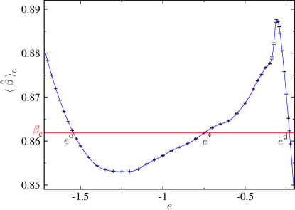
A standard way of studying phase-coexistence in a microcanonical setting is the Maxwell construction. This allows to compute from the curve $\beta(e)$ several important magnitudes: the critical inverse temperature $\beta_{\mathrm{c}}$, the energies of the two coexisting phases and the surface tension. Furthermore, one may apply the very same method to the sample dependent $\langle\hat{\beta}_{\{\epsilon_{i}\}}\rangle_{e}$, as shown in Fig. 2. We follow the numerical methods described in Refs. VICTORMICRO, and POTTS3D, . We briefly summarize them now, for the sake of completeness.

Consider the equation

$$\beta(e)=\beta\,,\quad\text{or (single sample) }\langle\hat{\beta}_{\{\epsilon_{i}\}}\rangle_{e}=\beta\,.$$ (10)

In normal situations, $\beta(e)$ is monotonically decreasing with $e$, so that Eq. (10) has a unique solution. However, at phase-coexistence $\beta(e)$ is no longer monotonically decreasing, see Fig. 2. Therefore, Eq. (10) has three important solutions, named $e^{\mathrm{o}}$, $e^{*}$, and $e^{\mathrm{d}}$ ($e^{\mathrm{o}}<e^{*}<e^{\mathrm{d}}$):

• The rightmost root of (10), $e_{L,\beta}^{\text{d}}$, corresponds to the “disordered phase”.

• The leftmost root of (10), $e_{L,\beta}^{\text{o}}$, corresponds to the “ordered phase”.

• The second rightmost root of (10), $e_{L,\beta}^{*}$ is a saddle-point among the two phases.

Note that these three solutions do depend on $L$, although we shall not explicitly indicate it unless necessary.

We compute the inverse critical temperature $\beta_{\mathrm{c}}$ from the equal-area rule:

$$0=\int_{e^{\text{o}}_{\beta_{\text{c}}}}^{e^{\text{d}}_{\beta_{\text{c}}}}\text{d}e\,\left(\beta(e)-\beta_{\text{c}}\right)\,,$$ (11)

see Fig. 2. Note that the $\beta_{\mathrm{c}}$ computed from Eq. (11) does depend on the system size. In fact, in the thermodynamic limit, Eq. (11) is a mere consequence of the continuity of the free-energy density (as a function of temperature) at the phase transition. In fact, recall that the free energy density can be expressed in terms of the inverse temperature and of the internal energy and entropy densities: $f=e-s/\beta$. Now, if we recall Eq. (7), we see that the equality of the free-energy densities of the ordered and the disordered phases at the critical temperature can be recast as

$$\beta_{\mathrm{c}}(e_{\beta_{\mathrm{c}}}^{\mathrm{d}}-e_{\beta_{\mathrm{c}}}^{\mathrm{o}}) = s(e_{\beta_{\mathrm{c}}}^{\mathrm{d}})-s(e_{\beta_{\mathrm{c}}}^{\mathrm{o}})\,$$ (12)

$$= \int_{e^{\text{o}}_{\beta_{\text{c}}}}^{e^{\text{d}}_{\beta_{\text{c}}}}\text{d}e\,\beta(e)\,.$$ (13)

This textbook reasoning can be extended to the more complicated case of a finite-system. In fact, it is easy to show, see Refs. VICTORMICRO, and JANKEMIC, , that Eq. (11) is identical to the criterion of equal-height in the energy histogram.FSSFO Such a finite-system indicator of the critical temperature suffers from finite-size corrections of order ${\sim 1/L^{D}}$.BORGS-KOTECKY

Once we know $\beta_{c}$, we may compute the latent-heat as

$$\Delta e=e^{\text{d}}_{\beta_{\text{c}}}-e^{\text{o}}_{\beta_{\text{c}}}\,.$$ (14)

Finally, the surface-tension, $\varSigma$, is calculated as

$$\varSigma(L)=\frac{N}{2L^{D-1}}\int_{e^{*}_{\beta_{\text{c}}^{L}}}^{e^{\text{d}}_{\beta_{\text{c}}^{L}}}\mathrm{d}e\,\left(\beta(e)-\beta_{\mathrm{c}}^{L}\right)\,.$$ (15)

Note that, in order to compute integrals such as the one in Eq. (11), we interpolate $\beta(e)$ (which is numerically computed over a grid in the $e$-line), through a cubic spline. Statistical errors are computed using a jackknife method (see e.g. Ref. VICTORMICRO, ). In the case of the sample-averaged $\beta(e)$, the jackknife blocks are formed from the microcanonical mean-values obtained on the different samples. On the other hand, when one performs the Maxwell construction for a single sample as in Fig. 2, the jackknife blocks are formed from the Monte Carlo history.

Figure 3: (Color online) Maxwell construction, see Eq. (11), as obtained for the sample-averaged $\beta(e)$. Data for $L\!=\!48$ and several values of the spin concentration. The transition becomes smoother as $p$ decreases (from bottom to top). In fact, for $p\!=\!0.8$ the Maxwell construction can no longer be done (because the corresponding $\beta(e)$ is monotonically decreasing with $e$).

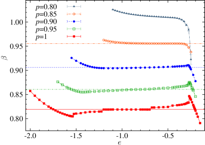
It is interesting to compare the curves $\beta(e)$ for fixed $L\!=\!48$, as the disorder increases (i.e. as $p$ decreases), see Fig. 3. In the limit of a pure system, $p\!=\!1$, $\beta(e)$ displays the expected cusps and steps for a system with well developed geometric and condensation transitions.FOOT_GEOMETRIC As soon as the system becomes disordered, the transition becomes smoother: both the latent heat, see Eq. (14), and the surface tension, Eq. (15), are sizably smaller for $p=0.95$ than for $p=1$. This trend is maintained for decreasing $p$, to the point that the phase transition is clearly of the second order at $p=0.8$ (for that dilution, $\beta(e)$ is monotonically decreasing with $e$). We note as well that the curve $\beta(e)$ for $p<1$ is remarkably featureless, specially if compared to its $p=1$ counterpart. Actually, geometric transitions are also found for individual samples at $p\!=\!0.95$. However, the energies at which this singular behavior arise depend on the considered sample, which results in a smooth averaged $\beta(e)$.

III.3 Finite Size Scaling near a Tricritical Point

In the following we will discuss some relevant facts about the scaling near a tricritical point, see, e.g., Ref.VICTORAMIT, . Consider some quantity $O$, that, in the thermodynamic limit, scales as $O^{(L=\infty)}\sim\xi^{x}$, where $\xi$ is the correlation length. The Finite Size Scaling (FSS) ansatz, tells us how the same quantity behaves in a finite system of size $L$. Close to the tricritical point at $(p_{\mathrm{t}},T_{\mathrm{t}}=T_{\mathrm{c}}(p_{\mathrm{t}}))$

$$O(L,p_{\mathrm{t}}+\delta p,T_{\text{t}}+\delta T)=L^{x}G(L^{y_{T}}u_{T},L^{y_{p}}u_{p})\,,$$ (16)

where $G$ is a scaling function, and we have neglected scaling corrections. As stated in Eqs. (2) and  (3), there are two relevant scaling fields, the thermal field $u_{T}$ and the disorder field $u_{p}$. Both $u_{T}$ and $u_{p}$ are functions of $\delta p$ and $\delta T$, the deviations from the tricritical point. If we work at $u_{T}=0$, we should expect that, at linear order, $\left.u_{p}\right|_{u_{T}=0}\propto\delta p\,$. Then the phase transition is of the second order if $\delta p<0$, and of the first order if $\delta p>0$.

Our main assumption will be that the Maxwell construction, see Ref. VICTORMICRO, and the previous subsection, enforces the constrain $u_{T}=0$ to an accuracy of order ${\cal O}(L^{-D})$ (this expectation is well founded in the first-order part of the critical lineFSSFO ). Hence, Eq. (16) simplifies to

$$O(L,p,\text{Maxwell})=L^{x}\tilde{G}\big{(}L^{y_{p}}(p-p_{\mathrm{t}})\big{)}\big{(}1+{\cal O}(L^{y_{T}-D})\big{)}\,.$$ (17)

So, the Maxwell construction allows us to employ standard FSS,VICTORAMIT with an effective scaling-corrections exponent $\omega=D-y_{T}$. The combination of Eqs. (2) and  (3), standard RFIM scaling relationsNatherman and the numerical estimates in Ref. DAFF-UCM, yield $\omega=\theta+\beta^{\text{RFIM}}/\nu^{\text{RFIM}}=1.48(2)$.

A further irrelevant scaling field $u_{Q}=1/\log Q$ with exponent $-\theta$ is also present.Cardy97 Numerically, $\theta=1.468(2)$ DAFF-UCM , while we expect $\omega=1.48(2)$. These two exponents are so similar that, given our limited numerical accuracy, we shall not attempt to distinguish them. However, we remark that one expects a larger amplitude of the scaling corrections for $Q=4$, what is confirmed by our data (see Fig. 6).

III.4 Numerical Simulations and Thermalization Checks

Figure 4: (Color online) In order to ascertain thermalization, we use the standard logarithmic data binning (data corresponding to $\beta(e)$, as computed for $L=64$, $p=0.95$). Bin 1 was computed from the sample-average of the last half of the Monte Carlo history on each sample (bin 2 corresponds to the second quarter of the Monte Carlo history, bin 3 to the second eighth, and so forth). Statistical compatibility among the different bins is a strong thermalization check. Lines are cubic spline-interpolations for each bin. In order to demonstrate the importance of having a dense enough simulation grid (in particular, close to high curvature regions), the spline interpolation in the blue line ignores the data at $e=-0.2875$.

$L$	Simulated $p$ values
12	0.65, 0.675, 0.7, 0.725, 0.75, 0.775, 0.8, 0.825, 0.832, 0.85, 0.875, 0.9, 0.925, 0.9375, 0.95
16	0.65, 0.675, 0.7, 0.725, 0.75, 0.775, 0.8, 0.825, 0.85, 0.854, 0.875, 0.9, 0.925, 0.9375, 0.95
24	0.7, 0.725, 0.75, 0.775, 0.8, 0.825, 0.832, 0.845, 0.85, 0.875, 0.9, 0.925.
32	0.75, 0.775, 0.8, 0.825, 0.85, 0.854, 0.8625, 0.875, 0.886, 0.8875, 0.9, 0.925, 0.9375, 0.95, 0.975.
48	0.75, 0.775, 0.8, 0.825, 0.85, 0.8625, 0.875, 0.877, 0.8875, 0.9, 0.925, 0.9375, 0.95.
64	0.8, 0.825, 0.85, 0.86875, 0.875, 0.8875, 0.9, 0.925, 0.9375, 0.95.

Table 1: For each of the lattice sizes $L$, we indicate the values of $p$ (the concentration of magnetic sites) for which we carried out simulations. We shall need to regard the various quantities defined, as continuous functions of the density of magnetic sites, $p$. We shall need as well the corresponding $p$-derivatives. As a rule, we have obtained these functions of $p$ through a cubic-spline interpolation of the data computed at these $p$-values. In fact, some of them were chosen in order to minimize the interpolation errors at some particularly important values of $p$, see Tables 2 and 3. Derivatives with respect to $p$ were computed simply by derivating the cubic-spline interpolating function. The error estimates where obtained through a jack-knife (see for instance Ref. VICTORAMIT, ) over the sample-averages.

We considered concentration values $0.65\leq p\leq 1$ and lattice sizes $12\leq L\leq 64$. The precise values are indicated in Table 1. The $p$-resolution becomes denser close to the $L$-dependent position of the tricritical point. For all pairs ($p$, $L$) we simulated 500 samples, with the obvious exception of $p\!=\!1$.

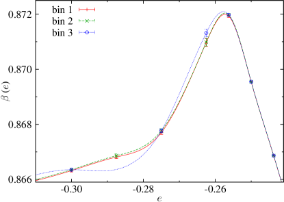
Each sample was simulated on a $e$-grid fine enough to allow for a correct spline interpolation, see Fig. 4. The simulations at the different $e$ values were mutually independent. Hence, we faced an embarrassingly parallel computational problem, suitable for Ibercivis (with a caveat, see below).

All samples were simulated for the same number of Monte Carlo steps, at every $e$ value. However, the number of Monte Carlo steps did depend on $e$, as we explain now. First, we ran all samples at a given $e$-value for a fixed amount of Swendsen-Wang steps (e.g. $3\times 10^{5}$ for $L\!=\!64$, or $2\times 10^{5}$ for $L\!=\!48$), then we assessed thermalization.

The thermalization check was the standard logarithmic data-binning: for any given value of $e$, we computed different estimates of the sample-averaged $\beta(e)$, using disjoint pieces of the Monte Carlo history. On the first bin, we included only the second-half of the Monte Carlo history (i.e., our safest data from the point of view of thermalization). The second bin contained only the second quarter of the Monte Carlo history, etc. We checked for statistical compatibility, at least, among the first and second bins, see Fig. 4. If for a given value of $e$ the thermalization criterion was not met, the total simulation time was doubled. The procedure was cycled until convergence was achieved. We note that, for the concentrations nearest to $p=1$, we encountered strong metastabilities, that prevented us from simulating $L\!=\!128$ (that could instead be simulated for $Q\!=\!4$ in Ref. POTTS3D, ).

The thermalization protocol is not well suited for Ibercivis, because the simulation of a given sample at some difficult energy may last up to some days. Yet, Ibercivis relies on volunteers’ computers that frequently switch from on-line to off-line. To minimize the number of unfinished simulations, we have implemented a continuity system. It divides every simulation, no matter how long it is, in small time steps (typically 30 minutes). After every step, consistency checks are performed and the current system configuration is sent again to the simulation queue. This solved the problem for relatively long (5-6 hours) simulations but the few more demanding simulations were completed on local clusters.

Altogether, this work has consumed (the equivalent of) $3\times 10^{6}$ hours of a single Intel Core2 duo at 2.5 GHz.

We should also mention that we have performed some new, short simulations for $Q=4$ at $p=0.95$, complementary to those reported in Ref. POTTS3D, . The simulated sizes were $L=24$ and $L=48$ (128 samples each). Our goal was to improve the accuracy of the interpolations described below.

IV Results

To check the Cardy-Jacobsen conjecture we have performed numerical simulations for $Q=8$, hence further approaching the large-$Q$ limit where the mapping becomes exact.Cardy97

Figure 5: (Color online) Latent heat $\Delta e$ (Top) and surface tension $\varSigma$ (Middle) as a function spin concentration, $p$, for each lattice size (lines are linear interpolations). Lines end at the smallest $p$ that allowed to perform the Maxwell construction for each $L$. Bottom: Scaled surface tension using $\theta=1.469(20)$ DAFF-UCM (the lines joining the data are cubic splines). The vertical gray line shows the infinite volume extrapolation for $p_{\mathrm{t}}$.

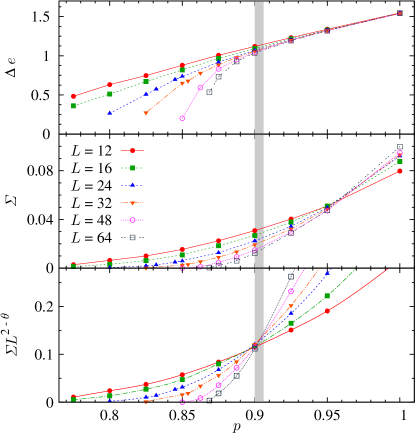
Consider the $p$ and $L$ evolution of the latent-heat and the surface tension in Fig. 5. If $p\!<\!p_{\text{t}}$ (i.e. if we are in the second-order piece of the critical line), both $\Delta e$ and $\varSigma$ vanish in the large-$L$ limit (the two are positive for $p\!>\!p_{\text{t}}$). However, for small lattices, both $\Delta e$ and $\varSigma$ decrease gently upon decreasing $p$ which suggests that dilution merely smoothed the first-order transition. However, the curve for $\Delta e$ becomes sharper upon increasing $L$. Indeed the Potts-RFIM mappingCardy97 implies $\Delta e\propto(p-p_{\text{t}})^{\beta}$ with $\beta\!=\!\beta^{\mathrm{RFIM}}\!\sim\!0.01$,Natherman which is barely distinguishable from a discontinuous jump. Furthermore, the $L$-dependent position of the tricritical point $p_{\mathrm{t}}^{L}$ (for instance, the point of sharpest drop of $\Delta e$ in Fig. 5—top) grows quickly with $L$. On the view of the $D\!=\!2$ no-go theorems,Aize89 one could be afraid that $p_{\mathrm{t}}^{L}\to 1$ for large $L$ also in $D\!=\!3$. We know that this is not the case,POTTS3D but it is clear that a careful scaling analysis is needed.

Eq. (17) tells us that $L^{2-\theta}\varSigma$ is scale-invariant, and thus allows to locate the tricritical point (because $x_{\varSigma}\!=\!\theta-D+1\!=\!\theta-2$, $\theta\!=\!1.469(20)$ DAFF-UCM ). Indeed, in Fig. 5—bottom, we see that the curves for system sizes $L_{1}<L_{2}$ cross at $p_{\mathrm{t}}^{L_{1},L_{2}}$:

$$L_{1}^{2-\theta}\varSigma(L_{1},p_{\mathrm{t}}^{L_{1},L_{2}})=L_{2}^{2-\theta}\varSigma(L_{2},p_{\mathrm{t}}^{L_{1},L_{2}})\,,$$ (18)

($p_{\text{t}}^{L_{1},L_{2}}\to p_{\mathrm{t}}$ when $L_{1}$ diverges). We recall that a similar method was used recently in a spin-glass context.Janus2010corto There are two main consequences of choosing a wrong estimate of exponent $\theta$ in Fig. 5—bottom and Eq. (18). First, in the limit of large lattice sizes, the height of the crossing point diverges (or goes to zero) if $\theta$ is underestimated (overestimated). Second, the size corrections to the crossing points are larger for a wrong $\theta$. Specifically, $p_{\mathrm{t}}^{L_{1},L_{2}}-p_{\text{t}}\!=\!{\cal O}(L_{1}^{-y_{p}})$. The amplitude for these scaling corrections cancels only for the exact choice of $\theta$.

The critical exponent for a quantity $O$ is obtained from its quotients at $p_{\mathrm{t}}^{L_{1},L_{2}}$:QUOTIENTS ; NIGHTINGALE

$$\left.\frac{O(L_{2})}{O(L_{1})}\right|_{p_{\mathrm{t}}^{L_{1},L_{2}}}=\left(\frac{L_{2}}{L_{1}}\right)^{x_{O}}\,\left[1+A_{O}\bigg{(}\frac{1}{L_{2}^{\omega}}-\frac{1}{L_{1}^{\omega}}\bigg{)}\right]\,.$$ (19)

Above, we included only the leading scaling-corrections ($A_{O}$ is an amplitude). We use Eq. (19) for the logarithmic $p$-derivative of $\varSigma$ (scaling dimension $x=y_{p}$), and for the latent heat (scaling dimension $x=\beta y_{p}$, which should be $\beta^{\text{RFIM}}/\nu^{\text{RFIM}}$, according to Cardy and JacobsenCardy97 ). Our results are in Table 2 ($Q=8$), and Table 3 ($Q=4$). In both cases we see that the convergence of $p_{t}^{L_{1},L_{2}}$ to the thermodynamic limit is very fast. The height of the crossing point seems also stable with growing sizes.

$(L_{1},L_{2})$	$p_{t}^{L_{1},L_{2}}$	$y_{p}$	$L_{1}^{2-\theta}\varSigma^{\text{cross}}$	$\beta y_{p}$
(12,16)	0.8947(38)(17)	0.89(23)(2)	0.108(5)(3)	0.095(9)(5)
(12,24)	0.8942(16)(15)	0.82(8)(2)	0.107(3)(3)	0.075(3)(4)
(16,24)	0.8939(28)(14)	0.79(18)(3)	0.107(6)(4)	0.061(5)(3)
(16,32)	0.8966(13)(11)	0.85(13)(3)	0.111(3)(4)	0.050(2)(2)
(24,32)	0.8989(28)(10)	0.94(26)(3)	0.118(8)(5)	0.035(5)(2)
(24,48)	0.9031(14)(10)	0.80(6)(05)	0.128(4)(6)	0.027(2)(2)
(32,48)	0.9057(21)(9)	0.84(10)(1)	0.139(8)(7)	0.021(4)(2)
(32,64)	0.9040(11)(8)	0.86(5)(1)	0.134(5)(7)	0.023(3)(1)
(48,64)	0.9026(21)(5)	0.99(14)(3)	0.126(10)(8)	0.024(6)(1)

Table 2: Quotient-method for $Q=8$. For each pair of lattices $(L_{1},L_{2})$, we extract the crossing point $p_{t}^{L_{!},L_{2}}$, see Eq. (18), and the height of the crossing point, $\varSigma(L_{1},p_{t}^{L_{1},L_{2}})L_{1}^{2-\theta}$. The effective critical exponents $y_{p}$ and $\beta y_{p}$ are obtained using the quotients method, Eq. (19). For each data, we indicate two error bars. The first error is statistical. The second error is due to the uncertainty in $\theta=1.469(20)$.DAFF-UCM

$(L_{1},L_{2})$	$p_{\mathrm{t}}^{L_{1},L_{2}}$	$y_{p}$	$L_{1}^{2-\theta}\varSigma^{\text{cross}}$	$\beta y_{p}$
(16,24)	0.9249(30)(8)	1.40(46)(3)	0.0113(6)(5)	0.285(11)(6)
(16,32)	0.9324(19)(8)	1.11(20)(5)	0.0125(5)(6)	0.230(6)(6)
(24,32)	0.9400(30)(6)	1.22(33)(1)	0.0159(12)(8)	0.175(12)(4)
(24,48)	0.9455(19)(9)	0.83(8)(3)	0.0179(9)(8)	0.135(5)(4)
(32,48)	0.9506(27)(8)	0.79(18)(3)	0.0215(17)(10)	0.112(7)(3)
(32,64)	0.9489(13)(7)	0.78(9)(2)	0.0206(9)(11)	0.095(4)(3)
(48,64)	0.9473(31)(5)	0.92(24)(3)	0.0191(25)(12)	0.070(10)(3)
(48,128)	0.9491(9)(5)	0.77(8)(2)	0.0204(10)(13)	0.048(4)(3)
(64,128)	0.9497(14)(5)	0.71(13)(2)	0.0213(17)(14)	0.038(6)(3)

Table 3: Quotient method for $Q=4$ (data from Ref. POTTS3D, , improved through control variates and the addition of new runs near $p_{\mathrm{t}}$). Same notations of Table 2.

The results in Tables 2 and 3 need to be extrapolated to the limit of infinite system sizes. This can be done by considering leading order scaling corrections, as in Eq. (19). The extrapolation greatly improves by imposing to $Q=4$ and $8$ a common extrapolation and the same scaling-corrections exponent $\omega$, as required by the Universality predicted in Ref. Cardy97, .

In this way, we obtain $\beta y_{p}=0.0022(48)(3)$ and $\omega=1.36(8)(1)$ where the second parenthesis indicates the uncertainty induced by the error in $\theta$.DAFF-UCM The fit quality is assessed through the $\chi^{2}$ test. We obtain $\chi^{2}/\mathrm{dof}=8.5/14$, which is almost too good (dof stands for the number of degrees of freedom of the fit). Indeed the probability of getting such a low value of $\chi^{2}$ with 14 degrees of freedom is only $14\%$. We note as well that $\beta y_{p}=0.0022(48)(3)$ is only barely compatible with the best RFIM estimate $\beta y_{p}=0.0119(4)$,DAFF-UCM (since the discrepancy is as large as two standard deviations).

At this point, we can try to disproof universality. We make the assumption that $\beta y_{p}$ takes exactly the RFIM value, redo the fit and see the outcome of the $\chi^{2}$ test. This second fit, with $\beta y_{p}$ fixed to $0.0119$, turns out to be perfectly reasonable ($\chi^{2}/\text{dof}=14/15$, see Fig. 6). Hence we conclude that our data set is statistically compatible with universality.

A second, unexpected bonus of fixing $\beta y_{p}$ in the fit to the RFIM value, is a remarkable increase in the accuracy of $\omega=1.53(5)(3)$, in excellent agreement with our expected $\omega=1.48(2)$ (remember that $\omega=D-y_{T}=\theta+\beta^{\text{RFIM}}/\nu^{\text{RFIM}}$, see Sec. III.3). Furthermore, from this value of $\omega$, we obtain $y_{T}=D-\omega=1.47(8)$, in nice agreement with the large-$Q$ computation $y_{T}=1.49(9)$.Igloi2006

Figure 6: (Color online) Determination of the scaling correction exponent $\omega$, from the size-dependent effective exponent $\beta y_{p}$ for the vanishing latent-heat at the tricritical point as computed with the quotients method, see Tables  2 and 3. A common extrapolation $\beta y_{p}\!=\!0.0119(4)$ DAFF-UCM is imposed in the joint-fit for the $Q\!=\!4$ and $Q\!=\!8$ data. The figure of merit $\chi^{2}=14/15$ is computed with the full covariance matrix.

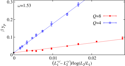
Following the same approach for $y_{p}$, which is expected to coincide with $1/\nu^{\text{RFIM}}$, we obtain $y_{p}=0.775(46)(1)$ if we impose $\omega=1.36$ (we get $y_{p}=0.779(41)(1)$ by taking $\omega=1.53$). Both fits are fair ($\chi^{2}/\text{dof}=13.6/15$ and $\chi^{2}/\text{dof}=13.2/15$, respectively).

Our $y_{p}$ is in the lower range of previous numerical and analytical estimates: $0.73\leq 1/\nu^{\text{RFIM}}\leq 1.12$.DAFF-UCM ; Ogielski86 ; Gofman ; Newman96 ; Swift97 ; Rieger95 ; Dukovski03 ; Angles97 ; Nowak98 ; Nowak99 ; Middleton02 ; Hartmann ; NPFRG Hyperscaling and our $y_{p}$ implies a slightly positive specific heat exponent $\alpha=(2y_{p}-D+\theta)/y_{p}=0.03(10)$, in agreement with experimental claims of a (possibly logarithmic) divergence.EXPO-ALPHA-BELANGER We warn however that severe hyperscaling violations [namely $\alpha=-0.63(7)$] have been reported in numerical work.Hartmann

One may compute as well the exponent $\theta$, by fitting $\varSigma(L,p_{\text{t}}^{L,2L})=A_{Q}L^{\theta}(1+B_{Q}L^{-\omega})$ (only the amplitudes $A_{Q}$ and $B_{Q}$ are $Q$-dependent on the fit). Taking $\omega=1.5(1)$, we obtain $\theta=1.52(11)(2)$, with an acceptable fit ($\chi^{2}/\mathrm{dof}=4.9/3$). The result is compatible with, but less accurate than, the latest RFIM result $\theta=1.469(20)$.DAFF-UCM

V Conclusions

In summary, we have presented a finite-size scaling analysis of the tricritical point of the site-diluted Potts model in three dimensions for $Q=4$ and $8$ internal states. By considering leading-order scaling corrections we were able to show that the relevant Universality class for the tricritical point is the one of the RFIM. To our knowledge, this is the first verification of the Cardy-Jacobsen conjecture.Cardy97

Three technical ingredients were crucial to obtain this achievement: the use of the microcanonical Monte Carlo,VICTORMICRO a new definition of the disorder average,POTTS3D and the use of the citizen supercomputer Ibercivis.IBERCIVIS1

VI Acknowledgements

We have been partly supported through Research Contracts Nos. FIS2009-12648-C03 and FIS2010-16587 (MICINN), GR10158 (Junta de Extremadura), ACCVII-08 (UEX), and from UCM-Banco de Santander. We thank Ibercivis for the equivalent of $3\times 10^{6}$ CPU hours. The simulations were completed in the clusters Terminus (BIFI) and Horus (U. Extremadura). We also thank N. G. Fytas for a careful reading of the manuscript.

Appendix A Control variates

The statistical quality of data may sometimes be significantly increased by means of a very simple trick, named control variates (see e.g. Ref. CV-UCM, ).

Figure 7: (Color online) Scatter plot of each sample’s inverse critical temperature vs. the concentration of magnetic sites, $\sum_{i}\epsilon_{i}/V$. Data for 500 samples of $L=64$ and $p=0.95$. The correlation coefficient that gives the optimal coupling to the control variate, see Eq. (20), is $\alpha^{*}=0.956$.

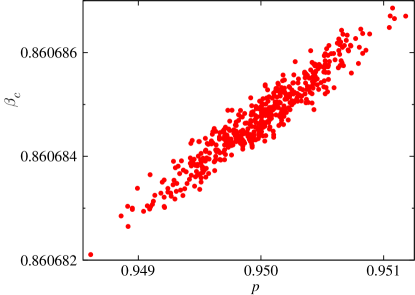
In short, we want to improve our estimation of a stochastic variable $A$ through its correlations with another random variable $B$ ($B$ is named a control variate). If $\overline{B}=0$ and $\hat{A}=A+\alpha B$, then the expectation value does not change: $\overline{\hat{A}}=\overline{A}$. However, depending on the arbitrary election of $\alpha$, we can get $\text{var}(\hat{A})<\text{var}(A)$. The $\alpha$ election minimizing the variance $\text{var}(\hat{A})$ is

$$\alpha^{*}=\frac{\text{cov}(A,B)}{\sqrt{\text{var}(A)\text{var}(B)}}\,,$$ (20)

which coincides with the correlation coefficient $r_{AB}$. The optimal variance is

$$\text{var}(\hat{A}^{*})=\text{var}(A)\,(1-r^{2}_{AB})\,.$$ (21)

Hence, the stronger the statistical correlation (or anticorrelation) between $A$ and $B$, the more effective the control variate is.

Figure 8: (Color online) Inverse critical temperature $\beta_{\mathrm{c},L}$ as a function of an inverse lattice volume, $1/L^{3}$. Data obtained for $p=0.95$. The error reduction obtained with control variates is significant (blue points). In the linear fit we considered only data with $L\geq 16$ and improved through control variates.

Figure 9: (Color online) The size dependent latent-heat for $p=0.95$, as a function of the inverse lattice volume. The linear fit includes only data with $L\geq 16$ that were improved through control variates.

In our case, a rather obvious control variate is

$$B=\frac{1}{V}\sum_{i}\epsilon_{i}\ -\ p\,,$$ (22)

namely the difference among the real and the nominal concentrations of magnetic sites. It is clear that the disorder average $\overline{B}$ vanishes. We will employ $B$ to improve the determination of the sample-averaged $\beta(e)$. Note that, although the value of $B$ does not depend on the considered energy (it is fixed by the $\{\epsilon_{i}\}$), its correlation coefficient with $\langle\hat{\beta}\rangle_{e}$ needs to be computed for all energies in the $e$-grid.

$B$ is extremely effective as a control variate for the computation of the inverse critical temperature $\beta_{\mathrm{c}}$, as suggested from Fig. 7. The correlation coefficient in that plot is so high, 0.956, that the expected error reduction factor is 3.4. However, the alert reader will note that this is a hasty conclusion. In fact, the $\beta_{\text{c}}$ obtained from $\beta(e)$ is not exactly the average of the inverse critical temperatures found for each sample. The reason for this non-linearity in the Maxwell rule, see Eq. (11), is that the energies $e^{\mathrm{d,o}}$ are not the same for $\beta(e)$ and for the $\langle\hat{\beta}\rangle_{e}$ in a given sample. Yet, the dependency on $e^{\mathrm{d,o}}$ of the integral in Eq. (11) is extremely weak [recall the stationarity condition with respect to $e$ in Eq. (10)].

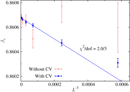
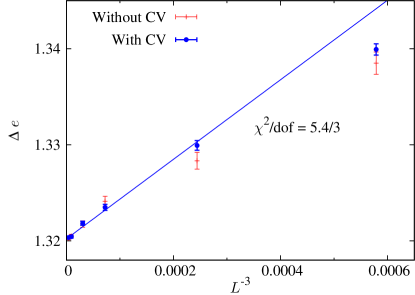
In fact, the correct computation with $\beta(e)$ does show a significant error reduction, see Fig. 8, close to the factor 3.4 anticipated by the naive analysis in Fig. 7. We note in Fig. 9 an equally significant reduction of the statistical errors for the latent heat. Therefore, our computation of these quantities, obtained with only 500 samples, has been made equivalent to a 5000-samples computation. This is a remarkable reward for such a simple analysis.

References

- (1) E. Dagotto, Science 309, 258 (2005); J. Burgy, M. Mayr, V. Martin-Mayor, A. Moreo and E. Dagotto, Phys. Rev. Lett. 87, 277202 (2001); J. Burgy, A. Moreo, and E. Dagotto, ibid 92, 097202 (2004); C. Sen, G. Alvarez and E. Dagotto, Phys. Rev. Lett. 98, 127202 (2007).
- (2) See e.g. G. Parisi Field Theory, Disorder and Simulations. World Scientific 1994.
- (3) G. Xu, W. Jiang, M. Qian, XX. Chen, ZB. Li and GR. Han, Crystal Growth & Desing 9, 13 (2009).
- (4) H. Koibuchi, Phys. Rev. E 77, 021104 (2008).
- (5) ZN. Hu and VC. Lo, Commun. Theor. Phys. 48, 183 (2007).
- (6) JF. Scott et al, J. Am. Ceram. Soc. 88 1691 (2005).
- (7) H. Westfahl and J. Schmalian, Phys. Rev. E 72, 011806 (2005).
- (8) II. Naumov, L. Bellaiche and HX. Fu Nature 432, 737 (2004).
- (9) M. Freedman, C. Nayak, K. Shtengel, K. Walker and ZH. Wang, Ann. Phys. 310, 428 (2004).
- (10) R. Berthet, A. Petrossian, S. Residori, B. Roman and S. Fauve, Physica D 174, 84 (2003).
- (11) S. Residori, R. Berthet, B. Roman and S. Fauve, Phys. Rev. Lett. 88, 024502 (2001).
- (12) M. Aizenman and J. Wehr, Phys. Rev. Lett. 62, 2503 (1989); K. Hui and A.N. Berker ibid 62, 2507 (1989).
- (13) J. Cardy and J. L. Jacobsen, Phys. Rev. Lett. 79, 4063 (1997); J. L. Jacobsen and J. Cardy, Nucl. Phys. B 515, 701 (1998); J. Cardy, at STATPHYS20 conference, North-Holland (1999), arXiv:9806355.
- (14) C. Chatelain and B. Berche, Phys. Rev. Lett. 80, 1670 (1998); Phys. Rev E 58, R6899 (1998); ibid 60, 3853 (1999).
- (15) T. Natherman: In Spin glasses and random fields, edited by A. P. Young (World Scientific, Singapore, 1998).
- (16) D. P. Belanger: In Spin glasses and random fields, edited by A. P. Young (World Scientific, Singapore, 1998).
- (17) F.Y. Wu, Rev. Mod. Phys. 54, 235 (1982).
- (18) J. Bricmont, A. Kupiainen, Phys. Rev. Lett. 59, 1829 (1987).
- (19) L. A. Fernandez, A. Gordillo-Guerrero, V. Martin-Mayor, and J. J. Ruiz-Lorenzo, Phys. Rev. Lett. 100, 057201 (2008).
- (20) M. T. Mercaldo, J-Ch. Angles d’Auriac and F. Igloi, Phys. Rev. E 73, 026126 (2006).
- (21) One may fit spin-glass interactions into the same scheme, see Ref. Paoluzzi10, ; Leuzzi11, .
- (22) Z. Slanic, D. P. Belanger and J. A. Fernandez-Baca, Phys. Rev. Lett. 82, 426 (1999).
- (23) F. Ye et al. Phys. Rev. Lett. 89, 157202 (2002).
- (24) L. A. Fernandez, V. Martin-Mayor, and D. Yllanes, Phys. Rev. B 84, 100408(R) (2011).
- (25) A. T. Ogielski, Phys. Rev. Lett. 57, 1251 (1986).
- (26) M. Gofman, J. Adler, A. Aharony, A. B. Harris and M. Schwartz, Phys. Rev. Lett. 71, 1569 (1993).
- (27) M. E. J. Newman and G. T. Barkema, Phys. Rev. E 53, 393 (1996).
- (28) M. R. Swift, A. J. Bray, A. Maritan, M. Cieplak and J. R. Banavar, Europhys. Lett. 38, 273 (1997).
- (29) H. Rieger, Phys. Rev. B 52, 6659 (1995).
- (30) I. Dukovski and J. Machta, Phys. Rev. B 67, 014413 (2003).
- (31) J.-C. Angles d’Auriac and N. Sourlas, Europhys. Lett. 39, 473 (1997).
- (32) U. Nowak, K. D. Usadel, and J. Esser, Physica A 250, 1 (1998)
- (33) A. K. Hartmann and U. Nowak, Eur. Phys. J. B 7, 105(1999)
- (34) A. A. Middleton and D. S. Fisher, Phys. Rev. B 65, 134411 (2002).
- (35) A. K. Hartmann and A. P. Young, Phys. Rev. B 64, 214419 (2001).
- (36) N. Sourlas, Comp. Phys. Comm. 121, 183 (1999).
- (37) A. Maiorano, V. Martin-Mayor, J. J. Ruiz-Lorenzo, and A. Tarancón, Phys. Rev. B 76, 064435 (2007).
- (38) H. G. Ballesteros, L. A. Fernández, V. Martin-Mayor, A. Muñoz Sudupe, G. Parisi and J. J. Ruiz-Lorenzo. Phys. Rev. B 61, 3215 (2000).
- (39) C. Chatelain, B. Berche, W. Janke, and P.-E. Berche, Phys. Rev. E 64, 036120 (2001).
- (40) C. Chatelain, B. Berche, W. Janke, and P.-E. Berche, Nucl. Phys. B 719, 275 (2005).
- (41) M. Paoluzzi, L. Leuzzi, and A. Crisanti, Phys. Rev. Lett. 104, 120602 (2010).
- (42) L. Leuzzi, M. Paoluzzi, and A. Crisanti, Phys. Rev. B 83, 014107 (2011).
- (43) A. Malakis, A. Nihat Berker, N. G. Fytas, T. Papakonstantinou, arXiv:1203.0985.
- (44) V. Martin-Mayor, Phys. Rev. Lett. 98, 137207 (2007).
- (45) Ibercivis (http://www.ibercivis.net) provides nowadays as much as computing cores (this quantity fluctuates, depending on the number of volunteers on line). The current count of volunteers is and growing.
- (46) D. Amit and V. Martin-Mayor, Field Theory, the Renormalization Group and Critical Phenomena, (World-Scientific Singapore, third edition, 2005).
- (47) Remember that the parameter that plays the role of the reduced temperature in the RFIM is ,Natherman . In the Cardy-Jacobsen mapping, the disorder strength in the Potts model, , corresponds exactly with .Cardy97 Hence, . However, keep in mind that this relation was obtained by reasoning in the limit .
- (48) L. A. Fernandez, A. Gordillo-Guerrero, V. Martin-Mayor, and J. J. Ruiz-Lorenzo, Phys. Rev. E 80, 051105 (2009).
- (49) W. Janke, Nucl. Phys. B (Proc. Suppl.) 63, 631 (1998).
- (50) M. S. S. Challa, D. P. Landau, and K. Binder, Phys. Rev. B 34, 1841 (1986); J. Lee and J. M. Kosterlitz, Phys. Rev. Lett. 65, 137 (1990).
- (51) C. Borgs and R. Kotecký, Phys. Rev. Lett. 68, 1734 (1992).
- (52) In a system with periodic boundary conditions, geometrical transitions arise when the energy varies from the ordered to the disordered phase. In fact, the system struggles to minimize the surface energy while respecting the global constraint for . Depending on the fraction of ordered phase, which is fixed by , the minimizing geometry can be either a bubble, a cylinder or a slab of ordered phase in a disordered matrix (or vice versa). As varies, the minimizing geometry changes at definite values. This phenomenon is named geometric transition,GEOMETRIC and it is the reason underlying the steps and the flat central region for , shown in Fig. 3. On the other hand, the two cusps (one lies near to while the other is close to ) are sometimes named size-dependent spinodal points. They are due to the condensation transition.CONDENSATION
- (53) R. A. Baños et al. (Janus Collaboration), Phys. Rev. Lett. 105, (2010) 177202.
- (54) H. G. Ballesteros, L. A. Fernandez, V. Martin-Mayor, A. Muñoz Sudupe, Phys. Lett. B 378, 207 (1996); B 387, 125 (1996); Nucl. Phys. B 483, (1997) 707.
- (55) M. P. Nightingale, Physica A 83, 561 (1976).
- (56) M. Tissier and G. Tarjus, Phys. Rev. B 85, 104203 (2012).
- (57) D. P. Belanger, A. R. King, V. Jaccarino, and J. L. Cardy, Phys. Rev. B 28, 2522 (1983); D. P. Belanger and Z. Slanic, J. Magn. and Magn. Mat. 186, 65 (1998).
- (58) L. A. Fernandez, and V. Martin-Mayor, Phys. Rev. E 79, 051109 (2009).
- (59) K. T. Leung and R. K. P. Zia, J. Phys. A 23, 4593 (1990); L. G. MacDowell, V. K. Shen, and J. R. Errington, J. Chem. Phys. 125, 034705 (2006).
- (60) M. Biskup, L. Chayes, and R. Kotecký, Europhys. Lett. 60, 21 (2002); K. Binder, Physica A 319, 99 (2003); L. G. MacDowell, P. Virnau, M. Müller, and K. Binder, J. Chem. Phys. 120, 5293 (2004); A. Nußbaumer, E. Bittner, T. Neuhaus, and W. Janke, Europhys. Lett. 75, 716 (2006).