Luttinger liquid theory of purple bronze $Li_{0.9}Mo_{6}O_{17}$ in the charge regime.

Abstract

Molybdenum purple bronze Li_0.9Mo₆O₁₇ is an exceptional material known to exhibit one dimensional (1D) properties for energies down to a few meV. This fact seems to be well established both in experiments and in band structure theory. We use the unusual, very 1-dimensional band dispersion obtained in ab-initio DFT-LMTO band calculations as our starting point to study the physics emerging below 300meV. A dispersion perpendicular to the main dispersive direction is obtained and investigated in detail. Based on this, we derive an effective low energy theory within the Tomonaga Luttinger liquid (TLL) framework. We estimate the strength of the possible interactions and from this deduce the values of the TLL parameters for charge modes. Finally we investigate possible instabilities of TLL by deriving renormalization group (RG) equations which allow us to predict the size of potential gaps in the spectrum. While $2k_{F}$ instabilities strongly suppress each other, the $4k_{F}$ instabilities cooperate, which paves the way for a possible CDW at the lowest energies. The aim of this work is to understand the experimental findings, in particular the ones which are certainly lying within the 1D regime. We discuss the validity of our 1D approach and further perspectives for the lower energy phases.

I Introduction.

The molybdenum purple bronze, $Li_{0.9}Mo_{6}O_{17}$ , is a subject of intensive experimental studies already for more than two decadesMcCarroll-first , but its unusual properties remain unclear. Several very different experimental probes have been used: angle resolved photo-emission (ARPES)JWAllen-old , scanning tunnelling microscopy (STM)Hager-bron-STM , DCGreenblatt-old-res-anis and magneto- resistivityHussey-rhoB , thermal conductivity Hussey-thermo , optical conductivityMandrus-optics , Nernst signalSantos-Nernst-2D , muons spectroscopyChakhalian-muons , X-raysOnoda-structure-Xray , thermal expansionSantos-thermal-expan , neutron scatteringSantos-structure-neutrons . Although the main effort of those investigations was focused on the nature of a mysterious phase transition at around 25K, interesting knowledge about higher energy phase was also gathered. Certain properties of the one dimensional (1D) metal, the Luttinger liquid (TLL), have been invoked to explain the measured dataJWAllen-old ; Hager-bron-STM ; JWAllen-1D+2D ; JWAllen-comment-Greenblatt and nowadays the presence of the 1D physics is well established experimentallyJWAllen-high-bulk ; JWAllen-growth-meth , at least in some energy range.

On the theoretical side, band structure calculations have shown a quasi-1D character of molybdenum purple bronze. A remarkably simple band structure emerges from rather complex crystal structure. At the Fermi surface there are only two bands, lying very close to each other, in the form of flat sheets dispersing well only along the b-axis. This gives a hope that purple bronze can indeed be a rare realization of the 1D physics.

The key problem is that several possible mechanisms has been invoked to explain the observed properties, which made the subject quite unclear and controversial. In our opinion the reason for this situation is that each of previous attempts was focused only on one out of many peculiar properties of $Li_{0.9}Mo_{6}O_{17}$ and most of them searched for an explanation in the low energy regime (below $5meV$), where indeed the properties of $Li_{0.9}Mo_{6}O_{17}$ are the most spectacular. By now, not enough attention has been paid even to the parameters of the 1D state. It is only agreed that it emerges at energies as high as 250meV. The values of these parameters are the first issue one must determine before pursuing research towards low energy regimes. The unusual physics observed in $Li_{0.9}Mo_{6}O_{17}$ at the energy scales of order 10meV is obviously a motivation for revising the question of the 1D physics. In order to establish a proper low energy effective theory one has to begin at highest energies and the step by step move towards the physics taking place around Fermi energy. The first step is to link the results of the DFT calculations with the well defined field theory describing the experimental results at around 20meV. It is this ”high energy” regime which must be well understood first. This is the main task of this paper.

The plan of this work is as follows. In Sec.II we begin with a brief introduction of the band structure. In the following section Sec.III.1 we propose a tight binding model which is able to approximate bands around the Fermi energy $E_{F}$, however in addition it contains also the strong correlation terms, beyond the LDA-DFT. In Sec.III.2 we give basic notions of 1D physics, used in the rest of the paper. Section Sec.IV is dedicated to intra-chain physics: we give values parameterizing strong correlations (Sec.IV.1), estimate TLL parameters which this implies (Sec.IV.2) and give energy scales for the spin sector (Sec.IV.4). In section Sec.V we introduce the inter-chain physics. Once again, first we estimate the strength of these interactions (Sec.V.1) and then (Sec.V.2) cast as many of them as possible into effective LL description, now within the ladder framework. Later in Sec.VI we study how the non-linear interaction terms will affect the Luttinger liquid parameters and what instabilities they can potentially produce. Finally in Sec.VII we discuss our results for LL parameters in a context of the experimental findings (Sec.VII.1), as well as the validity of the 1D approach itself in Sec.VII.2. We also discuss in Sec.VIII the role of substitutional disorder in our model. The conclusions in Sec.IX close the paper.

II Band structure

The lattice space group and atomic positions within the structure are known from experiment done by Onoda et al Onoda-structure-Xray recently confirmed by the neutron diffraction experimentSantos-structure-neutrons . This rather complicated structure, which consist of well separated slabs parallel to b-c plane, is presented on Fig.1a). Based on this crystallography knowledge the electronic structure of Li₂Mo₁₂O₃₄ can be calculated using density functional theory (DFT) e.g. in the local density approximation (LDA). Recent calculations Thomas lead to results which are globally consistent with several previous computationsPopovic-bron-DFT ; Canadell-DFT-old . Overall the band dispersions agree well with the measured results obtained by angle resolved photoemission spectroscopy (ARPES) JWAllen-alphaRG . For example it shows a flattening of the two dispersive bands at about 0.4-0.5 eV below $E_{F}$. Other bands are found at least 0.25 eV below $E_{F}$. The only visible discrepancies are the relative vertical shifts of the bands of order 0.1eV. The computed ratio between the Fermi velocities along b- and c-crystal axis, is about 40, compatible with the reported anisotropic 1D-like resistivity Greenblatt-old-res-anis ; Mandrus-optics ; Santos-transport-weird ; Hussey-rhoB . The velocity along $\vec{a}$ is even smaller. At low energies (around Fermi energy $E_{F}$) all calculations gave qualitatively similar results. There are only two bands which cross the Fermi energy and they are placed very close to each other. They have a strong dispersion in the $\Gamma-Y$ direction (b-axis) and barely no dispersion in the perpendicular directions.

The two bands originate from a pair of zig-zag chains build out of $Mo$ atoms inside $O$ octahedra. The low energies (close to $E_{F}$) spectral function is located mostly on $4d$ (precisely $t_{2g}$) orbitals of $Mo(1)$ and $Mo(4)$ atoms, using notation from Fig.1a). These two corners of zig-zag are symmetrically inequivalent, thus dimerization is possible. However their distinction comes more from out of chain, than in chain, environment. The difference solely within a chain is hard to notice. It is also hard to distinguish the corresponding gap on the edge of Brillouin zone upon the analysis of the LDA band structure (in the following we this assume that it is not larger than $\sim 0.1eV$).

The standard procedure (see Appendix A) is to fit the DFT band structure with an effective tight-binding model. Along the b-axis (along the chains) the LDA calculations were done in the reduced Brillouin zone (because of the above described presence of two un-equivalent Mo sites). Then, in a tight binding approximation, we expect that the band will be back-folded with a gap at the boundary of a reduced Brillouin zone which corresponds to the above mentioned strength of dimerization (not larger than $\sim 0.1eV$). In Li₂Mo₁₂O₃₄ case, while it is rather easy to distinguish the lower half of dispersion bands (however there are some peculiarities at $k^{c}\approx\pi$), the upper bands hybridizes strongly with other bands (originating mostly from oxygen orbitals). Their proper identification is then difficult. The band gap seems to be quite small, however the presence the hybridization makes the estimate quite difficult. In the following we assume that it is $\leq 10\%t$.

Along the $c-$axis the dispersion relation is quite unusual (there is a node at zero momenta along this axis) and this peculiar feature appears within all independent DFT calculationsPopovic-bron-DFT ; Canadell-DFT-old ; Thomas . Here we are also dealing with the reduced Brillouin zone, but the presence of the node means that the standard back-folding does not apply at all. One has to try possible combinations of cosines(see Appendix A), keeping in mind two facts: the unequal distances for intra- and inter-ladder hopping and the large inter-ladder distance which implies that the next-nearest neighbor hopping must be very small (only the light dashed lines on Fig.1a) could give non-zero contribution).

We were able to deduce (see Appendix A for details) that the hopping in the perpendicular direction $t_{\perp}$ is $\sim 15meV$ (certainly smaller than $30meV$ ($\approx 300K$)). One should also notice a large frustration, change of sign, when hopping to next-nearest chain (interladder hopping) with the amplitude of this hopping $\sim 10meV$. This change of sign can be ascribed to a phase shift acquired when hopping between pairs of chains, between two $Mo_{1}$ atoms via $Mo_{2}$ octahedra (see Fig.1a ).

Along the a-axis we have well separated slabs, with a void between them filled by $Li$ atoms and Mo(6), Mo(3) tetrahedra. Electrons residing there (if any) stay on energies few eVs away from $E_{F}$. This explains why LDA give a very low dispersion in this direction.

Significant deviations from LDA were seen in ARPES only below 0.2eV. Then the two bands seems to merge. This is also the energy scale revealed by opticsMandrus-optics : it shows a formation of a first plasmon edge for electrons along b-axis ($\Gamma-Y$ direction) and a gap value in perpendicular direction. Thus it sounds reasonable to take it as a point where the 1D physics forms. This is the starting point (on the high energy side) of the present study.

a)
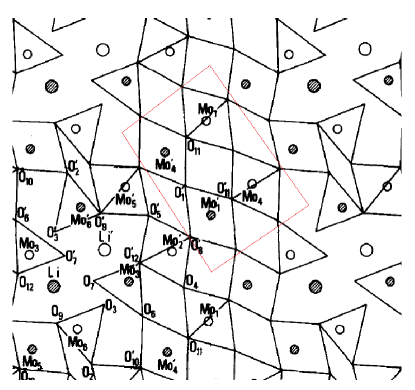
b)

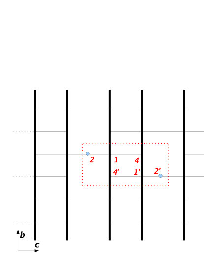
Figure 1: a) The crystal structure of purple bronze, after Ref.Onoda-structure-Xray . A cut perpendicular to highly conductive b-axis is shown. The atoms which belongs to zig-zag chains are indicated. b) A simplified structure of the low energy model. We show the top view on b-c plane. The $t$ and $t_{\perp}$ hoppings as given in the first line of hamiltonian Eq.2 are shown, sites 1 and 4 lie within the ladder, site 2 is outside it but $t_{\perp}$ hopping most likely goes through this site.

III Effective low energy hamiltonians

III.1 Tight-binding fermionic hamiltonian

The LDA-DFT results presented in Sec. II treat electron-electron interactions at the mean field level. It is assumed that a single electron moves in an average electrostatic potential. However it is known that the higher order terms in electron-electron interaction can bring very different physics, particularly in the case of reduced dimensionality. Thus we need to introduce them to our model.

The LDA results shows that a majority of carriers density at the Fermi energy is localized on zig-zag chains formed by the Mo(1) and Mo(4) octahedra (see Fig. 1a)). We can safely assume that the low energy physics is described by the dynamics of these electrons. Then the low energy hamiltonian formally writes:

$$H=-t^{b}_{1}\sum_{i\in even_{b},\sigma}c^{\dagger}_{i,\sigma}c_{i+\vec{b},\sigma}-t^{b}_{2}\sum_{i\in odd_{b},\sigma}c^{\dagger}_{i,\sigma}c_{i+\vec{b},\sigma}\\ -t^{c}_{1}\sum_{i\in even_{c},\sigma}c^{\dagger}_{i,\sigma}c_{i+\vec{c},\sigma}-t^{c}_{2}\sum_{i\in odd_{c},\sigma}c^{\dagger}_{i,\sigma}c_{i+\vec{c},\sigma}\\ -t^{a}\sum_{i,\sigma}c^{\dagger}_{i,\sigma}c_{i+\vec{a},\sigma}+h.c.+\\ \sum_{m,n,\sigma,\sigma^{\prime}}V_{nLDA}(r_{m}-r_{n})c^{\dagger}_{m,\sigma}c^{\dagger}_{n,\sigma^{\prime}}c_{n,\sigma^{\prime}}c_{m,\sigma}$$ (1)

where the vectors $\vec{b}=[0,b,0]$, $\vec{c}=[0,0,c]$, $\vec{a}=[a,0,0]$ define the $Li_{0.9}Mo_{6}O_{19}$ crystal lattice, summation runs over all ladder sites and depends on the parity of a given site index along directions $\vec{b}$ and $\vec{c}$. The $V_{nLDA}(r_{m}-r_{n})$ are the electron-electron interactions not included in the (mean-field) DFT calculation and the sum goes through positions of all carriers. The $t^{a-c}$ are hopping parameters along each crystal axis, as estimated in the previous section. As discussed there $t^{a}\approx 0$ (down to $0.1meV$) so we can neglect it for the ”high energy” range we are interested in. The electrons are moving exclusively within one slab (and mostly along the zig-zag chains). In Eq. 1 we kept only nearest neighbor hopping, since they are expected to be the dominant ones. The $t^{i}_{1,2}$ indicate a possibility of dimerization, namely different hoppings along i-th axis for even and odd bonds. Because Mo(1) and Mo(4) are crystallographically different we included the possibility that we are dealing with a dimerised chain, half-filled in the reduced Brillouin zone. We denoted the two corresponding hopping by $t^{b}_{1}$ and $t^{b}_{2}$. As explained in the previous section we take $t^{b}_{1}\approx t^{b}_{2}$ (with $10\%$ accuracy). The $t^{c}_{1,2}$ describe intra- and inter-ladder hopping respectively (see Appendix A). To lighten the notations we will denote from now on $t^{b}$ by $t$ and $t^{c}$ by $t_{\perp}$, to emphasize that they correspond respectively to hopping along and perpendicular to the chain direction.

The resulting simplified tight-binding model is shown on Fig. 1b). We simplify the interactions in a similar way, by explicitly considering the intra-chain and inter-chain parts of the interactions. The microscopic Hamiltonian we take is given by

$$H=-t\sum_{\langle i,j\rangle,\sigma}c^{\dagger}_{i,\sigma}c_{j,\sigma}-t_{1\perp}\sum_{\langle i,j_{1}\rangle,\sigma}c^{\dagger}_{i,\sigma}c_{j_{1},\sigma}-t_{2\perp}\sum_{\langle i,j_{2}\rangle,\sigma}c^{\dagger}_{i,\sigma}c_{j_{2},\sigma}\\ +U\sum_{i}n_{i\uparrow}n_{i\downarrow}+\sum_{m\neq n,\sigma,\sigma^{\prime}}V_{in}(r_{m}-r_{n})c^{\dagger}_{m,\sigma}c^{\dagger}_{n,\sigma^{\prime}}c_{n,\sigma^{\prime}}c_{m,\sigma}+\\ +\sum_{m\neq n,\sigma,\sigma^{\prime}}V_{out}(r_{m}-r_{n})c^{\dagger}_{m,\sigma}c^{\dagger}_{n,\sigma^{\prime}}c_{n,\sigma^{\prime}}c_{m,\sigma}$$ (2)

where $t=0.8eV$ (see Table.3) is hopping between nearest neighboring $i,j$ (denoted $\langle i,j\rangle$) molybdenum atoms along zig-zag chains (b-axis) and $t_{1,2\perp}$ are a hoppings in a perpendicular direction, within a slab (c-axis), between nearest-neighbors, $1$ is intra-ladder while $2$ is inter-ladder. The values of $t_{1,2\perp}$ are estimated in Appendix A and summarized in Tab.3. As already mentioned $t_{\perp}<20meV$, so we can treat it as a perturbation on the top of the intra-chain physics.

The strong correlations (last two lines in Eq.2) are usually parameterized by several quantities, which enter into the effective hamiltonian: $U$ is the local on-site interaction between charge densities of opposite spin $n_{i\uparrow}=c^{\dagger}_{i\uparrow}c_{i\uparrow}$ (Hubbard term), $V_{in}(r)$ is the interaction of two carriers placed inside the same chain at a distance $r\neq 0$, $V_{out}(r)$ is the interaction of two carriers placed in two different chains in a distance $r$ (both $V_{in}(r)$ and $V_{out}(r)$ are defined assuming an environment for which the LDA screening is included). We will discuss their strength in Sec. IV.1.

III.2 Bosonic field theory of a 1D system

In the following sections, it will be shown that the interchain couplings (both hopping and interactions) are reasonably weak compared to the intra-chain ones. We can thus anticipate the need to describe a strongly interacting one dimensional systems. In such a case, a very convenient formalism to incorporate the strong intra-chain interactions from the start is provided by the Luttinger liquid formalismgiamarchi_book_1d . This formalism allows to describe non-Fermi liquid state (Tomonaga-Luttinger liquid (TLL)) that occurs in one dimension as a result of the interactions.

The low energy dynamics of such a state is captured by collective, bosonic modes representing charge and spin density fluctuations. These fluctuations are connected to the two fields $\phi_{\nu}(x)$, where $\nu=\rho$ for charge fluctuations and $\nu=\sigma$ for spin fluctuations (linked with the fluctuations of charge and spin density). These fields have two canonically conjugate fields $\theta_{\nu}(x)$ linked with the respective currents fluctuations. In terms of these collective variables the hamiltonian readsgiamarchi_book_1d :

$$H_{0}=\sum_{\nu}\int\frac{dx}{2\pi}[(u_{\nu}K_{\nu})(\pi\Pi_{\nu})^{2}+(\frac{u_{\nu}}{K_{\nu}})(\partial_{x}\phi_{\nu})^{2}]$$ (3)

where $\Pi_{\nu}(x)=\frac{1}{\pi}\nabla\theta_{\nu}(x)$. All the intra-chain interactions conserving the momentum are now only fixing the precise values of the parameters $u_{\nu}$ (the velocities of the corresponding charge or spin density modes) or $K_{\nu}$ (the Luttinger parameters which control the decay of the various correlation functions).

In particular the local spectral function behaves as a power law $A(x=0,\omega,T=0)\sim\omega^{\alpha}$ with the following (interaction dependent) exponent:

$$\alpha=\frac{(K_{\sigma}+K_{\sigma}^{-1}+K_{\rho}+K_{\rho}^{-1})}{4}-1$$ (4)

For spin-rotationally invariant case $K_{\sigma}=1$, thus interactions, leading to the anomalous behavior, affects only the charge sector.

We can thus take (3) as our starting point for the chain physics, and study in the bosonized representation the effects of the various inter-chain coupling terms. This will ensure that at least the upper energy scales of the ”high energy” regime will be properly treated. The first step to determine the Luttinger parameters $u_{\nu}$ and $K_{\nu}$ is to estimate the strength of the various interactions, which we do in the following section (Sec.IV.1). At energies lower than the Fermi energy $E_{F}$ only two scattering channels are allowed $q\approx 0$ and $q\approx 2k_{F}$ (plus eventually higher harmonics). All density-density interactions, with small $q$ momentum exchange, can be incorporated into the hamiltonian given by Eq.3. They contribute to a highly non-trivial dependence of the TLL parameter $K_{\rho}$ (see Sec.IV.2).

The remaining interaction terms produce non-solvable hamiltonians of Sine-Gordon type, which in general is a functional $F[]$ of cosine terms:

$$H_{cos}=F[\cos(\sqrt{8}p\phi_{\nu}(x)),\cos(\sqrt{8}q\theta_{\nu}(x))]$$ (5)

where $p,q$ indicate higher harmonics (scattering with larger momenta exchange). Due to these terms the total problem allows only for approximate solution (at least in terms of continuous fields theory). The terms present in $H_{cos}$ are derived from large momentum exchange interactions (of both intra- and inter- chain origin). This is why their presence is analyzed carefully in the further sections. They are usually treated using Renormalization Group (RG) transformations, which allows to extract the terms that affect the most the TLL physics. This usually enables one to find the existence of gaps in the spectrum of bosonic modes, sometimes even to predict the ground state phase diagram. This kind of approach will be applied in Sec.VI.

IV Intra-chain physics

Let us first consider the physics taking place within a single chain. We want to obtain (in Sec.IV.1) the values of the various intra-chain interactions in (2) and from there (in Sec.IV.2) the values of the Luttinger parameters for the Hamiltonian (3).

IV.1 Strength of interactions

IV.1.1 U: local on-site interaction

A fully self-consistent calculation has been performed in Popovic-bron-DFT and a value $U=6.4$eV was found. This value seems at first sight surprisingly large (for $4d$ electrons), but a recent study using constrained-RPA Blugel-cRPA-U allows to understand this result. Although for bulk Mo $U\approx 3.8eV$, it was convincingly shown that the suppression of the pure Coulomb value $U_{0}\approx 14eV$ is mostly due to efficient screening in 3D of the d-electrons In our case (as discussed in details below) the system is underscreened, which entails also a significantly reduced plasmon frequency in comparison with the pure Mo (from $\sim 15eV$ to $0.65eV$ Blugel-cRPA-U ). Thus the value $U=6.4eV$ is justified or probably even modest. Then, if we take previously estimated hopping $t$, we get $U/t\approx 8$.

Note that this makes the local repulsion by far the largest energy scale in the problem.

IV.1.2 $V_{in}$: interaction inside a chain

In hamiltonian Eq.2 we defined intra-chain non-local interaction $V_{in}(r)$. In this subsection we will discuss its strength both in real and in momentum space $V_{in}(q)$. We are going to use shorthand notation $V_{in}\equiv V_{in}(r=b/2)$, as this is usually the single parameter which enters into so called $U-V$ model for a 1D chain. This parameter is much more difficult to estimate than $V_{out}$ (see Sec.V.1) as it involves the dynamics of the 1D metal. Rather than trying to estimate it directly from the interaction itself, we will simply adjust the value to be put in (2) and (3) in order to reproduce the experimental data on optical spectroscopy.

The ideaJacobsen-optic ; Mila-UV-optic is based on two independent estimates of kinetic energy in the system. The first one is related (by the optical sum rule) to the plasmon (edge) frequency $I_{p}=\omega_{p}^{2}$ and gives us the total possible kinetic energy available for the given number of carriers. The same quantity can be computed as an integral $I_{\sigma}$ of the optical conductivity $\sigma(\omega)$ (taken only over the highest conducting band). The point is that the second estimate gives us the real kinetic energy, renormalized by interactions.

Fortunately the necessary data is available for $Li_{0.9}MoO$. the value of of the plasmon frequency can be read out from Fig. 2 in Ref.Mandrus-optics and gives $\omega_{p}=0.65eV$ ($\omega_{p}$ extracted from the LDA Thomas is even larger $\approx 1.1eV$). The sum rule integral $I_{\sigma}$ was in fact already evaluated in Fig. 3 of Ref.Mandrus-optics . Determining the value of the first saturation from the plot has of course some error attached to it. We take $I_{\sigma}\approx 0.35$ ($\pm 5\%$). This value is reasonable because at higher energies one expects that the other bands start to intervene. The rest of the procedure is straightforward, the ratio of bare and interaction suppressed kinetic energy $I_{\sigma}/I_{p}$ equals to $\approx 0.83$. Then the results ofMila-UV-optic , together with the previously estimated value of $U$ allows to predict $V_{in}/t=1.2$ which means $V_{in}=0.95eV$ ($\pm>5\%$).

In addition to the interactions discussed up to now (which fit within the $U-V$ model for a single chain) there can also exist interactions between more distant neighbors (see Fig. 2). These interactions are non-zero because of the under-screening, a characteristic property of the 1D systems. When the separation is larger than that between nearest neighbor we can approximate the interaction by a continuum limit $V_{in}(r>b)=V_{\rm Coul}(r)/\epsilon(r)$ where $b=5.523\AA$ is a lattice constant along the b-axisOnoda-structure-Xray and $\epsilon(r)$ is a real space dielectric constant. In 2D and 3D systems the electrostatic potential is usually well screened thus the Thomas-Fermi approximation, already used in the DFT calculation, is sufficient. In our problem this means that for the very long length scales $r\gg a$ the potential is well screened, $V(r\gg a)=0$ (where $a=12.762\AA$ is the largest lattice constant, along the a-axis, perpendicular to the slabs planes), because then the network of the zig-zag chains can be thought as a homogenous 3D bulk. For shorter distances between the interacting electrons $r\approx a$ and then the distance between the neighboring chains does matter. The relation $a=2.1b$ implies that there are a few non-zero interaction terms $V_{in}(r)$ for $a\geq r>b$.

The screened potential inside 1D wire behaves approximately like $\ln(1/r)$ giamarchi_book_1d , same relation holds for the screening induced by the presence of other wires Alejandro-screen1D2D . In total we approximate that $V_{in}(q=0)$ will get renormalized by a factor $(1+\ln(a/b))\approx 1.6$. This gives a reasonable estimate for $V_{in}(q=0)$, however one has to be aware that for the value of charge mode TLL parameter the whole q structure has its importance.

The values of real and momentum space interactions are summarized in tables Tab.1 and Tab.2.

IV.2 Values of TLL parameter in the charge sector

Clearly the density-density interactions caused by $U$ and $V$ are not small perturbations compared to the kinetic energy. In fact they are the largest energy scale in the problem, larger than hopping along the chains. Thus they shall strongly affect the charge sector, they are strong enough to give rise to well pronounced non-Fermi liquid properties. We thus need to estimate the TLL parameters entering (3). As we will prove in later sections the following hierarchy of energies holds $U\gg V_{in}>t>V_{out}>J_{eff}$ (where $J_{eff}$ is an effective superexchange which determines energy scales for spin sector).

We thus start by solving the TLL problem for a single chain and will consider later the interchain couplings.

Even when $U\gg V_{in}>t$ we stay Haldane-1Dmain in a gapless phase within the TLL universality class, but computing the values of the Luttinger liquid parameters $K_{\rho}$ beyond the weak coupling limit is usually a very difficult problem giamarchi_book_1d , since one cannot compute them perturbatively.

In the present case we have to deal with a quarter filled system with a very small doping ($\delta$ around 2%), and a small dimerization (as we mentioned in Sec.III.1 it cannot be larger than 10% we take moderately 5% in any future calculations) and several non-zero interaction terms $V_{in}(r\geq b/2)$. As a first approximation we decided to analyze the physics of these zig-zag chains by looking at a quarter filled extended Hubbard chain with a local interaction $U$ and a nearest neighbor one $V$.

If $U$ is the larges energy scale in the problem then the charge sector can be mapped onto a spinless chain of fermions (or an XXZ spin chain) for which the exact TLL parameters are known Ejima-EPL-num ; giamarchi_book_1d . For a certain value $V_{in}$ we have

$$K_{\rho}^{XXZ}=\frac{\pi}{4\arccos\left[-\frac{V_{in}}{V_{in}^{c}(U)}\right]}$$ (6)

where $V_{in}^{c}(U)$ is the critical value of intra-chain nearest neighbor interaction for a given value $U$. When $U\to\infty$ the mapping is exact and the critical value is known $V_{in}^{c}(\infty)=2t$. In this case we get $K_{\rho}^{XXZ}=0.3$ which sets the lower limit for the TLL parameter. This is a rough estimate, but suggests that for further analysis we should use approaches which are valid for the gapless phase.

A more precise estimate can be obtained from a numerical study of the extended Hubbard model, and an estimation of the TLL parameters in the usual way via thermodynamic quantities Mila-Zotos-num ; Ejima-quart-dim-dop ; Ejima-EPL-num . From the relevant plots one reads out that our model is located somewhere in the range $K_{\rho}\in(0.3,0.37)$. One can try to give an even better estimate using Eq.6 even when U is not infinite (but still with U much larger that any other energy scale in the problem). It is commonly believed that the value $V_{in}^{c}(U)$ extracted from the numerics can give quite good approximation when substituted into (6). Estimates of critical $V_{in}^{c}(U)$ are usually done with higher precision, than for arbitrary $U,V$. In our case $U=8t$ implies $V_{in}^{c}(U)=2.6t$ Ejima-EPL-num ; Sano-num+RG and $V_{in}^{c}(U)=2.75t$ from older work by Mila and ZotosMila-Zotos-num . This gives $K_{\rho}=0.330$ (with $V/V_{c}=0.72$) or $K_{\rho}=0.340$. We have also followed the critical scaling analysis proposed in Sano-num+RG and found similar value $K_{\rho}=0.328$.

The exact solutions e.g. Bethe ansatz are available for a few special cases. If we include a (quite weak) dimerization and (very small) doping then the problem is located far away from any integrable model. However the influence of both these perturbations are known. The dimerization is able to lower a bit value of $K_{\rho}$, this effect can be present in particular in our case when we are not far from $V_{in}^{c}$ Ejima-quart-dim-dop . The doping has the opposite effect, however when one is not very close to critical point $K_{\rho}^{c}=1/4$ and close to commensurate case then the effect is negligible.

To conclude: the knowledge about the $U,~{}V_{in}$ we have collected above allowed us to give a several estimates based on complementary numerical calculations of $U-V$ models. All these estimates gives $K_{\rho}\in(0.3;0.36)$ (we allowed for 10% error in the $U,~{}V_{in}$ due to uncertainty of parameters). This is also in agreement with a very recent study for a system with finite range interactionAssaad-QMC : $K_{\rho}\approx 1/3$ when we take similar value of on-site term and account for the presence of $V_{in}(r)$ interactions up to four-five Mo sites. However in this last paper interactions with an exponential character were studied, which means that they decay much faster than those in our problem.

Note that this $K_{\rho}$ value is reasonably close to the one $K_{\rho}^{*}=1/4$ that would lead to a quarter-filled Mott insulator in the presence of an infinitesimal $V_{in}$. The system will be thus very susceptible to the precise value of $V_{in}$. Given the accuracy of our estimation we will take $K_{\rho}=1/3$ for further calculations. This value corresponds to the case for which the $4k_{F}$ charge fluctuations decay with the same exponent than the $2k_{F}$ charge and spin density fluctuationsgiamarchi_book_1d .

IV.3 The remaining interaction terms

By now we have studied interactions in real space (which we believe can be useful for numerical studies), while cosine terms beyond the TLL general expression (3) are defined in the reciprocal space representation. These values of scattering for large momenta exchange will be used as an input for the discussion done in Sec. VI.

The Hubbard $U$ interaction has a form of a delta function in real space thus in momentum space it contributes equally to small and large momenta exchange scattering (provided they are the intra-chain ones). The previous considerations also imply that, the Fourier transformed $V_{in}(q)$ is a weakly decaying function (slower than logarithm), so it affects the amplitude of scattering processes with large momenta exchange. As it was already expressed above the intrachain interactions are much larger then $t$ thus it is not straightforward to obtain the value of backscattering they cause. In fact the $K_{\rho}=1/3$ parameter given above, known from numerical studies of similar models, is a fixed point value $K_{\rho}^{*}$ which means that it contains a part of these contributions. Precisely it is the part included in the simplified $U-V$ model. The longer range, slower decaying interaction leads to smaller value of $K_{\rho}^{*}$. This suggests that the proper value of $K_{\rho}^{*}$ in our problem which contains long range interaction can be even smaller.

In our case the charge sector is renormalized by the possible umklapp terms $g_{3}$, so the last statement can be rephrased: the smaller final value of $K_{\rho}^{*}$ can be linked with larger value of initial, bare $g_{3}^{0}$. The precise estimation of the amplitude of $g_{3}^{0}$ is a very difficult task, the detail discussion of the bare large-q, intra-chain, term will be done in Sec. VI.

In addition, the $\epsilon(r)$ when computed using RPA (beyond standard DFT) gives a well known phenomena, the Friedel oscillations (in real space). The effect comes from the peculiar screening (singular susceptibility) at large momenta $q=2k_{F}$. In our case, due to the value of $k_{F}$ along chains, it gives an extra gain of energy for electrons located every second site. This affects the large momentum exchange part of interaction $V_{in}(q\sim 4k_{F})$. The value of this gain can be estimated using the fact that, for 3D metal, the additional oscillating part $V(r)\sim r^{-3}$ thus we give an estimation $V_{\rm Frid}\leq V_{in}(r=b)/8=0.1eV$. It is not as large as U or V, but can be significant if we compare it with $t_{\perp}$.

The U-V model that we have considered so far (in particular in Sec.IV.2) is of course only an approximation of the intra-chain physics and interactions. It should capture most of the effects at the energy scales we are considering, however it may slightly underestimate the strength of interactions.

IV.4 Spin mode

All the interactions considered up to now were connected with the charge sector. In 1D systems, because of the spin-charge separation, electrons spin degree of freedom should be discussed separately. For a half filled chain the knowledge about $t$ and $U$ allows to estimate the spin-spin exchange (superexchange) constant $J=t\frac{4t}{U}$. This determines the energies at which spin sector starts to play a role. The problem of purple bronze is more complex since the compound is quarter filled.

For such cases the formula for superexchange interaction can be still obtained from second order perturbation theoryEjima-quart-dim-dop . It reads:

$$J_{eff}=\frac{4t_{2}^{2}}{8t_{1}+2U+V_{in}-2\sqrt{(U-V_{in})^{2}+16t_{1}^{2}}}$$ (7)

where we have taken into a account the fact that due to dimerization there are two slightly different alternating hopping $t_{1}$ and $t_{2}$ along the chain taking $t_{2}-t_{1}\approx 0.05t$ and using the values of $U$ and $V_{in}$ obtained in Sec.IV.1 we obtain:

$$J_{eff}=0.2eV$$ (8)

It is indeed significantly smaller than $t$ (and also the charge sector interactions $U,V_{in}$) which implies that charge dynamics will dominate the $0.2-0.02eV$ energy range. However it is a non-negligible value in the sense that even for energies as high as $\omega\sim 0.1eV$ (in the middle of the considered ”high energy” regime) the spin excitations are coherent and dispersion is linear thus a TLL description with spin and charge modes is applicable. The spin-incoherent TLLFiete-RevModPhys-SILL is not an appropriate framework for our problem.

For a spin-rotational, SU(2) invariant model we have $K_{\sigma}(T=0)=1$. For the interacting case the spin velocity $u_{\sigma}$ is smaller than $v_{F}\approx 2t$, in particular $v_{\sigma}(U\rightarrow\infty)\rightarrow J$. This last value is comparable with the one observed in experimentJWAllen-1D+2D . The only candidate to break the SU(2) symmetry would be spin-orbit coupling $D_{LS}$ on the heaviest atom, molybdenum. A series of experimental and LDA studies allow to set its value in bulk bcc MoIverson-Mo-LS to $D_{LS}=100meV$. This value was obtained for the $\Delta$ point of a Brillouin zone in the Mo-bcc crystal. In our problem it should be smaller because the active electrons have mostly $t_{2g}$ character (with a larger $l$-number value). Thus $D_{LS}$ can be treated as a perturbation for $J$, contrary to $U$ for $t$ in a charge sector. This implies that $K_{\sigma}$ deviates from the non-interacting value $K_{\sigma}=1$ much less than $K_{\rho}$. To be precise from weak coupling theory (applicable in this case) we knowgiamarchi_book_1d :

$$K_{\sigma}=\sqrt{\frac{1+\frac{D_{LS}}{2\pi J}}{1-\frac{D_{LS}}{2\pi J}}}$$ (9)

from which we predict $K_{\sigma}=1.1$ which can increase the Green’s function exponent $\alpha$ only by $0.01$. The spin sector thus cannot be responsible for the experimentally observed values of the $\alpha$ exponent (defined in Eq.11) which are of order $\approx 0.5$. However the influence of the spin-orbit coupling should be taken into account when one studies the physics taking place lower energy scales, which are beyond the scope of this paper.

V Physics between the chains

After giving the description of a single chain physics we move beyond this model and study the strength (and the role) of interactions between carriers moving in different chains.

V.1 $V_{out}$: the values of interactions between the chains

The density-density interactions can be estimated as a standard Coulomb interaction between charges in a 3D dielectric, as it was done in Ref.Popovic-bron-DFT . Those authors gave estimate for a value of interaction from standard electrostatic Coulomb law (with the simplest static screening):

$$V_{out}(r=a)=\frac{1}{\kappa\epsilon_{0}a}$$ (10)

which in fact gives the value for two electrons in two different 2D slabs. We are more interested in interactions inside the slab which is obviously larger because (the smallest) interchain distance is then $c/2=0.4a$. A more fundamental problem is the value of the dielectric permittivity $\kappa$. In the previous work Popovic-bron-DFT the bulk $\bar{\kappa}\approx 10$ was used, which is typical for bulk semiconductors with similar value of a gap for oxygen states($\Delta_{O}\approx 2eV$). Taking into account the very weak metallic character along the c-axis the semiconductor approximation is correct. For further neighbors, with many oxygen atoms in between, one can take the bulk $\bar{\kappa}$ value. However for the nearest chains, as there is only one raw of oxygen atoms in the space between them, such large $\kappa$ value overestimates the screening provided by sparse environment. It is then convenient to take a function $\kappa(r)$ such that $\kappa(c/2)$ is reduced by $30\%$ in comparison with $\bar{\kappa}$. For larger $r$ distances at approximately $r\approx a$ it saturates to bulk value $\bar{\kappa}$. With this set of values we estimate $V_{out}=0.55eV$. For $r\rightarrow\infty$ the metallic character along b-axis intervene and $\kappa(r)\rightarrow\infty$. Thus the large distance interaction is strongly suppressed. In such a case the above estimated value for $V_{out}$ can be taken as the density-density interaction ($V_{out}(q\sim 0)$) between the nearest chains. The above estimate was done between two nearest chains which form a pair (see Fig. 2). On the other side of each chain there is another neighbor which is placed two times further. According to (10) these interactions $V_{out2}$ (we defined the inter-ladder term in analogy with e.g. $t_{c2}$ in Eq.33) are at least two times smaller. We then estimate (keeping $\kappa(r)$ in mind) $V_{out2}=0.2eV$.

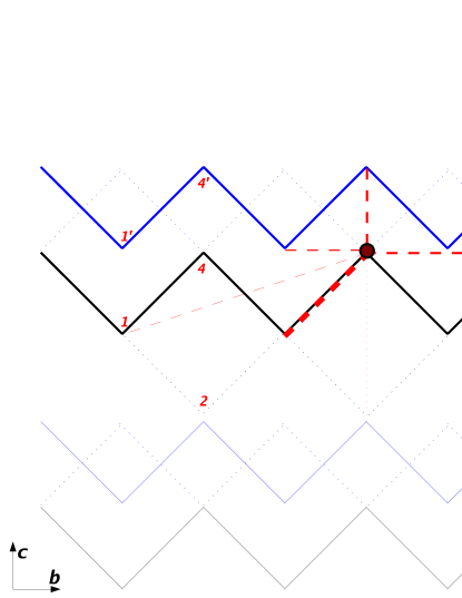
Figure 2: (color online) A real space image of strong interactions terms possible in purple bronze; the top view of a conducting slab is given. Interactions between an electron located on a dot-site and charges on different sites are indicated as red dashed lines of different thicknesses. Both $V_{in}$ (dashed lines within a black chain) and $V_{out}$ (dashed lines between the black and blue chains) are shown. The numbering of sites is like on Fig.1.

The treatment of terms with large momentum exchange is more complex. There is a $q=2k_{F}$ term which locks the interchain density wave, the so called $\pi-CDW$, which is shown on the Fig. 3a) . From the figure it is clear that the distances $r_{\pi}=\sqrt{(c/2)^{2}+(2k_{F})^{-2}}$ between charges in such configuration are rather large (around three times larger than the distance entering to previous calculation for $V_{out}(q=0)$) thus the screening is quite efficient and $\kappa[r_{\pi}]$ is definitely not reduced, but probably even enhanced with respect to the bulk value. In fact not only further chains, but also further slabs can intervene (because $r_{\pi}>a$).

There will be either a very efficient screening (like in a metal), or Coulomb potential approximation (but with enhanced $\kappa$) is still applicable. We assume, optimistically, the second case and use again (10). Two ways of proceeding are possible when one is interested in the staggered component of the interaction between two chains. In real space (direct application of (10)) one computes interactions with a linear set of dipoles. Due to increase of $\kappa(r)$ the interaction (with further dipoles) decays rapidly, which makes this straightforward approach quite tedious. In the reciprocal space approach one must take into account the fact that Fourier transform of $V_{out}(q)$ does decay in momentum space (it will be a $1/q$ decay in a 2D case corresponding to a separate slab). The second approach is simpler when one notice that the previously computed $V_{out}=0.55eV$ correspond to $q=0\pm(a/2)^{-1}$ (a distance between slabs sets the large distance cut-off). Then the $1/q$ scaling allows to estimate that $q=2k_{F}$ term will be suppressed by an extra factor four. Overall we have:

• a factor $1.5\div 2$ from the value $\kappa(r_{\pi})$

• a factor $1.5\div 3$ from the distance $r_{\pi}$

• a factor $\approx 4$ because we compute the staggered (large q) component

Taking all these factors into account we estimate that $2k_{F}$ component is reduced by at least one order of magnitude which means $V_{out}(q=2k_{F})<0.05eV$.

a)

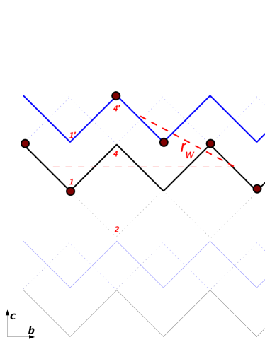
b)

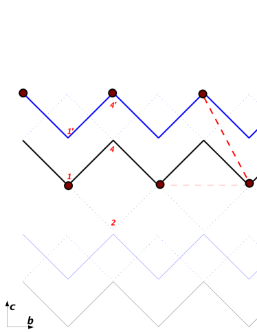
Figure 3: A schematic side view of a ladder structure (which enters to the low energy description of purple bronze) with: a) the $2k_{F}$ $\pi-$DW instability shown (The light, dashed line correspond to the distance $r_{\pi}$) b) the $4k_{F}$ $\pi-$DW instability shown.

There is also the $q=4k_{F}$ term. Now the distance is smaller, thus $\kappa$ is unaffected. However this term is strongly suppressed due to above mentioned Coulomb character of $V_{out}(q)$. At short distances corresponding to $r=(4k_{F})^{-1}$ the interaction may even have a 3D character (with no screening) thus $V_{out}\sim q^{2}$. By a similar reasoning like above we get $V_{out}(q=4k_{F})\approx 0.05eV$. The smallness of inter-chain large momenta terms (in comparison with density-density term) implies that the local field corrections are small, so our mean field model of screening is self-consistent. The influence of the inter-chain exchange interactions (both $2k_{F}$ and $4k_{F}$) on 1D physics will be discussed in Sec. VI.

To summarize the results for values of the strong coupling parameters found in the last two section we present all parameters in the tables Table 1 and Table 2.

Table 1: The real space values of strong coupling parameters (given in eV).

$U$	$V_{in}(r=b/2)$	$V_{in}(r=b)$	$V_{in}(r=2b)$	$V_{out}(r=c)$	$V_{out2}(r=2c)$
6.4	$0.95(\pm>5\%)$	0.5	0.2	0.55	0.2

Table 2: The reciprocal space values of strong coupling parameters (given in eV).

$V_{in}(q=0)$	$V_{in}(q=2k_{F})$	$V_{out}(q=0)$	$V_{out}(q=2k_{F})$	$V_{out}(q=4k_{F})$
1.6	see Sec.VI.2	0.55	$<0.05$	0.05

V.2 Luttinger liquid framework

The density-density interaction between the two neighboring chains $V_{out}(q=0)$ can be included on non-perturbative level. Because of the hierarchy of energies the presence of $V_{out}$ should be included on the top of 1D chain $K_{\rho}$. The zig-zag chains are grouped in pairs as shown on Fig. 1b) . Inside each pair we have two short links with interaction $V_{out}$ while in between them there is only one link with much smaller interaction $V_{out2}$. The ladder picture is then justified.

In the case of the ladder-like system (which means that there is either much stronger intra-ladder hopping $t_{1\perp}\gg t_{2\perp}$ or interaction) two more modes must be introduced. The problem can then be expressed in two different possible basis. One may work either in the chain basis with $\nu=\sigma 1,\sigma 2$ spin modes or in the total/transverse basis with symmetric and antisymmetric spin modes $\nu=\sigma S,\sigma A$ (and respectively the same for the charge sector). In general the Greens function $\alpha$ exponent can be expressed as:

$$\alpha=\frac{\sum_{\nu}^{N}(K_{\nu}+K_{\nu}^{-1})}{2N}-1$$ (11)

where $N$ is a number of modes. A significant $V_{out}(q=0)$ gives a preference for symmetric and antisymmetric modes as it can be diagonalized in this basis.

Thus within the ladder picture the two degenerate charge modes (in the two chains of the ladder) split into two holons with two different velocities. One of them (symmetric) describes the fluctuations of the total charge density, while the other one (anti-symmetric) describe the relative fluctuations in two different zig-zag chains. Their values are:

$$K_{\rho S,A}=\frac{K_{\rho}}{1\mp K_{\rho}V_{out}/(\pi v_{F})}$$ (12)

The respective values are: $K_{\rho S}\approx 0.30$ and $K_{\rho A}\approx 0.38$. For energies well below $V_{out}$ the hamiltonian of the charge sector is given as a sum of two bosonic modes plus a non-linear part $H_{\rm cos}$ caused by large-q (exchange) interactions:

$$H_{eff}=\sum_{\nu}\int\frac{dx}{2\pi}[(u_{\nu}K_{\nu})(\pi\Pi_{\nu})^{2}+(\frac{u_{\nu}}{K_{\nu}})(\partial_{x}\phi_{\nu})^{2}]\\ +H_{\rm cos}$$ (13)

where as explained in Sec.III.2 now the summation goes over four modes $\nu=\rho S,\rho A,\sigma S,\sigma A$. If we neglect $H_{\rm cos}$ then the single-hole propagator (relevant for ARPES), the density Greens function with chirality $\vartheta$:

$$G_{\vartheta}^{<}(x,t)=\langle\psi_{\vartheta,\sigma}^{{\dagger}}(x,t)\psi_{\vartheta,\sigma}(0,0)\rangle$$ (14)

is knownOrgad_A-LL and can be written as a simple generalization of the standard TLL result, as a product of four gapless modes. For example for the right going hole:

$$G_{R}^{<}(x,t)=\prod_{\nu}g_{\zeta_{\nu}}(x,t)$$ (15)

where:

$$g_{\zeta_{\nu}}=\left[(x-v_{\nu}t)\right]^{\zeta_{\nu}}\left[(x+v_{\nu}t)\right]^{\zeta_{\nu}}$$

with the exponents $\zeta_{\nu}=(K_{\nu}+K_{\nu}^{-1})/8$. For a numerical values of these exponents in our model and their implications see Sec.VII.1.

In the case when $H_{cos}$ is able to open a gap in a given mode, the respective term in the product in Eq.15 should be substituted by a modified Bessel function of a second kind, which gives the expected exponential decay of correlation function.

The inter-ladder interaction $V_{out2}$ are significantly smaller and thus will not bring any novel physics at higher energy scales (above 10meV), so this leave them out of the scope of this work.

VI Renormalization Group study

VI.1 Statement of the problem with the inter-chain operators

The interactions with small momentum exchange can be absorbed in a definition of TLL parameters, but obviously there are also scattering channels with the large momentum exchange. These generate cosine type terms, which in principle can bring us away from TLL universality class as defined in Eq.3. There are several terms which are expressed as cosine operators in the bosonization language. In addition to previously incorporated umklapp terms there are the ones which emerge from the inter-chain interactions. It is because usually they are the most pertinent for the ladder system. They are:

$q_{1}=2k_{F}$

these are interactions originating from the presence of $V_{out}(q=2k_{F})$; they have a form $\cos(2\phi_{\rho A})\cos(\sqrt{2}\phi_{\sigma 1})\cos(\sqrt{2}\phi_{\sigma 2})$

$q_{2}=4k_{F}$

these are interactions originating from the presence of $V_{out}(q=4k_{F})$; they have a form $g_{\perp}^{\pi}\cos(4\phi_{\rho A})$, and (only in the commensurate case) the inter-chain umklapp $g_{\perp}^{u}\cos(4\phi_{\rho S})$

$t_{\perp}$

the single particle hopping induce several cosine operators Khveshchenko-RGtperp , each of them in the form $\cos(2\theta_{\rho A})F[\cos(\sqrt{2}\phi_{\sigma 1}),\cos(\sqrt{2}\phi_{\sigma 2})]$, where functional $F[]$ is a linear combination (there are also higher order hopping terms, but as they are proportional to $t_{\perp}^{2}$ we can safely neglect them)

The standard way to treat these terms is deriving, perturbatively (usually on the single-loop level), the renormalization group (RG) equations giamarchi_book_1d . The RG equations allows us to predict weather a given term will increase and affect the low energy physics (become relevant) as the running energy variable $\Lambda\approx max[\omega,T]$ decreases. To be precise the quantity $l$ entering to RG equations is defined as $\Lambda\sim\exp(-l)$ or to be precise $l=\ln(\Lambda/W)$, where $W=2t$. This last formula allows to link two quantities (which we will do throughout this section), however one should remember that while $l$ is just a number, $\Lambda$ has an energy unit. In the following we apply the following convention $g_{\perp}^{\pi}[\Lambda_{1}]=V_{out}(q=4k_{F})/\bar{\Lambda}$ where $\bar{\Lambda}=\pi v_{F}$.

The naive way would be to add RG equations describing these terms into the previously determined TLL fixed point. Unfortunately, in our particular problem this approach is not justified. Our problem can be stated as follows: one to incorporate the above given operators into the intra-chain, umklapp RG flow, which was already accounted for.

We expect that the following physics takes place. Around $200meV$ a gappless TLL appears and later undergoes the renormalization flow. At this finite energy we know the values of interchain terms caused by $V_{\perp}(q=4k_{F})$ as they were estimated in the previous section, but $g_{3}$ cannot be taken to be equal to zero (it is not yet a fixed point as explained in Sec.VI.2). If we want to treat all instabilities with $4k_{F}$ periodicity on equal footing then we have to begin the flow with non-zero intra-chain $g_{3}$ and see how it will compete or conspire with inter-chain instabilities. Estimating the value of the initial $g_{3}$ which we need to substitute into RG equations is a highly non-trivial task, our proposition on how to tackle this problem is given in appendix C.

VI.2 The intra-chain, umklapp RG flow

In Sec.IV.2 we have given the values of intra-chain TLL parameter $K_{\rho}$ within U-V model approximation. The point is that these are already renormalized, the fixed point values $K_{\rho}^{*}$, and as such already contain influence of intra-chain umklapp scattering.

The fact that this operator is there and affects $K_{\rho}^{*}$ becomes clear from the following reasoning. As mentioned above, we are working with weakly dimerized chains close to half-filling. In the reduced Brillouin zone $k_{F}=0.487\pi/b$ according to DFT and $k_{F}=0.51\pi/b$ according to ARPES. This discrepancy can be understood. One should remember that the precise value of $k_{F}$ can vary as it depends on the relative value of chemical potential inside a chain (determined also by strong correlations) with respect to the local potential on the $Li$ ion (donor of electron). In any case one must admit that the doping is low enough, so in the ”high energy regime” the zig-zag chain is not able to recognize whether it is doped or not.

In addition an important remark has to be kept in mind: the above form of umklapp operator is appropriate for a quarter filled chain. This approach holds for weakly dimerized zig-zag chain, to be precise for the case when amplitude of umklapp interaction is larger than dimerization. From the analysis of the DFT band structure we know that $t_{1}-t_{2}<0.1eV$. After evaluating the strength $g_{3}$ we also check if this assumption was consistent.

In this case the umklapp terms (so called $g_{3}$), in the i-th chain, in the form $cos(\sqrt{8}\phi_{\rho i})$, has to be taken into consideration. The RG equation for this instability reads:

$$\frac{\partial g_{3}}{\partial l}=8g_{3}(1/4-K_{\rho})$$ (16)

The critical value of TLL parameter for this operator is $K_{\rho}^{c}=1/4$, so it seems to be irrelevant in our problem. However in the case of Berezinskii-Kosterlitz-Thouless flow, like the one described by eq.16 there exists a straight line on the $g_{3}-K_{\rho}$ plane, a separatrix between relevance and irrelevance regime (gapped and critical phase). Essentially this is because the compressibility of charge mode will also change:

$$\frac{\partial K_{\rho}}{\partial l}=-8g_{3}^{2}K_{\rho}^{2}J_{0}(\delta^{eff}(l))$$ (17)

and for large enough values of initial $g_{3}$, this equation cannot be neglected, the RG flow cannot be assumed to be vertical as we did before. Thus the amplitude of bare coupling $g_{3}$ can play a role. As we will see below, in our problem the amplitude $g_{3}$ does matter.

In the equation Eq.17 we kept the doping dependence which is encoded inside the Bessel function of the first kind $J_{0}(\delta(l))$. However below we assume that doping is essentially equal to zero and we work in a commensurate case. This assumption comes from the fact as we work in a constant chemical potential (the chain is embedded in a whole crystal and one knows the chemical potential of such a system from DFT solution) the effective doping will get renormalized $\sim-g_{3}^{2}J_{0}(\delta^{eff}(l))$ already at higher energies. Because of the same reason we neglect the renormalization of the charge modes’ velocity $\sim g_{3}^{2}K_{\rho}J_{2}(\delta^{eff}(l))$. From now on all we neglect all doping dependence and set $\delta^{eff}=0$ in the ”high energy regime”.

VI.3 The RG analysis of the $4k_{F}$ terms

If the inter-chain $4k_{F}$ terms are considered alone then we immediately see that they are less relevant than the $2k_{F}$ instabilities described in Sec.VI.4 (it is because $K_{\rho\nu}^{c}=1/2$). However there are several reasons why we think that the $4k_{F}$ will be more important and decided to investigate it first. The $4k_{F}$ depend only on charge modes, which can be particularly important for energies larger than or comparable with $J$. What is more, as we deduced before, $K_{\rho}<1/3$ and then it is the $4k_{F}$ CDW instabilities which are decaying slower. Finally there is an intra-chain umklapp term with the same periodicity and large, bare amplitude.

Section Sec.VI.2 gave us necessary understanding of the intra-chain RG flow, now we can proceed and introduce inter-chain terms. The $q_{2}=4k_{F}$ $\pi-wave$ scattering has the following RG equation:

$$\frac{\partial g_{\perp}^{\pi}}{\partial l}=2(1-2K_{\rho A})g_{\perp}^{\pi}-g_{3}g_{\perp}^{u}$$ (18)

and the inter-chain umklapp:

$$\frac{\partial g_{\perp}^{u}}{\partial l}=2(1-2K_{\rho S})g_{\perp}^{u}-g_{3}g_{\perp}^{\pi}$$ (19)

In the above equations we have already introduced the so called mixed terms caused by the presence of $g_{3}$ term (see below for an explanation). We need to take the inter-chain terms together with the standard umklapp $g_{3}$ to get a complete RG flow. These terms will also affect the flow TLL parameters, the $K_{\rho S,A}$, the symmetric/antisymmetric TLL parameters, which are defined in different basis that the intra-chain $K_{\rho 1,2}$ ones (used in Eq.16 and 17). The intra-chain umklapp scattering may be rewritten in this basis using the fact that the combination of two umklapps can be expressed in a rather simple form:

$$g_{3}[\cos(2\sqrt{8}\phi_{\rho 1})+\cos(2\sqrt{8}\phi_{\rho 2})]=\\ 2g_{3}\cos(4\phi_{\rho A})\cdot\cos(4\phi_{\rho S})$$ (20)

where we assumed that umklapp $g_{3}$ is identical in both chains 1 and 2. This can be justified by the crystal symmetry argument.

In the following we work with the perturbation described by Eq.20 in the symmetric/asymmetric basis. We need to re-write the RG equations for the combined intra-chain umklapp. Instead of Eq.16 and Eq.17 now we have:

$$\frac{\partial g_{3}}{\partial l}=g_{3}(2-4(K_{\rho S}+K_{\rho A}))+2g_{\perp}^{u}g_{\perp}^{\pi}$$ (21)

$$\frac{\partial K_{\rho S}}{\partial l}=-K_{\rho S}^{2}\left(8g_{3}^{2}+(g_{\perp}^{u})^{2}\right)$$ (22)

$$\frac{\partial K_{\rho A}}{\partial l}=-K_{\rho A}^{2}\left(8g_{3}^{2}+(g_{\perp}^{\pi})^{2}\right)$$ (23)

where (in the last two equations) we have distinguished the two RG flows of symmetric and antisymmetric $K_{\rho}$s (instead of single Eq.17) and already included their dependence on inter-chain interactions $V_{out}$. These equations should be taken together with Eq.18 and Eq.19 to obtain the full RG flow. Below we show in Fig.4 the result of a direct integration of this system of differential equations as well as a semi-quantitative analysis of RG flow between energy scales corresponding to $\Lambda_{1}=0.2eV$ (where TLL is likely to form) and $\Lambda_{2}=0.02eV$. These are the limits of interest for the ”high energy regime” study. The physical reason of this limit will be given below.

One can dispute whether a direct integration is valid when $g_{3}$ and $y_{\parallel}$ (see App.C for $y_{\parallel}$ definition) are of order O(1). Such large terms could in principle generate significant higher order operators along RG. However there are no higher order terms proportional to $g_{3}^{n}$ ($n\geq 2$). Then the higher orders mixed terms will be either irrelevant (because of large $p$ value in functional Eq.5) or of quite small amplitude. Qualitatively the full RG flow can be thought as superposition of two BKT flows, two hyperbolas on $g_{i}-K_{\nu}$ plane.

Let us first check what are the amplitudes different instabilities $g_{i}$ at $\Lambda_{2}$, in the first order approximation. If we neglect the flow of $K_{\nu}(l)$ then the solution of the equations Eq.18, 19 21 is an exponential function:

$$g_{\nu}[2t*\exp(-l)]=g_{\nu}[\Lambda_{1}]\exp\left(\eta_{\nu}^{*}(-l-\ln(\Lambda_{1}/2t))\right)$$ (24)

where $\eta_{\nu}$ is the dimension of the operator $g_{\nu}$, e.g. $\eta_{\perp}^{\pi^{*}}=2(1-2K_{\rho A}^{*})$ The crucial approximation we made in Eq.24 is that we assumed exactly vertical flows and took the fixed point values of $K_{\nu}^{*}$, which tends to overestimate the strength of all instabilities. As a result of Eq.24 we get: $g_{3}[\Lambda_{2}]\bar{\Lambda}\approx 0.1eV$, $g_{\perp}^{\pi}[\Lambda_{2}]\bar{\Lambda}\approx 0.075eV$, $g_{\perp}^{u}[\Lambda_{2}]\bar{\Lambda}\approx 0.08eV$. Note that because initially $K_{\rho S}[\Lambda_{1}]<K_{\rho A}[\Lambda_{1}]$, the inter-chain umklapp $g_{\perp}^{u}$ renormalizes more than the $\pi-$DW one $g_{\perp}^{\pi}$, however one has to remember that its bare amplitude is smaller due to doping effects. Already this simplified reasoning shows that the amplitude of the irrelevant term even at $\Lambda_{2}$ is still larger than amplitudes of the relevant terms. This is a peculiarity of our problem. The presence of a mixed terms will in fact enhance this property: because $g_{\perp}^{u}\approx g_{\perp}^{\pi}<g_{3}$ then one can interpret Eq.18 and Eq.19 as if $K_{\rho S,A}^{c}$ was shifted from $1/2$ downwards. On the other hand in Eq.21 we see that inter-chain instabilities push (weakly) the RG flow of $g_{3}$ towards its separatrix.

Now let us move to the analysis of the $K_{\rho S,A}$ RG flows. From Eq.22 and Eq.23 we immediately realize that intra and inter-chain terms support each other in lowering the values $K_{\rho S,A}$. Taking into account the initial (at $\Lambda_{1}$) hierarchy of energies we can be sure that the initial flow of $K_{\rho\nu}\sim g_{i}^{2}$ will be dominated by $g_{3}^{2}$ while the reasoning of the previous paragraph showed that around $\Lambda_{2}$ both terms are equally important. Initially the flow slows down because an irrelevant $g_{3}$ decreases, but later it can speed up again due to relevant inter-chain instabilities as seen on figure Fig.4 where the result of numerically solving of Eq.22and Eq.23 is shown. Estimating quantitatively $K_{\rho S,A}[\Lambda_{2}]$ can be achieved in two ways.

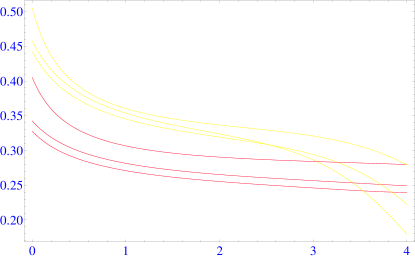
Figure 4: (color online) Three RG flows of $K_{\rho S}$ (red, three bottom curves at $l=0$) and $K_{\rho A}$ (yellow, three top curves at $l=0$) TLL parameters for different choices of initial parameters. The energy scale $\Lambda_{2}$ corresponds to $l\approx 3.5$. If all $K_{\nu}$ tend to be constant for increasing $l$, then the RG flow is so called ”vertical”. The initial values for three curves are (from top to bottom): (0.05, 0.04 , 0.5 , 0.5, 0.4);(0.05, 0.04 , 0.4 , 0.45, 0.35);(0.06, 0.05 , 0.38 , 0.45, 0.35); where the following notations are used $(g_{\perp}^{\pi}\bar{\Lambda},g_{\perp}^{u}\bar{\Lambda},g_{3}\bar{\Lambda},K_{\rho A},K_{\rho S})$. For the RG flow which give the bottom $K_{\rho S,A}$ curves, the instabilities (not shown) are large $g_{i}\approx 1$ at the scale $\Lambda_{2}$ which means that the RG flow should be stopped. The other two flows do not suffer from this limitation.

First way (i) assumes the independence of intra- and interchain BKT RG flows. We already know the influence of $g_{3}$ term alone, now we want to compute how much the $K_{\nu}[\Lambda_{2}]$ would be lowered during the BKT RG flow caused only by the inter-chain term, e.g. if we keep only $g_{\perp}^{\pi}$ term in Eq.23 for $K_{\rho A}[\Lambda_{2}]$. We can use the procedure very similar to the one applied in App.C, just that now we are moving towards $l\rightarrow\infty$ along the RG trajectory. By analogy with App.C reasoning we define the flow invariant $A_{\perp}$. In the case of this RG flow $g_{\perp}^{0}\approx 0.01\ll 1$ thus $A_{\perp}\approx(y^{\perp})_{\parallel}^{0}$, where $(y^{\perp})_{\parallel}^{0}=0.11$ is the distance of the bare $K_{\rho A}^{0}=0.39$ to $K_{\rho A}^{c}=1/2$. We then obtain (from an analog of Eq.47) that $y^{\perp}_{\parallel}[\Lambda_{2}]=0.15$, which means that RG flow caused $\Delta y^{\perp}_{\parallel}[\Lambda_{2}]=y^{\perp}_{\parallel}[\Lambda_{2}]-A_{\perp}\approx 0.05$ of the $K_{\rho A}[\Lambda_{2}]$ decrease . This additional change of $K_{\rho A}[\Lambda_{2}]$ should be added on the top of the value previously found from the U-V model (see Sec.IV.2) $K_{\rho A}^{*}\approx 1/3$. However, because of the $g_{3}$ influence, the $A_{\perp}$ is not a constant but it increases during the flow so the above value of the $\Delta y^{\perp}_{\parallel}[\Lambda_{2}]$ is underestimated. Such a deviation from a single BKT flow, particularly pertinent at lowest energies, is clear from figure Fig.5.

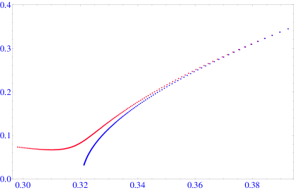
Figure 5: (color online) A comparison between BKT flow caused by a non-zero $g_{3}$ only (blue, bottom curve) and the result of our full RG flow (red, top curve). This is a parametric plot with $g_{3}[l]$ on the vertical axis and an average $(K_{\rho S}+K_{\rho A})/2$ on the horizontal axis. The initial values are: for blue line (0.0, 0.0 , 0.35 , 0.45, 0.35) and for red (0.06, 0.05 , 0.35 , 0.45, 0.35) with the same notation like in Fig.4.

The second way (ii) comes from the fact that, as pointed out above, the $g_{3}$ term dominates most of the RG flow between $\Lambda_{1}$ and $\Lambda_{2}$. Let us assume that the inter-chain terms effectively adds up to the initial amplitude of $g_{3}[\Lambda_{1}]$ (see Eq.20):

$$g_{3}^{eff}[\Lambda_{1}]\approx g_{3}[\Lambda_{1}]+A_{aux}*2*V_{out}(4k_{F})/\bar{\Lambda}$$ (25)

where the origin of $A_{aux}=0.6$ factor is explained in the end of this section. Taking into account the results of App.C we see that with this new effective amplitude of the umklapp the initial point of the RG is located quite close to the separatrix of intra-chain flow. The resulting value of $K_{\rho\nu}^{*}$ is then going to be close to $K_{\rho\nu}^{c}=1/4$. This obviously overestimates the change of $K_{\rho\nu}[\Lambda_{2}]$ because effectively in Eq.22 we took a square of a sum instead of a sum of squares. There is also a hidden assumption here that $K_{\rho A}\approx K_{\rho S}$, but looking at figure Fig.4 we see that this works well for all cases.

From the reasonings (i) (upper limit) and (ii) (lower limit) we conclude that within our approximation $K_{\rho S,A}\in(0.25,0.29)$. This is in agreement with the results presented on Fig.4 and Fig.5.

Finally we can try to estimate the value of a gap in the holon spectrum. We choose to work with $g_{\perp}^{\pi}$ as it has the strongest tendency to open a gap. We estimate the gap in the case if this instability was acting on its own when $\Delta\approx W\exp(-l^{*})$ where $g_{\perp}^{\pi}[W\exp(-l^{*})]=1$. For the specific cases the $l^{*}$ is knowngiamarchi_book_1d for example deep inside the gapped phase (self-consistent harmonic approximation) or close to the separatrix of RG. Unfortunately our problem does not belong to any of these, because $A_{\perp}\approx 0.12$ which for $\Lambda_{2}$ energy scale is neither very small nor very large. We approximate the flow of the considered $g_{\perp}^{\pi}$ by BKT flow which can be integrated out (see also App.C):

$$\arctan\left(\frac{y_{\parallel}^{0}}{A_{\perp}}\right)-\arctan\left(\frac{y_{\parallel}}{A_{\perp}}\right)=A_{\perp}l$$ (26)

If we use the fact that $y_{\parallel}^{0}\approx A_{\perp}$ and $y_{\parallel}[2t\exp(-l^{*})]\gg A_{\perp}$ (we are not far from the separatrix) then we get $A_{\perp}l^{*}\approx\pi/4$. In fact this value of $l^{*}$ is quite close to the ones we get from numerical integration of the full flow. Then the gap is:

$$\Delta_{\perp}^{\pi}=2t\exp\left[-\pi/(4A_{\perp})\right]$$ (27)

which gives $\approx 2meV$. The low initial value of the $V_{out}(q=4k_{F})$ translates into quite small expected value of the gap in the spectrum.

The lowest energy (below $\Lambda_{2}$) flow of umklapp processes are seriously affected by doping. If the $g_{\perp}^{\pi}$ is able to open a gap before that then these other RG equations will be changed by the presence of the gapped mode. For the intra-chain umklapp instability the initial point lies very close (esp. if we include terms beyond U-V model) to separatrix, which means that it is very susceptible to these modifications.

Usually in such a case one thinks about two competing instabilities taking place in two different basis (intra- and inter-chain). Our problem is different, the cooperation of instabilities is realized. This becomes clear if one assumes that he tends to be locked at minimum e.g. corresponding to $\sqrt{8}\phi_{\rho 1,2}=\pi$ (then $\cos(\sqrt{8}\phi_{\rho 1,2})=-1$). For this specific value of $\phi_{\rho 1,2}^{0}$ the combined inter-chain terms (see Eq.20) give non-zero and negative value ($A_{aux}\approx-0.6$). This corresponds to an additional energy gain caused by an auxiliary instability. It is a rare case when the two gaps does not exclude but can help each other. In particular this validates the assumption made in Eq.25.

VI.4 The analysis of the $2k_{F}$ terms

The RG equation for the $2k_{F}$ backscattering operator readsgiamarchi_book_1d :

$$\frac{\partial g_{\pi}^{2k_{F}}}{\partial l}=(2-K_{\rho A}-K_{\sigma A})g_{\pi}^{2k_{F}}$$ (28)

It is the most relevant instability (already for $K_{\rho A}<1$) if one assumes SU(2) symmetric case in the spin sector when $K_{\sigma A}=1$, so naively we would expect it to dominate the low energy physics. However there are details that matter. First, the initial amplitude of this term is quite low. Second, the RG flow of this term will be strongly perturbed:

• at high energies ($\Lambda\approx 0.2eV$) the spin sector is still in the incoherent regime, certainly the dispersion is not yet linear (mind the value of $J_{eff}$). Thus all terms which contain spin dynamics, like $\cos(\phi_{\sigma})$ will strongly fluctuate

• the $2k_{F}$ terms has to compete with $4k_{F}$ instabilities described in the previous section: large $g_{3}$ (in the initial part of the flow) and relevant $g_{\perp}^{\pi}$ and $g_{\perp}^{u}$ in the lower energies

• at lower energies ($\approx 0.015eV$) several terms generated by the perpendicular hopping ($\sim t_{\perp}$) will start to intervene. Although they are irrelevant (connected with the field $\theta_{\rho A}$ Khveshchenko-RGtperp ), still their initial amplitude is significantly (three times) larger than $V_{out}(q=2k_{F})$. We then expect that physics will be dominated by a competition between these two types of cosine terms, as it was studied in Ref.Suzumura-t-perpRG2 ; Suzumura-t-perpRG where the term confinement-deconfinement transition was coined to describe the physics.

Based on results from Ref.Suzumura-t-perpRG2 ; Suzumura-t-perpRG , one may expect that due to last mechanism the $2k_{F}$ instability is weakened. In any case because $K_{\rho A}\ll K_{\rho A}^{c}=1$ the $2k_{F}-$RG flow is vertical. This implies that $K_{\rho A}$ value (and thus also Green’s function $\alpha$ exponent) is very weakly affected by the presence of the $2k_{F}$ terms.

VII Discussion

VII.1 Comparison with experiment

In this last part we wish to compare the estimated Luttinger liquid parameters with experimental findings. Experiments look at low energy ($l>1$), long distance behavior ($r>k_{F}^{-1}$), which we should keep in mind for the rest of this section. The crucial question is: what is the value of TLL parameters $K_{\nu}$ that enters into measured correlation functions? Obviously the answer cannot depend on the point where we arbitrarily decide to stop the RG flow, one has to keep in mind that $g_{i}$ terms usually are still finite at such a point. As discussed in Ref.Schulz-corr-fun , the correlation functions are of the form:

$$R(r)=\left(\frac{r}{W}\right)^{K^{c}}\exp\left(\int_{0}^{r/W}y_{\parallel}[l]dl\right)$$ (29)

where $|r|=\sqrt{x^{2}+(v_{\nu}\tau)^{2}}$ is a distance in a time-space domain, W is an ultraviolet cut-off of the problem ($\sim 2t$), $y_{\parallel}[l]=K_{\rho}-K_{\rho}^{c}$ is a deviation of TLL parameter from the critical value $K_{\rho}^{c}$ of the considered flow. Thus the observed value could be interpreted not as $K[l]$, but rather as weighted average of $K[l]$ over longer and longer length-scales. In particular if we flow to a gapless phase then the observed $K_{\nu}$ corresponds to $K_{\nu}^{*}$, which is then equal to the invariant of the flow $A$.

Our problem is particularly difficult, because the answer to the above question strongly depends on yet unknown lowest energy physics. Indeed in our reasoning we have neglected several effects ($t_{\perp}$, $D_{LS}(q=2k_{F})$, proximity to Mott insulator, disorder) whose amplitudes are certainly smaller than $\Lambda_{2}\approx 20meV$ and which seriously harm TLL below this energy scale. Based on this we can reassure the validity of our approach only down to $\sim 20meV$.

Basically there are two distinct behavior which can occur at these lowest energy scales. First, one of the above mentioned perturbations can become pertinent just below the $\Lambda_{2}$ energy scale and thus stop the RG flow. In fact all these perturbation in one way or another would not support further lowering of $K_{\rho}$ value, thus the further $K_{\rho}[l]$ can be then taken as vertical. The observed TLL parameter should then be close to $K_{\rho}[\Lambda_{2}]$. The second possibility, which is not unlikely, is that 1D RG will remain valid down to much lower energies $\sim 1meV$ (see Sec.VII.2). Then as indicated in Fig.5 the RG trajectory always stays close to separatrix. This statement is in fact quantified by the values of invariants of the intra- and inter-chain RG flows: $A_{3}\approx A_{\perp}$, so it is always either $g_{3}[l]$ or $g_{\perp}[l]$ keeping us close to separatrix. Then Eq.29 gives a power low with a $K_{rho}^{c}=1/4$ exponent times a logarithmic corrections in the form $\log(r/W)$.

We are able to compare our results only with the experimental data corresponding to the ‘high energy’ range $\Lambda\in(0.02;0.2)eV$. In fact this is also the energy scale down to which, with no experimental doubt, the TLL persist. One should also keep in mind that the TLL $\alpha$ exponent should be computed within the ladder model introduced in Sec.V.2. In the following we assume that it is only $K_{\rho}$ responsible for $\alpha\neq 0$, while $K_{\sigma}=1$. Several different techniques have been used to measure the $\alpha$ exponent. These include PES and ARPES (4-150meV; 5-300K), STM(0-50meV; 10-50K), resistivity(30-300K); where in parenthesis we have indicated temperature and frequency ranges where the fits were performed. We see that at least one of them is always larger than $\Lambda_{2}$ which makes our theory applicable. All probes are consistent and gave the spectral function exponent $\alpha\approx 0.55\div 0.6$ which means $\bar{K}_{\rho}\approx 0.24\div 0.25$. This is reasonably close to $K_{\rho S,A}[\Lambda_{2}]\in(0.25,0.29)$ predicted theoretically in Sec.VI.3, but also to $K_{\rho}^{c}=1/4$. This shows the importance of the proximity to the Mott transition: it can cause a strong renormalization of $K_{\rho}$ TLL parameters towards lower values and thus observed large value of $\alpha$ exponent.

One can be even more explicit: the only way to obtain values $\alpha>1/2$ (which translates into $K_{\rho}<0.27$) in our model is by assuming that the combined $4k_{F}$ perturbations (intra-chain $g_{3}$ together with $g_{\perp}^{\pi}$ and $g_{\perp}^{u}$ terms) can drive the RG flow and lead to strong renormalization of the charge TLL parameters. There is one more argument which supports this scenario. It is lack of spinon peak which has not been observed in any PES (or ARPES) experiment in the last two decades. This can be justified theoretically only if $\alpha>1/2$, which provides strong limitations for the expected $\bar{K}_{\rho}^{*}$ values.

There is one experimental result which requires a comment. It is the temperature dependence of $\alpha$ invoked in Ref.JWAllen-alphaRG , based on ARPES results. There the following value $\alpha=0.9$ was measured at high temperatures. This means $(K_{\rho S}+K_{\rho A})/2+(K_{\rho S}^{-1}+K_{\rho A}^{-1})/2\approx 6$ which translates into $\bar{K}_{\rho}^{*}\approx 0.17$. This value is much smaller than our predictions. We would like to emphasize that within TLL theory such behavior is very unlikely. To be precise: as explained above it is not allowed to say that these different values comes out different points along RG trajectory. One model can possibly have only one ground state described by $\bar{K}_{\rho}^{*}$. In our opinion the observed temperature dependence can originate from a significant influence which phonons occupancy have on the LDA band broadeningThomas The fact that $\alpha(T)$ dependence seems to change with sample preparation (see Fig. 3d in JWAllen-alphaRG ) strongly supports this interpretation. Then the real value of $\alpha$ is the low energy one.

The other result is the estimate of a gap which according to our reasoning may be potentially opened by the $4k_{F}$ instabilities. However the value has been found to be extremely small $\sim 1meV$, thus our procedure, which relies on the RG analysis starting from 200meV, is insufficient to make any definite claims. What is more this value is much smaller than $\Lambda_{2}$, while there are several effects (like disorder or the interchain hopping $t_{\perp}$) which are potentially of order $\Lambda_{2}$ and destructive for such a gap. If the hierarchy of amplitudes was opposite (gap much larger than $t_{\perp}$) then the gap would suppress single particle hopping. In our case the outcome is unclear. Certainly a more sophisticated theory is necessary to understand the unusual physics taking place below 20meV. Experimentally this is also a controversial issue. Such a gap (in the charge sector or in $A_{TLL}(\omega)$) has never been seen in any experiment probing $\omega>3meV$. So far the only exception are low temperature resistivity measurementsHussey-rhoB , but even there a clear Arhenius-type activation behavior (at around 1meV) is preceded by an unusual power law like behavior.

VII.2 The validity of 1D approximation

It is knowngiamarchi_book_1d that the strong correlation effects (the formation of Luttinger liquid) are able to strongly reduce the value of $t_{\perp}$. To be more precise they strongly reduce the energy scale where system gains coherence along c-axis. With the value of the $\alpha$ exponent discussed above the perpendicular hopping $t_{\perp}$, will get strongly renormalized down to an effective value:

$$t_{\perp}^{eff}=t\left(\frac{t_{\perp}}{t}\right)^{\left(\frac{1}{2-\zeta}\right)}$$ (30)

where $\zeta=\alpha+1$ is a single particle Greens function exponent, and $\eta_{t\perp}=2-\zeta$ is a scaling dimension of the hopping operator. This gives a suppression of $t_{\perp}$ by a factor $\approx 20$. To be precise this means that due to the presence of strong interactions the hopping in the perpendicular direction becomes coherent only $\approx 1meV$.

On the top of it there is also another source of $t_{\perp}$ renormalization, which originates from the competition with the terms $V_{out}(q=2k_{F})$ (as described in Sec.VI.4). The $2k_{F}$ terms which are a functional of a charge asymmetric mode $\phi_{\rho A}$(e.g. the one inducing a $\pi-$DW) tend to suppress $t_{\perp}$ Suzumura-t-perpRG . Their influence is non-zero only when spin sector becomes coherent and $t_{\perp}$ is sufficiently small (there is a Bessel function $J_{0}(t_{\perp}[l])$ involved, which arises in a very similar way like the one in Eq.17). It was shown Suzumura-t-perpRG2 ; Suzumura-t-perpRG that the significant suppression of $t_{\perp}$ may happen only when $t_{\perp}[l]\approx V_{out}(q=2k_{F})$, which (according to scaling given in Eq.30) can be the case in our problem but only for energies below $\Lambda_{2}$.

The frustration of the nearest and the next-nearest perpendicular hopping also suppress the coherence of perpendicular hopping also on second order when e.g. particle-hole processes are considered. This is immediately visible if one writes a formula for any susceptibility $\chi(q,q_{\perp},\omega)$ within the mean field, RPA level:

$$\chi(q,q_{\perp},\omega)=\frac{\chi^{TLL}(q,\omega)}{1+(2t_{\perp}\cos(q_{\perp}c/2)+2t^{\prime}_{\perp}\cos(q_{\perp}c))\chi^{TLL}(q,\omega)}$$ (31)

where we are using simplified version of perpendicular dispersion $\varepsilon(\vec{q_{\perp}})$ known from Eq.33. We see that the sign difference between $t_{\perp}$ and $t^{\prime}_{\perp}$ can cause a suppression of a second term in the denominator. This obviously weakens the $q_{\perp}$ dependence of susceptibility (thus also a corresponding observable), but also has its influence if one wished to develop a perturbative series to study the influence of $t_{\perp}$.

Finally there are also disorder effects which can localize carriers in the perpendicular direction. They are described in the next section.

From experiments (optical spectroscopy, Kadowaki-Woods ratio) we know that 1D physics seems to be correct even down to 2meV. In the light of the above discussion these statements are not unreasonable. Thus, the assumption about validity of 1D physics should be valid even down to few meV’s and certainly in the ”high energy” range of energies (200-20meV) this paper is dedicated for. The values of TLL parameters indeed strongly support the idea that the 1D regime should be able to persist to temperatures much lower than the bare perpendicular hopping.

VIII How pertinent is substitutional disorder?

The most likely source of a disorder in purple bronze are random vacancies of $Li$ atoms. From the DFT resultsThomas we know that energy shifts caused in this way within dispersive bands can be at most 15meV (when the $Li$ are completely removed). This sets the strength of the substitutional disorder potential. Because $Li$ atoms are placed well outside zig-zag chains it is reasonable to assume the Coulomb potential interaction ($\sim q^{2}$) between impurity and TLL, with predominant small q-exchange scattering. Thus the disorder will have primarily forward character and $D_{f}\approx 15meV$.

Thus we can assume the model of TLL with a forward disorder to check if it explains the observed temperature anomalies of ARPES below 200K. The spectral function for forward disorder is known in real space:

$$A(x,t)=A_{TLL}(x,t)\exp\left(-\frac{D_{f}K_{\rho}^{2}}{u_{\rho}^{2}}x\right)$$ (32)

where $A_{TLL}$ is the pure Luttinger liquid spectral function, which is known e.g. see Eq.15. The behavior of the Fourier transform is easy to extract in the limits of large and small $\omega$. For the high-energy (15-150meV) range we expect the $A_{TLL}$ power law scaling (because we work above the energy range disorder can affect). This is definitely not seen in experimental data JWAllen-Tscal . For the low energies (2-15meV) we expect a convolution of standard TLL signal with an exponential decay. A broadening of $A_{TLL}$ was indeed observed, but it was suggestedAllen-latest that the Gaussian convoluted with the LL $A_{TLL}(q,\omega)$ provides better fit of the ARPES data. If one looks back how the eq.32 was derived she/he finds that the approximation of uncorrelated scattering events is not obeyed. The presence of a Gaussian is like if the scattering events were not random, but momentum conserving. There is also discrepancy on the level of energy scales, experimentally the broadening has been observed already at 20meV which is larger than the maximal amplitude of disorder 15meV.

Let us now move to discussion of the lowest temperatures effects. By analogy with a reasoning in Sec.V.1 we expect that $D_{f}$ is accompanied with a component which provides source of random scattering events with large momentum exchange. Its amplitude should be one order of magnitude smaller and thus could potentially affect only the lowest energy scales. Taking into account the $\alpha$ exponent value (and repulsive character of interactions $K_{\rho}\ll 1$) the backward disorder, if present, has to be highly relevant. It is known that in 1D systems the backward disorder, in the form of cosine operator, when present kills the superconductivity (of the BCS type). Experimentally the unusual ARPES was observed precisely for the superconducting samples. As expected for more disordered samples the superconductivity disappeared, while the broadening of ARPES signal around 100K was unchanged. The disorder also does not fit well neither with magnetoresistivity nor STM experiments. It is also claimed (from optical spectroscopy) that the mass of remaining mobile carriers decreases below 30K.

In conclusion this simplest notion of disorder is incompatible with observed effects. However the discussion is not yet closed. The strength of the disorder potential $D_{f}$ is comparable with the zero point motion or the thermal expansion effects, which will certainly affect its influence. The crystal structure is quite complex and supports much more sophisticated mechanisms e.g. the relative rotations of different $Mo$ octahedra. These rotations provide another source of disorder in the material. However from the overall analysis of the structure it is certain that all these microscopic effects should affect $t_{\perp}$ stronger than the inside-chain Luttinger liquid physics. What is more $t_{\perp}\approx D_{f}$ which means that relative strength of disorder is quite large.

IX Conclusion

We studied the low energy physics of a quasi-1D material, lithium molybdenum purple bronze. Already before it has been shown that this material is extremely anisotropic, there is a linear dispersion along b-axis extending down to 0.4eV, while in the perpendicular direction dispersion is at least two orders of magnitude weaker. In this study the physics is expressed in terms of field theory. Our work cover the energy range where the physics of charge modes, holons describes well the dynamics of the compound. It begins at around 0.2eV where the experiment has clearly shown an emergence of 1D spectral properties, in particular the fermionic bands seem to merge at this energy scale giving rise to a single entity. The regime of our interest extends as low as 1D physics is strictly valid. To be on the safe side we set it at around 20meV which is larger than any of the possible disturbances.

The starting point of our study is the recent LDA-DFT result where the peculiar band structure of the material has been re-confirmed. Based on this we construct the effective low energy theory: the band structure around Fermi energy is casted into a tight-binding model. In addition a minimal model has to contain the strong correlation terms, laying beyond LDA-DFT approximation. The aim of the next few section is to provide the quantitative description of these strong interactions.

We begin with parameterizing the interactions taking place inside a single zig-zag chain. From previous experimental and numerical works we are able to extract an effective real space model with a physically reasonable values of strong correlation parameters. Due to sparse arrangement of the chains the interactions have a finite range character, however in the first approximation we use U-V model to obtain the values of Luttinger liquid parameter $K_{\rho}$. This estimate is based on several numerical works dedicated for models which are very similar to ours. All values converge at $K_{\rho}\approx 1/3$, which is rather low value, in particular it may allow $4k_{F}$ instabilities to dominate the physics. It also suggests that the umklapp processes are at play. In addition we also investigate the effects which can arise if one goes beyond simplistic U-V model. A separate section is dedicated to a spin sector, where we estimate basic energy scales.

Later parts of this work are devoted to inter-chain physics. As the chains are grouped in a well distinguishable pairs, it is tempting to propose a description within a ladder-like model. We use dielectric approximation in order to estimate strength of inter-chain interactions, considering processes with both small and large momenta exchange. With this knowledge we propose that the description of physics in the considered charge regime should be done within framework of Luttinger liquid consisting of four modes, the two charge modes corresponds to the total (symmetric) and the transverse (asymmetric) fluctuations. This description fully incorporates the inter-chain processes with small momentum exchange together with the intra-chain physics.

The processes with large momentum exchange can be taken as perturbation and treated within RG approach. However, we claim that in order to achieve a valid description of the system one has to consider the intra-chain umklapp together with them. We derive a full system of RG equations which cover intra- as well as inter-chain instabilities and study possible trajectory of the flow. This allows us to develop a description of purple bronze down to the limits of validity of 1D theory. In the discussion we show that these limits can be safely extended to energy scales two or even three times smaller than 20meV. This allowed us to make a more extensive, quantitative comparison with experimental results, which basically confirms our theoretical insight into this complicated compound.

We have achieved the effective low energy description of $Li_{0.9}Mo_{6}O_{17}$ compound which is able to explain convincingly experimental findings down to 20meV. In particular we showed that for the specific combination of parameters, which are present in this material, an unusual situation may occur. Due to their mutual competition, the critical phase (the Luttinger liquid) is able to survive down to the very low energy scales. Despite the two leg ladder formation, no gap opens in holons spectra (at least not above 20meV). This is contrary to the usual case where a significant gap is present in a transverse (asymmetric) mode of a ladder-like low-dimensional system. Such an unusual physics is in agreement with the physics extracted from experimental investigations.

It is likely that for the lowest energies the purple bronze falls into category of doped Mott insulators with extremely small gap, but further developments of the theory are necessary to make any definite claims about this highly interesting regime.

Appendix A Derivation of tight-binding parameters

The central result of DFT calculation is a band structure of a given material. As it contains a huge amount of information usually it is difficult to deal with when the effective, low energy theory is constructed. In such a case a standard procedure is to approximate a solid by a tight binding model with a selected sites located at their positions $r_{i}$ and unknown hopping parameters between them. Usually only the nearest $t$ and the next-nearest $t^{\prime}$ neighbor hoppings are taken into account. We are interested in the low energy physics, thus the aim is to fit bands crossing Fermi energy $E_{F}$ (in the given direction $d$) with the properly chosen parameters $t_{d}$ $t^{\prime}_{d}$.

As described in Sec.II in the case of $Li_{0.9}Mo_{6}O_{17}$ most of low energy spectral weight in located on $Mo(1)$ and $Mo(4)$ sites (see Fig.1a)) so we take only them into further considerations. As explained only two bands cross $E_{F}$ thus our aim is to fit these two dispersions.

The dispersion relation for tight-binding model defined above is known:

$$\varepsilon(\vec{k})=-t\cos(k_{b}b/2)-t^{\prime}\cos(k_{b}b)\\ -\frac{t_{\perp 1}+t_{\perp 2}}{2}\cos(k_{c}c/2)-\frac{t_{\perp 1}-t_{\perp 2}}{2}\sin(k_{c}c/2)\\ -\frac{t^{\prime}_{\perp 1}+t^{\prime}_{\perp 2}}{2}\cos(k_{c}c)-\frac{t^{\prime}_{\perp 1}-t^{\prime}_{\perp 2}}{2}\sin(k_{c}c)$$ (33)

where the first line describes the dispersion along b-axis, the last two the dispersion along c-axis (with the dimerization included). We neglected dispersion along a-axis. For the b-axis dispersion we assumed the simplest tight-binding model, as the LDA result suggest rather straightforward interpretation of the bands. We introduced next nearest neighbor hopping $t^{\prime}$ mostly because the zig-zag chain structure seems to allow for this refinement, however from the general shape of bands in $\vec{b}$ direction it does not seem to be necessary.

For the c-axis dispersion the situation is quite different. We introduced much more terms because the curve is quite unusual, with a well pronounced double minima and a node at $k_{c}=0$, a feature quite difficult to fit within standard model. Based on the analysis of the structure presented in Fig.1a) we deduce that:

i

there are two times more intra-ladder than inter-ladder links (they are linked either directly through $Mo(1)-Mo(4)$ bond or auxiliaries through $Mo(2)-Mo(5)$ bond)

ii

the inter-ladder hopping goes always though $Mo(2)$ (or $Mo(5)$) atoms, these are two paths which can interfere. These hoppings are possible only every second site.

iii

the next-nearest neighbor hopping is allowed only through $Mo(2)-Mo(5)$ thus should be much smaller than the one above. These hoppings are also possible only every second site.

all of the hoppings goes either via a $\delta$-bonds or $\pi$-bonds (the second are allowed only due to octahedra tilting). None of the links should be very much stronger than the others. From the crystal structure analysis all other hopping should be negligible, thus the task is to fit the dispersion with the above given model Eq.33.

On Fig.6 we show an example of $k_{c}$ dispersion with conditions [i]-[iii] fulfilled. We see that it is possible to obtain quite similar shape to the LDA one provided that two interfering paths have the hopping parameters of the opposite sign. The only quantitative issue would be relatively large value of band splitting found in Ref.Thomas . It may appear from Hartree interaction term if the two bands had different orbital character. One should also remember that the value of splitting found in Popovic-bron-DFT was a bit smaller. We will leave this issue for further specialized studies like e.g. NMTO.

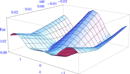
Figure 6: The dispersion along c-axis shown for varying direct $\delta$ hopping along $Mo(1)-Mo(4)$ bond. The strength of the other hopping path (through $Mo(2)-Mo(5)$) is taken as 0.02 while the inter-ladder one 0.01.

These findings are summarized in a table Tab.3

Table 3: The values of parameters (given in meV) of the tight binding hamiltonian given in Eq.33 which fits best the LDA resultThomas , the dispersion along c-axis.

$t_{\perp 1}$	$t_{\perp 2}$	$t^{\prime}_{\perp 1}$	$t^{\prime}_{\perp 2}$
15	5	-10	$<5$

Appendix B Derivations of cosine terms

We begin with a fermionic for of considered scattering processes: 1. the intra-chain umklapp:

$$H_{cos3}^{i}=g_{3}\sum_{q_{i}}(\psi_{+q_{1}i\uparrow}^{{\dagger}}\psi_{+q_{2}i\downarrow}^{{\dagger}}\psi_{-q_{3}i\downarrow}\psi_{-q_{4}i\uparrow}+\\ \psi_{-q_{1}i\uparrow}^{{\dagger}}\psi_{-q_{2}i\downarrow}^{{\dagger}}\psi_{+q_{3}i\downarrow}\psi_{+q_{4}i\uparrow})$$ (34)

2. Interchain umklapp scattering ($4k_{F}$):

$$H_{cos3}^{\perp}=g_{3}^{\perp}\sum_{q_{i}}(\psi_{+q_{1}1\uparrow}^{{\dagger}}\psi_{+q_{2}2\downarrow}^{{\dagger}}\psi_{-q_{3}2\downarrow}\psi_{-q_{4}1\uparrow}+\\ \psi_{-q_{1}1\uparrow}^{{\dagger}}\psi_{-q_{2}2\downarrow}^{{\dagger}}\psi_{+q_{3}2\downarrow}\psi_{+q_{4}1\uparrow})$$ (35)

where the following relation between momenta holds $q_{1}+q_{1}-q_{1}-q_{1}=0$ in order to preserve momentum conservation during scattering; the low energy limit implies that for each momenta there exist the ultraviolet cut-off $|q_{i}|<\Lambda$.

3. Interchain exchange scattering ($4k_{F}$):

$$H_{cos}^{\pi}=g_{\pi}^{4k_{F}}\int_{0}^{L}dx\rho_{1}^{4k_{F}}\rho_{2}^{4k_{F}}$$ (36)

4. Interchain exchange scattering ($2k_{F}$):

$$H_{cos}^{\pi}=g_{\pi}^{2k_{F}}\int_{0}^{L}dx\rho_{1}^{2k_{F}}\rho_{2}^{2k_{F}}$$ (37)

where $\rho_{i}^{2k_{F}}$ is the $2k_{F}$ charge density in the i-th chain.

Usually one is also interested in correlation functions, which have the general form:

$$R_{O}=<T_{\tau}O(x,t)O^{{\dagger}}(0,0)>$$ (38)

where the simplest intra-chain examples of possible operators $O$ are:

• in Peierls channel - the charge density wave (CDW)
  $O_{CDW}(x,t)=\sum_{r,\sigma,\sigma^{\prime}}\psi_{r}(x,t)^{{\dagger}}\delta_{\sigma\sigma^{\prime}}\psi{\bar{r}}(x,t)$

• in Cooper channel - the singles superconductivity (SS)
  $O_{SS}(x,t)=\sum_{r,\sigma,\sigma^{\prime}}\sigma\psi_{r}(x,t)\delta_{\sigma\bar{\sigma^{\prime}}}\psi_{\bar{r}}(x,t)$

When we consider a single chain then a chiral fermion creation operator is related to bosonic spin and charge fields as follows (in the continuum limit):

$$\psi_{r,\sigma}(x)=\frac{1}{\sqrt{2\pi\alpha}}\eta_{r,\sigma}\exp(\imath rk_{F}x)\exp-\imath/\sqrt{2}(r\phi_{\rho}(x)-\theta_{\rho}(x)+\sigma(r\phi_{\sigma}(x)-\theta_{\sigma}(x)))$$ (39)

where the coefficient $\eta_{r,\sigma}$ is the Majorana fermion which doesn’t have any spatial dependance and it is introduced only in order to preserve anti-commutation for the fermion operators $\psi$. Usually they don’t play any role in the physical description of the system but they are able to change signs of some correlation functions, so one has to take care about them.

In the case of the ladder one has a straightforward generalization:

$$\psi_{r,\sigma,\nu}(x,t)\sim\eta_{\sigma,\nu}\exp(\imath rk_{F}x)\exp[-\frac{\imath}{2}(r\phi_{+\rho}+\theta_{+\rho}+\sigma(r\phi_{+\sigma}+\theta_{+\sigma})+\nu(r\phi_{-\rho}+\theta_{-\rho}+\sigma(r\phi_{-\sigma}+\theta_{-\sigma})))]$$ (40)

The above given equations Eq.39 and Eq.40 allow to rewrite all fermionic terms in the hamiltonian like e.g. the one in Eq.34 or in general any interesting operator into the language of bosonic fields. In our particular case we are interested in the following interaction terms:

1. Umklapp scattering (at quarter filling) in the i-th chain

$$H_{cos3}=g_{3}\int_{0}^{L}dx\cos(2\sqrt{8}\phi_{i\rho}(x)+\delta)$$ (41)

where $\delta$ indicates the doping away from a commensurate case, quarter filling in our case (where $\exp\imath(\pi-4k_{F})x$ is not oscillating).

2. Interchain umklapp scattering ($4k_{F}$):

$$H_{cos3}^{\perp}=g_{3}^{\perp}\int_{0}^{L}dx\cos(4\phi_{S\rho}(x)+\delta)$$ (42)

3. Interchain exchange scattering ($4k_{F}$):

$$H_{cos}^{\pi}=g_{\pi}^{4k_{F}}\int_{0}^{L}dx\cos(4\phi_{A\rho}(x))$$ (43)

4. Interchain exchange scattering ($2k_{F}$):

$$H_{cos}^{\pi}=g_{\pi}^{2k_{F}}\int_{0}^{L}dx\cos(2\phi_{A\rho}(x))\cos(\sqrt{2}\phi_{1\sigma}(x))\cos(\sqrt{2}\phi_{2\sigma}(x))$$ (44)

These are the terms for which RG equations are derived in Sec.VI. In all the above we took a following convention:

$$\phi_{S,A}(x)=\frac{\phi_{1}(x)\pm\phi_{2}(x)}{\sqrt{2}}$$ (45)

which allows to go from one basis to another.

Appendix C Initial value of umklapp terms

Estimating the value of $g_{3}$ at certain energy scale $\Lambda_{0}$ is an impossible task, so all our results cannot be taken strictly quantitatively. This is a generic problem of the RG method present for any model even a simple half filled chain. The complexity of our system, makes the task even more tedious.

We propose the approach, based on the first order expansion of RG equations, to get a reasonable value of $g_{3}(\Lambda_{0})$. However one has to keep in mind that as we are are working with rather large couplings, of order 0.1 (but always smaller than 0.25) so higher order terms can introduce non-negligible corrections even within single instability flow. Thus the results has to be taken with caution, can be thought as only approximation.

With this remarks being said we can proceed. One can in principle integrate out BKT equations to get a values of along the flow. One gets the following resultgiamarchi_book_1d :

$$g[l]=\frac{A}{\sinh\left[Al+\tanh^{-1}(A/y_{\parallel}^{0})\right]}$$ (46)

$$y_{\parallel}[l]=\frac{A}{\tanh\left[Al+\tanh^{-1}(A/y_{\parallel}^{0})\right]}$$ (47)

where A is an invariant of the flow, in our case $A=1/12$. Every point on an RG trajectory leads us to fixed point value $K_{rho}^{*}$. From numerics based on U-V model we found (Sec.IV.2) $K_{rho}^{*}=1/3$ and we know that for quarter-filled chain $K_{rho}^{c}=1/4$. Thus in our case $A=K_{rho}^{*}-K_{rho}^{c}=1/12$. Our aim is to extract the value of $K_{rho}[l]=K_{rho}^{c}+y_{\parallel}[l]$ at certain energy scale $\Lambda_{1}$ (corresponding to $\approx 0.2eV$) which upon RG leads to known $K_{rho}^{*}$. This procedure can be thought as moving against the direction of the RG flow.

The only missing quantity in Eq.47 is $y_{\parallel}[l=0]$ which should be interpreted as the distance of an initial point of the flow $K_{rho}[l=0]$ (formally in the infinite energy, i.e. somewhere around UV-cut-off of the model) from $K_{rho}^{c}=1/4$. Although around the fixed point the flow is rather vertical, we decided to take the most conservative (and giving the most modest value of $g_{3}(\Lambda_{0})$) assumption that $K_{rho}[l=0]=1/2\Rightarrow y_{\parallel}[l=0]=1/4$. It is because certainly at $K_{rho}=1/2$ the quarter filled chain remains insensitive to Mott localization.

With this we are able to estimate the bare $g_{3}(\Lambda_{1})\bar{\Lambda}$ to be around $0.35eV$. Then $y_{\parallel}(\Lambda_{1})$ is only 6% larger than corresponding $g(\Lambda_{1})$, while the position of the separatrix of RG flow in the first order is set by $y_{\parallel}=g$. The distance from the separatrix is of the same order like additional intra-chain terms described in Sec.IV.3. From the remarks above we know this is only an estimate, but it certainly implies that the umklapp, even in intra-chain U-V approximation, is an order of magnitude larger than any of $V_{\perp}(q=4k_{F})$. Although it seems to be irrelevant, but its bare amplitude is large and quite close to separatrix so the intra-chain umklapp has to be taken with care in the RG analysis below.

The fact that bare $g_{3}^{0}$ falls very close to separatrix can be confirmed by an independent reasoning. The position of separatrix is frequently constrained by symmetry considerations. Taking into account the hierarchy of energy scales, we take simplistic approximation of spinless fermions in $U\rightarrow\infty$ (like in Sec.IV.2). This obviously overestimates $g_{3}$, but numerics Mila-Zotos-num shows us that beyond a threshold $U=4t$, the dependence on U is weak, thus the corrections breaking (particle-hole) symmetry should be quite small. The advantage is that now one can map charge sector on pseudo-spin model (empty and occupied sites), for which the position of separatrix of RG flow (phase transition) in terms of bare parameters is known exactly thanks to SU(2) symmetry. It is located at $V_{in}^{eff^{c}}=2t^{eff}$ where $V_{in}^{eff}$ accounts for all unscreened interactions along the chain (while $t^{eff}\approx t$, if one want to be more precise he would found it slightly reduced with respect to $t$ because of dimerization). If we put values found before (in table Tab.2 for $V_{in}^{eff}$) we indeed find ourself very close to $V_{in}^{eff^{c}}$.

References

- (1) W.H. McCarroll and M. Greenblatt. Preparation of lithium molybdenum oxide bronzes by a temperature gradient flux growth technique. Journal of Solid State Chemistry, 54(2):282 – 290, 1984.
- (2) J. D. Denlinger, G.-H. Gweon, J. W. Allen, C. G. Olson, J. Marcus, C. Schlenker, and L.-S. Hsu. Non-fermi-liquid single particle line shape of the quasi-one-dimensional non-cdw metal : Comparison to the luttinger liquid. Phys. Rev. Lett., 82:2540–2543, Mar 1999.
- (3) J. Hager, R. Matzdorf, J. He, R. Jin, D. Mandrus, M. A. Cazalilla, and E. W. Plummer. Non-fermi-liquid behavior in quasi-one-dimensional . Phys. Rev. Lett., 95:186402, Oct 2005.
- (4) M. Greenblatt, W.H. McCarroll, R. Neifeld, M. Croft, and J.V. Waszczak. Quasi two-dimensional electronic properties of the lithium molybdenum bronze, li0.9mo6o17. Solid State Communications, 51(9):671 – 674, 1984.
- (5) Xiaofeng Xu, A. F. Bangura, J. G. Analytis, J. D. Fletcher, M. M. J. French, N. Shannon, J. He, S. Zhang, D. Mandrus, R. Jin, and N. E. Hussey. Directional field-induced metallization of quasi-one-dimensional . Phys. Rev. Lett., 102:206602, May 2009.
- (6) Nicholas Wakeham, Alimamy F. Bangura, Xiaofeng Xu, Jean-Francois Mercure, Martha Greenblatt, and Nigel E. Hussey. Gross violation of the wiedemann-franz law in a quasi-one-dimensional conductor. Nat. Commun., 2:396, 2011.
- (7) J. Choi, J. L. Musfeldt, J. He, R. Jin, J. R. Thompson, D. Mandrus, X. N. Lin, V. A. Bondarenko, and J. W. Brill. Probing localization effects in purple bronze: An optical-properties investigation. Phys. Rev. B, 69:085120, Feb 2004.
- (8) J. L. Cohn, B. D. White, C. A. M. dos Santos, and J. J. Neumeier. Giant nernst effect and bipolarity in the quasi-one-dimensional metal . Phys. Rev. Lett., 108:056604, Feb 2012.
- (9) J. Chakhalian, Z. Salman, J. Brewer, A. Froese, J. He, D. Mandrus, and R. Jin. Magnetism in purple bronze. Physica B: Condensed Matter, 359(0):1333 – 1335, 2005.
- (10) M. Onoda, K. Toriumi, Y. Matsuda, and M. Sato. Crystal structure of lithium molybdenum purple bronze li0.9mo6o17. Journal of Solid State Chemistry, 66(1):163 – 170, 1987.
- (11) C. A. M. dos Santos, B. D. White, Yi-Kuo Yu, J. J. Neumeier, and J. A. Souza. Dimensional crossover in the purple bronze . Phys. Rev. Lett., 98:266405, Jun 2007.
- (12) M. S. da Luz, J. J. Neumeier, C. A. M. dos Santos, B. D. White, H. J. Izario Filho, J. B. Leão, and Q. Huang. Neutron diffraction study of quasi-one-dimensional lithium purple bronze: Possible mechanism for dimensional crossover. Phys. Rev. B, 84:014108, Jul 2011.
- (13) G.-H. Gweon, J. W. Allen, and J. D. Denlinger. Generalized spectral signatures of electron fractionalization in quasi-one- and two-dimensional molybdenum bronzes and superconducting cuprates. Phys. Rev. B, 68:195117, Nov 2003.
- (14) G.-H. Gweon, J. D. Denlinger, J. W. Allen, C. G. Olson, H. Höchst, J. Marcus, and C. Schlenker. Non-fermi liquid angle resolved photoemission line shapes of . Phys. Rev. Lett., 85:3985–3985, Oct 2000.
- (15) Feng Wang, S.-K. Mo, J. W. Allen, H.-D. Kim, J. He, R. Jin, D. Mandrus, A. Sekiyama, M. Tsunekawa, and S. Suga. Case for bulk nature of spectroscopic luttinger liquid signatures observed in angle-resolved photoemission spectra of . Phys. Rev. B, 74:113107, Sep 2006.
- (16) G.-H. Gweon, S.-K. Mo, J. W. Allen, J. He, R. Jin, D. Mandrus, and H. Höchst. Luttinger liquid angle-resolved photoemission line shapes from samples of grown by the temperature-gradient-flux technique. Phys. Rev. B, 70:153103, Oct 2004.
- (17) Piotr Chudzinski, Thomas Jarlborg, and Thierry Giamarchi. cond-mat/arxiv:1203.1827.
- (18) Z. S. Popović and S. Satpathy. Density-functional study of the luttinger liquid behavior of the lithium molybdenum purple bronze . Phys. Rev. B, 74:045117, Jul 2006.
- (19) Myung Hwan. Whangbo and Enric. Canadell. Band electronic structure of the lithium molybdenum purple bronze li0.9mo6o17. Journal of the American Chemical Society, 110(2):358–363, 1988.
- (20) Feng Wang, J. V. Alvarez, S.-K. Mo, J. W. Allen, G.-H. Gweon, J. He, R. Jin, D. Mandrus, and H. Höchst. New luttinger-liquid physics from photoemission on . Phys. Rev. Lett., 96:196403, May 2006.
- (21) C. A. M. dos Santos, M. S. da Luz, Yi-Kuo Yu, J. J. Neumeier, J. Moreno, and B. D. White. Electrical transport in single-crystalline : A two-band luttinger liquid exhibiting bose metal behavior. Phys. Rev. B, 77:193106, May 2008.
- (22) T. Giamarchi. Quantum Physics in One Dimension. Oxford University Press, Oxford, 2004.
- (23) Ersoy Şaşıoğlu, Christoph Friedrich, and Stefan Blügel. Effective coulomb interaction in transition metals from constrained random-phase approximation. Phys. Rev. B, 83:121101, Mar 2011.
- (24) C S Jacobsen. Trends in the infrared and near infrared properties of organic conductors. Journal of Physics C: Solid State Physics, 19(28):5643, 1986.
- (25) Frédéric Mila. Deducing correlation parameters from optical conductivity in the bechgaard salts. Phys. Rev. B, 52:4788–4793, Aug 1995.
- (26) Alejandro M. Lobos and Thierry Giamarchi. Dissipative phase fluctuations in superconducting wires capacitively coupled to diffusive metals. Phys. Rev. B, 82:104517, Sep 2010.
- (27) F. D. M. Haldane. Effective harmonic-fluid approach to low-energy properties of one-dimensional quantum fluids. Phys. Rev. Lett., 47:1840–1843, Dec 1981.
- (28) S. Ejima, F. Gebhard, and S. Nishimoto. Tomonaga-luttinger parameters for doped mott insulators. EPL (Europhysics Letters), 70(4):492, 2005.
- (29) F. Mila and X. Zotos. Phase diagram of the one-dimensional extended hubbard model at quarter-filling. EPL (Europhysics Letters), 24(2):133, 1993.
- (30) Satoshi Ejima, Florian Gebhard, and Satoshi Nishimoto. Tomonaga-luttinger parameters and spin excitations in the dimerized extended hubbard model. Phys. Rev. B, 74:245110, 2006.
- (31) K. Sano and Y. Ōno. Critical behavior near the metal-insulator transition in the one-dimensional extended hubbard model at quarter filling. Phys. Rev. B, 70:155102, Oct 2004.
- (32) Martin Hohenadler, Stefan Wessel, Maria Daghofer, and Fakher F. Assaad. cond-mat/arxiv:1201.3626.
- (33) Gregory A. Fiete. Colloquium: The spin-incoherent luttinger liquid. Rev. Mod. Phys., 79:801–820, Jul 2007.
- (34) R. J. Iverson and L. Hodges. Molybdenum: Band structure, fermi surface, and spin-orbit interaction. Phys. Rev. B, 8:1429–1432, Aug 1973.
- (35) Dror Orgad. Spectral functions for the tomonaga-luttinger and luther-emery liquids. Philosophical Magazine Part B, 81(4):377–398, 2001.
- (36) D. V. Khveshchenko and T. M. Rice. Spin-gap fixed points in the double-chain problem. Phys. Rev. B, 50:252–257, Jul 1994.
- (37) M. Tsuchiizu, P. Donohue, Y. Suzumura, and T. Giamarchi. Commensurate-incommensurate transition in two-coupled chains of nearly half-filled electrons. Eur. Phys. J. B, 19(2):185–193, 2001.
- (38) M. Tsuchiizu and Y. Suzumura. Confinement-deconfinement transition in two coupled chains with umklapp scattering. Phys. Rev. B, 59:12326–12337, May 1999.
- (39) T. Giamarchi and H. J. Schulz. Correlation functions of one-dimensional quantum systems. Phys. Rev. B, 39:4620–4629, Mar 1989.
- (40) Feng Wang, J. V. Alvarez, J. W. Allen, S.-K. Mo, J. He, R. Jin, D. Mandrus, and H. Höchst. Quantum critical scaling in the single-particle spectrum of a novel anisotropic metal. Phys. Rev. Lett., 103:136401, Sep 2009.
- (41) J. W. Allen, Lenart Dudy, Feng Wang, J. He, A. Sekiyama, and S. Suga. unpublished.
- (42) Krishnaji Parmendu Kant and Ramji Srivastava. Dielectric permittivity and breakdown strength of molybdenum trioxide films. Journal of the Physical Society of Japan, 39(5):1316–1318, 1975.